Matrix-Free Convex Optimization Modeling

Abstract

We introduce a convex optimization modeling framework that transforms a convex optimization problem expressed in a form natural and convenient for the user into an equivalent cone program in a way that preserves fast linear transforms in the original problem. By representing linear functions in the transformation process not as matrices, but as graphs that encode composition of linear operators, we arrive at a matrix-free cone program, i.e., one whose data matrix is represented by a linear operator and its adjoint. This cone program can then be solved by a matrix-free cone solver. By combining the matrix-free modeling framework and cone solver, we obtain a general method for efficiently solving convex optimization problems involving fast linear transforms.

1 Introduction

Convex optimization modeling systems like YALMIP [Lof04], CVX [GB14], CVXPY [DB], and Convex.jl [UMZ⁺14] provide an automated framework for converting a convex optimization problem expressed in a natural human-readable form into the standard form required by a solver, calling the solver, and transforming the solution back to the human-readable form. This allows users to form and solve convex optimization problems quickly and efficiently. These systems easily handle problems with a few thousand variables, as well as much larger problems (say, with hundreds of thousands of variables) with enough sparsity structure, which generic solvers can exploit.

The overhead of the problem transformation, and the additional variables and constraints introduced in the transformation process, result in longer solve times than can be obtained with a custom algorithm tailored specifically for the particular problem. Perhaps surprisingly, the additional solve time (compared to a custom solver) for a modeling system coupled to a generic solver is often not as much as one might imagine, at least for modest sized problems. In many cases the convenience of easily expressing the problem makes up for the increased solve time using a convex optimization modeling system.

Many convex optimization problems in applications like signal and image processing, or medical imaging, involve hundreds of thousands or many millions of variables, and so are well out of the range that current modeling systems can handle. There are two reasons for this. First, the standard form problem that would be created is too large to store on a single machine, and second, even if it could be stored, standard interior-point solvers would be too slow to solve it. Yet many of these problems are readily solved on a single machine by custom solvers, which exploit fast linear transforms in the problems. The key to these custom solvers is to directly use the fast transforms, never forming the associated matrix. For this reason these algorithms are sometimes referred to as matrix-free solvers.

The literature on matrix-free solvers in signal and image processing is extensive; see, e.g., [BT09a, BT09b, CEN06, CP11, GO09, ZPB07]. There has been particular interest in matrix-free solvers for LASSO and basis pursuit denoising problems [BT09b, CDS98, FGZ12, FNW07, KKL⁺07, vdBF09]. Matrix-free solvers have also been developed for specialized control problems [VB93, VB95]. The most general matrix-free solvers target semidefinite programs [KS09] or quadratic programs and related problems [SKM⁺13, Gon12b]. The software closest to a convex optimization modeling system for matrix-free problems is TFOCS, which allows users to specify many types of convex problems and solve them using a variety of matrix-free first-order methods [BCG11].

To better understand the advantages of matrix-free solvers, consider the nonnegative deconvolution problem

$$\begin{array}[]{ll}\mbox{minimize}&\|c*x-b\|^{2}\\ \mbox{subject to}&x\geq 0,\end{array}$$ (1)

where $x\in{\mbox{\bf R}}^{n}$ is the optimization variable, $c\in{\mbox{\bf R}}^{n}$ and $b\in{\mbox{\bf R}}^{2n-1}$ are problem data, and $*$ denotes convolution. Note that the problem data has size $O(n)$. There are many custom matrix-free methods for efficiently solving this problem, with $O(n)$ memory and a few hundred iterations, each of which costs $O(n\log n)$ floating point operations (flops). It is entirely practical to solve instances of this problem of size $n=10^{7}$ on a single computer [KB77, LLS04].

Existing convex optimization modeling systems fall far short of the efficiency of matrix-free solvers on problem (1). These modeling systems target a standard form in which a problem’s linear structure is represented as a sparse matrix. As a result, linear functions must be converted into explicit matrix multiplication. In particular, the operation of convolving by $c$ will be represented as multiplication by a $(2n-1)\times n$ Toeplitz matrix $C$. A modeling system will thus transform problem (1) into the problem

$$\begin{array}[]{ll}\mbox{minimize}&\|Cx-b\|^{2}\\ \mbox{subject to}&x\geq 0,\end{array}$$ (2)

as part of the conversion into standard form.

Once the transformation from (1) to (2) has taken place, there is no hope of solving the problem efficiently. The explicit matrix representation of $C$ requires $O(n^{2})$ memory. A typical interior-point method for solving the transformed problem will take a few tens of iterations, each requiring $O(n^{3})$ flops. For this reason existing convex optimization modeling systems will struggle to solve instances of problem (1) with $n=10^{4}$, and when they are able to solve the problem, they will be dramatically slower than custom matrix-free methods.

The key to matrix-free methods is to exploit fast algorithms for evaluating a linear function and its adjoint. We call an implementation of a linear function that allows us to evaluate the function and its adjoint a forward-adjoint oracle (FAO). In this paper we describe a new algorithm for converting convex optimization problems into standard form while preserving fast linear functions. (A preliminary version of this paper appeared in [DB15].) This yields a convex optimization modeling system that can take advantage of fast linear transforms, and can be used to solve large problems such as those arising in image and signal processing and other areas, with millions of variables. This allows users to rapidly prototype and implement new convex optimization based methods for large-scale problems. As with current modeling systems, the goal is not to attain (or beat) the performance of a custom solver tuned for the specific problem; rather it is to make the specification of the problem straightforward, while increasing solve times only moderately.

The outline of our paper is as follows. In §2 we give many examples of useful FAOs. In §3 we explain how to compose FAOs so that we can efficiently evaluate the composition and its adjoint. In §4 we describe cone programs, the standard intermediate-form representation of a convex problem, and solvers for cone programs. In §5 we describe our algorithm for converting convex optimization problems into equivalent cone programs while preserving fast linear transforms. In §6 we report numerical results for the nonnegative deconvolution problem (1) and a special type of linear program, for our implementation of the abstract ideas in the paper, using versions of the existing cone solvers SCS [OCPB15] and POGS [FB15] modified to be matrix-free. (The details of these modifications will be described elsewhere.) Even with our simple, far from optimized matrix-free cone solver, we demonstrate scaling to problems far larger than those that can be solved by generic methods (based on sparse matrices), with acceptable performance loss compared to specialized custom algorithms tuned to the problems.

We reserve certain details of our matrix-free canonicalization algorithm for the appendix. In §A we explain the precise sense in which the cone program output by our algorithm is equivalent to the original convex optimization problem. In §B we describe how existing modeling systems generate a sparse matrix representation of the cone program. The details of this process have never been published, and it is interesting to compare with our algorithm.

2 Forward-adjoint oracles

2.1 Definition

A general linear function $f:{\mbox{\bf R}}^{n}\to{\mbox{\bf R}}^{m}$ can be represented on a computer as a dense matrix $A\in{\mbox{\bf R}}^{m\times n}$ using $O(mn)$ bytes. We can evaluate $f(x)$ on an input $x\in{\mbox{\bf R}}^{n}$ in $O(mn)$ flops by computing the matrix-vector multiplication $Ax$. We can likewise evaluate the adjoint $f^{*}(y)=A^{T}y$ on an input $y\in{\mbox{\bf R}}^{m}$ in $O(mn)$ flops by computing $A^{T}y$.

Many linear functions arising in applications have structure that allows the function and its adjoint to be evaluated in fewer than $O(mn)$ flops or using fewer than $O(mn)$ bytes of data. The algorithms and data structures used to evaluate such a function and its adjoint can differ wildly. It is thus useful to abstract away the details and view linear functions as forward-adjoint oracles (FAOs), i.e., a tuple $\Gamma=(f,\Phi_{f},\Phi_{f^{*}})$ where $f$ is a linear function, $\Phi_{f}$ is an algorithm for evaluating $f$, and $\Phi_{f^{*}}$ is an algorithm for evaluating $f^{*}$. We use $n$ to denote the size of $f$’s input and $m$ to denote the size of $f$’s output.

While we focus on linear functions from ${\mbox{\bf R}}^{n}$ into ${\mbox{\bf R}}^{m}$, the same techniques can be used to handle linear functions involving complex arguments or values, i.e., from ${\mbox{\bf C}}^{n}$ into ${\mbox{\bf C}}^{m}$, from ${\mbox{\bf R}}^{n}$ into ${\mbox{\bf C}}^{m}$, or from ${\mbox{\bf C}}^{n}$ into ${\mbox{\bf R}}^{m}$, using the standard embedding of complex $n$-vectors into real $2n$-vectors. This is useful for problems in which complex data arise naturally (e.g., in signal processing and communications), and also in some cases that involve only real data, where complex intermediate results appear (typically via an FFT).

2.2 Vector mappings

We present a variety of FAOs for functions that take as argument, and return, vectors.

Scalar multiplication.

Scalar multiplication by $\alpha\in{\mbox{\bf R}}$ is represented by the FAO $\Gamma=(f,\Phi_{f},\Phi_{f^{*}})$, where $f:{\mbox{\bf R}}^{n}\to{\mbox{\bf R}}^{n}$ is given by $f(x)=\alpha x$. The adjoint $f^{*}$ is the same as $f$. The algorithms $\Phi_{f}$ and $\Phi_{f^{*}}$ simply scale the input, which requires $O(m+n)$ flops and $O(1)$ bytes of data to store $\alpha$. Here $m=n$.

Multiplication by a dense matrix.

Multiplication by a dense matrix $A\in{\mbox{\bf R}}^{m\times n}$ is represented by the FAO $\Gamma=(f,\Phi_{f},\Phi_{f^{*}})$, where $f(x)=Ax$. The adjoint $f^{*}(u)=A^{T}u$ is also multiplication by a dense matrix. The algorithms $\Phi_{f}$ and $\Phi_{f^{*}}$ are the standard dense matrix multiplication algorithm. Evaluating $\Phi_{f}$ and $\Phi_{f^{*}}$ requires $O(mn)$ flops and $O(mn)$ bytes of data to store $A$ and $A^{T}$.

Multiplication by a sparse matrix.

Multiplication by a sparse matrix $A\in{\mbox{\bf R}}^{m\times n}$, i.e., a matrix with many zero entries, is represented by the FAO $\Gamma=(f,\Phi_{f},\Phi_{f^{*}})$, where $f(x)=Ax$. The adjoint $f^{*}(u)=A^{T}u$ is also multiplication by a sparse matrix. The algorithms $\Phi_{f}$ and $\Phi_{f^{*}}$ are the standard algorithm for multiplying by a sparse matrix in (for example) compressed sparse row format. Evaluating $\Phi_{f}$ and $\Phi_{f^{*}}$ requires $O(\mathop{\bf nnz}(A))$ flops and $O(\mathop{\bf nnz}(A))$ bytes of data to store $A$ and $A^{T}$, where $\mathop{\bf nnz}$ is the number of nonzero elements in a sparse matrix [Dav06, Chap. 2].

Multiplication by a low-rank matrix.

Multiplication by a matrix $A\in{\mbox{\bf R}}^{m\times n}$ with rank $k$, where $k\ll m$ and $k\ll n$, is represented by the FAO $\Gamma=(f,\Phi_{f},\Phi_{f^{*}})$, where $f(x)=Ax$. The matrix $A$ can be factored as $A=BC$, where $B\in{\mbox{\bf R}}^{m\times k}$ and $C\in{\mbox{\bf R}}^{k\times n}$. The adjoint $f^{*}(u)=C^{T}B^{T}u$ is also multiplication by a rank $k$ matrix. The algorithm $\Phi_{f}$ evaluates $f(x)$ by first evaluating $z=Cx$ and then evaluating $f(x)=Bz$. Similarly, $\Phi_{f^{*}}$ multiplies by $B^{T}$ and then $C^{T}$. The algorithms $\Phi_{f}$ and $\Phi_{f^{*}}$ require $O(k(m+n))$ flops and use $O(k(m+n))$ bytes of data to store $B$ and $C$ and their transposes. Multiplication by a low-rank matrix occurs in many applications, and it is often possible to approximate multiplication by a full rank matrix with multiplication by a low-rank one, using the singular value decomposition or methods such as sketching [Lib13].

Discrete Fourier transform.

The discrete Fourier transform (DFT) is represented by the FAO $\Gamma=(f,\Phi_{f},\Phi_{f^{*}})$, where $f:{\mbox{\bf R}}^{2p}\to{\mbox{\bf R}}^{2p}$ is given by

$$\begin{array}[]{ccc}f(x)_{k}&=&\frac{1}{\sqrt{p}}\sum_{j=1}^{p}\Re\left(\omega_{p}^{(j-1)(k-1)}\right)x_{j}-\Im\left(\omega_{p}^{(j-1)(k-1)}\right)x_{j+p}\\ f(x)_{k+p}&=&\frac{1}{\sqrt{p}}\sum_{j=1}^{p}\Im\left(\omega_{p}^{(j-1)(k-1)}\right)x_{j}+\Re\left(\omega_{p}^{(j-1)(k-1)}\right)x_{j+p}\end{array}$$

for $k=1,\ldots,p$. Here $\omega_{p}=e^{-2\pi i/p}$. The adjoint $f^{*}$ is the inverse DFT. The algorithm $\Phi_{f}$ is the fast Fourier transform (FFT), while $\Phi_{f^{*}}$ is the inverse FFT. The algorithms can be evaluated in $O((m+n)\log(m+n))$ flops, using only $O(1)$ bytes of data to store the dimensions of $f$’s input and output [CT65, Loa92]. Here $m=n=2p$. There are many fast transforms derived from the DFT, such as the discrete Hartley transform [Bra84] and the discrete sine and cosine transforms [ANR74, Mar94], with the same computational complexity as the FFT.

Convolution.

Convolution with a kernel $c\in{\mbox{\bf R}}^{p}$ is defined as $f:{\mbox{\bf R}}^{n}\to{\mbox{\bf R}}^{m}$, where

$$f(x)_{k}=\sum_{i+j=k+1}c_{i}x_{j},\quad k=1,\ldots,m.$$ (3)

Different variants of convolution restrict the indices $i,j$ to different ranges, or interpret vector elements outside their natural ranges as zero or using periodic (circular) indexing.

Standard (column) convolution takes $m=n+p-1$, and defines $c_{i}$ and $x_{j}$ in (3) as zero when the index is ouside its range. In this case the associated matrix $\mathop{\bf Col}(c)\in{\mbox{\bf R}}^{n+p-1\times n}$ is Toeplitz, with each column a shifted version of $c$:

$$\mathop{\bf Col}(c)=\left[\begin{array}[]{ccc}c_{1}&&\\ c_{2}&\ddots&\\ \vdots&\ddots&c_{1}\\ c_{p}&&c_{2}\\ &\ddots&\vdots\\ &&c_{p}\end{array}\right].$$

Another standard form, row convolution, restricts the indices in (3) to the range $k=p,\ldots,n$. For simplicity we assume that $n\geq p$. In this case the associated matrix $\mathop{\bf Row}(c)\in{\mbox{\bf R}}^{n-p+1\times n}$ is Toeplitz, with each row a shifted version of $c$, in reverse order:

$$\mathop{\bf Row}(c)=\left[\begin{array}[]{cccccc}c_{p}&c_{p-1}&\ldots&c_{1}&&\\ &\ddots&\ddots&&\ddots&\\ &&c_{p}&c_{p-1}&\ldots&c_{1}\end{array}\right].$$

The matrices $\mathop{\bf Col}(c)$ and $\mathop{\bf Row}(c)$ are related by the equalities

$$\mathop{\bf Col}(c)^{T}=\mathop{\bf Row}(\mathop{\bf rev}(c)),\qquad\mathop{\bf Row}(c)^{T}=\mathop{\bf Col}(\mathop{\bf rev}(c)),$$

where $\mathop{\bf rev}(c)_{k}=c_{p-k+1}$ reverses the order of the entries of $c$.

Yet another variant on convolution is circular convolution, where we take $p=n$ and interpret the entries of vectors outside their range modulo $n$. In this case the associated matrix $\mathop{\bf Circ}(c)\in{\mbox{\bf R}}^{n\times n}$ is Toeplitz, with each column and row a (circularly) shifted version of $c$:

$$\mathop{\bf Circ}(c)=\left[\begin{array}[]{cccccc}c_{1}&c_{n}&c_{n-1}&\ldots&\ldots&c_{2}\\ c_{2}&c_{1}&c_{n}&\ddots&&\vdots\\ c_{3}&c_{2}&\ddots&\ddots&\ddots&\vdots\\ \vdots&\ddots&\ddots&\ddots&c_{n}&c_{n-1}\\ \vdots&&\ddots&c_{2}&c_{1}&c_{n}\\ c_{n}&\ldots&\ldots&c_{3}&c_{2}&c_{1}\end{array}\right].$$

Column convolution with $c\in{\mbox{\bf R}}^{p}$ is represented by the FAO $\Gamma=(f,\Phi_{f},\Phi_{f^{*}})$, where $f:{\mbox{\bf R}}^{n}\to{\mbox{\bf R}}^{n+p-1}$ is given by $f(x)=\mathop{\bf Col}(c)x$. The adjoint $f^{*}$ is row convolution with $\mathop{\bf rev}(c)$, i.e., $f^{*}(u)=\mathop{\bf Row}(\mathop{\bf rev}(c))u$. The algorithms $\Phi_{f}$ and $\Phi_{f^{*}}$ are given in algorithms 1 and 2, and require $O((m+n+p)\log(m+n+p))$ flops. Here $m=n+p-1$. If the kernel is small (i.e., $p\ll n$), $\Phi_{f}$ and $\Phi_{f^{*}}$ instead evaluate (3) directly in $O(np)$ flops. In either case, the algorithms $\Phi_{f}$ and $\Phi_{f^{*}}$ use $O(p)$ bytes of data to store $c$ and $\mathop{\bf rev}(c)$ [CLW69, Loa92].

Algorithm 1 Column convolution $c*x$.

$c\in{\mbox{\bf R}}^{p}$ is a length $p$ array. $x\in{\mbox{\bf R}}^{n}$ is a length $n$ array. $y\in{\mbox{\bf R}}^{n+p-1}$ is a length $n+p-1$ array.

Extend $c$ and $x$ into length $n+p-1$ arrays by appending zeros.

$\hat{c}\leftarrow\text{FFT of }c$.

$\hat{x}\leftarrow\text{FFT of }x$.

for $i=1,\ldots,n+p-1$ do

     $y_{i}\leftarrow\hat{c}_{i}\hat{x}_{i}$.

$y\leftarrow\text{inverse FFT of }y$.

$y=c*x$.

Algorithm 2 Row convolution $c*u$.

$c\in{\mbox{\bf R}}^{p}$ is a length $p$ array. $u\in{\mbox{\bf R}}^{n+p-1}$ is a length $n+p-1$ array. $v\in{\mbox{\bf R}}^{n}$ is a length $n$ array.

Extend $\mathop{\bf rev}(c)$ and $v$ into length $n+p-1$ arrays by appending zeros.

$\hat{c}\leftarrow\text{inverse FFT of zero-padded}\mathop{\bf rev}(c)$.

$\hat{u}\leftarrow\text{FFT of }u$.

for $i=1,\ldots,n+p-1$ do

     $v_{i}\leftarrow\hat{c}_{i}\hat{u}_{i}$.

$v\leftarrow\text{inverse FFT of }v$.

Reduce $v$ to a length $n$ array by removing the last $p-1$ entries.

$v=c*u$.

Algorithm 3 Circular convolution $c*x$.

$c\in{\mbox{\bf R}}^{n}$ is a length $n$ array. $x\in{\mbox{\bf R}}^{n}$ is a length $n$ array. $y\in{\mbox{\bf R}}^{n}$ is a length $n$ array.

$\hat{c}\leftarrow\text{FFT of }c$.

$\hat{x}\leftarrow\text{FFT of }x$.

for $i=1,\ldots,n$ do

     $y_{i}\leftarrow\hat{c}_{i}\hat{x}_{i}$.

$y\leftarrow\text{inverse FFT of }y$.

$y=c*x$.

Circular convolution with $c\in{\mbox{\bf R}}^{n}$ is represented by the FAO $\Gamma=(f,\Phi_{f},\Phi_{f^{*}})$, where $f:{\mbox{\bf R}}^{n}\to{\mbox{\bf R}}^{n}$ is given by $f(x)=\mathop{\bf Circ}(c)x$. The adjoint $f^{*}$ is circular convolution with

$$\tilde{c}=\left[\begin{array}[]{c}c_{1}\\ c_{n}\\ c_{n-1}\\ \vdots\\ c_{2}\end{array}\right].$$

The algorithms $\Phi_{f}$ and $\Phi_{f^{*}}$ are given in algorithm 3, and require $O((m+n)\log(m+n))$ flops. The algorithms $\Phi_{f}$ and $\Phi_{f^{*}}$ use $O(m+n)$ bytes of data to store $c$ and $\tilde{c}$ [CLW69, Loa92]. Here $m=n$.

Discrete wavelet transform.

The discrete wavelet transform (DWT) for orthogonal wavelets is represented by the FAO $\Gamma=(f,\Phi_{f},\Phi_{f^{*}})$, where the function $f:{\mbox{\bf R}}^{2^{p}}\to{\mbox{\bf R}}^{2^{p}}$ is given by

$$f(x)=\left[\begin{array}[]{cc}D_{1}G_{1}&\\ D_{1}H_{1}&\\ &I_{2^{p}-2}\end{array}\right]\cdots\left[\begin{array}[]{cc}D_{p-1}G_{p-1}&\\ D_{p-1}H_{p-1}&\\ &I_{2^{p-1}}\end{array}\right]\left[\begin{array}[]{c}D_{p}G_{p}\\ D_{p}H_{p}\end{array}\right]x,$$ (4)

where $D_{k}\in{\mbox{\bf R}}^{2^{k-1}\times 2^{k}}$ is defined such that $(D_{k}x)_{i}=x_{2i}$ and the matrices $G_{k}\in{\mbox{\bf R}}^{2^{k}\times 2^{k}}$ and $H_{k}\in{\mbox{\bf R}}^{2^{k}\times 2^{k}}$ are given by

$$G_{k}=\mathop{\bf Circ}\left(\left[\begin{array}[]{c}g\\ 0\\ \end{array}\right]\right),\qquad H_{k}=\mathop{\bf Circ}\left(\left[\begin{array}[]{c}h\\ 0\\ \end{array}\right]\right).$$

Here $g\in{\mbox{\bf R}}^{q}$ and $h\in{\mbox{\bf R}}^{q}$ are low and high pass filters, respectively, that parameterize the DWT. The adjoint $f^{*}$ is the inverse DWT. The algorithms $\Phi_{f}$ and $\Phi_{f}^{*}$ repeatedly convolve by $g$ and $h$, which requires $O(q(m+n))$ flops and uses $O(q)$ bytes to store $h$ and $g$ [Mal89]. Here $m=n=2^{p}$. Common orthogonal wavelets include the Haar wavelet and the Daubechies wavelets [Dau88, Dau92]. There are many variants on the particular DWT described here. For instance, the product in (4) can be terminated after fewer than $p-1$ multiplications by $G_{k}$ and $H_{k}$ [JlCH01], $G_{k}$ and $H_{k}$ can be defined as a different type of convolution matrix, or the filters $g$ and $h$ can be different lengths, as in biorthogonal wavelets [CDF92].

Discrete Gauss transform.

The discrete Gauss transform (DGT) is represented by the FAO $\Gamma=(f_{Y,Z,h},\Phi_{f},\Phi_{f^{*}})$, where the function $f_{Y,Z,h}:{\mbox{\bf R}}^{n}\to{\mbox{\bf R}}^{m}$ is parameterized by $Y\in{\mbox{\bf R}}^{m\times d}$, $Z\in{\mbox{\bf R}}^{n\times d}$, and $h>0$. The function $f_{Y,Z,h}$ is given by

$$f_{Y,Z,h}(x)_{i}=\sum_{j=1}^{n}\exp(-\|y_{i}-z_{j}\|^{2}/h^{2})x_{j},\quad i=1,\ldots,m,$$

where $y_{i}\in{\mbox{\bf R}}^{d}$ is the $i$th column of $Y$ and $z_{j}\in{\mbox{\bf R}}^{d}$ is the $j$th column of $Z$. The adjoint of $f_{Y,Z,h}$ is the DGT $f_{Z,Y,h}$. The algorithms $\Phi_{f}$ and $\Phi_{f^{*}}$ are the improved fast Gauss transform, which evaluates $f(x)$ and $f^{*}(u)$ to a given accuracy in $O(d^{p}(m+n))$ flops. Here $p$ is a parameter that depends on the accuracy desired. The algorithms $\Phi_{f}$ and $\Phi_{f^{*}}$ use $O(d(m+n))$ bytes of data to store $Y$, $Z$, and $h$ [YDGD03]. An interesting application of the DGT is efficient multiplication by a Gaussian kernel [YDD05].

Multiplication by the inverse of a sparse triangular matrix.

Multiplication by the inverse of a sparse lower triangular matrix $L\in{\mbox{\bf R}}^{n\times n}$ with nonzero elements on its diagonal is represented by the FAO $\Gamma=(f,\Phi_{f},\Phi_{f^{*}})$, where $f(x)=L^{-1}x$. The adjoint $f^{*}(u)=(L^{T})^{-1}u$ is multiplication by the inverse of a sparse upper triangular matrix. The algorithms $\Phi_{f}$ and $\Phi_{f^{*}}$ are forward and backward substitution, respectively, which require $O(\mathop{\bf nnz}(L))$ flops and use $O(\mathop{\bf nnz}(L))$ bytes of data to store $L$ and $L^{T}$ [Dav06, Chap. 3].

Multiplication by a pseudo-random matrix.

Multiplication by a matrix $A\in{\mbox{\bf R}}^{m\times n}$ whose columns are given by a pseudo-random sequence (i.e., the first $m$ values of the sequence are the first column of $A$, the next $m$ values are the second column of $A$, etc.) is represented by the FAO $\Gamma=(f,\Phi_{f},\Phi_{f^{*}})$, where $f(x)=Ax$. The adjoint $f^{*}(u)=A^{T}u$ is multiplication by a matrix whose rows are given by a pseudo-random sequence (i.e., the first $m$ values of the sequence are the first row of $A^{T}$, the next $m$ values are the second row of $A^{T}$, etc.). The algorithms $\Phi_{f}$ and $\Phi_{f^{*}}$ are the standard dense matrix multiplication algorithm, iterating once over the pseudo-random sequence without storing any of its values. The algorithms require $O(mn)$ flops and use $O(1)$ bytes of data to store the the seed for the pseudo-random sequence. Multiplication by a pseudo-random matrix might appear, for example, as a measurement ensemble in compressed sensing [GSTV07].

Multiplication by the pseudo-inverse of a graph Laplacian.

Multiplication by the pseudo-inverse of a graph Laplacian matrix $L\in{\mbox{\bf R}}^{n\times n}$ is represented by the FAO $\Gamma=(f,\Phi_{f},\Phi_{f^{*}})$, where $f(x)=L^{\dagger}x$. A graph Laplacian is a symmetric matrix with nonpositive off diagonal entries and the property $L1=0$, i.e., the diagonal entry in a row is the negative sum of the off-diagonal entries in that row. (This implies that it is positive semidefinite.) The adjoint $f^{*}$ is the same as $f$, since $L=L^{T}$. The algorithms $\Phi_{f}$ and $\Phi_{f^{*}}$ are one of the fast solvers for graph Laplacian systems that evaluate $f(x)=f^{*}(x)$ to a given accuracy in around $O(\mathop{\bf nnz}(L))$ flops [ST04, KOSZ13, Vis12]. (The details of the computational complexity are much more involved.) The algorithms use $O(\mathop{\bf nnz}(L))$ bytes of data to store $L$.

2.3 Matrix mappings

We now consider linear functions that take as argument, or return, matrices. We take the standard inner product on matrices $X,Y\in{\mbox{\bf R}}^{p\times q}$,

$$\langle X,Y\rangle=\sum_{i=1,\ldots,p,~{}j=1,\ldots,q}X_{ij}Y_{ij}=\mathop{\bf Tr}(X^{T}Y).$$

The adjoint of a linear function $f:{\mbox{\bf R}}^{p\times q}\to{\mbox{\bf R}}^{s\times t}$ is then the function $f^{*}:{\mbox{\bf R}}^{s\times t}\to{\mbox{\bf R}}^{p\times q}$ for which

$$\mathop{\bf Tr}(f(X)^{T}Y)=\mathop{\bf Tr}(X^{T}f^{*}(Y)),$$

holds for all $X\in{\mbox{\bf R}}^{p\times q}$ and $Y\in{\mbox{\bf R}}^{s\times t}$.

Vec and mat.

The function $\mathop{\bf vec}:{\mbox{\bf R}}^{p\times q}\to{\mbox{\bf R}}^{pq}$ is represented by the FAO $\Gamma=(f,\Phi_{f},\Phi_{f^{*}})$, where $f(X)$ converts the matrix $X\in{\mbox{\bf R}}^{p\times q}$ into a vector $y\in{\mbox{\bf R}}^{pq}$ by stacking the columns. The adjoint $f^{*}$ is the function $\mathop{\bf mat}:{\mbox{\bf R}}^{pq}\to{\mbox{\bf R}}^{p\times q}$, which outputs a matrix whose columns are successive slices of its vector argument. The algorithms $\Phi_{f}$ and $\Phi_{f^{*}}$ simply reinterpret their input as a differently shaped output in $O(1)$ flops, using only $O(1)$ bytes of data to store the dimensions of $f$’s input and output.

Sparse matrix mappings.

Many common linear functions on and to matrices are given by a sparse matrix multiplication of the vectorized argument, reshaped as the output matrix. For $X\in{\mbox{\bf R}}^{p\times q}$ and $f(X)=Y\in{\mbox{\bf R}}^{s\times t}$,

$$Y=\mathop{\bf mat}(A\mathop{\bf vec}(X)).$$

The form above describes the general linear mapping from ${\mbox{\bf R}}^{p\times q}$ to ${\mbox{\bf R}}^{s\times t}$; we are interested in cases when $A$ is sparse, i.e., has far fewer than $pqst$ nonzero entries. Examples include extracting a submatrix, extracting the diagonal, forming a diagonal matrix, summing the rows or columns of a matrix, transposing a matrix, scaling its rows or columns, and so on. The FAO representation of each such function is $\Gamma=(f,\Phi_{f},\Phi_{f^{*}})$, where $f$ is given above and the adjoint is given by

$$f^{*}(U)=\mathop{\bf mat}(A^{T}\mathop{\bf vec}(U)).$$

The algorithms $\Phi_{f}$ and $\Phi_{f^{*}}$ are the standard algorithms for multiplying a vector by a sparse matrix in (for example) compressed sparse row format. The algorithms require $O(\mathop{\bf nnz}(A))$ flops and use $O(\mathop{\bf nnz}(A))$ bytes of data to store $A$ and $A^{T}$ [Dav06, Chap. 2].

Matrix product.

Multiplication on the left by a matrix $A\in{\mbox{\bf R}}^{s\times p}$ and on the right by a matrix $B\in{\mbox{\bf R}}^{q\times t}$ is represented by the FAO $\Gamma=(f,\Phi_{f},\Phi_{f^{*}})$, where $f:{\mbox{\bf R}}^{p\times q}\to{\mbox{\bf R}}^{s\times t}$ is given by $f(X)=AXB$. The adjoint $f^{*}(U)=A^{T}UB^{T}$ is also a matrix product. There are two ways to implement $\Phi_{f}$ efficiently, corresponding to different orders of operations in multiplying out $AXB$. In one method we multiply by $A$ first and $B$ second, for a total of $O(s(pq+qt))$ flops (assuming that $A$ and $B$ are dense). In the other method we multiply by $B$ first and $A$ second, for a total of $O(p(qt+st))$ flops. The former method is more efficient if

$$\frac{1}{t}+\frac{1}{p}<\frac{1}{s}+\frac{1}{q}.$$

Similarly, there are two ways to implement $\Phi_{f^{*}}$, one requiring $O(s(pq+qt))$ flops and the other requiring $O(p(qt+st))$ flops. The algorithms $\Phi_{f}$ and $\Phi_{f^{*}}$ use $O(sp+qt)$ bytes of data to store $A$ and $B$ and their transposes. When $p=q=s=t$, the flop count for $\Phi_{f}$ and $\Phi_{f^{*}}$ simplifies to $O\left((m+n)^{1.5}\right)$ flops. Here $m=n=pq$. (When the matrices $A$ or $B$ are sparse, evaluating $f(X)$ and $f^{*}(U)$ can be done even more efficiently.) The matrix product function is used in Lyapunov and algebraic Riccati inequalities and Sylvester equations, which appear in many problems from control theory [GLAM92, VB95].

2-D discrete Fourier transform.

The 2-D DFT is represented by the FAO $\Gamma=(f,\Phi_{f},\Phi_{f^{*}})$, where $f:{\mbox{\bf R}}^{2p\times q}\to{\mbox{\bf R}}^{2p\times q}$ is given by

$$\begin{array}[]{ccc}f(X)_{k\ell}&=&\frac{1}{\sqrt{pq}}\sum_{s=1}^{p}\sum_{t=1}^{q}\Re\left(\omega_{p}^{(s-1)(k-1)}\omega_{q}^{(t-1)(\ell-1)}\right)X_{st}-\Im\left(\omega_{p}^{(s-1)(k-1)}\omega_{q}^{(t-1)(\ell-1)}\right)X_{s+p,t}\\ f(X)_{k+p,\ell}&=&\frac{1}{\sqrt{pq}}\sum_{s=1}^{p}\sum_{t=1}^{q}\Im\left(\omega_{p}^{(s-1)(k-1)}\omega_{q}^{(t-1)(\ell-1)}\right)X_{st}+\Re\left(\omega_{p}^{(s-1)(k-1)}\omega_{q}^{(t-1)(\ell-1)}\right)X_{s+p,t},\end{array}$$

for $k=1,\ldots,p$ and $\ell=1,\ldots,q$. Here $\omega_{p}=e^{-2\pi i/p}$ and $\omega_{q}=e^{-2\pi i/q}$. The adjoint $f^{*}$ is the inverse 2-D DFT. The algorithm $\Phi_{f}$ evaluates $f(X)$ by first applying the FFT to each row of $X$, replacing the row with its DFT, and then applying the FFT to each column, replacing the column with its DFT. The algorithm $\Phi_{f^{*}}$ is analogous, but with the inverse FFT and inverse DFT taking the role of the FFT and DFT. The algorithms $\Phi_{f}$ and $\Phi_{f^{*}}$ require $O((m+n)\log(m+n))$ flops, using only $O(1)$ bytes of data to store the dimensions of $f$’s input and output [Lim90, Loa92]. Here $m=n=2pq$.

2-D convolution.

2-D convolution with a kernel $C\in{\mbox{\bf R}}^{p\times q}$ is defined as $f:{\mbox{\bf R}}^{s\times t}\to{\mbox{\bf R}}^{m_{1}\times m_{2}}$, where

$$f(X)_{k\ell}=\sum_{i_{1}+i_{2}=k+1,j_{1}+j_{2}=\ell+1}C_{i_{1}j_{1}}X_{i_{2}j_{2}},\quad k=1,\ldots,m_{1},\quad\ell=1,\ldots,m_{2}.$$ (5)

Different variants of 2-D convolution restrict the indices $i_{1},j_{1}$ and $i_{2},j_{2}$ to different ranges, or interpret matrix elements outside their natural ranges as zero or using periodic (circular) indexing. There are 2-D analogues of 1-D column, row, and circular convolution.

Standard 2-D (column) convolution, the analogue of 1-D column convolution, takes $m_{1}=s+p-1$ and $m_{2}=t+q-1$, and defines $C_{i_{1}j_{1}}$ and $X_{i_{2}j_{2}}$ in (5) as zero when the indices are outside their range. We can represent the 2-D column convolution $Y=C*X$ as the matrix multiplication

$$Y=\mathop{\bf mat}(\mathop{\bf Col}(C)\mathop{\bf vec}(X)),$$

where $\mathop{\bf Col}(C)\in{\mbox{\bf R}}^{(s+p-1)(t+q-1)\times st}$ is given by:

$$\mathop{\bf Col}(C)=\left[\begin{array}[]{ccc}\mathop{\bf Col}(c_{1})&&\\ \mathop{\bf Col}(c_{2})&\ddots&\\ \vdots&\ddots&\mathop{\bf Col}(c_{1})\\ \mathop{\bf Col}(c_{q})&&\mathop{\bf Col}(c_{2})\\ &\ddots&\vdots\\ &&\mathop{\bf Col}(c_{q})\end{array}\right].$$

Here $c_{1},\ldots,c_{q}\in{\mbox{\bf R}}^{p}$ are the columns of $C$ and $\mathop{\bf Col}(c_{1}),\ldots,\mathop{\bf Col}(c_{q})\in{\mbox{\bf R}}^{s+p-1\times s}$ are 1-D column convolution matrices.

The 2-D analogue of 1-D row convolution restricts the indices in (5) to the range $k=p,\ldots,s$ and $\ell=q,\ldots,t$. For simplicity we assume $s\geq p$ and $t\geq q$. The output dimensions are $m_{1}=s-p+1$ and $m_{2}=t-q+1$. We can represent the 2-D row convolution $Y=C*X$ as the matrix multiplication

$$Y=\mathop{\bf mat}(\mathop{\bf Row}(C)\mathop{\bf vec}(X)),$$

where $\mathop{\bf Row}(C)\in{\mbox{\bf R}}^{(s-p+1)(t-q+1)\times st}$ is given by:

$$\mathop{\bf Row}(C)=\left[\begin{array}[]{cccccc}\mathop{\bf Row}(c_{q})&\mathop{\bf Row}(c_{q-1})&\ldots&\mathop{\bf Row}(c_{1})&&\\ &\ddots&\ddots&&\ddots&\\ &&\mathop{\bf Row}(c_{q})&\mathop{\bf Row}(c_{q-1})&\ldots&\mathop{\bf Row}(c_{1})\end{array}\right].$$

Here $\mathop{\bf Row}(c_{1}),\ldots,\mathop{\bf Row}(c_{q})\in{\mbox{\bf R}}^{s-p+1\times s}$ are 1-D row convolution matrices. The matrices $\mathop{\bf Col}(C)$ and $\mathop{\bf Row}(C)$ are related by the equalities

$$\mathop{\bf Col}(C)^{T}=\mathop{\bf Row}(\mathop{\bf rev}(C)),\qquad\mathop{\bf Row}(C)^{T}=\mathop{\bf Col}(\mathop{\bf rev}(C)),$$

where $\mathop{\bf rev}(C)_{k\ell}=C_{p-k+1,q-\ell+1}$ reverses the order of of the columns of $C$ and of the entries in each row.

In the 2-D analogue of 1-D circular convolution, we take $p=s$ and $q=t$ and interpret the entries of matrices outside their range modulo $s$ for the row index and modulo $t$ for the column index. We can represent the 2-D circular convolution $Y=C*X$ as the matrix multiplication

$$Y=\mathop{\bf mat}(\mathop{\bf Circ}(C)\mathop{\bf vec}(X)),$$

where $\mathop{\bf Circ}(C)\in{\mbox{\bf R}}^{st\times st}$ is given by:

$$\mathop{\bf Circ}(C)=\left[\begin{array}[]{cccccc}\mathop{\bf Circ}(c_{1})&\mathop{\bf Circ}(c_{t})&\mathop{\bf Circ}(c_{t-1})&\ldots&\ldots&\mathop{\bf Circ}(c_{2})\\ \mathop{\bf Circ}(c_{2})&\mathop{\bf Circ}(c_{1})&\mathop{\bf Circ}(c_{t})&\ddots&&\vdots\\ \mathop{\bf Circ}(c_{3})&\mathop{\bf Circ}(c_{2})&\ddots&\ddots&\ddots&\vdots\\ \vdots&\ddots&\ddots&\ddots&\mathop{\bf Circ}(c_{t})&\mathop{\bf Circ}(c_{t-1})\\ \vdots&&\ddots&\mathop{\bf Circ}(c_{2})&\mathop{\bf Circ}(c_{1})&\mathop{\bf Circ}(c_{t})\\ \mathop{\bf Circ}(c_{t})&\ldots&\ldots&\mathop{\bf Circ}(c_{3})&\mathop{\bf Circ}(c_{2})&\mathop{\bf Circ}(c_{1})\end{array}\right].$$

Here $\mathop{\bf Circ}(c_{1}),\ldots,\mathop{\bf Circ}(c_{t})\in{\mbox{\bf R}}^{s\times s}$ are 1-D circular convolution matrices.

2-D column convolution with $C\in{\mbox{\bf R}}^{p\times q}$ is represented by the FAO $\Gamma=(f,\Phi_{f},\Phi_{f^{*}})$, where $f:{\mbox{\bf R}}^{s\times t}\to{\mbox{\bf R}}^{s+p-1\times t+q-1}$ is given by

$$f(X)=\mathop{\bf mat}(\mathop{\bf Col}(C)\mathop{\bf vec}(X)).$$

The adjoint $f^{*}$ is 2-D row convolution with $\mathop{\bf rev}(C)$, i.e.,

$$f^{*}(U)=\mathop{\bf mat}(\mathop{\bf Row}(\mathop{\bf rev}(C))\mathop{\bf vec}(U)).$$

The algorithms $\Phi_{f}$ and $\Phi_{f^{*}}$ are given in algorithms 4 and 5, and require $O((m+n)\log(m+n))$ flops. Here $m=(s+p-1)(t+q-1)$ and $n=st$. If the kernel is small (i.e., $p\ll s$ and $q\ll t$), $\Phi_{f}$ and $\Phi_{f^{*}}$ instead evaluate (5) directly in $O(pqst)$ flops. In either case, the algorithms $\Phi_{f}$ and $\Phi_{f^{*}}$ use $O(pq)$ bytes of data to store $C$ and $\mathop{\bf rev}(C)$ [Loa92, Chap. 4]. Often the kernel is parameterized (e.g., a Gaussian kernel), in which case more compact representations of $C$ and $\mathop{\bf rev}(C)$ are possible [FP02, Chap. 7].

Algorithm 4 2-D column convolution $C*X$.

$C\in{\mbox{\bf R}}^{p\times q}$ is a length $pq$ array. $X\in{\mbox{\bf R}}^{s\times t}$ is a length $st$ array. $Y\in{\mbox{\bf R}}^{s+p-1\times t+q-1}$ is a length $(s+p-1)(t+q-1)$ array.

Extend the columns and rows of $C$ and $X$ with zeros so $C,X\in{\mbox{\bf R}}^{s+p-1\times t+q-1}$.

$\hat{C}\leftarrow\text{2-D DFT of }C$.

$\hat{X}\leftarrow\text{2-D DFT of }X$.

for $i=1,\ldots,s+p-1$ do

     for $j=1,\ldots,t+q-1$ do

         $Y_{ij}\leftarrow\hat{C}_{ij}\hat{X}_{ij}$.      

$Y\leftarrow\text{inverse 2-D DFT of }Y$.

$Y=C*X$.

Algorithm 5 2-D row convolution $C*U$.

$C\in{\mbox{\bf R}}^{p\times q}$ is a length $pq$ array. $U\in{\mbox{\bf R}}^{s+p-1\times t+q-1}$ is a length $(s+p-1)(t+q-1)$ array. $V\in{\mbox{\bf R}}^{s\times t}$ is a length $st$ array.

Extend the columns and rows of $\mathop{\bf rev}(C)$ and $V$ with zeros so $\mathop{\bf rev}(C),V\in{\mbox{\bf R}}^{s+p-1\times t+q-1}$.

$\hat{C}\leftarrow\text{inverse 2-D DFT of zero-padded}\mathop{\bf rev}(C)$.

$\hat{U}\leftarrow\text{2-D DFT of }U$.

for $i=1,\ldots,s+p-1$ do

     for $j=1,\ldots,t+q-1$ do

         $V_{ij}\leftarrow\hat{C}_{ij}\hat{U}_{ij}$.      

$V\leftarrow\text{inverse 2-D DFT of }V$.

Truncate the rows and columns of $V$ so that $V\in{\mbox{\bf R}}^{s\times t}$.

$V=C*U$.

Algorithm 6 2-D circular convolution $C*X$.

$C\in{\mbox{\bf R}}^{s\times t}$ is a length $st$ array. $X\in{\mbox{\bf R}}^{s\times t}$ is a length $st$ array. $Y\in{\mbox{\bf R}}^{s\times t}$ is a length $st$ array.

$\hat{C}\leftarrow\text{2-D DFT of }C$.

$\hat{X}\leftarrow\text{2-D DFT of }X$.

for $i=1,\ldots,s$ do

     for $j=1,\ldots,t$ do

         $Y_{ij}\leftarrow\hat{C}_{ij}\hat{X}_{ij}$.      

$Y\leftarrow\text{inverse 2-D DFT of }Y$.

$Y=C*X$.

2-D circular convolution with $C\in{\mbox{\bf R}}^{s\times t}$ is represented by the FAO $\Gamma=(f,\Phi_{f},\Phi_{f^{*}})$, where $f:{\mbox{\bf R}}^{s\times t}\to{\mbox{\bf R}}^{s\times t}$ is given by

$$f(X)=\mathop{\bf mat}(\mathop{\bf Circ}(C)\mathop{\bf vec}(X)).$$

The adjoint $f^{*}$ is 2-D circular convolution with

$$\tilde{C}=\left[\begin{array}[]{ccccc}C_{1,1}&C_{1,t}&C_{1,t-1}&\ldots&C_{1,2}\\ C_{s,1}&C_{s,t}&C_{s,t-1}&\ldots&C_{s,2}\\ C_{s-1,1}&C_{s-1,t}&C_{s-1,t-1}&\ldots&C_{s-1,2}\\ \vdots&\vdots&\vdots&\ddots&\vdots\\ C_{2,1}&C_{2,t}&C_{2,t-1}&\ldots&C_{2,2}\\ \end{array}\right].$$

The algorithms $\Phi_{f}$ and $\Phi_{f^{*}}$ are given in algorithm 6, and require $O((m+n)\log(m+n))$ flops. The algorithms $\Phi_{f}$ and $\Phi_{f^{*}}$ use $O(m+n)$ bytes of data to store $C$ and $\tilde{C}$ [Loa92, Chap. 4]. Here $m=n=st$.

2-D discrete wavelet transform.

The 2-D DWT for separable, orthogonal wavelets is represented by the FAO $\Gamma=(f,\Phi_{f},\Phi_{f^{*}})$, where $f:{\mbox{\bf R}}^{2^{p}\times 2^{p}}\to{\mbox{\bf R}}^{2^{p}\times 2^{p}}$ is given by

$$f(X)_{ij}=W_{k}\cdots W_{p-1}W_{p}XW_{p}^{T}W_{p-1}^{T}\cdots W_{k}^{T},$$

where $k=\max\{\lceil\log_{2}(i)\rceil,\lceil\log_{2}(j)\rceil,1\}$ and $W_{k}\in{\mbox{\bf R}}^{2^{p}\times 2^{p}}$ is given by

$$W_{k}=\left[\begin{array}[]{cc}D_{k}G_{k}&\\ D_{k}H_{k}&\\ &I\end{array}\right].$$

Here $D_{k}$, $G_{k}$, and $H_{k}$ are defined as for the 1-D DWT. The adjoint $f^{*}$ is the inverse 2-D DWT. As in the 1-D DWT, the algorithms $\Phi_{f}$ and $\Phi_{f^{*}}$ repeatedly convolve by the filters $g\in{\mbox{\bf R}}^{q}$ and $h\in{\mbox{\bf R}}^{q}$, which requires $O(q(m+n))$ flops and uses $O(q)$ bytes of data to store $g$ and $h$ [JlCH01]. Here $m=n=2^{p}$. There are many alternative wavelet transforms for 2-D data; see, e.g., [CDDY06, SCD02, DV03, JDCP11].

2.4 Multiple vector mappings

In this section we consider linear functions that take as argument, or return, multiple vectors. (The idea is readily extended to the case when the arguments or return values are matrices.) The adjoint is defined by the inner product

$$\langle(x_{1},\ldots,x_{k}),(y_{1},\ldots,y_{k})\rangle=\sum_{i=1}^{k}\langle x_{i},y_{i}\rangle=\sum_{i=1}^{k}x_{i}^{T}y_{i}.$$

The adjoint of a linear function $f:{\mbox{\bf R}}^{n_{1}}\times\cdots\times{\mbox{\bf R}}^{n_{k}}\to{\mbox{\bf R}}^{m_{1}}\times\cdots\times{\mbox{\bf R}}^{m_{\ell}}$ is then the function $f^{*}:{\mbox{\bf R}}^{m_{1}}\times\cdots\times{\mbox{\bf R}}^{m_{\ell}}\to{\mbox{\bf R}}^{n_{1}}\times\cdots\times{\mbox{\bf R}}^{n_{k}}$ for which

$$\sum_{i=1}^{\ell}f(x_{1},\ldots,x_{k})_{i}^{T}y_{i}=\sum_{i=1}^{k}x_{i}^{T}f^{*}(y_{1},\ldots,y_{\ell})_{i},$$

holds for all $(x_{1},\ldots,x_{k})\in{\mbox{\bf R}}^{n_{1}}\times\cdots\times{\mbox{\bf R}}^{n_{k}}$ and $(y_{1},\ldots,y_{\ell})\in{\mbox{\bf R}}^{m_{1}}\times\cdots\times{\mbox{\bf R}}^{m_{\ell}}$. Here $f(x_{1},\ldots,x_{k})_{i}$ and $f^{*}(y_{1},\ldots,y_{\ell})_{i}$ refer to the $i$th output of $f$ and $f^{*}$, respectively.

Sum and copy.

The function $\mathop{\bf sum}:{\mbox{\bf R}}^{m}\times\cdots\times{\mbox{\bf R}}^{m}\to{\mbox{\bf R}}^{m}$ with $k$ inputs is represented by the FAO $\Gamma=(f,\Phi_{f},\Phi_{f^{*}})$, where $f(x_{1},\ldots,x_{k})=x_{1}+\cdots+x_{k}$. The adjoint $f^{*}$ is the function $\mathop{\bf copy}:{\mbox{\bf R}}^{m}\to{\mbox{\bf R}}^{m}\times\cdots\times{\mbox{\bf R}}^{m}$, which outputs $k$ copies of its input. The algorithms $\Phi_{f}$ and $\Phi_{f^{*}}$ require $O(m+n)$ flops to sum and copy their input, respectively, using only $O(1)$ bytes of data to store the dimensions of $f$’s input and output. Here $n=km$.

Vstack and split.

The function $\mathop{\bf vstack}:{\mbox{\bf R}}^{m_{1}}\times\cdots\times{\mbox{\bf R}}^{m_{k}}\to{\mbox{\bf R}}^{n}$ is represented by the FAO $\Gamma=(f,\Phi_{f},\Phi_{f^{*}})$, where $f(x_{1},\ldots,x_{k})$ concatenates its $k$ inputs into a single vector output. The adjoint $f^{*}$ is the function $\mathop{\bf split}:{\mbox{\bf R}}^{n}\to{\mbox{\bf R}}^{m_{1}}\times\cdots\times{\mbox{\bf R}}^{m_{k}}$, which divides a single vector into $k$ separate components. The algorithms $\Phi_{f}$ and $\Phi_{f^{*}}$ simply reinterpret their input as a differently sized output in $O(1)$ flops, using only $O(1)$ bytes of data to store the dimensions of $f$’s input and output. Here $n=m=m_{1}+\cdots+m_{k}$.

2.5 Additional examples

The literature on fast linear transforms goes far beyond the preceding examples. In this section we highlight a few notable omissions. Many methods have been developed for matrices derived from physical systems. The multigrid [Hac85] and algebraic multigrid [BMR85] methods efficiently apply the inverse of a matrix representing discretized partial differential equations (PDEs). The fast multipole method accelerates multiplication by matrices representing pairwise interactions [GR87, CGR88], much like the fast Gauss transform [GS91]. Heirarchical matrices are a matrix format that allows fast multiplication by the matrix and its inverse, with applications to discretized integral operators and PDEs [Hac99, HKS00, BGH03].

Many approaches exist for factoring an invertible sparse matrix into a product of components whose inverses can be applied efficiently, yielding a fast method for applying the inverse of the matrix [DER86, Dav06]. A sparse LU factorization, for instance, decomposes an invertible sparse matrix $A\in{\mbox{\bf R}}^{n\times n}$ into the product $A=LU$ of a lower triangular matrix $L\in{\mbox{\bf R}}^{n\times n}$ and an upper triangular matrix $U\in{\mbox{\bf R}}^{n\times n}$. The relationship between $\mathop{\bf nnz}(A)$, $\mathop{\bf nnz}(L)$, and $\mathop{\bf nnz}(U)$ is complex and depends on the factorization algorithm [Dav06, Chap. 6].

We only discussed 1-D and 2-D DFTs and convolutions, but these and related transforms can be extended to arbitrarily many dimensions [DM84, Loa92]. Similarly, many wavelet transforms naturally operate on data indexed by more than two dimensions [KV92, YDC05, LD07].

3 Compositions

In this section we consider compositions of FAOs. In fact we have already discussed several linear functions that are naturally and efficiently represented as compositions, such as multiplication by a low-rank matrix and sparse matrix mappings. Here though we present a data structure and algorithm for efficiently evaluating any composition and its adjoint, which gives us an FAO representing the composition.

A composition of FAOs can be represented using a directed acyclic graph (DAG) with exactly one node with no incoming edges (the start node) and exactly one node with no outgoing edges (the end node). We call such a representation an FAO DAG.

Each node in the FAO DAG stores the following attributes:

• An FAO $\Gamma=(f,\Phi_{f},\Phi_{f^{*}})$. Concretely, $f$ is a symbol identifying the function, and $\Phi_{f}$ and $\Phi_{f^{*}}$ are executable code.

• The data needed to evaluate $\Phi_{f}$ and $\Phi_{f^{*}}$.

• A list $E_{\mathrm{in}}$ of incoming edges.

• A list $E_{\mathrm{out}}$ of outgoing edges.

Each edge has an associated array. The incoming edges to a node store the arguments to the node’s FAO. When the FAO is evaluated, it writes the result to the node’s outgoing edges. Matrix arguments and outputs are stored in column-major order on the edge arrays.

As an example, figure 1 shows the FAO DAG for the composition $f(x)=Ax+Bx$, where $A\in{\mbox{\bf R}}^{m\times n}$ and $B\in{\mbox{\bf R}}^{m\times n}$ are dense matrices. The $\mathop{\bf copy}$ node duplicates the input $x\in{\mbox{\bf R}}^{n}$ into the multi-argument output $(x,x)\in{\mbox{\bf R}}^{n}\times{\mbox{\bf R}}^{n}$. The $A$ and $B$ nodes multiply by $A$ and $B$, respectively. The $\mathop{\bf sum}$ node sums two vectors together. The $\mathop{\bf copy}$ node is the start node, and the $\mathop{\bf sum}$ node is the end node. The FAO DAG requires $O(mn)$ bytes to store, since the $A$ and $B$ nodes store the matrices $A$ and $B$ and their tranposes. The edge arrays also require $O(mn)$ bytes of memory.

Figure 1: The FAO DAG for $f(x)=Ax+Bx$.

3.1 Forward evaluation

To evaluate the composition $f(x)=Ax+Bx$ using the FAO DAG in figure 1, we first evaluate the start node on the input $x\in{\mbox{\bf R}}^{n}$, which copies $x$ onto both outgoing edges. We evaluate the $A$ and $B$ nodes (serially or in parallel) on their incoming edges, and write the results ($Ax$ and $Bx$) to their outgoing edges. Finally, we evaluate the end node on its incoming edges to obtain the result $Ax+Bx$.

The general procedure for evaluating an FAO DAG is given in algorithm 7. The algorithm evaluates the nodes in a topological order. The total flop count is the sum of the flops from evaluating the algorithm $\Phi_{f}$ on each node. If we allocate all scratch space needed by the FAO algorithms in advance, then no memory is allocated during the algorithm.

Algorithm 7 Evaluate an FAO DAG.

$G=(V,E)$ is an FAO DAG representing a function $f$. $V$ is a list of nodes. $E$ is a list of edges. $I$ is a list of inputs to $f$. $O$ is a list of outputs from $f$. Each element of $I$ and $O$ is represented as an array.

Create edges whose arrays are the elements of $I$ and save them as the list of incoming edges for the start node.

Create edges whose arrays are the elements of $O$ and save them as the list of outgoing edges for the end node.

Create an empty queue $Q$ for nodes that are ready to evaluate.

Create an empty set $S$ for nodes that have been evaluated.

Add $G$’s start node to $Q$.

while $Q$ is not empty do

     $u\leftarrow\text{pop the front node of }Q$.

     Evaluate $u$’s algorithm $\Phi_{f}$ on $u$’s incoming edges, writing the result to $u$’s outgoing edges.

     Add $u$ to $S$.

     for each edge $e=(u,v)$ in $u$’s $E_{\mathrm{out}}$ do

         if for all edges $(p,v)$ in $v$’s $E_{\mathrm{in}}$, $p$ is in $S$ then

              Add $v$ to the end of $Q$.               

$O$ contains the outputs of $f$ applied to inputs $I$.

3.2 Adjoint evaluation

Given an FAO DAG $G$ representing a function $f$, we can easily generate an FAO DAG $G^{*}$ representing the adjoint $f^{*}$. We modify each node in $G$, replacing the node’s FAO $(f,\Phi_{f},\Phi_{f^{*}})$ with the FAO $(f^{*},\Phi_{f^{*}},\Phi_{f})$ and swapping $E_{\mathrm{in}}$ and $E_{\mathrm{out}}$. We also reverse the orientation of each edge in $G$. We can apply algorithm 7 to the resulting graph $G^{*}$ to evaluate $f^{*}$. Figure 2 shows the FAO DAG in figure 1 transformed into an FAO DAG for the adjoint.

Figure 2: The FAO DAG for $f^{*}(u)=A^{T}u+B^{T}u$ obtained by transforming the FAO DAG in figure 1.

3.3 Parallelism

Algorithm 7 can be easily parallelized, since the nodes in the ready queue $Q$ can be evaluated in any order. A simple parallel implementation could use a thread pool with $t$ threads to evaluate up to $t$ nodes in the ready queue at a time. The extent to which parallelism speeds up evaluation of the composition graph depends on how many parallel paths there are in the graph, i.e., paths with no shared nodes. The evaluation of individual nodes can also be parallelized by replacing a node’s algorithm $\Phi_{f}$ with a parallel variant. For example, the standard algorithms for dense and sparse matrix multiplication can be trivially parallelized.

3.4 Optimizing the DAG

The FAO DAG can often be transformed so that the output of algorithm 7 is the same but the algorithm is executed more efficiently. Such optimizations are especially important when the FAO DAG will be evaluated on many different inputs (as will be the case for matrix-free solvers, to be discussed later). For example, the FAO DAG representing $f(x)=ABx+ACx$ where $A,B,C\in{\mbox{\bf R}}^{n\times n}$, shown in figure 3, can be transformed into the FAO DAG in figure 4, which requires one fewer multiplication by $A$. The transformation is equivalent to rewriting $f(x)=ABx+ACx$ as $f(x)=A(Bx+Cx)$. Many other useful graph transformations can be derived from the rewriting rules used in program analysis and code generation [ALSU06].

Figure 3: The FAO DAG for $f(x)=ABx+ACx$.

Figure 4: The FAO DAG for $f(x)=A(Bx+Cx)$.

Sometimes graph transformations will involve pre-computation. For example, if two nodes representing the composition $f(x)=b^{T}cx$, where $b,c\in{\mbox{\bf R}}^{n}$, appear in an FAO DAG, the DAG can be made more efficient by evaluating $\alpha=b^{T}c$ and replacing the two nodes with a single node for scalar multiplication by $\alpha$.

The optimal rewriting of a DAG will depend on the hardware and overall architecture on which the multiplication algorithm is being run. For example, if the algorithm is being run on a distributed computing cluster then a node representing multiplication by a large matrix

$$A=\left[\begin{array}[]{cc}A_{11}&A_{12}\\ A_{21}&A_{22}\end{array}\right],$$

could be split into separate nodes for each block, with the nodes stored on different computers. This rewriting would be necessary if the matrix $A$ is so large it cannot be stored on a single machine. The literature on optimizing compilers suggests many approaches to optimizing an FAO DAG for evaluation on a particular architecture [ALSU06].

3.5 Reducing the memory footprint

In a naive implementation, the total bytes needed to represent an FAO DAG $G$, with node set $V$ and edge set $E$, is the sum of the bytes of data on each node $u\in V$ and the bytes of memory needed for the array on each edge $e\in E$. A more sophisticated approach can substantially reduce the memory needed. For example, when the same FAO occurs more than once in $V$, duplicate nodes can share data.

We can also reuse memory across edge arrays. The key is determining which arrays can never be in use at the same time during algorithm 7. An array for an edge $(u,v)$ is in use if node $u$ has been evaluated but node $v$ has not been evaluated. The arrays for edges $(u_{1},v_{1})$ and $(u_{2},v_{2})$ can never be in use at the same time if and only if there is a directed path from $v_{1}$ to $u_{2}$ or from $v_{2}$ to $u_{1}$. If the sequence in which the nodes will be evaluated is fixed, rather than following an unknown topological ordering, then we can say precisely which arrays will be in use at the same time.

The next step is to map the edge arrays onto a global array, keeping the global array as small as possible. Let $L(e)$ denote the length of edge $e$’s array and $U\subseteq E\times E$ denote the set of pairs of edges whose arrays may be in use at the same time. Formally, we want to solve the optimization problem

$$\begin{array}[]{ll}\mbox{minimize}&\max_{e\in E}\{z_{e}+L(e)\}\\ \mbox{subject to}&[z_{e},z_{e}+L(e)-1]\cap[z_{f},z_{f}+L(f)-1]=\emptyset,\quad(e,f)\in U\\ &z_{e}\in\{1,2,\ldots\},\quad e\in E,\end{array}$$ (6)

where the $z_{e}$ are the optimization variables and represent the index in the global array where edge $e$’s array begins.

When all the edge arrays are the same length, problem (6) is equivalent to finding the chromatic number of the graph with vertices $E$ and edges $U$. Problem (6) is thus NP-hard in general [Kar72]. A reasonable heuristic for problem (6) is to first find a graph coloring of $(E,U)$ using one of the many efficient algorithms for finding graph colorings that use a small number of colors; see, e.g., [Hal93, Bré79]. We then have a mapping $\phi$ from colors to sets of edges assigned to the same color. We order the colors arbitrarily as $c_{1},\ldots,c_{k}$ and assign the $z_{e}$ as follows:

$$z_{e}=\begin{cases}1,\quad e\in\phi(c_{1})\\ \max_{f\in\phi(c_{i-1})}\{z_{f}+L(f)\},\quad e\in\phi(c_{i}),\quad i>1.\end{cases}$$

Additional optimizations can be made based on the unique characteristics of different FAOs. For example, the outgoing edges from a $\mathop{\bf copy}$ node can share the incoming edge’s array until the outgoing edges’ arrays are written to (i.e., copy-on-write). Another example is that the outgoing edges from a $\mathop{\bf split}$ node can point to segments of the array on the incoming edge. Similarly, the incoming edges on a $\mathop{\bf vstack}$ node can point to segments of the array on the outgoing edge.

3.6 Software implementations

Several software packages have been developed for constructing and evaluating compositions of linear functions. The MATLAB toolbox SPOT allows users to construct expressions involving both fast transforms, like convolution and the DFT, and standard matrix multiplication [HHS⁺14]. TFOCS, a framework in MATLAB for solving convex problems using a variety of first-order algorithms, provides functionality for constructing and composing FAOs [BCG11]. The Python package linop provides methods for constructing FAOs and combining them into linear expressions [Vai13]. Halide is a domain specific language for image processing that makes it easy to optimize compositions of fast transforms for a variety of architectures [RKBA⁺13].

4 Cone programs and solvers

4.1 Cone programs

A cone program is a convex optimization problem of the form

$$\begin{array}[]{ll}\mbox{minimize}&c^{T}x\\ \mbox{subject to}&Ax+b\in\mathcal{K},\end{array}$$ (7)

where $x\in{\mbox{\bf R}}^{n}$ is the optimization variable, $\mathcal{K}$ is a convex cone, and $A\in{\mbox{\bf R}}^{m\times n}$, $c\in{\mbox{\bf R}}^{n}$, and $b\in{\mbox{\bf R}}^{m}$ are problem data. Cone programs are a broad class that include linear programs, second-order cone programs, and semidefinite programs as special cases [NN92, BV04]. We call the cone program matrix-free if $A$ is represented implicitly as an FAO, rather than explicitly as a dense or sparse matrix.

The convex cone $\mathcal{K}$ is typically a Cartesian product of simple convex cones from the following list:

• Zero cone: $\mathcal{K}_{0}=\{0\}$.

• Free cone: $\mathcal{K}_{\mathrm{free}}={\mbox{\bf R}}$.

• Nonnegative cone: $\mathcal{K}_{+}=\{x\in{\mbox{\bf R}}\mid x\geq 0\}$.

• Second-order cone: $\mathcal{K}_{\mathrm{soc}}=\{(x,t)\in{\mbox{\bf R}}^{n+1}\mid x\in{\mbox{\bf R}}^{n},\;t\in{\mbox{\bf R}},\;\|x\|_{2}\leq t\}$.

• Positive semidefinite cone: $\mathcal{K}_{\mathrm{psd}}=\{\mathop{\bf vec}(X)\mid X\in{\mbox{\bf S}}^{n},\;z^{T}Xz\geq 0\mbox{ for all }z\in{\mbox{\bf R}}^{n}\}$.

• Exponential cone ([PB14, §6.3.4]):

  $$\mathcal{K}_{\mathrm{exp}}=\{(x,y,z)\in{\mbox{\bf R}}^{3}\mid y>0,\;ye^{x/y}\leq z\}\cup\{(x,y,z)\in{\mbox{\bf R}}^{3}\mid x\leq 0,\;y=0,\;z\geq 0\}.$$

• Power cone ([Nes06, SY14, Kha14]):

  $$\mathcal{K}_{\mathrm{pwr}}^{a}=\{(x,y,z)\in{\mbox{\bf R}}^{3}\mid x^{a}y^{(1-a)}\geq|z|,\;x\geq 0,\;y\geq 0\},$$

  where $a\in[0,1]$.

These cones are useful in expressing common problems (via canonicalization), and can be handled by various solvers (as discussed below). Note that all the cones are subsets of ${\mbox{\bf R}}^{n}$, i.e., real vectors. It might be more natural to view the elements of a cone as matrices or tuples, but viewing the elements as vectors simplifies the matrix-free canonicalization algorithm in §5.

Cone programs that include only cones from certain subsets of the list above have special names. For example, if the only cones are zero, free, and nonnegative cones, the cone program is a linear program; if in addition it includes the second-order cone, it is called a second-order cone program. A well studied special case is so-called symmetric cone programs, which include the zero, free, nonnegative, second-order, and positive semidefinite cones. Semidefinite programs, where the cone constraint consists of a single positive semidefinite cone, are another common case.

4.2 Cone solvers

Many methods have been developed to solve cone programs, the most widely used being interior-point methods; see, e.g., [BV04, NN94, NW06, Wri87, Ye11].

Interior-point.

A large number of interior-point cone solvers have been implemented. Most support symmetric cone programs. SDPT3 [TTT99] and SeDuMi [Stu99] are open-source solvers implemented in MATLAB; CVXOPT [ADV15] is an open-source solver implemented in Python; MOSEK [mos15] is a commercial solver with interfaces to many languages. ECOS is an open-source cone solver written in library-free C that supports second-order cone programs [DCB13]; Akle extended ECOS to support the exponential cone [Akl15]. DSDP5 [BY05] and SDPA [FFK⁺08] are open-source solvers for semidefinite programs implemented in C and C++, respectively.

First-order.

First-order methods are an alternative to interior-point methods that scale more easily to large cone programs, at the cost of lower accuracy. PDOS [COPB13] is a first-order cone solver based on the alternating direction method of multipliers (ADMM) [BPC⁺11]. PDOS supports second-order cone programs. POGS [FB15] is an ADMM based solver that runs on a GPU, with a version that is similar to PDOS and targets second-order cone programs. SCS is another ADMM-based cone solver, which supports symmetric cone programs as well as the exponential and power cones [OCPB15]. Many other first-order algorithms can be applied to cone programs (e.g., [LLM11, CP11, PC11]), but none have been implemented as a robust, general purpose cone solver.

Matrix-free.

Matrix-free cone solvers are an area of active research, and a small number have been developed. PENNON is a matrix-free semidefinite program (SDP) solver [KS09]. PENNON solves a series of unconstrained optimization problems using Newton’s method. The Newton step is computed using a preconditioned conjugate gradient method, rather than by factoring the Hessian directly. Many other matrix-free algorithms for solving SDPs have been proposed (e.g., [CY00, FKS02, Toh04, ZST10]).

Several matrix-free solvers have been developed for quadratic programs (QPs), which are a superset of linear programs and a subset of second-order cone programs. Gondzio developed a matrix-free interior-point method for QPs that solves linear systems using a preconditioned conjugate gradient method [Gon12b, Gon12a, HS52]. PDCO is a matrix-free interior-point solver that can solve QPs [SKM⁺13], using LSMR to solve linear systems [FS11].

5 Matrix-free canonicalization

5.1 Canonicalization

Canonicalization is an algorithm that takes as input a data structure representing a general convex optimization problem and outputs a data structure representing an equivalent cone program. By solving the cone program, we recover the solution to the original optimization problem. This approach is used by convex optimization modeling systems such as YALMIP [Lof04], CVX [GB14], CVXPY [DB], and Convex.jl [UMZ⁺14]. The same technique is used in the code generators CVXGEN [MB12] and QCML [CPDB13].

The downside of canonicalization’s generality is that special structure in the original problem may be lost during the transformation into a cone program. In particular, current methods of canonicalization convert fast linear transforms in the original problem into multiplication by a dense or sparse matrix, which makes the final cone program far more costly to solve than the original problem.

The canonicalization algorithm can be modified, however, so that fast linear transforms are preserved. The key is to represent all linear functions arising during the canonicalization process as FAO DAGs instead of as sparse matrices. The FAO DAG representation of the final cone program can be used by a matrix-free cone solver to solve the cone program. The modified canonicalization algorithm never forms explicit matrix representations of linear functions. Hence we call the algorithm matrix-free canonicalization.

The remainder of this section has the following outline: In §5.2 we give an informal overview of the matrix-free canonicalization algorithm. In §5.3 we define the expression DAG data structure, which is used throughout the matrix-free canonicalization algorithm. In §5.4 we define the data structure used to represent convex optimization problems as input to the algorithm. In §5.5 we define the representation of a cone program output by the matrix-free canonicalization algorithm. In §5.6 we present the matrix-free canonicalization algorithm itself.

For clarity, we move some details of canonicalization to the appendix. In §A we give a precise definition of the equivalence between the cone program output by the canonicalization algorithm and the original convex optimization problem given as input. In §B we explain how the standard canonicalization algorithm generates a sparse matrix representation of a cone program.

5.2 Informal overview

In this section we give an informal overview of the matrix-free canonicalization algorithm. Later sections define the data structures used in the algorithm and make the procedure described in this section formal and explicit.

We are given an optimization problem

$$\begin{array}[]{ll}\mbox{minimize}&f_{0}(x)\\ \mbox{subject to}&f_{i}(x)\leq 0,\quad i=1,\ldots,p\\ &h_{i}(x)+d_{i}=0,\quad i=1,\ldots,q,\end{array}$$ (8)

where $x\in{\mbox{\bf R}}^{n}$ is the optimization variable, $f_{0}:{\mbox{\bf R}}^{n}\to{\mbox{\bf R}},\ldots,f_{p}:{\mbox{\bf R}}^{n}\to{\mbox{\bf R}}$ are convex functions, $h_{1}:{\mbox{\bf R}}^{n}\to{\mbox{\bf R}}^{m_{1}},\ldots,h_{q}:{\mbox{\bf R}}^{n}\to{\mbox{\bf R}}^{m_{q}}$ are linear functions, and $d_{1}\in{\mbox{\bf R}}^{m_{1}},\ldots,d_{q}\in{\mbox{\bf R}}^{m_{q}}$ are vector constants. Our goal is to convert the problem into an equivalent matrix-free cone program, so that we can solve it using a matrix-free cone solver.

We assume that the problem satisfies a set of requirements known as disciplined convex programming [Gra04, GBY06]. The requirements ensure that each of the $f_{0},\ldots,f_{p}$ can be represented as partial minimization over a cone program. Let each function $f_{i}$ have the cone program representation

$$\begin{array}[]{lcll}f_{i}(x)&=&\mbox{minimize}~{}(\text{over }t^{(i)})&g^{(i)}_{0}(x,t^{(i)})+e^{(i)}_{0}\\ &&\mbox{subject to}&g^{(i)}_{j}(x,t^{(i)})+e^{(i)}_{j}\in\mathcal{K}^{(i)}_{j},\quad j=1,\ldots,r^{(i)},\\ \end{array}$$

where $t^{(i)}\in{\mbox{\bf R}}^{s^{(i)}}$ is the optimization variable, $g^{(i)}_{0},\ldots,g^{(i)}_{r^{(i)}}$ are linear functions, $e^{(i)}_{0},\ldots,e^{(i)}_{r^{(i)}}$ are vector constants, and $\mathcal{K}^{(i)}_{1},\ldots,\mathcal{K}^{(i)}_{r^{(i)}}$ are convex cones.

We rewrite problem (8) as the equivalent cone program

$$\begin{array}[]{ll}\mbox{minimize}&g^{(0)}_{0}(x,t^{(0)})+e^{(0)}_{0}\\ \mbox{subject to}&-g^{(i)}_{0}(x,t^{(i)})-e^{(i)}_{0}\in\mathcal{K}_{+},\quad i=1,\ldots,p,\\ &g^{(i)}_{j}(x,t^{(i)})+e^{(i)}_{j}\in\mathcal{K}^{(i)}_{j}\quad i=1,\ldots,p,\quad j=1,\ldots,r^{(i)}\\ &h_{i}(x)+d_{i}\in\mathcal{K}_{0}^{m_{i}},\quad i=1,\ldots,q.\end{array}$$ (9)

We convert problem (9) into the standard form for a matrix-free cone program given in (7) by representing $g^{(0)}_{0}$ as the inner product with a vector $c\in{\mbox{\bf R}}^{n+s^{(0)}}$, concatenating the $d_{i}$ and $e^{(i)}_{j}$ vectors into a single vector $b$, and representing the matrix $A$ implicitly as the linear function that stacks the outputs of all the $h_{i}$ and $g^{(i)}_{j}$ (excluding the objective $g^{(0)}_{0}$) into a single vector.

5.3 Expression DAGs

The canonicalization algorithm uses a data structure called an expression DAG to represent functions in an optimization problem. Like the FAO DAG defined in §3, an expression DAG encodes a composition of functions as a DAG where a node represents a function and an edge from a node $u$ to a node $v$ signifies that an output of $u$ is an input to $v$. Figure 5 shows an expression DAG for the composition $f(x)=\|Ax\|_{2}+3$, where $x\in{\mbox{\bf R}}^{n}$ and $A\in{\mbox{\bf R}}^{m\times n}$.

Figure 5: The expression DAG for $f(x)=\|Ax\|_{2}+3$.

Formally, an expression DAG is a connected DAG with one node with no outgoing edges (the end node) and one or more nodes with no incoming edges (start nodes). Each node in an expression DAG has the following attributes:

• A symbol representing a function $f$.

• The data needed to parameterize the function, such as the power $p$ for the function $f(x)=x^{p}$.

• A list $E_{\mathrm{in}}$ of incoming edges.

• A list $E_{\mathrm{out}}$ of outgoing edges.

Each start node in an expression DAG is either a constant function or a variable. A variable is a symbol that labels a node input. If two nodes $u$ and $v$ both have incoming edges from variable nodes with symbol $t$, then the inputs to $u$ and $v$ are the same.

We say an expression DAG is affine if every non-start node represents a linear function. If in addition every start node is a variable, we say the expression DAG is linear. We say an expression DAG is constant if it contains no variables, i.e., every start node is a constant.

5.4 Optimization problem representation

An optimization problem representation (OPR) is a data structure that represents a convex optimization problem. The input to the matrix-free canonicalization algorithm is an OPR. An OPR can encode any mathematical optimization problem of the form

$$\begin{array}[]{ll}\mbox{minimize}~{}(\text{over }y~{}\mathrm{w.r.t.}~{}\mathcal{K}_{0})&f_{0}(x,y)\\ \mbox{subject to}&f_{i}(x,y)\in\mathcal{K}_{i},\quad i=1,\ldots,\ell,\end{array}$$ (10)

where $x\in{\mbox{\bf R}}^{n}$ and $y\in{\mbox{\bf R}}^{m}$ are the optimization variables, $\mathcal{K}_{0}$ is a proper cone, $\mathcal{K}_{1},\ldots,\mathcal{K}_{\ell}$ are convex cones, and for $i=0,\ldots,\ell$, we have $f_{i}:{\mbox{\bf R}}^{n}\times{\mbox{\bf R}}^{m}\to{\mbox{\bf R}}^{m_{i}}$ where $\mathcal{K}_{i}\subseteq{\mbox{\bf R}}^{m_{i}}$. (For background on convex optimization with respect to a cone, see, e.g., [BV04, §4.7].)

Problem (10) is more complicated than the standard definition of a convex optimization problem given in (8). The additional complexity is necessary so that OPRs can encode partial minimization over cone programs, which can involve minimization with respect to a cone and constraints other than equalities and inequalities. These partial minimization problems play a major role in the canonicalization algorithm. Note that we can easily represent equality and inequality constraints using the zero and nonnegative cones.

Concretely, an OPR is a tuple $(s,o,C)$ where

• The element $s$ is a tuple $(V,\mathcal{K})$ representing the problem’s objective sense. The element $V$ is a set of symbols encoding the variables being minimized over. The element $\mathcal{K}$ is a symbol encoding the proper cone the problem objective is being minimized with respect to.

• The element $o$ is an expression DAG representing the problem’s objective function.

• The element $C$ is a set representing the problem’s constraints. Each element $c_{i}\in C$ is a tuple $(e_{i},\mathcal{K}_{i})$ representing a constraint of the form $f(x,y)\in\mathcal{K}$. The element $e_{i}$ is an expression DAG representing the function $f$ and $\mathcal{K}_{i}$ is a symbol encoding the convex cone $\mathcal{K}$.

The matrix-free canonicalization algorithm can only operate on OPRs that satisfy the two DCP requirements [Gra04, GBY06]. The first requirement is that each nonlinear function in the OPR have a known representation as partial minimization over a cone program. See [GB08] for many examples of such representations.

The second requirement is that the objective $o$ be verifiable as convex with respect to the cone $\mathcal{K}$ in the objective sense $s$ by the DCP composition rule. Similarly, for each element $(e_{i},\mathcal{K}_{i})\in C$, the constraint that the function represented by $e_{i}$ lie in the convex cone represented by $\mathcal{K}_{i}$ must be verifiable as convex by the composition rule. The DCP composition rule determines the curvature of a composition $f(g_{1}(x),\ldots,g_{k}(x))$ from the curvatures and ranges of the arguments $g_{1},\ldots,g_{k}$, the curvature of the function $f$, and the monotonicity of $f$ on the range of its arguments. See [Gra04] and [UMZ⁺14] for a full discussion of the DCP composition rule. Additional rules are used to determine the range of a composition from the range of its arguments.

Note that it is not enough for the objective and constraints to be convex. They must also be structured so that the DCP composition rule can verify their convexity. Otherwise the cone program output by the matrix-free canonicalization algorithm is not guaranteed to be equivalent to the original problem.

To simplify the exposition of the canonicalization algorithm, we will also require that the objective sense $s$ represent minimization over all the variables in the problem with respect to the nonnegative cone, i.e., the standard definition of minimization. The most general implementation of canonicalization would also accept OPRs that can be transformed into an equivalent OPR with an objective sense that meets this requirement.

5.5 Cone program representation

The matrix-free canonicalization algorithm outputs a tuple $(c_{\mathrm{arr}},d_{\mathrm{arr}},b_{\mathrm{arr}},G,\mathcal{K}_{\mathrm{list}})$ where

• The element $c_{\mathrm{arr}}$ is a length $n$ array representing a vector $c\in{\mbox{\bf R}}^{n}$.

• The element $d_{\mathrm{arr}}$ is a length one array representing a scalar $d\in{\mbox{\bf R}}$.

• The element $b_{\mathrm{arr}}$ is a length $m$ array representing a vector $b\in{\mbox{\bf R}}^{m}$.

• The element $G$ is an FAO DAG representing a linear function $f(x)=Ax$, where $A\in{\mbox{\bf R}}^{m\times n}$.

• The element $\mathcal{K}_{\mathrm{list}}$ is a list of symbols representing the convex cones $(\mathcal{K}_{1},\ldots,\mathcal{K}_{\ell})$ .

The tuple represents the matrix-free cone program

$$\begin{array}[]{ll}\mbox{minimize}&c^{T}x+d\\ \mbox{subject to}&Ax+b\in\mathcal{K},\end{array}$$ (11)

where $\mathcal{K}=\mathcal{K}_{1}\times\cdots\times\mathcal{K}_{\ell}$.

We can use the FAO DAG $G$ and algorithm 7 to represent $A$ as an FAO, i.e., export methods for multiplying by $A$ and $A^{T}$. These two methods are all a matrix-free cone solver needs to efficiently solve problem (11).

5.6 Algorithm

The matrix-free canonicalization algorithm can be broken down into subroutines. We describe these subroutines before presenting the overall algorithm.

Conic-Form.

The Conic-Form subroutine takes an OPR as input and returns an equivalent OPR where every non-start node in the objective and constraint expression DAGs represents a linear function. The output of the Conic-Form subroutine represents a cone program, but the output must still be transformed into a data structure that a cone solver can use, e.g. the cone program representation described in §5.5.

The general idea of the Conic-Form algorithm is to replace each nonlinear function in the OPR with an OPR representing partial minimization over a cone program. Recall that the canonicalization algorithm requires that all nonlinear functions in the problem be representable as partial minimization over a cone program. The OPR for each nonlinear function is spliced into the full OPR. We refer the reader to [GB08] and [UMZ⁺14] for a full discussion of the Conic-Form algorithm.

The Conic-Form subroutine preserves fast linear transforms in the problem. All linear functions in the original OPR are present in the OPR output by Conic-Form. The only linear functions added are ones like $\mathop{\bf sum}$ and scalar multiplication that are very efficient to evaluate. Thus, evaluating the FAO DAG representing the final cone program will be as efficient as evaluating all the linear functions in the original problem.

Linear and Constant.

The Linear and Constant subroutines take an affine expression DAG as input and return the DAG’s linear and constant components, respectively. Concretely, the Linear subroutine returns a copy of the input DAG where every constant start node is replaced with a variable start node and a node mapping the variable output to a vector (or matrix) of zeros with the same dimensions as the constant. The Constant subroutine returns a copy of the input DAG where every variable start node is replaced with a zero-valued constant node of the same dimensions. Figures 7 and 8 show the results of applying the Linear and Constant subroutines to an expression DAG representing $f(x)=x+2$, as depicted in figure 6.

Figure 6: The expression DAG for $f(x)=x+2$.

Figure 7: The Linear subroutine applied to the expression DAG in figure 6.

Figure 8: The Constant subroutine applied to the expression DAG in figure 6.

Evaluate.

The Evaluate subroutine takes a constant expression DAG as input and returns an array. The array contains the value of the function represented by the expression DAG. If the DAG evaluates to a matrix $A\in{\mbox{\bf R}}^{m\times n}$, the array represents $\mathop{\bf vec}(A)$. Similarly, if the DAG evaluates to multiple output vectors $(b_{1},\ldots,b_{k})\in{\mbox{\bf R}}^{n_{1}}\times\cdots\times{\mbox{\bf R}}^{n_{k}}$, the array represents $\mathop{\bf vstack}(b_{1},\ldots,b_{k})$. For example, the output of the Evaluate subroutine on the expression DAG in figure 8 is a length one array with first entry equal to $2$.

Graph-Repr.

The Graph-Repr subroutine takes a list of linear expression DAGs, $(e_{1},\ldots,e_{\ell})$, and an ordering over the variables in the expression DAGs, $<_{V}$, as input and outputs an FAO DAG $G$. We require that the end node of each expression DAG represent a function with a single vector as output.

We construct the FAO DAG $G$ in three steps. In the first step, we combine the expression DAGs into a single expression DAG $H^{(1)}$ by creating a $\mathop{\bf vstack}$ node and adding an edge from the end node of each expression DAG to the new node. The expression DAG $H^{(1)}$ is shown in figure 9.

Figure 9: The expression DAG for $\mathop{\bf vstack}(e_{1},\ldots,e_{\ell})$.

In the second step, we transform $H^{(1)}$ into an expression DAG $H^{(2)}$ with a single start node. Let $x_{1},\ldots,x_{k}$ be the variables in $(e_{1},\ldots,e_{\ell})$ ordered by $<_{V}$. Let $n_{i}$ be the length of $x_{i}$ if the variable is a vector and of $\mathop{\bf vec}(x_{i})$ if the variable is a matrix, for $i=1,\ldots,k$. We create a start node representing the function $\mathop{\bf split}:{\mbox{\bf R}}^{n}\to{\mbox{\bf R}}^{n_{1}}\times\cdots\times{\mbox{\bf R}}^{n_{k}}$. For each variable $x_{i}$, we add an edge from output $i$ of the start node to a $\mathop{\bf copy}$ node and edges from that $\mathop{\bf copy}$ node to all the nodes representing $x_{i}$. If $x_{i}$ is a vector, we replace all the nodes representing $x_{i}$ with nodes representing the identity function. If $x_{i}$ is a matrix, we replace all the nodes representing $x_{i}$ with $\mathop{\bf mat}$ nodes. The transformation from $H^{(1)}$ to $H^{(2)}$ when $\ell=1$ and $e_{1}$ represents $f(x)=x+A(x+y)$, where $x,y\in{\mbox{\bf R}}^{n}$ and $A\in{\mbox{\bf R}}^{n\times n}$, are depicted in figures 10 and 11.

In the third and final step, we transform $H^{(2)}$ from an expression DAG into an FAO DAG $G$. $H^{(2)}$ is almost an FAO DAG, since each node represents a linear function and the DAG has a single start and end node. To obtain $G$ we simply add the node and edge attributes needed in an FAO DAG. For each node $u$ in $H^{(2)}$ representing the function $f$, we add to $u$ an FAO $(f,\Phi_{f},\Phi_{f^{*}})$ and the data needed to evaluate $\Phi_{f}$ and $\Phi_{f^{*}}$. The node already has the required lists of incoming and outgoing edges. We also add an array to each of $H^{(2)}$’s edges.

Figure 10: The expression DAG $H^{(1)}$ when $\ell=1$ and $e_{1}$ represents $f(x,y)=x+A(x+y)$.

Figure 11: The expression DAG $H^{(2)}$ obtained by transforming $H^{(1)}$ in figure 10.

Optimize-Graph.

The Optimize-Graph subroutine takes an FAO DAG $G$ as input and outputs an equivalent FAO DAG $G^{\mathrm{opt}}$, meaning that the output of algorithm 7 is the same for $G$ and $G^{\mathrm{opt}}$. We choose $G^{\mathrm{opt}}$ by optimizing $G$ so that the runtime of algorithm 7 is as short as possible (see §3.4). We also compress the FAO data and edge arrays to reduce the graph’s memory footprint (see §3.5). We could optimize the graph for the adjoint, $G^{*}$, as well, but asymptotically at least the flop count and memory footprint for $G^{*}$ will be the same as for $G$, meaning optimizing $G$ is the same as jointly optimizing $G$ and $G^{*}$.

Matrix-Repr.

The Matrix-Repr subroutine takes a list of linear expression DAGs, $(e_{1},\ldots,e_{\ell})$, and an ordering over the variables in the expression DAGs, $<_{V}$, as input and outputs a sparse matrix. Note that the input types are the same as in the Graph-Repr subroutine. In fact, for a given input the sparse matrix output by Matrix-Repr represents the same linear function as the FAO DAG output by Graph-Repr. The Matrix-Repr subroutine is used by the standard canonicalization algorithm to produce a sparse matrix representation of a cone program. The implementation of Matrix-Repr is described in §B.

Overall algorithm.

With all the subroutines in place, the matrix-free canonicalization algorithm is straightforward. The implementation is given in algorithm 8.

Algorithm 8 Matrix-free canonicalization.

$p$ is an OPR that satisfies the requirements of DCP.

$(s,o,C)\leftarrow\texttt{Conic-Form}(p)$.

Choose any ordering $<_{V}$ on the variables in $(s,o,C)$.

Choose any ordering $<_{C}$ on the constraints in $C$.

$((e_{1},\mathcal{K}_{1}),\ldots,(e_{\ell},\mathcal{K}_{\ell}))\leftarrow$ the constraints in $C$ ordered according to $<_{C}$.

$c_{\mathrm{mat}}\leftarrow\texttt{Matrix-Repr}((\texttt{Linear}(o)),<_{V})$.

Convert $c_{\mathrm{mat}}$ from a 1-by-$n$ sparse matrix into a length $n$ array $c_{\mathrm{arr}}$.

$d_{\mathrm{arr}}\leftarrow\texttt{Evaluate}(\texttt{Constant}(o))$.

$b_{\mathrm{arr}}\leftarrow\mathop{\bf vstack}(\texttt{Evaluate}(\texttt{Constant}(e_{1})),\ldots,\texttt{Evaluate}(\texttt{Constant}(e_{\ell})))$.

$G\leftarrow\texttt{Graph-Repr}((\texttt{Linear}(e_{1}),\ldots,\texttt{Linear}(e_{\ell})),<_{V})$.

$G^{\mathrm{opt}}\leftarrow\texttt{Optimize-Graph}(G)$

$\mathcal{K}_{\mathrm{list}}\leftarrow(\mathcal{K}_{1},\ldots,\mathcal{K}_{\ell})$.

return $(c_{\mathrm{arr}},d_{\mathrm{arr}},b_{\mathrm{arr}},G^{\mathrm{opt}},\mathcal{K}_{\mathrm{list}})$.

6 Numerical results

6.1 Implementation

We have implemented the matrix-free canonicalization algorithm as an extension of CVXPY [DB], available at

https://github.com/SteveDiamond/cvxpy.

To solve the resulting matrix-free cone programs, we implemented modified versions of SCS [OCPB15] and POGS [FB15] that are truly matrix-free, available at

https://github.com/SteveDiamond/scs,

https://github.com/SteveDiamond/pogs.

(The details of these modifications will be described in future work.) Our implementations are still preliminary and can be improved in many ways. We also emphasize that the canonicalization is independent of the particular matrix-free cone solver used.

In this section we benchmark our implementation of matrix-free canonicalization and of matrix-free SCS and POGS on several convex optimization problems involving fast linear transforms. We compare the performance of our matrix-free convex optimization modeling system with that of the current CVXPY modeling system, which represents the matrix $A$ in a cone program as a sparse matrix and uses standard cone solvers. The standard cone solvers and matrix-free SCS were run serially on a single Intel Xeon processor, while matrix-free POGS was run on a Titan X GPU.

6.2 Nonnegative deconvolution

We applied our matrix-free convex optimization modeling system to the nonnegative deconvolution problem (1). The Python code below constructs and solves problem (1). The constants $c$ and $b$ and problem size $n$ are defined elsewhere. The code is only a few lines, and it could be easily modified to add regularization on $x$ or apply a different cost function to $c*x-b$. The modeling system would automatically adapt to solve the modified problem.

# Construct the optimization problem.
x = Variable(n)
cost = sum_squares(conv(c, x) - b)
prob = Problem(Minimize(cost),
               [x >= 0])
# Solve using matrix-free SCS.
prob.solve(solver=MAT_FREE_SCS)

Problem instances.

We used the following procedure to generate interesting (nontrivial) instances of problem (1). For all instances the vector $c\in{\mbox{\bf R}}^{n}$ was a Gaussian kernel with standard deviation $n/10$. All entries of $c$ less than $10^{-6}$ were set to $10^{-6}$, so that no entries were too close to zero. The vector $b\in{\mbox{\bf R}}^{2n-1}$ was generated by picking a solution $\tilde{x}$ with 5 entries randomly chosen to be nonzero. The values of the nonzero entries were chosen uniformly at random from the interval $[0,n/10]$. We set $b=c*\tilde{x}+v$, where the entries of the noise vector $v\in{\mbox{\bf R}}^{2n-1}$ were drawn from a normal distribution with mean zero and variance $\|c*\tilde{x}\|^{2}/(400(2n-1))$. Our choice of $v$ yielded a signal-to-noise ratio near 20.

Figure 12: Results for a problem instance with $n=1000$.

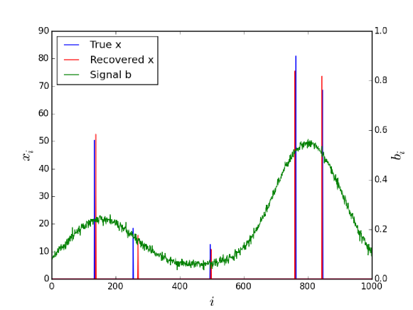
While not relevant to solving the optimization problem, the solution of the nonnegative deconvolution problem often, but not always, (approximately) recovers the original vector $\tilde{x}$. Figure 12 shows the solution recovered by ECOS [DCB13] for a problem instance with $n=1000$. The ECOS solution $x^{\star}$ had a cluster of 3-5 adjacent nonzero entries around each spike in $\tilde{x}$. The sum of the entries was close to the value of the spike. The recovered $x$ in figure 12 shows only the largest entry in each cluster, with value set to the sum of the cluster’s entries.

Figure 13: Solve time in seconds $T$ versus variable size $n$.

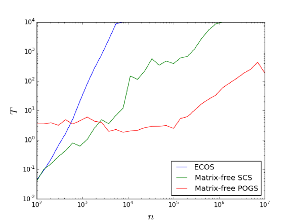
Results.

Figure 13 compares the performance on problem (1) of the interior-point solver ECOS [DCB13] and matrix-free versions of SCS and POGS as the size $n$ of the optimization variable increases. We limited the solvers to $10^{4}$ seconds.

For each variable size $n$ we generated ten different problem instances and recorded the average solve time for each solver. ECOS and matrix-free SCS were run with an absolute and relative tolerance of $10^{-3}$ for the duality gap, $\ell_{2}$ norm of the primal residual, and $\ell_{2}$ norm of the dual residual. Matrix-free POGS was run with an absolute tolerance of $10^{-4}$ and a relative tolerance of $10^{-3}$.

The slopes of the lines show how the solvers scale. The least-squares linear fit for the ECOS solve times has slope $3.1$, which indicates that the solve time scales like $n^{3}$, as expected. The least-squares linear fit for the matrix-free SCS solve times has slope $1.3$, which indicates that the solve time scales like the expected $n\log n$. The least-squares linear fit for the matrix-free POGS solve times in the range $n\in[10^{5},10^{7}]$ has slope $1.1$, which indicates that the solve time scales like the expected $n\log n$. For $n<10^{5}$, the GPU overhead (launching kernels, synchronization, etc.) dominates, and the solve time is nearly constant.

6.3 Sylvester LP

We applied our matrix-free convex optimization modeling system to Sylvester LPs, or convex optimization problems of the form

$$\begin{array}[]{ll}\mbox{minimize}&\mathop{\bf Tr}(D^{T}X)\\ \mbox{subject to}&AXB\leq C\\ &X\geq 0,\end{array}$$ (12)

where $X\in{\mbox{\bf R}}^{p\times q}$ is the optimization variable, and $A\in{\mbox{\bf R}}^{p\times p}$, $B\in{\mbox{\bf R}}^{q\times q}$, $C\in{\mbox{\bf R}}^{p\times q}$, and $D\in{\mbox{\bf R}}^{p\times q}$ are problem data. The inequality $AXB\leq C$ is a variant of the Sylvester equation $AXB=C$ [GLAM92].

Existing convex optimization modeling systems will convert problem (12) into the vectorized format

$$\begin{array}[]{ll}\mbox{minimize}&\mathop{\bf vec}(D)^{T}\mathop{\bf vec}(X)\\ \mbox{subject to}&(B^{T}\raisebox{1.0pt}{$\>\otimes\>$}A)\mathop{\bf vec}(X)\leq\mathop{\bf vec}(C)\\ &\mathop{\bf vec}(X)\geq 0,\end{array}$$ (13)

where $B^{T}\raisebox{1.0pt}{$\>\otimes\>$}A\in{\mbox{\bf R}}^{pq\times pq}$ is the Kronecker product of $B^{T}$ and $A$. Let $p=kq$ for some fixed $k$, and let $n=kq^{2}$ denote the size of the optimization variable. A standard interior-point solver will take $O(n^{3})$ flops and $O(n^{2})$ bytes of memory to solve problem (13). A specialized matrix-free solver that exploits the matrix product $AXB$, by contrast, can solve problem (12) in $O(n^{1.5})$ flops using $O(n)$ bytes of memory [VB95].

Problem instances.

We used the following procedure to generate interesting (nontrivial) instances of problem (12). We fixed $p=5q$ and generated $A$ and $B$ by first drawing entries i.i.d. from the folded standard normal distribution (i.e., the absolute value of the standard normal distribution). We then added $10^{-6}$ to all entries of $A$ and $B$ so they were guaranteed to be positive. We generated $D$ by drawing entries i.i.d. from a standard normal distribution. We fixed $C=11^{T}$. Our method of generating the problem data ensured the problem was feasible and bounded.

Figure 14: Solve time in seconds $T$ versus variable size $n$.

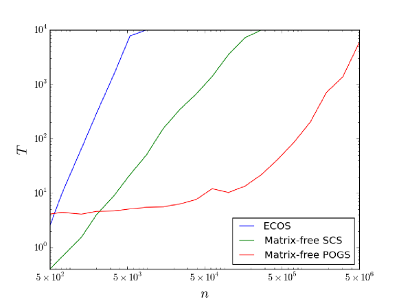
Results.

Figure 14 compares the performance on problem (12) of the interior-point solver ECOS [DCB13] and matrix-free versions of SCS and POGS as the size $n=5q^{2}$ of the optimization variable increases. We limited the solvers to $10^{4}$ seconds. For each variable size $n$ we generated ten different problem instances and recorded the average solve time for each solver. ECOS and matrix-free SCS were run with an absolute and relative tolerance of $10^{-3}$ for the duality gap, $\ell_{2}$ norm of the primal residual, and $\ell_{2}$ norm of the dual residual. Matrix-free POGS was run with an absolute tolerance of $10^{-4}$ and a relative tolerance of $10^{-3}$. The slope of the lines show how the solvers scale. The least-squares linear fit for the ECOS solve times has slope $3.3$, which indicates that the solve time scales like $n^{3}$, as expected. The least-squares linear fit for the matrix-free SCS solve times has slope $1.7$, which indicates that the solve time scales like the expected $n^{1.5}$. The least-squares linear fit for the matrix-free POGS solve times in the range $n\in[10^{5},5\times 10^{6}]$ has slope $1.6$, which indicates that the solve time scales like the expected $n^{1.5}$. For $n<10^{5}$, the GPU overhead (launching kernels, synchronization, etc.) dominates, and the solve time is nearly constant.

Appendix A Equivalence of the cone program

In this section we explain the precise sense in which the cone program output by the matrix-free canonicalization algorithm is equivalent to the original convex optimization problem.

Theorem A.1.

Let $p$ be a convex optimization problem whose OPR is a valid input to the matrix-free canonicalization algorithm. Let $\Phi(p)$ be the cone program represented by the output of the algorithm given $p$’s OPR as input. All the variables in $p$ are present in $\Phi(p)$, along with new variables introduced during the canonicalization process [Gra04, UMZ⁺14]. Let $x\in{\mbox{\bf R}}^{n}$ represent the variables in $p$ stacked into a vector and $t\in{\mbox{\bf R}}^{m}$ represent the new variables in $\Phi(p)$ stacked into a vector.

The problems $p$ and $\Phi(p)$ are equivalent in the following sense:

1. For all $x$ feasible in $p$, there exists $t^{\star}$ such that $(x,t^{\star})$ is feasible in $\Phi(p)$ and $p(x)=\Phi(p)(x,t^{\star})$.

2. For all $(x,t)$ feasible in $\Phi(p)$, $x$ is feasible in $p$ and $p(x)\leq\Phi(p)(x,t)$.

For a point $x$ feasible in $p$, by $p(x)$ we mean the value of $p$’s objective evaluated at $x$. The notation $\Phi(p)(x,t)$ is similarly defined.

Proof.

See [Gra04].    

Theorem A.1 implies that $p$ and $\Phi(p)$ have the same optimal value. Moreover, $p$ is infeasible if and only if $\Phi(p)$ is infeasible, and $p$ is unbounded if and only if $\Phi(p)$ is unbounded. The theorem also implies that any solution $x^{\star}$ to $p$ is part of a solution $(x^{\star},t^{\star})$ to $\Phi(p)$ and vice versa.

A similar equivalence holds between the Lagrange duals of $p$ and $\Phi(p)$, but the details are beyond the scope of this paper. See [Gra04] for a discussion of the dual of the cone program output by the canonicalization algorithm.

Appendix B Sparse matrix representation

In this section we explain the Matrix-Repr subroutine used in the standard canonicalization algorithm to obtain a sparse matrix representation of a cone program. Recall that the subroutine takes a list of linear expression DAGs, $(e_{1},\ldots,e_{\ell})$, and an ordering over the variables in the expression DAGs, $<_{V}$, as input and outputs a sparse matrix $A$.

The algorithm to carry out the subroutine is not discussed anywhere in the literature, so we present here the version used by CVXPY [DB]. The algorithm first converts each expression DAG into a map from variables to sparse matrices, representing a sum of terms. For example, if the map $\phi$ maps the variable $x\in{\mbox{\bf R}}^{n}$ to the sparse matrix coefficient $B\in{\mbox{\bf R}}^{m\times n}$ and the variable $y\in{\mbox{\bf R}}^{n}$ to the sparse matrix coefficient $C\in{\mbox{\bf R}}^{m\times n}$, then $\phi$ represents the sum $Bx+Cy$.

The conversion from expression DAG to map of variables to sparse matrices is done using algorithm 9. The algorithm uses the subroutine Matrix-Coeff, which takes a node representing a linear function $f$ and indices $i$ and $j$ as inputs and outputs a sparse matrix $D$. Let $\tilde{f}$ be a function defined on the range of $f$’s $i$th input such that $\tilde{f}(x)$ is equal to $f$’s $j$th output when $f$ is evaluated on $i$th input $x$ and zero-valued matrices (of the appropriate dimensions) for all other inputs. The output of Matrix-Coeff is the sparse matrix $D$ such that for any value $x$ in the domain of $\tilde{f}$,

$$D\mathop{\bf vec}(x)=\mathop{\bf vec}(\tilde{f}(x)).$$

The sparse matrix coefficients in the maps of variables to sparse matrices are assembled into a single sparse matrix $A$, as follows: Let $x_{1},\ldots,x_{k}$ be the variables in the expression DAGs, ordered according to $<_{V}$. Let $n_{i}$ be the length of $x_{i}$ if the variable is a vector and of $\mathop{\bf vec}(x_{i})$ if the variable is a matrix, for $i=1,\ldots,k$. Let $m_{j}$ be the length of expression DAG $e_{j}$’s output, for $j=1,\ldots,\ell$. The coefficients for $x_{1}$ are placed in the first $n_{1}$ columns in $A$, the coefficients for $x_{2}$ in the next $n_{2}$ columns, etc. Similarly, the coefficients from $e_{1}$ are placed in the first $m_{1}$ rows of $A$, the coefficients from $e_{2}$ in the next $m_{2}$ rows, etc.

Algorithm 9 Convert an expression DAG into a map from variables to sparse matrices.

$e$ is a linear expression DAG that outputs a single vector.

Create an empty queue $Q$ for nodes that are ready to evaluate.

Create an empty set $S$ for nodes that have been evaluated.

Create a map $M$ from (node, output index) tuples to maps of variables to sparse matrices.

for every start node $u$ in $e$ do

     $x\leftarrow$ the variable represented by node $u$.

     $n\leftarrow$ the length of $x$ if the variable is a vector and of $\mathop{\bf vec}(x)$ if the variable is a matrix.

     $M[(u,1)]\leftarrow$ a map with key $x$ and value the $n$-by-$n$ identity matrix.

     Add $u$ to $S$.

Add all nodes in $e$ to $Q$ whose only incoming edges are from start nodes.

while $Q$ is not empty do

     $u\leftarrow\text{pop the front node of }Q$.

     Add $u$ to $S$.

     for edge $(u,p)$ in $u$’s $E_{\mathrm{out}}$, with index $j$ do

         Create an empty map $M_{j}$ from variables to sparse matrices.

         for edge $(v,u)$ in $u$’s $E_{\mathrm{in}}$, with index $i$ do

              $A^{(ij)}\leftarrow\texttt{Matrix-Coeff}(u,i,j)$.

              $k\leftarrow$ the index of $(v,u)$ in $v$’s $E_{\mathrm{out}}$.

              for key $x$ and value $C$ in $M[(v,k)]$ do

                  if $M_{j}$ has an entry for $x$ then

                       $M_{j}[x]\leftarrow M_{j}[x]+A^{(ij)}C$.

                  else

                       $M_{j}[x]\leftarrow A^{(ij)}C$.                                          

         $M[(u,j)]\leftarrow M_{j}$.

         if for all edges $(q,p)$ in $p$’s $E_{\mathrm{in}}$, $q$ is in $S$ then

              Add $p$ to the end of $Q$.               

$u_{\mathrm{end}}\leftarrow$ the end node of $e$.

return $M[(u_{\mathrm{end}},1)]$.

References

- [ADV15] M. Andersen, J. Dahl, and L. Vandenberghe. CVXOPT: Python software for convex optimization, version 1.1. http://cvxopt.org/, May 2015.
- [Akl15] S. Akle. Algorithms for unsymmetric cone optimization and an implementation for problems with the exponential cone. PhD thesis, Stanford University, 2015.
- [ALSU06] A. Aho, M. Lam, R. Sethi, and J. Ullman. Compilers: Principles, Techniques, and Tools (2nd Edition). Addison-Wesley Longman Publishing Co., Inc., Boston, MA, USA, 2006.
- [ANR74] N. Ahmed, T. Natarajan, and K. Rao. Discrete cosine transform. IEEE Transactions on Computers, C-23(1):90–93, January 1974.
- [BCG11] S. Becker, E. Candès, and M. Grant. Templates for convex cone problems with applications to sparse signal recovery. Mathematical Programming Computation, 3(3):165–218, 2011.
- [BGH03] S. Börm, L. Grasedyck, and W. Hackbusch. Introduction to hierarchical matrices with applications. Engineering Analysis with Boundary Elements, 27(5):405–422, 2003.
- [BMR85] A. Brandt, S. McCormick, and J. Ruge. Algebraic multigrid (AMG) for sparse matrix equations. In D. Evans, editor, Sparsity and its Applications, pages 257–284. Cambridge University Press, Cambridge, 1985.
- [BPC+11] S. Boyd, N. Parikh, E. Chu, B. Peleato, and J. Eckstein. Distributed optimization and statistical learning via the alternating direction method of multipliers. Foundations and Trends in Machine Learning, 3:1–122, 2011.
- [Bra84] R. Bracewell. The fast Hartley transform. In Proceedings of the IEEE, volume 72, pages 1010–1018, August 1984.
- [Bré79] D. Brélaz. New methods to color the vertices of a graph. Communications of the ACM, 22(4):251–256, April 1979.
- [BT09a] A. Beck and M. Teboulle. Fast gradient-based algorithms for constrained total variation image denoising and deblurring problems. IEEE Transactions on Image Processing, 18(11):2419–2434, November 2009.
- [BT09b] A. Beck and M. Teboulle. A fast iterative shrinkage-thresholding algorithm for linear inverse problems. SIAM Journal on Imaging Sciences, 2(1):183–202, 2009.
- [BV04] S. Boyd and L. Vandenberghe. Convex Optimization. Cambridge University Press, 2004.
- [BY05] S. Benson and Y. Ye. DSDP5: Software for semidefinite programming. Technical Report ANL/MCS-P1289-0905, Mathematics and Computer Science Division, Argonne National Laboratory, Argonne, IL, September 2005. Submitted to ACM Transactions on Mathematical Software.
- [CDDY06] E. Candès, L. Demanet, D. Donoho, and L. Ying. Fast discrete curvelet transforms. Multiscale Modeling & Simulation, 5(3):861–899, 2006.
- [CDF92] A. Cohen, I. Daubechies, and J.-C. Feauveau. Biorthogonal bases of compactly supported wavelets. Communications on Pure and Applied Mathematics, 45(5):485–560, 1992.
- [CDS98] S. Chen, D. Donoho, and M. Saunders. Atomic decomposition by basis pursuit. SIAM Journal on Scientific Computing, 20(1):33–61, 1998.
- [CEN06] T. Chan, S. Esedoglu, and M. Nikolova. Algorithms for finding global minimizers of image segmentation and denoising models. SIAM Journal on Applied Mathematics, 66(5):1632–1648, 2006.
- [CGR88] J. Carrier, L. Greengard, and V. Rokhlin. A fast adaptive multipole algorithm for particle simulations. SIAM Journal on Scientific and Statistical Computing, 9(4):669–686, 1988.
- [CLW69] J. Cooley, P. Lewis, and P. Welch. The fast Fourier transform and its applications. IEEE Transactions on Education, 12(1):27–34, March 1969.
- [COPB13] E. Chu, B. O’Donoghue, N. Parikh, and S. Boyd. A primal-dual operator splitting method for conic optimization. Preprint, 2013. http://stanford.edu/~boyd/papers/pdf/pdos.pdf.
- [CP11] A. Chambolle and T. Pock. A first-order primal-dual algorithm for convex problems with applications to imaging. Journal of Mathematical Imaging and Vision, 40(1):120–145, May 2011.
- [CPDB13] E. Chu, N. Parikh, A. Domahidi, and S. Boyd. Code generation for embedded second-order cone programming. In Proceedings of the European Control Conference, pages 1547–1552. IEEE, 2013.
- [CT65] J. Cooley and J. Tukey. An algorithm for the machine calculation of complex Fourier series. Mathematics of computation, 19(90):297–301, 1965.
- [CY00] C. Choi and Y. Ye. Solving sparse semidefinite programs using the dual scaling algorithm with an iterative solver. Working paper, Department of Management Sciences, University of Iowa, 2000.
- [Dau88] I. Daubechies. Orthonormal bases of compactly supported wavelets. Communications on Pure and Applied Mathematics, 41(7):909–996, 1988.
- [Dau92] I. Daubechies. Ten lectures on wavelets, volume 61. SIAM, 1992.
- [Dav06] T. Davis. Direct Methods for Sparse Linear Systems (Fundamentals of Algorithms 2). SIAM, Philadelphia, PA, USA, 2006.
- [DB] S. Diamond and S. Boyd. CVXPY: A Python-embedded modeling language for convex optimization. Journal of Machine Learning Research. To appear.
- [DB15] S. Diamond and S. Boyd. Matrix-free convex optimization modeling. In Proceedings of the IEEE International Conference on Computer Vision, December 2015. To appear.
- [DCB13] A. Domahidi, E. Chu, and S. Boyd. ECOS: An SOCP solver for embedded systems. In Proceedings of the European Control Conference, pages 3071–3076, 2013.
- [DER86] I. Duff, A. Erisman, and J. Reid. Direct Methods for Sparse Matrices. Oxford University Press, Inc., New York, NY, USA, 1986.
- [DM84] D. Dudgeon and R. Mersereau. Multidimensional Digital Signal Processing. Prentice-Hall, Englewood Cliffs, NJ, USA, 1984.
- [DV03] M. Do and M. Vetterli. The finite ridgelet transform for image representation. IEEE Transactions on Image Processing, 12(1):16–28, January 2003.
- [FB15] C. Fougner and S. Boyd. Parameter selection and pre-conditioning for a graph form solver. Preprint, 2015. http://arxiv.org/pdf/1503.08366v1.pdf.
- [FFK+08] K. Fujisawa, M. Fukuda, K. Kobayashi, M. Kojima, K. Nakata, M. Nakata, and M. Yamashita. SDPA (semidefinite programming algorithm) user’s manual – version 7.0.5. Technical report, 2008.
- [FGZ12] K. Fountoulakis, J. Gondzio, and P. Zhlobich. Matrix-free interior point method for compressed sensing problems. Preprint, 2012. http://arxiv.org/pdf/1208.5435.pdf.
- [FKS02] M. Fukuda, M. Kojima, and M. Shida. Lagrangian dual interior-point methods for semidefinite programs. SIAM Journal on Optimization, 12(4):1007–1031, 2002.
- [FNW07] M. Figueiredo, R. Nowak, and S. Wright. Gradient projection for sparse reconstruction: Application to compressed sensing and other inverse problems. IEEE Journal of Selected Topics in Signal Processing, 1(4):586–597, December 2007.
- [FP02] D. Forsyth and J. Ponce. Computer Vision: A Modern Approach. Prentice Hall Professional Technical Reference, 2002.
- [FS11] D. Fong and M. Saunders. LSMR: An iterative algorithm for sparse least-squares problems. SIAM Journal on Scientific Computing, 33(5):2950–2971, 2011.
- [GB08] M. Grant and S. Boyd. Graph implementations for nonsmooth convex programs. In V. Blondel, S. Boyd, and H. Kimura, editors, Recent Advances in Learning and Control, Lecture Notes in Control and Information Sciences, pages 95–110. Springer, 2008.
- [GB14] M. Grant and S. Boyd. CVX: MATLAB software for disciplined convex programming, version 2.1. http://cvxr.com/cvx, March 2014.
- [GBY06] M. Grant, S. Boyd, and Y. Ye. Disciplined convex programming. In L. Liberti and N. Maculan, editors, Global Optimization: From Theory to Implementation, Nonconvex Optimization and its Applications, pages 155–210. Springer, 2006.
- [GLAM92] J. Gardiner, A. Laub, J. Amato, and C. Moler. Solution of the Sylvester matrix equation . ACM Transactions on Mathematical Software, 18(2):223–231, June 1992.
- [GO09] T. Goldstein and S. Osher. The split Bregman method for -regularized problems. SIAM Journal on Imaging Sciences, 2(2):323–343, 2009.
- [Gon12a] J. Gondzio. Convergence analysis of an inexact feasible interior point method for convex quadratic programming. Preprint, 2012. http://arxiv.org/pdf/1208.5960.pdf.
- [Gon12b] J. Gondzio. Matrix-free interior point method. Computational Optimization and Applications, 51(2):457–480, 2012.
- [GR87] L. Greengard and V. Rokhlin. A fast algorithm for particle simulations. Journal of Computational Physics, 73(2):325–348, 1987.
- [Gra04] M. Grant. Disciplined Convex Programming. PhD thesis, Stanford University, 2004.
- [GS91] L. Greengard and J. Strain. The fast Gauss transform. SIAM Journal on Scientific and Statistical Computing, 12(1):79–94, 1991.
- [GSTV07] A. Gilbert, M. Strauss, J. Tropp, and R. Vershynin. One sketch for all: Fast algorithms for compressed sensing. In Proceedings of the 39th Annual ACM Symposium on Theory of Computing, STOC ’07, pages 237–246, New York, NY, USA, 2007. ACM.
- [Hac85] W. Hackbusch. Multi-Grid Methods and Applications. Springer Berlin Heidelberg, 1985.
- [Hac99] W. Hackbusch. A sparse matrix arithmetic based on -matrices. Part I: Introduction to -matrices. Computing, 62(2):89–108, 1999.
- [Hal93] M. Halldórsson. A still better performance guarantee for approximate graph coloring. Information Processing Letters, 45(1):19–23, 1993.
- [HHS+14] G. Hennenfent, F. Herrmann, R. Saab, O. Yilmaz, and C. Pajean. SPOT: A linear operator toolbox, version 1.2. http://www.cs.ubc.ca/labs/scl/spot/index.html, March 2014.
- [HKS00] W. Hackbusch, B. Khoromskij, and S. Sauter. On 2-matrices. In H.-J. Bungartz, R. Hoppe, and C. Zenger, editors, Lectures on Applied Mathematics, pages 9–029. Springer Berlin Heidelberg, 2000.
- [HS52] M. Hestenes and E. Stiefel. Methods of conjugate gradients for solving linear systems. J. Res. N.B.S., 49(6):409–436, 1952.
- [JDCP11] L. Jacques, L. Duval, C. Chaux, and G. Peyré. A panorama on multiscale geometric representations, intertwining spatial, directional and frequency selectivity. IEEE Transactions on Signal Processing, 91(12):2699–2730, 2011.
- [JlCH01] A. Jensen and A. la Cour-Harbo. Ripples in Mathematics. Springer, 2001.
- [Kar72] R. Karp. Reducibility among combinatorial problems. In R. Miller, J. Thatcher, and J. Bohlinger, editors, Complexity of Computer Computations, The IBM Research Symposia Series, pages 85–103. Springer US, 1972.
- [KB77] P. Krishnaprasad and R. Barakat. A descent approach to a class of inverse problems. Journal of Computational Physics, 24(4):339–347, 1977.
- [Kha14] L. Khanh Hien. Differential properties of Euclidean projection onto power cone. http://www.optimization-online.org/DB_FILE/2014/08/4502.pdf, 2014.
- [KKL+07] S.-J. Kim, K. Koh, M. Lustig, S. Boyd, and D. Gorinevsky. An interior-point method for large-scale -regularized least squares. IEEE Journal on Selected Topics in Signal Processing, 1(4):606–617, December 2007.
- [KOSZ13] J. Kelner, L. Orecchia, A. Sidford, and A. Zhu. A simple, combinatorial algorithm for solving SDD systems in nearly-linear time. In Proceedings of the 45th Annual ACM Symposium on Theory of Computing, STOC ’13, pages 911–920, New York, NY, USA, 2013. ACM.
- [KS09] M. Koc̆vara and M. Stingl. On the solution of large-scale SDP problems by the modified barrier method using iterative solvers. Mathematical Programming, 120(1):285–287, 2009.
- [KV92] J. Kovacevic and M. Vetterli. Nonseparable multidimensional perfect reconstruction filter banks and wavelet bases for n. IEEE Transactions on Information Theory, 38(2):533–555, March 1992.
- [LD07] Y. Lu and M. Do. Multidimensional directional filter banks and surfacelets. IEEE Transactions on Image Processing, 16(4):918–931, April 2007.
- [Lib13] E. Liberty. Simple and deterministic matrix sketching. In Proceedings of the 19th ACM SIGKDD International Conference on Knowledge Discovery and Data Mining, pages 581–588, 2013.
- [Lim90] J. Lim. Two-dimensional Signal and Image Processing. Prentice-Hall, Inc., Upper Saddle River, NJ, USA, 1990.
- [LLM11] G. Lan, Z. Lu, and R. Monteiro. Primal-dual first-order methods with iteration-complexity for cone programming. Mathematical Programming, 126(1):1–29, 2011.
- [LLS04] Y. Lin, D. Lee, and L. Saul. Nonnegative deconvolution for time of arrival estimation. In Proceedings of the IEEE International Conference on Acoustics, Speech, and Signal Processing, volume 2, pages 377–380, May 2004.
- [Loa92] C. Van Loan. Computational Frameworks for the Fast Fourier Transform. SIAM, 1992.
- [Lof04] J. Lofberg. YALMIP: A toolbox for modeling and optimization in MATLAB. In Proceedings of the IEEE International Symposium on Computed Aided Control Systems Design, pages 294–289, September 2004.
- [Mal89] S. Mallat. A theory for multiresolution signal decomposition: the wavelet representation. IEEE Transactions on Pattern Analysis and Machine Intelligence, 11(7):674–693, July 1989.
- [Mar94] S. Martucci. Symmetric convolution and the discrete sine and cosine transforms. IEEE Transactions on Signal Processing, 42(5):1038–1051, May 1994.
- [MB12] J. Mattingley and S. Boyd. CVXGEN: A code generator for embedded convex optimization. Optimization and Engineering, 13(1):1–27, 2012.
- [mos15] MOSEK optimization software, version 7. https://mosek.com/, January 2015.
- [MZQ15] J. Miller, J. Zhu, and P. Quigley. Cvxcanon, version 0.0.22. https://github.com/cvxgrp/CVXcanon, October 2015.
- [Nes06] Y. Nesterov. Towards nonsymmetric conic optimization. http://www.optimization-online.org/DB_FILE/2006/03/1355.pdf, March 2006. CORE discussion paper.
- [NN92] Y. Nesterov and A. Nemirovsky. Conic formulation of a convex programming problem and duality. Optimization Methods and Software, 1(2):95–115, 1992.
- [NN94] Y. Nesterov and A. Nemirovskii. Interior-Point Polynomial Algorithms in Convex Programming, volume 13. SIAM, 1994.
- [NW06] J. Nocedal and S. Wright. Numerical Optimization. Springer Science, 2006.
- [OCPB15] B. O’Donoghue, E. Chu, N. Parikh, and S. Boyd. Conic optimization via operator splitting and homogeneous self-dual embedding. Preprint, 2015. http://stanford.edu/~boyd/papers/pdf/scs.pdf.
- [PB14] N. Parikh and S. Boyd. Proximal algorithms. Foundations and Trends in Optimization, 1(3):123–231, 2014.
- [PC11] T. Pock and A. Chambolle. Diagonal preconditioning for first order primal-dual algorithms in convex optimization. In Proceedings of the IEEE International Conference on Computer Vision, pages 1762–1769, 2011.
- [RKBA+13] J. Ragan-Kelley, C. Barnes, A. Adams, S. Paris, F. Durand, and S. Amarasinghe. Halide: A language and compiler for optimizing parallelism, locality, and recomputation in image processing pipelines. In Proceedings of the 34th ACM SIGPLAN Conference on Programming Language Design and Implementation, PLDI ’13, pages 519–530, New York, NY, USA, 2013. ACM.
- [SCD02] J.-L. Starck, E. Candès, and D. Donoho. The curvelet transform for image denoising. IEEE Transactions on Image Processing, 11(6):670–684, June 2002.
- [SKM+13] M. Saunders, B. Kim, C. Maes, S. Akle, and M. Zahr. PDCO: Primal-dual interior method for convex objectives. http://web.stanford.edu/group/SOL/software/pdco/, November 2013.
- [ST04] D. Spielman and S.-H. Teng. Nearly-linear time algorithms for graph partitioning, graph sparsification, and solving linear systems. In Proceedings of the 36th Annual ACM Symposium on Theory of Computing, STOC ’04, pages 81–90, New York, NY, USA, 2004. ACM.
- [Stu99] J. Sturm. Using SeDuMi 1.02, a MATLAB toolbox for optimization over symmetric cones. Optimization Methods and Software, 11(1-4):625–653, 1999.
- [SY14] A. Skajaa and Y. Ye. A homogeneous interior-point algorithm for nonsymmetric convex conic optimization. Mathematical Programming, pages 1–32, May 2014.
- [Toh04] K.-C. Toh. Solving large scale semidefinite programs via an iterative solver on the augmented systems. SIAM Journal on Optimization, 14(3):670–698, 2004.
- [TTT99] K.-C. Toh, M. Todd, and R. Tütüncü. SDPT3 — a MATLAB software package for semidefinite programming, version 4.0. Optimization Methods and Software, 11:545–581, 1999.
- [UMZ+14] M. Udell, K. Mohan, D. Zeng, J. Hong, S. Diamond, and S. Boyd. Convex optimization in Julia. SC14 Workshop on High Performance Technical Computing in Dynamic Languages, 2014.
- [Vai13] G. Vaillant. linop, version 0.7. http://pythonhosted.org//linop/, December 2013.
- [VB93] L. Vandenberghe and S. Boyd. A polynomial-time algorithm for determining quadratic Lyapunov functions for nonlinear systems. In Proceedings of the European Conference on Circuit Theory and Design, pages 1065–1068, 1993.
- [VB95] L. Vandenberghe and S. Boyd. A primal-dual potential reduction method for problems involving matrix inequalities. Mathematical Programming, 69(1-3):205–236, 1995.
- [vdBF09] E. van den Berg and M. Friedlander. Probing the Pareto frontier for basis pursuit solutions. SIAM Journal on Scientific Computing, 31(2):890–912, 2009.
- [Vis12] K. Vishnoi. Laplacian solvers and their algorithmic applications. Theoretical Computer Science, 8(1-2):1–141, 2012.
- [Wri87] S. Wright. Primal-Dual Interior-Point Methods, volume 54. SIAM, 1987.
- [YDC05] L. Ying, L. Demanet, and E. Candès. 3D discrete curvelet transform. In Proceedings of SPIE: Wavelets XI, volume 5914, pages 351–361, 2005.
- [YDD05] C. Yang, R. Duraiswami, and L. Davis. Efficient kernel machines using the improved fast Gauss transform. In L. Saul, Y. Weiss, and L. Bottou, editors, Advances in Neural Information Processing Systems 17, pages 1561–1568. MIT Press, 2005.
- [YDGD03] C. Yang, R. Duraiswami, N. Gumerov, and L. Davis. Improved fast Gauss transform and efficient kernel density estimation. In Proceedings of the IEEE International Conference on Computer Vision, volume 1, pages 664–671, October 2003.
- [Ye11] Y. Ye. Interior Point Algorithms: Theory and Analysis. Wiley-Interscience, 2011.
- [ZPB07] C. Zach, T. Pock, and H. Bischof. A duality based approach for realtime TV- optical flow. In Pattern Recognition, volume 4713 of Lecture Notes in Computer Science, pages 214–223. Springer Berlin Heidelberg, 2007.
- [ZST10] X.-Y. Zhao, D. Sun, and K.-C. Toh. A Newton-CG augmented Lagrangian method for semidefinite programming. SIAM Journal on Optimization, 20(4):1737–1765, 2010.