No evidence for multiple stellar populations in the low-mass Galactic globular cluster E 3

Abstract

Multiple stellar populations are a widespread phenomenon among Galactic globular clusters. Even though the origin of the enriched material from which new generations of stars are produced remains unclear, it is likely that self-enrichment will be feasible only in clusters massive enough to retain this enriched material. We searched for multiple populations in the low mass ($M\sim 1.4\times 10^{4}$ M_☉) globular cluster E 3, analyzing SOAR/Goodman multi-object spectroscopy centered on the blue CN absorption features of 23 red giant branch stars. We find that the CN abundance does not present the typical bimodal behavior seen in clusters hosting multi stellar populations, but rather a unimodal distribution that indicates the presence of a genuine single stellar population, or a level of enrichment much lower than in clusters that show evidence for two populations from high-resolution spectroscopy. E 3 would be the first bona fide Galactic old globular cluster where no sign of self-enrichment is found.

1. Introduction

Although the fact that globular clusters (GCs) are complex and not simple stellar populations has been widely acknowledge with the discovery of multiple stellar sequences in several clusters using high-precision photometry (e.g. Bedin et al., 2004; Piotto et al., 2007; Milone et al., 2008; Anderson et al., 2009) and the finding of a Sodium-Oxygen (NaO) anti-correlation in red giant branch (RGB) stars from high-resolution spectroscopy (e.g. Drake et al., 1992; Ivans et al., 2001; Gratton et al., 2001; Carretta et al., 2009b), star-to-star variations in the chemical composition of RGB stars and below, hinting at the existence of these multiple populations, have been known for a long time thanks to narrow-band imaging and low-resolution spectroscopy measuring the blue cyanogen (CN) bands (e.g. Osborn, 1971; Norris & Freeman, 1979; Norris et al., 1981; Bell et al., 1983).

With the exception of a few of the most massive Galactic GCs (Norris et al., 1996; Marino et al., 2011; Yong et al., 2014), GCs are homogeneous in iron-peak elements to within $\sim$0.1 dex (Carretta et al., 2009a; Willman & Strader, 2012), meaning that the pollution to the ISM necessary to produce distinct populations cannot come from supernovae. Instead, a number of other mechanisms have been discussed involving stellar winds from rotating low-metallicity stars (Maeder & Meynet, 2006), winds coming from Wolf-Rayet stars (Smith, 2006), massive interacting binaries (de Mink et al., 2009) polluting circumstellar discs of pre-main sequence stars (Bastian et al., 2013), or novae (Maccarone & Zurek, 2012), although the most heavily discussed mechanism is pollution by the ejecta of intermediate-mass asymptotic giant branch (AGB) stars (e.g. Cottrell & Da Costa, 1981; Ventura et al., 2001). In the case of clusters in the Magellanic Clouds, the presence of extended MS turn-offs (MSTO) in intermediate-age clusters has been interpreted as the presence of multiple stellar populations (e.g. Mackey et al., 2008), although this intepretation has been highly disputed (e.g. Bastian & Niederhofer, 2015; Brandt & Huang, 2015) Extended MSTOs are visible in clusters with masses down to $\sim 10^{4}M_{\sun}$ (Milone et al., 2009; Goudfrooij et al., 2011). Clusters below this limit would host single stellar populations (Conroy & Spergel, 2011).

Regardless of the origin of the enriched material, a key aspect is the ability to retain it in order to form new generations of stars. While the most massive clusters could retain SNe ejecta (e.g. $\omega$Cen), less massive GCs would retain only the more gentle outflows produced by the mechanisms mentioned above. This leads to the natural question of whether there is a mass limit below which no ejected material could be retained and hence genuine single-population GCs be produced (Caloi & D’Antona, 2011).

1.1. The low mass cluster E 3

E 3 (RA=09:20:57.07, Dec=–77:16:54.8 Goldsbury et al., 2010) is one of the sparsest ($r_{h}=4.94$ pc) and faintest GCs in our Galaxy (Lauberts, 1976). A metal-rich cluster ([Fe/H]=–0.74 Carretta et al., 2009b), is considered as part of the old GCs in our Galaxy (Marín-Franch et al., 2009), although its age could be as low as 2 Gyr less than 47 Tuc (Sarajedini et al., 2007), where the difficulties in establishing a precise age mostly stem from the uncertainties in its distance due to the lack of horizontal branch stars: while older measurements indicate a distance with $(m-M)_{0}=13.19$ (Harris, 1996), Sarajedini et al. (2007) measures a larger distance modulus of 14.54, value we adopt throughout this paper.

E 3 is also known for its very prominent binary star main sequence (McClure et al., 1985; Veronesi et al., 1996). Milone et al. (2012b) studied 59 Galactic GCs finding E 3 had the highest binary fraction in the sample.

Most relevant for this paper, E3 is among the lowest mass GCs in our Galaxy. With an apparent magnitude of $g=10.79$ (Vanderbeke et al., 2014) and a $M/L_{g}=2.83$ (for a 10 Gyr single stellar population using the Maraston 2005 models), E3 has a mass of $\sim 1.4\times 10^{4}$M_☉. Therefore, given its relatively short distance and low mass, E 3 provides one of the best targets to probe the existence of a mass limit for self-enrichment in Galactic GCs.

Finally, during the referee process of this paper, de la Fuente Marcos et al. (2015) presented high-resolution spectroscopy of 9 stars in the E 3 field, judging only two as cluster members based on the derived temperatures. From these two members, they find a radial velocity for the cluster $v_{r}=45\pm 5$ km s^-1, and based on thr proper motion of these two stars also derive a very high tangential velocity of $382\pm 79$ km s^-1. We discuss their radial velocity compared to our own measurement.

2. Observations and data reduction

2.1. SOAR/Goodman imaging

Optical imaging of E 3 was conducted with the Southern Astrophysical Research (SOAR) 4.1m telescope located in Cerro Pachón, Chile. The imaging mode of the Goodman spectrograph (Clemens et al., 2004) was used to obtain short exposures with each Kron-Cousins $B$ and $R$ filters on the night of October 1, 2013. Further $BV$ imaging was obtained on the night of January 14, 2015. Goodman provides a circular field of view of $7.2\arcmin$ in diameter in imaging mode.

Overscan subtraction, flat fielding and image alignment were applied with standard tools within iraf. FWHM measured on the combined images was $\sim 2.2\arcsec$ for the December 2013 images and $\sim 1\arcsec$ for the January 2015 run.

A catalog of sources produced with SExtractor (Bertin & Arnouts, 1996) was fed into daophot (Stetson, 1987) for measuring aperture photometry. Given the sparsity of the field, we found 5-pixel aperture photometry sufficient for our goals. Aperture corrections were established using 7 isolated secondary Stetson standards¹ which were also used to put magnitudes into the standard system. A color-magnitude diagram based on the January 2015 observations is shown in Fig. 1.

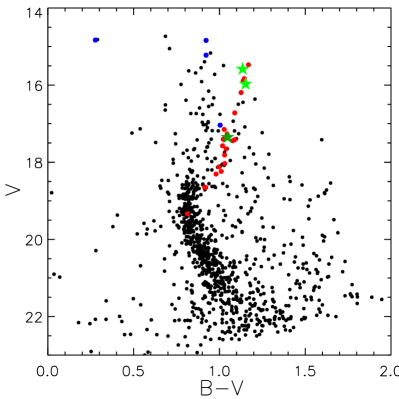
Figure 1.— $BV$ CMD of E 3. Member stars are indicated in red circles, while blue circles indicate stars judged as non-members based on their position in the CMD. The dark green star indicates the member star observed in both masks, while the light green star near the tip of the RGB were observed in a higher-resolution mode (Sect. 2.3)

2.2. SOAR/Goodman multi-object spectroscopy

Multi-object spectroscopy for selected sources was carried out during the commissioning run of the multi-object (MOS) capability of the Goodman spectrograph on the SOAR Telescope, during the night of December 18, 2013 (“mask 1”). Further observations were taken on February 17, 2015 (“mask 2”). Masks were prepared using the Slit Designer software developed at the University of North Carolina. An astrometric solution for the Goodman pre-images was found using the web-based tool astrometry.net² (Lang et al., 2010).

The Goodman MOS provides a fov of $3\arcmin\times 5\arcmin$. Mask 1 consisted of 13 slits, but only 12 stars could be extracted. Mask 2 had 14 slits covering 16 stars. Exposure times were $8\times 900$ s and $4\times 900$ s for masks 1 and 2, respectively. The 930 l$/$mm grating centered at 4100Å  was used for both masks, ensuring the presence of the CN 3883 Å  and 4215 Å  bands, CH 4300 Å  and Ca II H & K features in all spectra. H$\beta$ was also present in the wavelength range in most of the cases. Iron Argon comparison lamps were taken about every hour of observation. This setup gives a resolution of $\sim$ 2.7 Å  FWHM.

Standard reduction procedures were conducted using iraf. Wavelength calibration achieved an rms of $\sim 0.03$Å. Individual spectra were visually checked for defects before average. In the case of cosmic rays or other blemishes in the target wavelength ranges (see Sect. 3), the individual spectrum was removed before combination.

2.3. Radial velocities and SOAR longslit spectroscopy

As our observations were taken during commissioning of the Goodman multi-slit mode, the mask alignment was imperfect, and due to the blue wavelength range, no telluric absorption lines were present in the spectra to correct for the effects of slit miscentering. Therefore these spectra were unsuitable for the measurement of precise radial velocities.

To nail down the systemic velocity of the cluster, on 2015 June 13 we obtained a 600 sec longslit spectrum of two bright giants whose position in the color-magnitude diagram (light green stars in Fig. 1) suggested they were very likely to be cluster members. We used SOAR/Goodman with a 2400 l mm^-1 grating and a 1.03″slit, covering a wavelength range of $\sim 5100$–5600 Å at a resolution of about $0.75$ Å. The spectra were reduced in the standard manner and radial velocities derived through cross-correlation with spectra of bright stars of similar spectra type taken with the same setup.

The radial velocities of the two stars are consistent to within 4 km s^-1 and the mean heliocentric radial velocity is 8.9 $\pm$ 2.8 km s⁻¹. This velocity is in stark contrast with the velocity derived by de la Fuente Marcos et al. (2015), $v_{r}=45\pm 5$ km s^-1, which appeared during the referring process of this paper. Even though the cluster is known for undergoing tidal stripping (van den Bergh et al., 1980) and having a large binary fraction (Milone et al., 2012a), both factors that would increase the velocity dispersion of the cluster, the very marked difference between the two measurements suggests that one is not correct. This may be due to the presence of foreground stars in the sample. In the absence of additional information, we consider the systemic velocity of E3 to be uncertain. Fortunately, this issue can be easily settled with future high-resolution spectroscopy.

3. Index definition and measurements

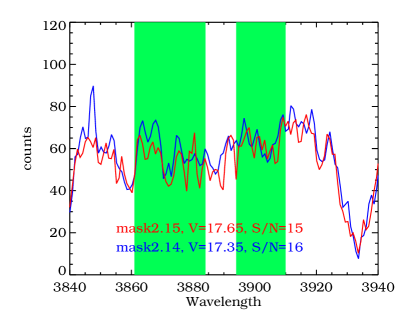
Figure 2.— The definition of the S(3839) index. The shaded region on the left shows the CN region, while the right shaded region is the adjacent continuum. The spectra of two stars with similar S/N is also shown.

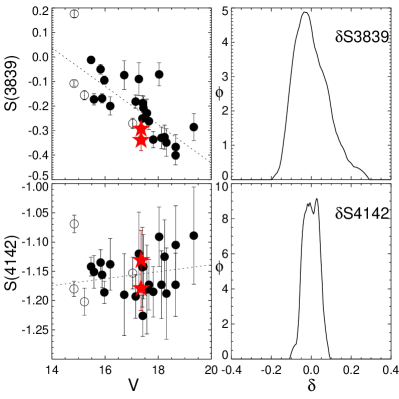
Figure 3.— $\rm{S}(3839)$ and $\rm{S}(4142)$ indices of RGB stars in E 3. Left panels show the uncorrected indices. Open symbols indicate non-member stars based on their CMD position. Red stars indicate duplicated measurements. Dashed lines indicate a robust linear fit to each distribution. Right panels indicate the density distribution of the corrected indices $\delta\rm{S}(3839)$ and $\delta\rm{S}(4142)$ .

CN and CH abundances (in rigor, line strenghts, although we will use the word abundance hereafter) were measured through spectral indices, which compare the flux value inside a window bracketing a spectral feature, with one or two adjacent windows which define a pseudo-continuum. We adopted the index definitions of Harbeck et al. (2003) in order to compare with other results from the literature (Sect. 4),

$$\rm{S}(3839) = -2.5\log{\frac{f_{3861-3884}}{f_{3894-3910}}},$$ (1)

$$\rm{S}(4142) = -2.5\log{\frac{f_{4120-4216}}{0.4\,f_{4055-4080}+0.6\,f_{4240-4280}}},$$ (2)

$$\rm{CH}(4300) = -2.5\log{\frac{f_{4285-4315}}{0.5\,f_{4240-4280}+0.5\,f_{4390-4460}}},$$ (3)

where each term is the sum of the flux in counts within the specified wavelength range. The uncertainties were measured assuming Poissonian noise for each flux measurement. Fig. 2 shows the definition of the S(3839) index over two sample spectra.

Figure 4.— Comparison of $\rm{S}(3839)$ and $\rm{S}(4142)$ indices. Median errors are depicted as bars in the lower right corner. While the $\rm{S}(3839)$ distribution is significantly broader than its median error, the $\rm{S}(4142)$ is consistent with its internal errors.

Table 1 shows the measured values and uncertainties for the indices $\rm{S}(3839)$ , $\rm{S}(4142)$ and CH(4300). Star 3 in the first mask was observed again as star 11 in the second mask (indicated with a star symbol in Figs. 1 and 3); the difference between the index measurements for this star is of the order of the calculated Poissonian errors, providing evidence for the consistency of our measurements between masks.

The intensities of the CN and CH indices are not only a function of chemical abundance, but also of temperature and gravity. To first order, these dependences can be removed using the proxies of color (Harbeck et al., 2003) or luminosity (e.g. Norris et al., 1981; Kayser et al., 2008), by fitting a curve to the lower envelope of the distribution (e.g. Harbeck et al., 2003) or by finding a ridge line that describes well the data (e.g. Pancino et al., 2010). In this case we adopt an approach similar to Pancino et al. (2010), by robust fitting of a straight line to the indices as function of $V$ magnitude (see Fig. 3). The right panels of Fig. 3 show the density distribution of the corrected indices, $\delta\rm{S}(3839)$ and $\delta\rm{S}(4142)$ , defined as the distance to the fitted line.

Even though the $\rm{S}(4142)$ feature is significantly weaker than the $\rm{S}(3839)$ (e.g. Norris et al., 1981), it benefits from having a $\sim$50% higher S/N (Table 1). The sensitivity and reliability of the indices can be tested by comparing the widths of their distributions to the measured errors. Fig. 4 shows the $\rm{S}(4142)$ index as function of $\rm{S}(3839)$ . While the spread in $\rm{S}(4142)$ values is consistent with the uncertainties, the spread in $\rm{S}(3839)$ is larger than the uncertainties, indicating a bigger sensitivity. Even though the $\rm{S}(4142)$ index shows a hint of bimodality (lower panels in Fig. 3), there are two reasons to discount it as not significant: first, the spread in the $\rm{S}(4142)$ index is consistent with that expected on the basis of the measurement uncertainties; second, the single star with multiple measurements “switches” between the two populations. Thus, while bimodality in $\rm{S}(4142)$ might well be present, we cannot claim its presence on the basis of these observations. Rather, we will focus the analysis on the stronger $\rm{S}(3839)$ index, as many studies before (e.g. Harbeck et al., 2003; Lardo et al., 2012; Lim et al., 2015).

4. Results

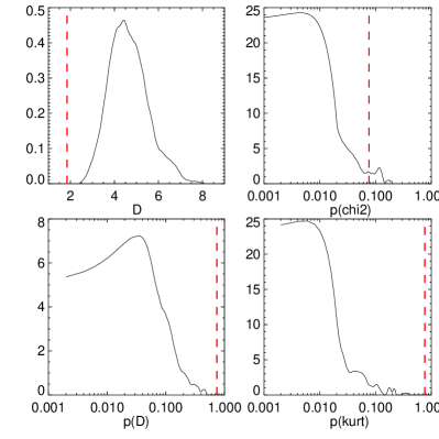
Figure 5.— GMM statistics for a “blurred” bimodal distribution where the peaks in the $\rm{S}(3839)$ distribution are separated by 0.25 mag (see text for details). For each statistic the vertical red dashed line indicates the GMM result for the original sample.

4.1. A unimodal CN abundance?

Fig. 3 (top right panel) shows the density distribution of the $\delta\rm{S}(3839)$ measurements, obtained using a kernel density estimator with an Epanechnikov kernel. The density distribution does not show obvious evidence for bimodality, but rather shows a behavior close to Gaussianity. To further test this visual impression, we use a Gaussian Mixture Modeling (GMM) as implemented by Muratov & Gnedin (2010). GMM makes a maximum likelihood estimation of the parameters associated with the selected number of Gaussians (two in this case), calculating uncertainties in these parameters via non-parametric bootstrap. It further calculates the distance between the peaks, $D=|\mu_{1}-\mu_{2}|/[(\sigma_{1}^{2}+\sigma_{2}^{2})/2]^{1/2}$, and the kurtosis of the sample. Finally, using a parametric bootstrap it calculates the probability that the observed distribution is drawn from a single Gaussian.

All the quantities measured by GMM are inconsistent with a bimodal distribution. GMM finds $D=1.85$, below $D=2$ which is considered as a clear separation between the peaks (Ashman et al., 1994) and a slightly negative kurtosis of $-0.102$, both quantities with probabilities 0.846 and 0.763 of being obtained from a unimodal distribution, respectively.

Is it possible that a true underlying bimodal distribution in $\rm{S}(3839)$ is hidden by observational errors and the relatively low S/N? We tested this hypothesis with two methods, generating a mock bimodal distribution, blurring it with the observational errors, and a second approach measuring the $\rm{S}(3839)$ index in SDSS spectra of the GC M71 with artificially reduced quality.

In the first method, we generated two random Gaussian distributions separated by a conservative $\Delta$ $\delta\rm{S}(3839)$ =0.25 mag (see below) and with $\sigma=0.06$ mag each, that is, slightly larger than the measured median uncertainty in the $\rm{S}(3839)$ values. The value of the separation between the input Gaussians is also smaller than the usual separation between CN-rich and CN-weak stars, which is close to 0.4 mag (e.g. Norris et al., 1981; Kayser et al., 2008; Lim et al., 2015). Each sample consisted of 23 objects randomly placed on either Gaussian. 200 samples were generated and run through GMM.

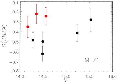
Figure 6.— CN abundance in the GC M 71. Filled symbols indicate the measured $\rm{S}(3839)$ on SDSS spectra (red circles indicating CN-rich stars), while error bars indicate the full range of values obtained from the same spectra when downgraded to S/N=10.

Fig. 5 shows the results of this exercise, where the vertical dashed lines represent the values obtained when GMM was applied to the original sample. The top left panel gives the distribution of distances between the peaks for the 200 generated bimodal samples. The peak separation is always higher than the observed value of 1.85. The three other panels show the probability of obtaining the measured $\chi^{2}$, peak distance and kurtosis from a unimodal distribution. These distributions are significantly different from the ones measured in the original sample, strongly rejecting bimodality with peak separations of 0.25 mag and above, and supporting a genuine unimodal distribution of the measured $\rm{S}(3839)$ values.

In the second method, we wanted to test directly the influence of low S/N in the reliability of the $\rm{S}(3839)$ index measurement. To this end, we retrieved SDSS/SEGUE (Yanny et al., 2009) spectra of 9 RGB stars belonging to the GC M71, which has a very similar metallicity to E 3, [Fe/H]$=-0.82$ (Carretta et al., 2009b). These data were already used by Smolinski et al. (2011), finding bimodality in the $\rm{S}(3839)$ index, using the Norris et al. (1981) definition, slightly different than the Harbeck et al. (2003) definition used throughout this paper. We downgraded the quality of the spectra to S/N=10 and measured the $\rm{S}(3839)$ index in 100 realizations of the original spectra with added noise. Fig. 6 shows the results of this approach. Solid circles show the measurements of the original spectra, while the error bars indicate the full range of measured values from the Montecarlo procedure. Despite the low number of stars and some confusion for the brightest stars, bimodality would remain clear under low S/N conditions.

Both methods show that a bimodal distribution with the separation expected for a metal-rich cluster will not become unimodal under relatively low S/N conditions, supporting the idea that the RGB of E 3 comprises a single stellar population.

5. Discussion.

Even though the CN bimodality has been found in a large number of clusters (e.g. Alves-Brito et al., 2008), clusters with no sign of a CN-rich population are not without precedent. Kayser et al. (2008) studied CN abundances in 8 GCs, finding that two of them, Terzan 7 and Palomar 12, do not present CN-rich stars. These two clusters are also anomalous in the sense that the widespread NaO anticorrelation is neither present (Sbordone et al., 2007; Cohen, 2004), although this result is based only on a handful of stars. Perhaps most importantly, both clusters are associated to the Sagittarius dwarf (e.g. Da Costa & Armandroff, 1995; Dinescu et al., 2000). This led Kayser et al. (2008) to suggest that the environment in which the clusters are formed would influence the presence of CN variations.

Another case is given by the low-metallicity cluster NGC 6397 ([Fe/H]$=-1.99$) which also serves as a cautionary tale: while no CN bimodality was found using low resolution spectra and narrow-band imaging (Lim et al., 2015), and also no multiple stellar populations were found using high quality multi-color ground-based photometry (Nardiello et al., 2015); high-precision HST photometry revealed the presence of two main sequences (Milone et al., 2012a). This apparent contradiction can be explained by the weaker CN absorption expected in low-metallicity clusters (e.g. Smolinski et al., 2011), which is not the case for E 3.NGC 6397 has also a well-studied Na-O anti-correlation (e.g. Gratton et al., 2001; Carretta et al., 2009b).

Based on detailed chemical abundances from high-resolution spectroscopy of 9 RGB stars, Villanova et al. (2013) claimed Ruprecht 106 as the first single-population cluster in our Galaxy. Even though its luminosity implies a larger present-day mass than E 3, Rup 106 is also regarded as a GC of extragalactic origin (Lin & Richer, 1992; Pritzl et al., 2005; Villanova et al., 2013). If environment plays a role in the generation of multiple stellar populations (Kayser et al., 2008), it is not unlikely the mass limit for self-enrichment will also be a function of environment.

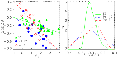
Figure 7.— A comparison between the $\delta\rm{S}(3839)$ distribution of E 3 and two clusters of similar metallicity, Terzan 7 and Palomar 12. The spread in the E 3 values is even narrower than in these two clusters considered as unimodal (Kayser et al., 2008).

5.1. A mass limit for self-enrichment?

Regardless of which mechanism expells processed material into the ISM in GCs, the potential of the cluster (and thus its mass and size) will determine how much material can be retained. Therefore it is likely that little or no material would be retained for self-enrichment below some cluster mass. The absence of abundance variations in the less massive open clusters (e.g. Norris & Smith, 1985; Martell & Smith, 2009; Carrera & Martínez-Vázquez, 2013; Bragaglia et al., 2014), is consistent with the existence of such a mass limit, though there may be other relevant factors, such as the physical conditions in the immediate environment of the forming cluster.

On the basis of the detailed abundances of a sample of 21 GCs and a comparison to open clusters, Carretta et al. (2010) suggest a limit of $M_{V}=-5.1$ (about $4\times 10^{4}M_{\sun}$ for an old stellar population), above which all GCs appear to show evidence of self-enrichment via the Na–O anti-correlation. This limit was chosen to separate the low mass GC Palomar 5 (which does show multiple populations) from the open clusters and the GCs Terzan 7 and Palomar 12, which do not show multiple populations. As mentioned before, besides their low masses, Terzan 7 and Palomar 12 also share an unusual characteristic, which is that they are much younger than the bulk of the Milky Way GC system and are inferred to have been accreted as part of the Sgr dwarf galaxy. Thus, it is unclear whether these GCs did not self-enrich because of their low masses and large sizes, or due to some other factor. We also note that E 3 is widely considered as a genuine Galactic cluster, not associated to any dwarf galaxy or stream (Forbes & Bridges, 2010). Carretta et al. (2010) consider it as a part of the disk/bulge subsystem of GCs based on its position inside the Galaxy.

In our view it is premature to make sweeping statements about the existence of a mass limit for self-enrichment. First, little data exists for low-mass GCs at all: there is a clear observational need to both improve data on E 3 (including high-resolution abundance measurements for bright giants) and to obtain low-resolution spectroscopy or medium-band photometry on other low-mass Milky Way GCs. One happy consequence of improved searches for satellites of the Milky Way has been the discovery of likely new low-mass GCs. The other problem is in interpretation. It is challenging to relate the present-day mass of an old, low-mass GC to its initial mass, though with improved Galactic models and cluster orbits from Gaia, the modeling of the mass loss from individual Milky Way GCs should be improved. A similar challenge exists for the initial structural parameters of the cluster, which can affect the central escape velocity at early times.

6. Summary and conclusions

We have presented SOAR/Goodman MOS spectroscopy of 23 RGB stars in the metal-rich, low-mass GC E3. We measured the blue CN absorption at 3883 Åfinding no evidence of an intrinsic spread in CN line strength. E3 is the first old Galactic GC consistent with a single stellar population.

Table 1Data for program stars

ID	$\alpha_{2000}$	$\delta_{2000}$	$V$	$(B-V)$	S(3839)	$\delta$$\rm{S}(3839)$	S/N	S(4142)	$\delta$$\rm{S}(4142)$	S/N	$\rm{CH}(4300)$	Member?
			mag	mag
m1.1	140.1972	-77.3133	15.224	0.922	–0.156$\pm$0.019	-0.097	24.6	–1.202$\pm$0.023	-0.035	38.6	1.009$\pm$0.019	N
m1.2	140.1748	-77.3129	14.832	0.277	–0.108$\pm$0.011	-0.080	64.5	–1.180$\pm$0.013	-0.010	90.6	1.005$\pm$0.011	N
m1.3	140.2880	-77.2892	17.354	1.047	–0.293$\pm$0.029	-0.063	13.8	–1.179$\pm$0.038	-0.024	22.4	1.056$\pm$0.032	Y
m1.4	140.2618	-77.2917	18.237	1.010	–0.327$\pm$0.049	-0.032	3.2	–1.125$\pm$0.063	0.024	7.5	1.048$\pm$0.053	Y
m1.5	140.2160	-77.2920	17.442	1.077	–0.208$\pm$0.046	0.024	8.1	–1.142$\pm$0.055	0.012	10.6	1.148$\pm$0.046	Y
m1.6	140.2543	-77.2762	17.150	1.028	–0.182$\pm$0.027	0.027	13.1	–1.193$\pm$0.037	-0.037	17.8	0.987$\pm$0.032	Y
m1.7	140.2197	-77.2771	18.120	0.997	–0.330$\pm$0.044	-0.045	4.2	–1.173$\pm$0.058	-0.023	7.9	1.024$\pm$0.048	Y
m1.8	140.1445	-77.2842	15.584	1.135	–0.173$\pm$0.023	-0.086	23.2	–1.151$\pm$0.028	0.014	35.5	1.072$\pm$0.023	Y
m1.9	140.1167	-77.2829	17.403	1.022	–0.251$\pm$0.058	-0.022	5.3	–1.143$\pm$0.068	0.011	7.4	1.048$\pm$0.056	Y
m1.10	140.1340	-77.2736	14.841	0.922	+0.176$\pm$0.015	0.205	50.7	–1.069$\pm$0.015	0.100	80.6	1.082$\pm$0.012	N
m1.11	140.1085	-77.2686	15.832	1.145	–0.050$\pm$0.020	0.056	18.8	–1.135$\pm$0.022	0.029	43.6	1.117$\pm$0.019	Y
m1.12	140.0702	-77.2658	15.889	1.138	–0.169$\pm$0.019	-0.058	24.8	–1.156$\pm$0.022	0.007	40.5	1.138$\pm$0.018	Y
m2.1	140.2114	-77.3321	17.270	1.045	–0.090$\pm$0.067	0.129	3.0	–1.120$\pm$0.071	0.035	10.3	1.139$\pm$0.058	Y
m2.2	140.1812	-77.3273	18.655	0.920	–0.367$\pm$0.050	-0.040	8.6	–1.105$\pm$0.067	0.042	13.5	0.995$\pm$0.057	Y
m2.3	140.1606	-77.3127	17.416	1.089	–0.188$\pm$0.031	0.042	18.6	–1.226$\pm$0.035	-0.072	31.0	1.041$\pm$0.029	Y
m2.4	140.1906	-77.3123	15.972	1.152	–0.095$\pm$0.017	0.022	43.8	–1.186$\pm$0.019	-0.023	68.6	1.188$\pm$0.016	Y
m2.5	140.2596	-77.3148	17.574	1.018	–0.229$\pm$0.057	0.014	8.2	–1.181$\pm$0.076	-0.028	11.8	1.003$\pm$0.062	Y
m2.6	140.2615	-77.3141	19.335	0.813	–0.286$\pm$0.055	0.095	6.2	–1.089$\pm$0.083	0.054	8.1	0.912$\pm$0.072	Y
m2.7	140.1342	-77.2990	15.474	1.169	–0.012$\pm$0.014	0.066	51.0	–1.142$\pm$0.016	0.024	81.7	1.146$\pm$0.013	Y
m2.8	140.1846	-77.2997	18.650	0.914	–0.401$\pm$0.039	-0.074	11.5	–1.173$\pm$0.054	-0.026	18.1	0.940$\pm$0.046	Y
m2.9	140.3156	-77.3011	16.194	1.126	–0.200$\pm$0.037	-0.065	20.3	–1.138$\pm$0.044	0.023	32.6	1.108$\pm$0.036	Y
m2.10	140.2847	-77.2912	18.306	0.980	–0.349$\pm$0.056	-0.049	6.0	–1.188$\pm$0.078	-0.039	10.7	1.042$\pm$0.065	Y
m2.11	140.2880	-77.2892	17.354	1.047	–0.339$\pm$0.043	-0.114	12.5	–1.131$\pm$0.051	0.024	19.8	1.125$\pm$0.043	Y
m2.12	140.3345	-77.2901	16.721	1.089	–0.074$\pm$0.058	0.102	9.0	–1.190$\pm$0.070	-0.032	13.4	1.056$\pm$0.056	Y
m2.13	140.2395	-77.2789	17.038	1.004	–0.271$\pm$0.021	-0.070	29.5	–1.153$\pm$0.027	0.003	43.5	1.025$\pm$0.023	N
m2.14	140.2739	-77.2794	17.812	1.030	–0.337$\pm$0.033	-0.076	16.0	–1.185$\pm$0.043	–0.033	24.2	1.039$\pm$0.036	Y
m2.15	140.2922	-77.2691	17.651	1.039	–0.262$\pm$0.034	-0.013	15.3	–1.173$\pm$0.043	–0.020	24.5	1.066$\pm$0.036	Y
m2.16	140.3223	-77.2586	18.033	1.031	–0.071$\pm$0.047	0.208	10.7	–1.091$\pm$0.051	0.059	18.2	1.095$\pm$0.043	Y

References

- Alves-Brito et al. (2008) Alves-Brito, A., Schiavon, R. P., Castilho, B., & Barbuy, B. 2008, A&A, 486, 941
- Anderson et al. (2009) Anderson, J., Piotto, G., King, I. R., Bedin, L. R., & Guhathakurta, P. 2009, ApJ, 697, L58
- Ashman et al. (1994) Ashman, K. M., Bird, C. M., & Zepf, S. E. 1994, AJ, 108, 2348
- Bastian et al. (2013) Bastian, N., Lamers, H. J. G. L. M., de Mink, S. E., et al. 2013, MNRAS, 436, 2398
- Bastian & Niederhofer (2015) Bastian, N., & Niederhofer, F. 2015, MNRAS, 448, 1863
- Bedin et al. (2004) Bedin, L. R., Piotto, G., Anderson, J., et al. 2004, ApJ, 605, L125
- Bell et al. (1983) Bell, R. A., Hesser, J. E., & Cannon, R. D. 1983, ApJ, 269, 580
- Bertin & Arnouts (1996) Bertin, E., & Arnouts, S. 1996, A&AS, 117, 393
- Bragaglia et al. (2014) Bragaglia, A., Sneden, C., Carretta, E., et al. 2014, ApJ, 796, 68
- Brandt & Huang (2015) Brandt, T. D., & Huang, C. X. 2015, ApJ, 807, 25
- Caloi & D’Antona (2011) Caloi, V., & D’Antona, F. 2011, MNRAS, 417, 228
- Carrera & Martínez-Vázquez (2013) Carrera, R., & Martínez-Vázquez, C. E. 2013, A&A, 560, A5
- Carretta et al. (2009a) Carretta, E., Bragaglia, A., Gratton, R., D’Orazi, V., & Lucatello, S. 2009a, A&A, 508, 695
- Carretta et al. (2010) Carretta, E., Bragaglia, A., Gratton, R. G., et al. 2010, A&A, 516, A55
- Carretta et al. (2009b) —. 2009b, A&A, 505, 117
- Clemens et al. (2004) Clemens, J. C., Crain, J. A., & Anderson, R. 2004, in Society of Photo-Optical Instrumentation Engineers (SPIE) Conference Series, Vol. 5492, Ground-based Instrumentation for Astronomy, ed. A. F. M. Moorwood & M. Iye, 331–340
- Cohen (2004) Cohen, J. G. 2004, AJ, 127, 1545
- Conroy & Spergel (2011) Conroy, C., & Spergel, D. N. 2011, ApJ, 726, 36
- Cottrell & Da Costa (1981) Cottrell, P. L., & Da Costa, G. S. 1981, ApJ, 245, L79
- Da Costa & Armandroff (1995) Da Costa, G. S., & Armandroff, T. E. 1995, AJ, 109, 2533
- de la Fuente Marcos et al. (2015) de la Fuente Marcos, R., de la Fuente Marcos, C., Moni Bidin, C., Ortolani, S., & Carraro, G. 2015, astro.ph::1507.01347
- de Mink et al. (2009) de Mink, S. E., Pols, O. R., Langer, N., & Izzard, R. G. 2009, A&A, 507, L1
- Dinescu et al. (2000) Dinescu, D. I., Majewski, S. R., Girard, T. M., & Cudworth, K. M. 2000, AJ, 120, 1892
- Drake et al. (1992) Drake, J. J., Smith, V. V., & Suntzeff, N. B. 1992, ApJ, 395, L95
- Forbes & Bridges (2010) Forbes, D. A., & Bridges, T. 2010, MNRAS, 404, 1203
- Goldsbury et al. (2010) Goldsbury, R., Richer, H. B., Anderson, J., et al. 2010, AJ, 140, 1830
- Goudfrooij et al. (2011) Goudfrooij, P., Puzia, T. H., Kozhurina-Platais, V., & Chandar, R. 2011, ApJ, 737, 3
- Gratton et al. (2001) Gratton, R. G., Bonifacio, P., Bragaglia, A., et al. 2001, A&A, 369, 87
- Harbeck et al. (2003) Harbeck, D., Smith, G. H., & Grebel, E. K. 2003, AJ, 125, 197
- Harris (1996) Harris, W. E. 1996, AJ, 112, 1487
- Ivans et al. (2001) Ivans, I. I., Kraft, R. P., Sneden, C., et al. 2001, AJ, 122, 1438
- Kayser et al. (2008) Kayser, A., Hilker, M., Grebel, E. K., & Willemsen, P. G. 2008, A&A, 486, 437
- Lang et al. (2010) Lang, D., Hogg, D. W., Mierle, K., Blanton, M., & Roweis, S. 2010, AJ, 139, 1782
- Lardo et al. (2012) Lardo, C., Milone, A. P., Marino, A. F., et al. 2012, A&A, 541, A141
- Lauberts (1976) Lauberts, A. 1976, A&A, 52, 309
- Lim et al. (2015) Lim, D., Han, S.-I., Lee, Y.-W., et al. 2015, ApJS, 216, 19
- Lin & Richer (1992) Lin, D. N. C., & Richer, H. B. 1992, ApJ, 388, L57
- Maccarone & Zurek (2012) Maccarone, T. J., & Zurek, D. R. 2012, MNRAS, 423, 2
- Mackey et al. (2008) Mackey, A. D., Broby Nielsen, P., Ferguson, A. M. N., & Richardson, J. C. 2008, ApJ, 681, L17
- Maeder & Meynet (2006) Maeder, A., & Meynet, G. 2006, A&A, 448, L37
- Maraston (2005) Maraston, C. 2005, MNRAS, 362, 799
- Marín-Franch et al. (2009) Marín-Franch, A., Aparicio, A., Piotto, G., et al. 2009, ApJ, 694, 1498
- Marino et al. (2011) Marino, A. F., Sneden, C., Kraft, R. P., et al. 2011, A&A, 532, A8
- Martell & Smith (2009) Martell, S. L., & Smith, G. H. 2009, PASP, 121, 577
- McClure et al. (1985) McClure, R. D., Hesser, J. E., Stetson, P. B., & Stryker, L. L. 1985, PASP, 97, 665
- Milone et al. (2009) Milone, A. P., Bedin, L. R., Piotto, G., & Anderson, J. 2009, A&A, 497, 755
- Milone et al. (2012a) Milone, A. P., Marino, A. F., Piotto, G., et al. 2012a, ApJ, 745, 27
- Milone et al. (2008) Milone, A. P., Bedin, L. R., Piotto, G., et al. 2008, ApJ, 673, 241
- Milone et al. (2012b) Milone, A. P., Piotto, G., Bedin, L. R., et al. 2012b, A&A, 540, A16
- Muratov & Gnedin (2010) Muratov, A. L., & Gnedin, O. Y. 2010, ApJ, 718, 1266
- Nardiello et al. (2015) Nardiello, D., Milone, A. P., Piotto, G., et al. 2015, A&A, 573, A70
- Norris et al. (1981) Norris, J., Cottrell, P. L., Freeman, K. C., & Da Costa, G. S. 1981, ApJ, 244, 205
- Norris & Freeman (1979) Norris, J., & Freeman, K. C. 1979, ApJ, 230, L179
- Norris & Smith (1985) Norris, J., & Smith, G. H. 1985, AJ, 90, 2526
- Norris et al. (1996) Norris, J. E., Freeman, K. C., & Mighell, K. J. 1996, ApJ, 462, 241
- Osborn (1971) Osborn, W. 1971, The Observatory, 91, 223
- Pancino et al. (2010) Pancino, E., Rejkuba, M., Zoccali, M., & Carrera, R. 2010, A&A, 524, A44
- Piotto et al. (2007) Piotto, G., Bedin, L. R., Anderson, J., et al. 2007, ApJ, 661, L53
- Pritzl et al. (2005) Pritzl, B. J., Venn, K. A., & Irwin, M. 2005, AJ, 130, 2140
- Sarajedini et al. (2007) Sarajedini, A., Bedin, L. R., Chaboyer, B., et al. 2007, AJ, 133, 1658
- Sbordone et al. (2007) Sbordone, L., Bonifacio, P., Buonanno, R., et al. 2007, A&A, 465, 815
- Smith (2006) Smith, G. H. 2006, PASP, 118, 1225
- Smolinski et al. (2011) Smolinski, J. P., Martell, S. L., Beers, T. C., & Lee, Y. S. 2011, AJ, 142, 126
- Stetson (1987) Stetson, P. B. 1987, PASP, 99, 191
- van den Bergh et al. (1980) van den Bergh, S., Demers, S., & Kunkel, W. E. 1980, ApJ, 239, 112
- Vanderbeke et al. (2014) Vanderbeke, J., West, M. J., De Propris, R., et al. 2014, MNRAS, 437, 1725
- Ventura et al. (2001) Ventura, P., D’Antona, F., Mazzitelli, I., & Gratton, R. 2001, ApJ, 550, L65
- Veronesi et al. (1996) Veronesi, C., Zaggia, S., Piotto, G., Ferraro, F. R., & Bellazzini, M. 1996, in Astronomical Society of the Pacific Conference Series, Vol. 92, Formation of the Galactic Halo…Inside and Out, ed. H. L. Morrison & A. Sarajedini, 301
- Villanova et al. (2013) Villanova, S., Geisler, D., Carraro, G., Moni Bidin, C., & Muñoz, C. 2013, ApJ, 778, 186
- Willman & Strader (2012) Willman, B., & Strader, J. 2012, AJ, 144, 76
- Yanny et al. (2009) Yanny, B., Rockosi, C., Newberg, H. J., et al. 2009, AJ, 137, 4377
- Yong et al. (2014) Yong, D., Roederer, I. U., Grundahl, F., et al. 2014, MNRAS, 441, 3396