The unusual radio afterglow of the ultra-long gamma-ray burst GRB 130925A

Abstract

GRB 130925A is one of the recent additions to the growing family of ultra-long GRBs (T90$\gtrsim 1000$ s). While the X-ray emission of ultra-long GRBs have been studied extensively in the past, no comprehensive radio dataset has been obtained so far. We report here the early discovery of an unusual radio afterglow associated with the ultra-long GRB 130925A. The radio emission peaks at low-frequencies ($\sim 7$ GHz) at early times, only $2.2$ days after the burst occurred. More notably, the radio spectrum at frequencies above $10$ GHz exhibits a rather steep cut-off, compared to other long GRB radio afterglows. This cut-off can be explained if the emitting electrons are either mono-energetic or originate from a rather steep, $dN/dE\propto E^{-4}$, power-law energy distribution. An alternative electron acceleration mechanism may be required to produce such an electron energy distribution Furthermore, the radio spectrum exhibits a secondary underlying and slowly varying component. This may hint that the radio emission we observed is comprised of emission from both a reverse and a forward shock. We discuss our results in comparison with previous works that studied the unusual X-ray spectrum of this event and discuss the implications of our findings on progenitor scenarios.

1. Introduction

Gamma-ray bursts (GRBs) are the most energetic explosions known in the Universe. These events exhibit prompt gamma-ray emission followed by what is referred to as afterglow emission in a wide range of wavelengths from X-rays to radio. Currently, GRBs are classified based on the duration of their prompt Gamma-ray emission. Short (duration $\lesssim 2$ s) and long (duration $\gtrsim 2$ s) bursts are believed to be a result of different progenitor systems (See reviews by Woosley & Bloom 2006; Nakar 2007; Berger 2014).

The common wisdom suggests that long GRBs originate from the core-collapse of massive stars (e.g., MacFadyen & Woosley 1999). Short GRBs, on the other hand, presumably arise from coalescence of two neutron stars (e.g., Paczynski 1986; Eichler et al. 1989). In these scenarios, the afterglow is explained by the fireball model (Piran 1999; Sari et al. 1999) where the broadband emission originates from electrons in the circumstellar (or interstellar) medium (CSM or ISM) which are accelerated by a forward shock driven by the relativistic ejecta. While many studies (see above) focus on understanding their origin, GRBs also serve as natural laboratories to study physical processes in extreme conditions, such as relativistic particle acceleration. In turn, understanding these processes and the conditions in which they occur can provide clues as to the true nature of GRBs. This paper is related only to GRBs with long prompt emission and thus we will discuss only this type of GRBs, hereafter.

Recently, Levan et al. (2014) have suggested that another class of high-energy transients may exist, with possibly a different progenitor system. They pointed out that a handful of GRBs exhibit very long prompt gamma-ray emission ($\geq 1000$ s). These events are usually followed by a late-time X-ray afterglow which shows flaring activity as late as $10^{4}$ s after the initial burst. Unlike other long GRB afterglows, the flaring activity in these ultra-long GRBs has especially high flux and longevity. Levan et al. suggest that these ultra-long GRBs may be a result of either a tidal disruption event (TDE) of a star by a black hole or a core-collapse of an extremely extended star (see also Gendre et al. 2013).

On 2013, September 25, another ultra-long GRB, namely GRB 130925A, was discovered (Lien et al. 2013). Both the X-ray and radio afterglows of this event show unique features. In this paper, we discuss the unusual radio emission of GRB 130925A and discuss the implications of its unique properties. We first summarize the details known so far from recent studies of this GRB in § 2. In § 3 we describe our radio observations and the data reduction. The data analysis and modeling is performed in § 4. We then discuss our findings in § 5 and summarize in § 6.

2. GRB 130925A - Discovery and recent studies

GRB 130925A was discovered by the Burst Alert Telescope (BAT; Barthelmy et al. 2005) onboard the Swift satellite (Gehrels et al. 2004). Golenetskii et al. (2013) reported that the prompt Gamma ray emission, observed by the Konus-wind satellite, lasted for $\sim 4500$ s and had a fluence of $5.0\pm 0.1\times 10^{-4}$ erg cm^-2. Adopting a redshift of $z=0.347$, as measured by Vreeswijk et al. (2013), results in isotropic energy of $E_{iso}\approx 1.5\times 10^{53}$ erg. Compared to other ultra-long GRBs (Levan et al. 2014), GRB 130925A is the nearest event discovered so far and the most energetic (see Table 1). The prompt Gamma-ray emission was followed by a spectacular X-ray emission with rapid flaring at the first $10^{4}$ seconds of the event. Once the flaring ceased, the X-ray emission decayed as a smooth power-law, typical of normal long GRBs at this stage. However, additional uncharacteristic properties of the X-ray emission have been revealed.

Table 1GRB 130925A in comparison to previously discovered ultra-long GRBs

Name	$z$	$E_{iso}$	$T_{90}$
		[erg]	[sec]
GRB 101225A	0.85	$1.2\times 10^{52}$	$>7000$
GRB 111209A	0.67	$5.2\times 10^{52}$	$\sim 10,000$
GRB 101225A	1.77	$7\times 10^{52}$	$\sim 6000$
GRB 130925A	0.35	$1.5\times 10^{53}$	$\sim 4500$

Notes - The properties of the previously discovered GRBs are adopted from Levan et al. (2014).

Bellm et al. (2014) analysed the X-ray data obtained by the Swift, NuSTAR, and the Chandra satellites. Surprisingly, they found that the X-ray spectrum in the energy range $1-20$ keV, can not be modeled with a single power-law, as in essentially most normal long GRB afterglows to date (however, see Starling et al. 2012, that report a thermal X-ray component in some GRBs associated with SNe) . Bellm et al. obtained satisfactory fits to the observed X-ray spectrum with several models including: 1. two power-law components; 2. a power-law $+$ an absorption line at $~{}6$ keV; 3. a power-law and a blackbody component. However, the physical interpretation of the models was inconclusive. Recently, Piro et al. (2014) analyzed additional X-ray data from the XMM space observatory. According to their analysis, the X-ray emission is dominated by a blackbody emission and that only a small contribution of the X-ray emission is due to non-thermal synchrotron emission from a traditional afterglow (an afterglow from an external forward shock). A different explanation for the late-time X-ray emission was suggested by Evans et al. (2014). They argue that the emission is a result of reflection from dust which resides far away from the GRB. Both Piro et al. (2014) and Evans et al. (2014) find that the lack of (or weak) X-ray emission from the external shock suggests an extremely low circumburst density ($n\leq 0.1\,{\rm cm}^{-3}$).

In the optical regime, Greiner et al. (2014) reported the detection of a flare, $300-400$ s after the prompt emission. At late-times, Tanvir et al. (2013) observed GRB 130925A with the Hubble Space Telescope (HST). They detected an optical afterglow with an offset of 0$\farcs 12$ from the host galaxy center. This offset may disfavor a TDE scenario for this event. However, Tanvir et al. also note that the host galaxy is disrupted and that this may be a sign of a recent merger. In this case, it is possible that a massive black hole can be offset from the optical light center, thus still leaving a TDE as a plausible scenario.

3. VLA observations of GRB 130925A

We observed GRB 130925A with the Karl G. Jansky Very Large Array (VLA) under a Director Discretionary Time (DDT) program (14A-435; PI Horesh). Our observations consist of multi-epoch observations starting $2.2$ days after the burst. Each observation was performed using a varying set of average frequencies: $3.4$ GHz (S-band), $6.1$ GHz (C-band), $9$ GHz (X-band), $14.75$ GHz (Ku-band), and $22$ GHz (K-band). The various observing epochs (starting on 2013 Sep 27 UT; see Table 2) were performed with the VLA being either in the A or B configuration.

In all of our VLA observations, we used 3C48 as a flux calibrator and J0240-2309 as a phase calibrator. The data were then reduced using both AIPS and CASA (McMullin et al. 2007) standard routines. To estimate the accuracy of our flux calibration and to check for any calibration errors we compare the measured flux of our phase calibrator at the various observing epochs. The wide-band spectra of the phase calibrator at different times are consistent within the following wide-band flux calibration errors: $6.3\%$, $1.3\%$, $2.5\%$, $5\%$, and $5\%$ in the S-, C-, X-, Ku, and K-bands, respectively. Note that these calibration errors were calculated when using the full bandwidth in each band (2-8 GHz bandwidth) and have been adjusted for sub-band measurements. The full set of our measurements is presented in Table 2.

Table 2Summary of JVLA radio observations of GRB 130925A

Time	Frequency	Flux	Flux r.m.s
days	[GHz]	[$\mu$Jy]	[$\mu$Jy]
2	4.8	237	17
2	7.4	298	12
2	9.5	293	14
2	13.5	146	20
2	16.0	89	22
2	22.0	104	13
9	4.8	216	14
9	7.4	214	9
9	8.5	180	10
9	9.5	203	10
43	3.0	133	27
43	4.8	105	13
43	7.4	87	10
43	13.5	60	9
43	16.0	62	9
43	22.0	83	8
58	3.0	99	27
58	4.8	77	15
58	7.4	68	15
58	8.5	65	14
58	9.5	56	15
58	14.75	46	11
74	3.0	83	6
74	6.1	71	6
74	9.0	56	5
74	14.75	42	8
94	3.4	59	13
94	6.1	47	7
94	9.0	34	7
94	14.75	33	7
94	22.0	33	8
108	3.5	39	12
108	6.1	50	6
108	9.0	41	6
108	14.75	44	6
108	22.0	38	10
499	6.1	$<24$	–
499	9.0	$<24.3$	–

Notes - Time is given in days in days since the burst. The errors presented in the table represent the rms error from each image. When given, limits are $3\sigma$ detection limits. Systematic flux calibration errors were added according to §2. Both the rms error and the calibration should be combined in quadrature.

4. Radio Spectrum Analysis

Figure 1 shows the observed wide-band radio spectra at different epochs. The spectrum from the first epoch, $2.2$  days after discovery, shows that the emission is already peaking at low frequencies ($\sim 7$ GHz) and that it is strikingly cut off at $\geq 10$ GHz. Both these properties are not typical of normal GRB radio afterglows (see Chandra & Frail 2012 for a review of GRB radio afterglow properties), in particular the high-frequency cut off.

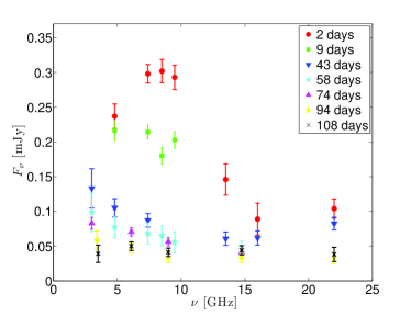
Figure 1.— Radio spectra of GRB 130925A at various VLA observation epochs. The initial spectrum shows a peculiar cut off at frequency $\geq 10$ GHz. Moreover, the spectral evolution suggest the existence of an underlying (and slowly variable) constant-flux component. However, more than a year after its discovery, the radio emission from GRB 130925A faded away below our detection limit (See Table 2).

Before discussing the implication of the high-frequency emission cut off, we test whether this cut off can be due to some modulation of the intrinsic flux via extreme interstellar scattering and scintillation (ISS). According to Cordes & Lazio (2002), the Galactic scattering measure (SM) towards the position of the GRB is ${\rm log}\,SM\approx-3.69~{}[{\rm kpc~{}m}^{-20/3}]$. The transition frequency from strong to weak scintillation is at $\approx 8$ GHz. At higher frequencies only small ISS flux modulations are expected. Thus it is unlikely that the observed cut off in the radio emission above $10$ GHz, is due to temporal strong scintillation (i.e., expected modulation $\lesssim 10\%$). Moreover, even at frequencies below the transition frequency (i.e., the strong scattering regime), we do not observe strong scintillation (see § 4.3.3).

In the context of the fireball afterglow model (see § 1), GRB afterglow spectra are usually well described by a broken power-law (Sari et al. 1998). This is a result of the radio emitting electrons being accelerated into a power-law energy distribution, $dN/dE\propto E^{-p}$. The spectral behavior depends on some characteristic frequencies, which define the transition between the different spectral slopes (see a detailed description by Sari et al. 1998). In short, at lower frequencies, the emission will be optically thick. At frequencies where the emission becomes optically thin, the specific flux will rise as $\nu^{1/3}$ up to some maximum value after which the specific flux will decay as $\nu^{-(p-1)/2}$. At even higher frequencies, beyond some cooling frequency (which usually occurs at or above the optical regime, at early times), the specific flux has a steeper decline of $\nu^{-p/2}$.

The typical average observed value of the electron energy power-law distribution is $p\approx 2$ (e.g., Panaitescu & Kumar 2001), but with a relatively wide distribution of $\sigma_{p}\approx 0.5$ (Shen, Kumar & Robinson 2006). Thus, typically, the spectral slope of the optically thin radio emission, above the peak frequency but below the cooling frequency, is rather shallow ($\nu^{-0.5}$). The sharp spectral cut off we observe in the case of GRB 130925A, raises the possibility that the power-law energy distribution of the emitting electrons is much steeper than in any other observed GRB to date. Another possibility is that an alternative model is required, such as a mono-energetic energy distribution. We next test both models by performing a minimum $\chi^{2}$ fitting to the data.

4.1. The power-law energy distribution model

Here we fit the initial observed radio spectrum with the common power-law afterglow model, consisting of an optically thick synchrotron self-absorbed emission ($\nu^{5/2}$) and an optically thin emission which has a power-law spectral shape ($\nu^{-\beta}$). Since, as seen in Figure 1, the radio emission appears to be decaying into a flat spectrum, it is possible that there is an additional slowly varying flat spectrum emitting component which we treat as constant over the time scale of our observations. Therefore, we perform the model fitting both with and without a second constant flux component.

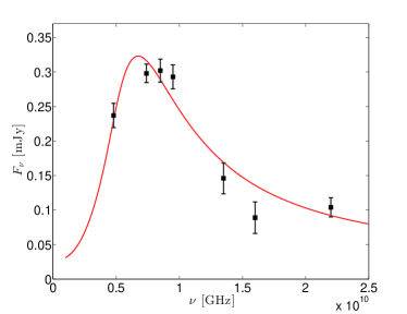
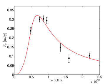
Figure 2.— Best fit of the power-law model to the observed initial radio spectrum. The two fits are with (left panel) and without (right panel) an additional constant flux component ($27\mu$Jy). Both fits suggest a steep electron energy distribution, not previously observed in GRBs (see text for details).

Figure 2 shows the best fit results. The fit without a constant flux component has a reduced $\chi^{2}$, i.e. $\chi^{2}$ per degrees of freedom (d.o.f), of $\chi^{2}_{\nu}=4.2$ (d.o.f $=3$). Adding a second component of constant flux to the fit results in a $\chi^{2}_{\nu}=6.2$ (d.o.f $=2$). The best fit spectral indexes in the former and latter fits are $s=1.4\pm 0.1$ and $s=1.6\pm 0.2$, respectively. Assuming that $s=(p-1)/2$, suggests that the electron energy distribution power-law indexes are $p\approx 3.8$ and $p\approx 4.2$, respectively. These are rather steep energy distributions, not observed so far in GRB radio afterglows.

4.2. A mono-energetic synchrotron emission

Motivated by the sharp cut off observed in the initial radio spectrum, we next consider an alternative model in which the observed synchrotron emission originates from relativistic electrons with a mono-energetic energy distribution. Since this model is rarely used for GRB afterglows (however see Waxman $\&$ Loeb 1999), we next describe it in more detail.

The synchrotron emission from a single electron is

$$P_{\nu}(\nu)=\frac{\sqrt{3}q_{e}^{3}B}{m_{e}c^{2}}F\left(\frac{\nu}{\nu_{c}}\right)$$ (1)

in the shockwave frame, where $c$ is the speed of light, $B$ is the magnetic field strength, $q_{e}$ and $m_{e}$ are the electron charge and mass, respectively, and

$$F(x)=x\int_{x}^{\infty}K_{5/3}\left(\zeta\right)d\zeta,$$ (2)

where $K$ is the modified Bessel function. The synchrotron frequency, $\nu_{synch}$ is defined as

$$\nu_{synch}=\frac{3\gamma_{e}^{2}q_{e}B}{4\pi m_{e}c},$$ (3)

where $\gamma_{e}$ is the Lorenz factor of the electrons (in the shockwave frame). In the relativistic case, the emission measured by an observer will be beamed and therefore in the observer frame the emission is

$$P_{\nu,{\rm beamed}}(\nu)=\Gamma\frac{\sqrt{3}q_{e}^{3}B}{m_{e}c^{2}}F\left(\frac{\nu}{\nu_{synch}}\right),$$ (4)

where $\Gamma$ is the bulk Lorentz factor of the shockwave. The frequency $\nu_{synch}$ in the observer frame will be the same as above multiplied by a factor of $\Gamma$.

In the case where internal synchrotron self-absorption (SSA) is dominant, the observed specific luminosity in the shockwave frame will be

$$L_{SSA}(\nu)=\frac{4\pi R^{3}}{\eta}P_{\nu}\left(\frac{1-e^{-\tau_{SSA}}}{\tau_{SSA}}\right).$$ (5)

Here, we assumed a planar absorption and the optical depth is defined as

$$\tau_{SSA}=\alpha_{SSA}\frac{R}{\eta},$$ (6)

where $\alpha_{SSA}$ is the absorption coefficient defined as (Rybicki & Lightman 1986):

$$\alpha_{SSA}=-\frac{c}{8\pi m_{e}\nu^{2}}\int\frac{N(E)}{E^{2}}\frac{d}{dE}\left[E^{2}P_{\nu}\right]dE,$$ (7)

where $N(E)$ is the volumetric density of electrons with energy $E=\gamma_{e}m_{e}c^{2}$.

The shape of a SSA spectrum therefore depends also on the energy distribution of the electrons, $N(E)$. In the mono-energetic case, $N(E)=N_{0}\delta(E-E_{0})$ (also assuming constant spatial density). In this case, equation $7$ is reduced to:

$$\alpha_{SSA}=-\frac{c^{2}}{8\pi\nu^{2}}\left[N_{0}\left.\frac{dP_{\nu}}{dE}\right|_{E_{0}}+\frac{2P_{\nu}(E_{0})N_{0}}{E_{0}}\right].$$ (8)

The specific flux in this case can therefore be easily calculated using the following properties: $B$, $\gamma_{e}$, $n_{e}$, and $R$.

Finally, the observed flux can be reduced to the simple form (see Waxman & Loeb 1999):

$$f_{\nu}=A\nu^{2}\zeta\left(\frac{\nu}{\nu_{synch}}\right),$$ (9)

where

$$\zeta\equiv\frac{1-e^{-\tau_{\nu}}}{1-[d\,ln\,F(x)/d\,ln\,x]},$$ (10)

$$A\equiv 4\pi\gamma_{e}m_{e}(R/D_{L})^{2},$$ (11)

and $D_{L}$ is the luminosity distance.

As in § 4.1, we performed the model fitting twice, with and without an additional constant flux component. The fitting of these two cases resulted in $\chi^{2}_{\nu}=1.7$ (d.o.f $=2$) and $\chi^{2}_{\nu}=6.2$ (d.o.f $=3$), respectively, where the best fits are presented in Figure 3. From a $\chi^{2}$ point of view, the mono-energetic model with a secondary constant flux component is slightly preferable (although not significantly) to the power-law model from § 4.1.

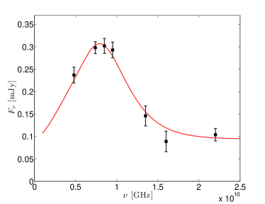
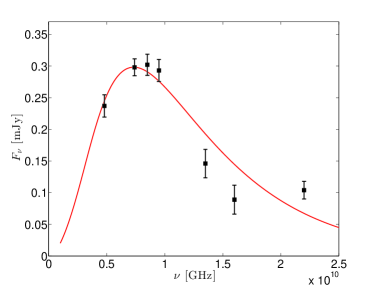
Figure 3.— Best fit of the mono-energetic model to the observed initial radio spectrum. The two fits are with (left panel) and without (right panel) an additional constant flux component ($95\mu$Jy). The mono-energetic + a constant flux component provide the best fit to the data.

4.3. Properties of the emitting medium

We derive the electron density, the magnetic field strength and the radius of the emitting regions for two cases: 1. An isotropic sub relativistic emitting sphere. 2. Emission from a relativistic jet.

4.3.1 The sub relativistic isotropic case

Here we assume that by the time of the observation the bulk motion is sub relativistic, and that the emission is isotropic. In addition we also assume some ratio between the energy density of the electrons ($E_{e}$) to the energy density of the magnetic field ($E_{B}$). Adopting the preferred model of mono-energetic electrons and assuming equipartition ($E_{e}=E_{B}$), the best fit to the data at the first observing epoch requires a radius of $R_{iso}\approx 8.5\times 10^{16}$ cm, a large electron density of $n_{e}\approx 400$ cm^-3 with $\gamma_{e}\approx 45$, and a magnetic field strength of $B\approx 0.61$  Gauss. The minimum required energy in this scenario is quite large, $E_{min}\approx 2.3\times 10^{49}$ erg. The fact that we observe only the optically thin synchrotron emission from the third epoch and on does not allow us to obtain estimates of the above model parameters in these additional epochs.

4.3.2 A Relativistic Jet

Recently, Barniol Duran, Nakar & Piran (2013), presented a straightforward method for calculating the above properties if the emission is originating from a relativistic jet. Adopting their prescriptions and assuming equipartition we derive the values of the emitting region properties using our measurements of the peak flux and frequency at our initial epoch of observation. We find that, at that time, the jet is only mildly relativistic with a bulk Lorentz factor of $\Gamma\approx 4$. The Jet radius is $R_{jet}\approx 1.3\times 10^{17}$  the electron density (assuming constant density) $n_{e}\approx 11$ cm^-3, the magnetic field strength is $B\approx 0.05$ G, the electron Lorenz factor is $\gamma_{e}\approx 245$, and the minimum kinetic energy is $E_{k}\approx 1.7\times 10^{47}{\rm erg}$. The relatively low value of $\Gamma$ should not be surprising given that the initial Lorentz factor is estimated to be $\Gamma_{0}\sim 20-37$ (Greiner et al. 2013).

4.3.3 A constraint on source size via scintillation

As was already discussed above, radio flux variations, especially at low frequencies, can be observed due to ISS. The ISS flux modulations depends on the angular size of the emitting source. In turn, the detection or lack of such modulations can be used to constrain the source size. In our initial observing epoch, we observed the source at 4.8 GHz twice within $\sim 2$ hours. We did not detect any strong variation in the source flux between these two observations. Thus we assume that the ISS modulations are within our measurement errors. Conservatively, we estimate then that the ISS modulation is $\leq 20\%$. Using the equations from Walker (1998) for refractive and diffractive scintillation, we find that the source angular size should be $\geq 3\times 10^{17}$ cm (radius $\geq 1.5\times 10^{17}$ cm), comparable to the source size we derived above.

5. Discussion

5.1. Electron energy distribution

In § 4 we found that the energy distribution of the radio emitting electrons can be fitted with either a very steep power-law or a mono-energetic energy distribution. None of these distributions have been observed in GRB radio afterglows to date. Previously observed GRB afterglows have exhibited a power-law energy distribution with a power-law index of $p\approx 2$. Theoretical studies (see Piran 2004 and references therein) suggest that electrons are accelerated at the GRB shock front via the Fermi process into a power-law distribution with a power-law index of $p\approx 2.2-2.3$, in agreement with past observations. A steep spectrum is possible if the synchrotron cooling frequency is below the observed frequency. However, the best fit of each of the two models in § 4.3 results in a cooling frequency of $\nu_{c}>10^{12}$ Hz, well above the observed radio frequencies. Thus producing the observed steep energy distribution may require an alternative particle acceleration mechanism. Another recent challenge for current particle acceleration models in GRBs has been made by Wiersema et al. (2014) who detected circular polarization in the optical afterglow of GRB 121024A.

Mono-energetic electrons have been observed in other astrophysical sources, such as the galactic center (Lesch & Reich 1992; Duschl & Lesch 1994). In solar flares, the initial particle acceleration is believed to be a result of magnetic reconnection which creates a mono-energetic soft X-rays emission (see Benz 2008 for a review). Moreover, some solar flares also exhibit steep optically thin radio spectra (e.g. Nita, Gary, & Lee 2004). Magnetic reconnection in accretion disks has also been suggested, as a possible explanations for intra-day variability in AGNs and Blazars (e.g., Lesch & Phol 1992; Crusius-Waetzel & Lesch 1998). Can magnetic reconnection be involved in the case of GRB 130925A? While this question remains open, certain aspects of it are already being addressed by ongoing studies (e.g., Sironi & Spitkovsky 2014)

5.2. The origin of the radio emission and its connection to the X-rays

The radio emission from most long GRBs is believed to originate from a forward shock in an external medium. If the radio emission of GRB 130925A is indeed originating from a forward shock then the properties found in § 4.3 are the properties of the ISM (or CSM). We test whether the observed X-ray emission can arise from a simple forward shock afterglow model, using the best fit parameters we derived from the radio data. In this case, extrapolating the steep power-law (or mono energetic) synchrotron emission into the X-ray bandpass results in a low flux, orders of magnitudes below the observed emission reported by Bellm et al. (2013), Piro et al. (2014), and Evans et al. (2014) (expected $\nu F_{\nu}$ of $\sim 10^{-20}$ erg cm^-2 s^-1 compared to the observed one of $\sim 10^{-12}$ erg cm^-2 s^-1).

Both Piro et al. and Evans et al. suggest that there is only a weak (or no) contribution from a forward shock to the observed X-ray emission. Instead they provide different explanations for that emission, such as blackbody radiation or scattering of the prompt emission by dust. Both Piro et al. and Evans et al. conclude then that the CSM density must be very low, with $n\leq 0.1\,{\rm cm}^{-3}$. In contrast, we find that, if the radio emission originates from a forward shock, then the lack of non-thermal X-ray emission is not due to low CSM density but rather due to the unusual steep energy distribution of the emitting electrons. In fact the electron density we find is higher by a factor of more than an order of magnitude than that of Piro et al. (2014) and Evans et al. (2014).

Alternatively, it is possibile that the radio emission is the result of a reverse shock ploughing through the dense ejecta. In this scenario, the electron density we find is that of the expanding ejecta shell. This renders the comparison between the electron density we derive and the low density CSM environment found by Evans et al. and Piro et al., irrelevant. In this scenario, the underlying weaker component that is observed in the radio spectrum may originate from the forwards shock. In fact, a second component of $F_{\nu}\propto\nu^{1/3}$, instead of a constant flat spectrum one, is also consistent with the data. Thus the existence of this second component makes the reverse shock scenario more plausible. However, if this second component is not from forward shock emission, it means that the afterglow from the forward shock is suppressed. As was already discussed by Evans et al., one way to surpress forward shock emission is by invoking a very weak magnetic field in the forward shock, compared to the one in the shocked ejecta. Alternatively, this can also be achieved by reducing the kinetic energy to less than $10^{50}{\rm erg}$, an energy budget which is still in agreement with the minimum kinetic energy we find in § 4.3. The reverse shock scenario, however, cannot explain the fact the we still see emission, above the secondary constant flux component, at $43$ days. Any emission from a reverse shock is expected to decrease by at least $1-2$ orders of magnitude compared to the emission observed at early times. Thus, our observations at late-times hampers the reverse shock scenario.

The question, though, what is the origin of the X-ray emission, still remains. If we put the implications of the radio data aside, a forward shock as an explanation for the X-ray emission becomes unlikely also when comparing the emission at a wavelength of $2.2\mu{\rm m}$ (Greiner et al. 2014) to the X-ray flux, two days after discovery. The ratio between the two implies a relatively low spectral index between $-0.3$ to $-0.6$, while we expect a steeper spectrum due to the transition beyond the cooling frequency. In fact, the shockwave parameters derived by Piro et al. suggest a $2.2\mu{\rm m}$ emission much higher than the observed one.

It is possible, in some cases, to produce X-ray emission via the inverse-Compton (IC) process. For example, a large enough reservoir of optical photons can be easily up-scattered to X-rays by electrons with a Lorentz factor of $\gamma_{e}\sim 50$. This possibility is especially intriguing since both the radio and the X-ray spectrum exhibit similar steep spectral slopes. Using the measurements of Greiner et al. as an estimate for the available optical and infrared photons, we find that the expected IC X-ray emission is $\nu F_{\nu}\sim 5\times 10^{-14}\,{\rm erg}\,{\rm cm}^{-2}\,{\rm s}^{-1}$. The observed X-ray emission, therefore, can not be accounted for by IC, since it is higher by almost two orders of magnitude than the expected IC emission.

Another possibility is that the X-ray emission originates from a different process and region in the progenitor system, than the radio emission. As already mentioned, Piro et al. suggest that most of the X-ray emission is blackbody emission originating from a compact radius of $10^{11}$ cm. This radius is much smaller than that of the radio emitting region. In contrast, in the Evans et al. model the X-ray echoing dust lies far away at pc scales. At the same time, one can argue that the fact that the emission at both radio and X-ray exhibit an unusual steep spectrum, may suggest a common origin. Additional analysis of the observed X-ray emission is beyond the scope of this work.

5.3. Implications for the nature of the progenitor

As GRB 130925A belongs to the ultra-long GRB subclass, we consider the two main progenitor scenarios suggested for this class, namely a TDE or an extreme collapsar. One of the best examples of a relativistic TDE is SwiftJ 1644+57 (Levan et al. 2011; Bloom et al. 2011; Burrows et al. 2011). Comparing the radio properties of SwiftJ 1644+57 (Zauderer et al. 2011; Berger et al. 2012) to GRB 130925A we find significant differences. First, SwiftJ 1644+57 was more radio luminous, by a factor of $>50$ than GRB 130925A. Second, the radio spectrum peak of SwiftJ 1644+57 traversed below $10$ GHz only at very late times, after $300$ days. Furthermore, the external medium surrounding SwiftJ 1644+57, is much denser. Overall, the radio properties of SwiftJ 1644+57 do not resemble in any way those of GRB 130925A. This, of course, is not proof that GRB 130925A is not a TDE, as SwiftJ 1644+57 is the first discovery of an onset of a TDE, but its properties may not be representative of the the whole population of relativistic TDEs. Beyond the comparison of the properties of GRB 130925A to the one of the Swift 1644+57, the properties of the former do not meet the expectations of theoretical TDE models. According to Giannios & Metzger (2011), the minimal rise time of the radio flux will be $t_{rise}\approx 30-200$ days, depending on the black hole mass. In contrast, the peak radio emission of GRB 130925A is already declining between 2 to 9 days, after discovery.

The radio emission does not pose a clear challenge to the collapsar scenario. The radio can be explained as either a forward or a reverse shock in this scenario. However, Piro et al. have suggested that the progenitor is a blue super giant (BSG) star with very little or no mass-loss. If the radio is originating from a forward shock, then a denser CSM than the one found by Piro et al. is required. Thus a progenitor with such low mass-loss as the one suggested by Piro et al. is not possible. On the other hand, the reverse shock case does not present a contradiction to the BSG progenitor scenario.

In both of the above progenitor models, the spectral cut off in the radio, has to be explained, especially since it was not observed before in TDEs or normal long GRBs (collapsars). In fact, the unique radio spectrum that may require an alternative electron acceleration mechanism, may, in turn, point to a different progenitor system that has not been considered so far. For example, in § 5.1, we speculated that magnetic reconnection may be the mechanism responsible for the acceleration of the radio emitting electrons. Singh et al. (2014) have studied the role of magnetic reconnection in accretion disk systems from micro-quasar scales to blazars. They found that fast reconnection originating from the central core, can play a part in the main energy output of these type of objects. At the same time, they found that this core mechanism cannot explain the energy output of GRBs and that the afterglow emission may arise from a more distant location, such as the jet. However, there is a suggestion by Giannios (2013) that magnetic reconnection may take place in jets as well. Can it be that GRB 130925A is in fact not related to either a collapsar or a TDE event? Another piece of the puzzle is that the radio spectrum slowly decays to a flat spectrum in $\sim 100$ days. Can this be a hint that this event is actually related to an AGN activity? Assuming so, the minimum variability time of $\approx 1$ s in the prompt emission (Greiner et al. 2014), suggest a BH mass of $<10^{5}\,{\rm M}_{\odot}$. This low mass disfavors the AGN scenario. Moreover, $\sim 1.5$ years after the GRB discovery, the seemingly constant flat radio emission component has disappeared.

6. Summary

We report here for the first time, the early radio observation and detection of an ultra-long GRB, GRB 130925A. The early radio spectrum obtained $2.2$ days after the burst, has some unusual properties. First, the radio emission peaks at $\sim 7$ GHz, already at early times. Even more surprising is the sharp spectral cut off at $>10$ GHz. We find that the data can be fitted with a SSA emission model in which the emission originates from either mono-energetic electrons or an electron population with an unusually steep power-law energy distribution. This may require an alternative acceleration mechanism other than the one usually used in relativistic shock models of GRBs.

Having unusual properties in various wavelengths, GRB 130925A may be of a completely different nature than other GRBs. There is no clear concise scenario that describes the overall properties of this particular GRB. Certainly the usual fireball scenario used to explain long GRBs does not capture the whole picture as the different pieces of the puzzle (radio, optical and X-rays) cannot necessarily be put together in this picture.

In the overall scheme of ultra-long GRBs, it seems that our radio data provides another evidence that differentiates this type of events from other normal long GRBs. However, since this is the first detailed early radio spectrum obtained for an ultra-long GRB, it is not clear whether GRB 130925A is representative of the ultra-long GRB population as a whole. Still, GRB 130925A raises some interesting questions regarding the properties and the progenitor nature of ultra-long GRBs. One example, is the fact that ultra-long GRBs exhibit steep X-ray spectra. Margutti et al. (2014) explains this by invoking dust echoes on parsec scales, similar to the explanation of Evans et al. (2014) in the case of GRB 130925A. Is it accidental that both the X-ray and radio spectra are soft? Or maybe the X-ray and radio emission are originally connected to particles accelerated by the same mechanism? These are open questions that we hope to find answers to in future panchromatic (radio to X-ray) studies of ultra-long GRBs.

References

- Barniol Duran, Nakar, & Piran (2013) Barniol Duran R., Nakar E., Piran T., 2013, ApJ, 772, 78
- Barthelmy et al. (2005) Barthelmy S. D., et al., 2005, SSRv, 120, 143
- Bellm et al. (2014) Bellm E. C., et al., 2014, ApJ, 784, LL19
- Benz (2008) Benz A. O., 2008, LRSP, 5, 1
- Berger et al. (2012) Berger E., Zauderer A., Pooley G. G., Soderberg A. M., Sari R., Brunthaler A., Bietenholz M. F., 2012, ApJ, 748, 36
- Berger (2014) Berger E., 2014, ARA&A, 52, 43
- Bloom et al. (2011) Bloom J. S., et al., 2011, Sci, 333, 203
- Burrows et al. (2011) Burrows D. N., et al., 2011, Natur, 476, 421
- Chandra & Frail (2012) Chandra P., Frail D. A., 2012, ApJ, 746, 156
- Cordes & Lazio (2002) Cordes J. M., Lazio T. J. W., 2002, astro, arXiv:astro-ph/0207156
- Crusius-Waetzel & Lesch (1998) Crusius-Waetzel A. R., Lesch H., 1998, A&A, 338, 399
- Duschl & Lesch (1994) Duschl W. J., Lesch H., 1994, A&A, 286, 431
- Eichler et al. (1989) Eichler D., Livio M., Piran T., Schramm D. N., 1989, Natur, 340, 126
- Evans et al. (2014) Evans P. A., et al., 2014, MNRAS, 444, 250
- Gehrels et al. (2004) Gehrels N., et al., 2004, ApJ, 611, 1005
- Gendre et al. (2013) Gendre B., et al., 2013, ApJ, 766, 30
- Giannios & Metzger (2011) Giannios D., Metzger B. D., 2011, MNRAS, 416, 2102
- Giannios (2013) Giannios D., 2013, MNRAS, 431, 355
- Golenetskii et al. (2013) Golenetskii S., Aptekar R., Frederiks D., Pal’Shin V., Oleynik P., Ulanov M., Svinkin D., Cline T., 2013, GCN, 15260, 1
- Greiner et al. (2014) Greiner J., et al., 2014, A&A, 568, AA75
- Lesch & Reich (1992) Lesch H., Reich W., 1992, A&A, 264, 493
- Lesch & Pohl (1992) Lesch H., Pohl M., 1992, A&A, 254, 29
- Levan et al. (2011) Levan A. J., et al., 2011, Sci, 333, 199
- Levan et al. (2014) Levan A. J., et al., 2014, ApJ, 781, 13
- Lien et al. (2013) Lien A. Y., Markwardt C. B., Page K. L., Palmer D. M., Racusin J. L., Siegel M. H., Ukwatta T. N., 2013, GCN, 15246, 1
- MacFadyen & Woosley (1999) MacFadyen A. I., Woosley S. E., 1999, ApJ, 524, 262
- Margutti et al. (2014) Margutti R., et al., 2014, arXiv, arXiv:1410.7387
- McMullin et al. (2007) McMullin, J. P., Waters, B., Schiebel, D., Young, W., Golap, K. 2007, Astronomical Data Analysis Software and Systems XVI (ASP Conf. Ser. 376), ed. R. A. Shaw, F. Hill, D. J. Bell (San Francisco, CA: ASP), 127
- Nakar (2007) Nakar E., 2007, PhR, 442, 166
- Nita, Gary, & Lee (2004) Nita G. M., Gary D. E., Lee J., 2004, ApJ, 605, 528
- Ofek (2014) Ofek E. O., 2014, ascl.soft, 1407.005
- Paczynski (1986) Paczynski B., 1986, ApJ, 308, L43
- Panaitescu & Kumar (2001) Panaitescu A., Kumar P., 2001, ApJ, 560, L49
- Piran (2004) Piran T., 2004, RvMP, 76, 1143
- Piran (1999) Piran T., 1999, PhR, 314, 575
- Piro et al. (2014) Piro L., et al., 2014, ApJ, 790, LL15
- Sari, Piran, & Narayan (1998) Sari R., Piran T., Narayan R., 1998, ApJ, 497, L17
- Sari & Piran (1999) Sari R., Piran T., 1999, ApJ, 517, L109
- Shen, Kumar, & Robinson (2006) Shen R., Kumar P., Robinson E. L., 2006, MNRAS, 371, 1441
- Sironi & Spitkovsky (2014) Sironi L., Spitkovsky A., 2014, ApJ, 783, LL21
- Starling et al. (2011) Starling R. L. C., et al., 2011, MNRAS, 411, 2792
- Starling et al. (2012) Starling R. L. C., Page K. L., Pe’Er A., Beardmore A. P., Osborne J. P., 2012, MNRAS, 427, 2950
- Rybicki & Lightman (1986) Rybicki G. B., Lightman A. P., 1986, rpa..book,
- Vreeswijk et al. (2013) Vreeswijk P. M., Malesani D., Fynbo J. P. U., De Cia A., Ledoux C., 2013, GCN, 15249, 1
- Walker (1998) Walker M. A., 1998, MNRAS, 294, 307
- Waxman & Loeb (1999) Waxman E., Loeb A., 1999, ApJ, 515, 721
- Wiersema et al. (2014) Wiersema K., et al., 2014, Natur, 509, 201
- Woosley & Bloom (2006) Woosley S. E., Bloom J. S., 2006, ARA&A, 44, 507
- Tanvir et al. (2013) Tanvir N. R., Levan A. J., Hounsell R., Fruchter A. S., Cenko S. B., Perley D. A., O’Brien P. T., 2013, GCN, 15489, 1
- Zauderer et al. (2011) Zauderer B. A., et al., 2011, Natur, 476, 425