Possible golden events for ringdown gravitational waves

Abstract

There is a forbidden region in the parameter space of quasinormal modes of black holes in general relativity. Using both inspiral and ringdown phases of gravitational waves from binary black holes, we propose two methods to test general relativity. We also evaluate how our methods will work when we apply them to Pop III black-hole binaries with typical masses. Adopting the simple mean of the estimated range of the event rate, we have the expected rate of 500 ${\rm yr^{-1}}$. Then, the rates of events with signal-to-noise ratios greater than 20 and greater than 50 are 32 ${\rm yr^{-1}}$ and 2 ${\rm yr^{-1}}$, respectively. Therefore, there is a good chance to confirm (or refute) the Einstein theory in the strong gravity region by observing the expected quasinormal modes.

I Introduction

Black hole (BH) singularities appear unavoidably in general relativity (GR). However, as a physics law the allowance of the presence of singularities will not be acceptable even though they are hidden behind the event horizon. Therefore, various possibilities of the singularity avoidance have been discussed. Some replacement of singularities is required as a complete theory which can describe the BH evolution inside the horizon. Although it is totally unknown how the singularities are to be regularized, there are a lot of proposals motivated by the string theory and/or the BH information paradox. Some of them, such as gravastars Mazur:2001fv , fuzzballs (see, e.g., Ref. Mathur:2005zp for the review) and firewalls Braunstein:2009my ; Almheiri:2012rt change the structure of BH spacetime even outside the horizon. Also, an interesting class of singularity and ghost free theories of gravity has been proposed by Ref. Modesto:2011kw ; Biswas:2011ar .

In this paper, we consider binary black hole (BBH) systems, and use gravitational wave (GW) observations as a tool to test whether the newly formed black hole genuinely behaves like the one predicted by GR or not. There are various methods proposed for testing GR by means of quasinormal mode (QNM) GWs (see an extensive review Berti:2015itd ), for example, tests of the no-hair theorem combining two or more modes Dreyer:2003bv . QNMs dominate the GWs at the ringdown phase of BBH mergers (see also Ref. Berti:2009kk ). In Ref. Hughes:2004vw , testing Hawking’s area theorem Hawking:1971tu has been discussed, which is possible if we can determine the masses and spins of BHs before and after merger independently with a sufficiently high accuracy.

One of the methods that we propose in this paper is the following simple one. First, we extract the binary parameters of BBHs by taking correlation with the post-Newtonian (PN) templates Blanchet:2013haa ; Schafer:2009dq . We assume that we know sufficiently high PN-order terms to describe the inspiral phase well. Thanks to the development in numerical relativity (NR) Pretorius:2005gq ; Campanelli:2005dd ; Baker:2005vv , now we can use simulation results to describe the BBH merger phase, deriving accurate gravitational waveforms. Next, if GR is correct, after the merger phase we will observe ringdown (QNM) GWs from the remnant BHs (see, e.g., Ref. Berti:2009kk for a review of the QNMs). If we do not detect the QNMs as expected, it is possible to distinguish the remnant object from the BHs that are predicted by GR within the assumptions mentioned above. It should be noted that our approach is similar to Ref. Luna:2006gw , in which the authors discussed the improvement in parameter estimation by combining inspiral and ringdown GWs from compact binaries. By contrast, the focus of our work is on the test of GR.

The other method shown in this paper is even simpler. When we focus on the dominant QNM, there is a forbidden parameter region in GR. Just using the ringdown GWs, we can directly discuss whether the QNM from the remnant compact object is consistent with the one from a BH predicted by GR or not.

This paper is organized as follows. In Sec. II, we summarize our tools, the inspiral and ringdown waveforms from BBHs, the fitting formulas for the remnant mass and spin, and the matched filtering and parameter estimation in the GW data analysis. In Sec. III, two simple tests of GR are presented. One is to use only the ringdown GWs, and the other is the combination of inspiral and ringdown phases. Finally, we summarize and discuss our approach in Sec. IV. In this paper, we use the geometric unit system, where $G=c=1$, and the characteristic scale is $1M_{\odot}=1.477{\rm km}=4.926\times 10^{-6}{\rm s}$.

II Preparation

II.1 Target of gravitational waves

According to Kinugawa et al. Kinugawa:2014zha ; Kinugawa:2015 , typical total and chirp masses for Pop III BBHs are $\sim 60M_{\odot}$ and $\sim 30M_{\odot}$, respectively. Here, the chirp mass of a binary is defined by ${\cal M}=M\eta^{3/5}$ with the total mass $M=m_{1}+m_{2}$ and the symmetric mass ratio $\eta=m_{1}m_{2}/M^{2}$. This means that $\eta\sim 1/4$ for almost equal mass BBHs, which we think typical ones. In the following discussion, we focus on equal mass BBHs. Although spins of BBHs can be important, we ignore them here for the following reason. If we take into account the spins, one may think that the accuracy of parameter estimation might be significantly reduced due to the degeneracy among the orbital parameters. However, in that case the orbital precession induced by the spin effects modulates the gravitational waveform. Therefore, to a certain extent, this additional information can compensate the loss of accuracy due to the degeneracy. Hence, for simplicity, we use only the nonspinning inspiral waveform.

The inspiral phase of GWs from BBHs has been extensively studied using the PN approximation Blanchet:2013haa . If we adopt the stationary phase approximation (SPA) Damour:2000zb , we can easily transform the waveform into the expression in the frequency domain as $\tilde{A}_{\ell m}e^{i\psi_{\ell m}}$. Here, we discuss only the $(\ell=2,\,m=2)$ mode, and the phase is written as

$$\psi_{22}(v) =2\,\displaystyle{\frac{t_{c}}{M}}v^{3}-2\Phi_{c}-\displaystyle{\frac{\pi}{4}}+\displaystyle{\frac{3}{128\,\eta\,v^{5}}}\left[1+{\cal O}(v^{2})\right]\,,$$ (1)

where $v=(M\pi f)^{1/3}$, $t_{c}$ and $\Phi_{c}$ are the time and the phase of coalescence, and the higher-order PN terms are summarized, e.g., in Eq. (A.21) of Ref. Brown:2007jx . The appropriate SPA amplitude in the frequency domain is deduced from the time domain description $A_{22}$ by

$$\tilde{A}_{22}=A_{22}\sqrt{\frac{\pi M}{3v^{2}\dot{v}}}\,,$$ (2)

where $\dot{v}$ is given in Eq. (A.15) of Ref. Brown:2007jx .

After passing the innermost stable circular orbit (ISCO), the BBHs swiftly plunge to merge. Therefore, we terminate the inspiral GW analysis at the GW frequency for the $(m=2)$ mode at ISCO, $f_{\rm ISCO}=(6^{3/2}\pi M)^{-1}$ Cutler:1994ys . For a typical case with $M=60M_{\odot}$, $\eta=1/4$, this ISCO frequency is given by $f_{\rm ISCO}=73.28$Hz.

We can discuss the waveform from the merger phase accurately using NR simulations Pretorius:2005gq ; Campanelli:2005dd ; Baker:2005vv . The whole of GW waveforms from BBH coalescence are also well modeled in the effective-one-body approach (see, e.g., Ref. Taracchini:2013rva for the latest development). However, here, we do not make use of the GWs from the merger phase. There is much progress in the understanding of the mass, spin and recoil velocity of the remnants after BBH mergers which allows us to connect the observation of the inspiral phase to the ringdown phase (see, e.g., Ref. Healy:2014yta for the latest formulas). Here, we use the formulas for initially nonspinning cases. The phenomenological fitting formulas for the remnant mass and spin are given by Healy:2014yta

$$\frac{M_{\rm rem}}{M} = (4\eta)^{2}\,\left(M_{0}+K_{2d}\,\delta m^{2}+K_{4f}\,\delta m^{4}\right)+\left[1+\eta(\tilde{E}_{\rm ISCO}+11)\right]\delta m^{6}\,,$$ (3)

$$\alpha_{\rm rem} = \frac{S_{\rm rem}}{M^{2}_{\rm rem}}=(4\eta)^{2}\left(L_{0}+L_{2d}\,\delta m^{2}+L_{4f}\,\delta m^{4}\right)+\eta\tilde{J}_{\rm ISCO}\delta m^{6}\,,$$ (4)

where $\delta m=(m_{1}-m_{2})/M$ ($=-\sqrt{1-4\eta}$ for $m_{1}<m_{2}$) and $\tilde{E}_{\rm ISCO}$ and $\tilde{J}_{\rm ISCO}$ are the specific energy and angular momentum at ISCO in the test particle approximation (see, e.g., Ref. Ori:2000zn ). $M_{0}$, $K_{2d}$, $K_{4f}$, $L_{0}$, $L_{2d}$ and $L_{4f}$ are the fitting parameters summarized in Table VI of Ref. Healy:2014yta . $\alpha$ is $a/M$ of the Kerr BH with the mass $M$ and Kerr parameter $a$. More specifically, for equal mass cases, i.e., $\eta=1/4$ and $\delta m=0$, we have

$$\frac{M_{\rm rem}}{M} = 0.951507\pm 0.000030\,,$$ (5)

$$\alpha_{\rm rem} = 0.686710\pm 0.000039\,,$$ (6)

including the magnitude of numerical errors. As we noted before, the remnant mass becomes $M_{\rm rem}=57.0904M_{\odot}$ for a representative case with $M=60M_{\odot}$, $\eta=1/4$.

The above formulas obtained by fitting the results of BBH simulations in the case of nonprecessing BBHs have $1\%$ relative error, which is mainly caused by the extraction of the GW radiation at a finite radius and finite mesh resolution in the NR simulations. The radial extrapolation errors will be reduced by using a perturbative extraction method Nakano:2015rda ; Nakano:2015pta . Also for precessing BBHs, we may have much larger errors. Although these errors are directly related to the following analysis, we expect that the fitting formulas will be improved by more NR simulations. Therefore, we just ignore them in the following analysis.

Using the estimated remnant BH’s mass and spin, we discuss the ringdown phase. The waveform is modeled as

$$h(f_{c},\,Q,\,t_{0},\,\phi_{0};\,t)=\begin{cases}e^{-\frac{\pi\,f_{c}\,(t-t_{0})}{Q}}\,\cos(2\,\pi\,f_{c}\,(t-t_{0})-\phi_{0})&{\rm for}\quad t\geq t_{0}\,,\\ 0&{\rm for}\quad t<t_{0}\,,\end{cases}$$ (7)

where $t_{0}$ and $\phi_{0}$ are the initial ringdown time and phase, respectively. The central frequency $f_{c}$ and the quality factor $Q$ are related to the real ($f_{R}$) and imaginary ($f_{I}$) parts of the QNM frequency as

$$f_{R}=f_{c}\,,\quad f_{I}=-\frac{f_{c}}{2Q}\,,$$ (8)

which depend on the harmonics index $(\ell,\,m)$ and the overtone index $n$. Here, we focus on the dominant $(\ell=m=2)$ least-damped $(n=0)$ mode and the fitting formulas for $f_{c}$ and $Q$ are given in Ref. Berti:2005ys as

$$f_{c} = \frac{1}{2\pi M_{\rm rem}}\left[1.5251-1.1568(1-\alpha_{\rm rem})^{0.1292}\right]$$ (9)

$$= 538.4\left(\frac{M}{60M_{\odot}}\right)^{-1}\left[1.5251-1.1568(1-\alpha_{\rm rem})^{0.1292}\right]\,[{\rm Hz}]\,,$$ (10)

$$Q = 0.7000+1.4187(1-\alpha_{\rm rem})^{-0.4990}\,.$$ (11)

For the fiducial values, $M=60M_{\odot}$, $\eta=1/4$, we have $M_{\rm rem}=57.0904M_{\odot}$ and $\alpha_{\rm rem}=0.686710$, and the above formulas derived based on GR predict $f_{c}=299.5$Hz and $Q=3.232$ for the ringdown GW. Here, it is noted that the fitting formulas in Eqs. (10) and (11) have $2\%$ and $1\%$ errors, respectively. Therefore, although we use the fitting formulas for simplicity in this paper, we should use the original data in Ref. Berti_QNM for the strict analysis.

II.2 Matched filtering and parameter estimation

To analyze the GWs from the inspiral and ringdown phases, we use the matched filtering method because the waveforms are known well. Using the inner product,

$$\langle a|b\rangle=4\Re\int_{0}^{\infty}\frac{\tilde{a}(f)\tilde{b}^{*}(f)}{S_{n}(f)}df\,,$$ (12)

where $S_{n}(f)$ denotes the power spectral density of GW detector’s noise, the optimal signal-to-noise ratio (SNR) for a waveform $h$ is given by

$${\rm SNR} = \langle h|h\rangle^{1/2}$$ (13)

$$= 2\left[\int_{0}^{\infty}\frac{|\tilde{h}(f)|^{2}}{S_{n}(f)}df\right]^{1/2}\,.$$ (14)

We assume a single GW detector, KAGRA Somiya:2011np ; Aso:2013eba , here. In Fig. 1, we show the expected noise curve of KAGRA [bKAGRA, VRSE(D) configuration] presented in Ref. bKAGRA , which can be fit well by

$$S_{n}(f)^{1/2}=10^{-26}\left(6.5\times 10^{10}f^{-8}+6\times 10^{6}f^{-2.3}+1.5f^{1}\right)\,[{\rm Hz^{-1/2}}]\,,$$ (15)

where the frequency $f$ is in units of Hz. Of course, we can discuss the other detectors (Advanced LIGO TheLIGOScientific:2014jea , Advanced Virgo TheVirgo:2014hva , GEO-HF 2014CQGra..31v4002A , and so on) just by changing $S_{n}(f)$.

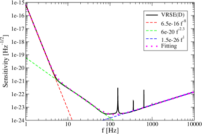
Figure 1: Fitting curve based on the sensitivity curve of KAGRA [bKAGRA, VRSE(D) configuration] shown in Ref. bKAGRA .

To calculate the parameter estimation errors for the inspiral and ringdown GWs, we use the Fisher information matrix,

$$\Gamma_{ij}=\left<\frac{\partial h}{\partial\theta^{i}}\left|\frac{\partial h}{\partial\theta^{j}}\right>\right|_{\theta=\theta_{\rm true}}\,,$$ (16)

where $\theta^{i}$ is the parameters of the waveforms and $\theta_{\rm true}$ denotes the true values of the parameters of the source. Then, the rms errors in the estimated parameters and the covariance between two parameters are derived by the inverse matrix $(\Gamma^{-1})^{ij}$ as

$$(\Delta\theta^{i})_{\rm RMS} = \sqrt{(\Gamma^{-1})^{ii}}\,,$$ (17)

$$c_{ij} = \frac{(\Gamma^{-1})^{ij}}{\sqrt{(\Gamma^{-1})^{ii}(\Gamma^{-1})^{jj}}}\,.$$ (18)

Here, we do not sum over $i$ and $j$. $(\Delta\theta^{i})_{\rm RMS}$ scales as $1/{\rm SNR}$.

For the inspiral phase, we calculate the parameter estimation errors for $\{M,\,\eta,\,t_{c},\,\Phi_{c}\}$, Here, we use the total mass instead of the chirp mass for the parametrization of the inspiral signal, simply because the fitting formulas for the remnant mass and spin are written in terms of $M$ and $\eta$. To evaluate the inner product (12), we take the integration range between $10$Hz and $f_{\rm ISCO}$, For the ringdown phase, we discuss the parameter estimation with respect to $\{f_{c},\,Q,\,t_{0},\,\phi_{0}\}$, and the frequency interval for the integration is between $10$ and $2500$Hz.

We should note that in practice the location of the GW source in the sky and the GW polarization angle in a detector frame are also the parameters to describe the GW signals. For example, Ajith and Bose Ajith:2009fz estimated the parameter errors of BBHs in a single detector or a detector network for the case of the complete set of parameters. This direction to discuss more precise parameter estimation is one of our future studies.

III Simple test of GR

According to Ref. LCGT:2011aa , individual SNRs for the inspiral and ringdown phase signals are comparable for a gravitational wave detector, KAGRA. when the total BBH mass ($\sim$ remnant BH mass) is $\sim 60M_{\odot}$. Since there is a difficulty in determining the initial ringdown amplitude due to the ambiguity of the initial time, for simplicity, we set the SNRs for the inspiral and ringdown phases to be equal for the typical case (with $M=60M_{\odot}$ and $\eta=1/4$ for inspiral and $M_{\rm rem}=57.0904M_{\odot}$ and $\alpha_{\rm rem}=0.686710$ for ringdown). The assumption of the same SNR for the inspiral and ringdown phases is just for simplicity, and we can apply the following analysis for general SNR cases. The information of SNRs is imprinted in the Fisher information matrix of each phase. We briefly discuss the effect by setting different SNRs for the inspiral and ringdown phases in Sec. IV.

III.1 Only ringdown

First, using only the ringdown GWs, we propose a simple method to test whether the compact object emitting the ringdown GWs is a BH predicted by GR or not. Figure 2 shows the QNM frequencies for the dominant $(\ell=2,\,m=2)$ least-damped $(n=0)$ mode in the $(f_{R},\,f_{I})$ plane. In GR, the top-left side of the thick black line is prohibited. The boundary thick black line corresponds to the Schwarzschild limit, which is obtained by setting $\alpha_{\rm rem}=0$, i.e.,

$$\frac{|f_{I}|}{f_{R}}\approx 0.236\,,$$ (19)

in Eqs. (8), (10) and (11). In principle, if we obtain the parameters in the forbidden region from GW observations, we can conclude that the compact object is not the one predicted by GR.

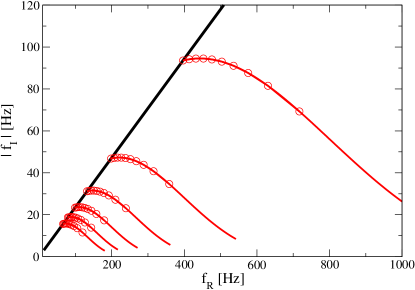
Figure 2: Real ($f_{R}$) and imaginary ($f_{I}$) parts of QNM frequencies for the dominant $(\ell=2,\,m=2)$ least-damped $(n=0)$ mode. The (black) thick line shows the Schwarzschild limit, and the (red) curves are for various mass cases terminated at the spin $\alpha=0.998$ Thorne:1974ve . From the top of the (red) curves, we are considering BH masses, $M/M_{\odot}=30,\,60,\,90,\,120,\,150$, and $180$, respectively. The (red) circles for each line denote the spin dependence $\alpha=0,\,0.1,\,0.2,\,0.3,\,0.4,\,0.5,\,0.6,\,0.7,\,0.8$, and $0.9$ from the left.

However, in practice, there are parameter estimation errors in the GW data analysis. For our typical example with $f_{c}=299.5{\rm Hz},\,Q=3.232,\,t_{0}=0$, and $\phi_{0}=0$ [$f_{R}=299.5{\rm Hz}$ and $f_{I}=-46.34{\rm Hz}$ from Eqs. (8)], we show the contours of the parameter estimation errors in Fig. 3. Here, since we do not discuss the errors of $t_{0}$ and $\phi_{0}$, we integrated the probability distribution over both $t_{0}$ and $\phi_{0}$ Finn:1992wt . In our typical case, the expected errors are sufficiently small to fit the ringdown GW with ${\rm SNR}=50$ within the QNM parameter region allowed in GR at the $5\sigma$ level. On the other hand, the error circle for the signal with ${\rm SNR}=20$ is not sufficiently small in this sense at that level, while it is small enough for 3$\sigma$ level arguments. Here, $5\sigma$ ($3\sigma$) denotes that for the bidimensional (Rayleigh) distribution, which means that the probability falling in the $5\sigma$ ($3\sigma$) circle is about $1-3.7\times 10^{-6}$ ($1-1.1\times 10^{-2}$) since the distribution has 2 degrees of freedom. [In the case of the ordinary one-dimensional Gaussian distribution, the probability falling in the $5\sigma$ ($3\sigma$) region is about $1-5.7\times 10^{-7}$ ($1-2.7\times 10^{-3}$).]

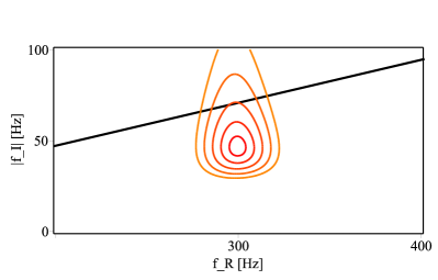
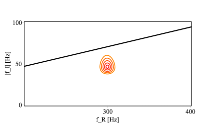
Figure 3: In the ($f_{R},\,f_{I}$) plane, the left and right panels show the parameter estimation in the cases with ${\rm SNR}=20$ and $50$ for the typical case (with $M_{\rm rem}=57.0904M_{\odot}$ and $\alpha_{\rm rem}=0.686710$), respectively. The (black) thick line shows the Schwarzschild limit which is same as that in Fig. 2, and the ellipses are the contours of $1\sigma,\,2\sigma,\,3\sigma,\,4\sigma,$ and $5\sigma$. Here, the time and phase parameters ($t_{0},\,\phi_{0}$) have been marginalized out.

To discuss the region prohibited by GR, we present the parameter estimation for the Schwarzschild ($\alpha_{\rm rem}=0$) case in Fig. 4. Here, we fixed ${\rm SNR}=50$ and considered the remnant masses, $M_{\rm rem}/M_{\odot}=45$, $60$, and $90$. From the $5\sigma$ contours, there is an upper bound of the GR prediction for $|f_{I}|/f_{R}$, and we find that the region of $|f_{I}|/f_{R}>F_{\rm max}$ for each mass case is rejected by GR. Here, $F_{\rm max}$, which denotes the maximum of $|f_{I}|/f_{R}$ allowed in GR, is $0.321$ (for $M_{\rm rem}=45M_{\odot}$), $0.320$ ($60M_{\odot}$) and $0.316$ ($90M_{\odot}$) for ${\rm SNR}=50$. If NR simulations for the extreme spinning BBH are available, we can also give the lower bound of the GR prediction for $|f_{I}|/f_{R}$.

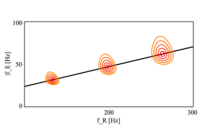
Figure 4: In the ($f_{R},\,f_{I}$) plane, this figure shows the parameter estimation in the cases with ${\rm SNR}=50$ for a Schwarzschild black hole with $M_{\rm rem}/M_{\odot}=45$ (right), $60$ (center) and $90$ (left). The (black) thick line shows the Schwarzschild limit which is same as that in Fig. 2, and the ellipses are the contours of $1\sigma,\,2\sigma,\,3\sigma,\,4\sigma,$ and $5\sigma$. Here, the time and phase parameters ($t_{0},\,\phi_{0}$) have been marginalized out.

It is noted that a powerful method to find ringdown signals in multiple GW detectors has been proposed by Talukder, Bose, Caudill and Baker Talukder:2013ioa . Although we have considered the above GW data analysis with a single detector, we may expect a better parameter estimation in a detector network.

III.2 Consistency analysis with inspiral and ringdown

Next, we propose a consistency test by combining the data from inspiral and ringdown GWs. We use the PN waveform for the inspiral phase to extract the binary parameters, and the formulas in Eqs. (3) and (4) of Sec. II are applied to obtain the GR prediction for the parameters of the remnant black hole. Then, we can present the QNM frequency expected in GR in the ($f_{R},\,f_{I}$) parameter space.

To take into account the observational errors in the estimate of the expected QNM, we assume that the true signal is given by the GR template with $\bm{\theta}$, and the parameters estimated from the inspiral and ringdown signals are $\bm{\theta}_{\rm Insp}$ and $\bm{\theta}_{\rm Ring}$, respectively. Here, $\bm{\theta}$ consists of the parameters $\{f_{c},\,Q,\,t_{0},\,\phi_{0}\}$, which are commonly used for the ringdown GW data analysis. For the ringdown phase, we treat the above parameters to calculate the parameter estimation errors and assume the Gaussian distribution for the parameters. In the inspiral-phase analysis, we use another set of parameters $\tilde{\bm{\theta}}=\{M,\,\eta,\,t_{c},\,\Phi_{c}\}$.

Here, it is useful to have the relation between the inspiral parameters $\tilde{\bm{\theta}}$ and the ringdown parameters $\bm{\theta}$ as fitting functions. From Eq. (4), we have

$$\alpha_{\rm rem} = 0.830028\left(\frac{\eta}{0.25}\right)-0.143761\left(\frac{\eta}{0.25}\right)^{2}+0.00180831\left(\frac{\eta}{0.25}\right)^{12}\,.$$ (20)

The above relation gives one-to-one mapping in the parameter ranges, $0\leq\eta\leq 0.35282872$ and $0\leq\alpha_{\rm rem}\leq 0.99800367$. It is noted that, although $\eta>0.25$ is an unphysical value, we allow the values here. Combining the above equation with Eq. (11), we find that $\eta$ is fitted as a function of $Q$ to obtain

$$\eta = 0.353039-\frac{0.208266}{Q^{2}}-\frac{10.9583}{Q^{4}}-\frac{21.4540}{Q^{6}}\,.$$ (21)

The restriction on the parameter space to keep the one-to-one mapping becomes $2.11870\leq Q\leq 32.2555$. The decay time is calculated as $Q/(\pi f_{c})$. Using Eqs. (3) and (10) (and also the above fitting functions for $\alpha_{\rm rem}$ and $\eta$), the total mass $M$ in the inspiral phase is written by $f_{c}$ and $Q$ as

$$M = \frac{1}{f_{c}}\left[-0.0434932-0.127430\ln\left(\frac{1}{Q}+0.163772\right)+\frac{0.0646167}{\sqrt{Q}}\right]\,.$$ (22)

To find the expected parameter region of the QNM, we use the following simple estimator (more detailed studies, e.g., by using Markov chain Monte Carlo methods, will be presented in future):

$$F(\bm{\theta})={\cal N}\exp\left[-\frac{1}{2}\tilde{\Gamma}_{ij}^{\rm Insp}(\tilde{\theta}^{i}(\bm{\theta})-\tilde{\theta}^{i}(\bm{\theta}_{\rm Insp}))(\tilde{\theta}^{j}(\bm{\theta})-\tilde{\theta}^{j}(\bm{\theta}_{\rm Insp}))-\frac{1}{2}\Gamma_{ij}^{\rm Ring}(\theta^{i}-\theta_{\rm Ring}^{i})(\theta^{j}-\theta_{\rm Ring}^{j})\right]\,,$$ (23)

where ${\cal N}$ is a normalization constant which we do not take care of, and $\tilde{\Gamma}_{ij}^{\rm Insp}$ and $\Gamma_{ij}^{\rm Ring}$ denote the respective Fisher information matrices after integrating the probability distribution over $(t_{c},\,\Phi_{c})$ and $(t_{0},\,\phi_{0})$.

The strategy to estimate the parameter region by using Eq. (23) is as follows:

• For given $\tilde{\bm{\theta}}(\bm{\theta}_{\rm Insp})(=:\tilde{\bm{\theta}}_{\rm Insp})$ (in practice, we give $\tilde{\bm{\theta}}_{\rm Insp}=\{M=60M_{\odot},\,\eta=1/4\}$ and derive $\bm{\theta}_{\rm Insp}$), we calculate $\tilde{\Gamma}_{ij}^{\rm Insp}$ with the bKAGRA noise curve.

• Assuming the narrow ringdown signal in the frequency domain, we prepare $\Gamma_{ij}^{\rm Ring}$ for the white noise (analytically).

• For given $\bm{\theta}_{\rm Ring}$ (and $\Gamma_{ij}^{\rm Ring}$ for it), we find the maximum of Eq. (23) by

  $$\frac{\partial F(\bm{\theta})}{\partial\theta^{i}}=0\,.$$ (24)

• Inserting the solution of the above equation $\bm{\theta}=\{f_{c},\,Q\}$ back into Eq. (23), we check whether the situation with the parameters $(\bm{\theta}_{\rm Insp},\,\bm{\theta}_{\rm Ring},\,\bm{\theta})$ is in the $5\sigma$ level of the detector noise realization or not.

Here, $5\sigma$ denotes that the value in the exponent in Eq. (23) becomes $-5^{2}/2$, which means that the probability falling in the $5\sigma$ circle is about $1-5\times 10^{-5}$ since the distribution has 4 degrees of freedom. Employing our fiducial values, $M=60M_{\odot}$, $\eta=1/4$, the expected region of the QNM frequency in the $5\sigma$ level is shown in Fig. 5. Here, we have fixed ${\rm SNR}=50$ for both the inspiral and ringdown GWs. Compared with the right figure of Fig. 3, the allowed region in this figure has a larger extension in the horizontal direction. This is due to the parameter estimation errors of the inspiral phase. We repeat the meaning of this plot. Under the condition that we measure the values of both $\tilde{\bm{\theta}}_{\rm Insp}$ and $\bm{\theta}_{\rm Ring}$, we choose the most probable values for the parameters $\bm{\theta}$. Assuming that the true values are the most probable values as used in the usual Fisher-matrix analysis, we evaluate the probability that the detector noise produces such a deviation in the measurement of $\tilde{\bm{\theta}}_{\rm Insp}$ and $\bm{\theta}_{\rm Ring}$. The probability that the noise realization falls outside the contour is $5\times 10^{-5}$. Therefore, if we find that the parameter estimate from the ringdown signal deviates from the prediction from the inspiral signal exceeding the contour in Fig. 3, we can conclude that there is something wrong with the GR prediction. Here, under an assumption that the nonlinearity of GR is correct for the inspiral and merger phases, it is possible to distinguish the remnant object from the BHs that are predicted by GR.

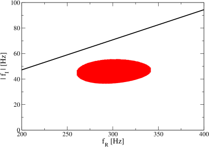
Figure 5: The QNM frequency expected in GR ($5\sigma$ level) from the inspiral phase with the total mass $M=60M_{\odot}$ and symmetric mass ratio $\eta=1/4$ [the (red) filled region]. The (black) thick line shows the Schwarzschild limit which is same as that in Fig. 2.

IV Summary and Discussion

In this paper, we mainly focused on a specific BBH with the total mass $M=60M_{\odot}$ and the symmetric mass ratio $\eta=1/4$, which would be the typical one for Pop III BBHs Kinugawa:2014zha ; Kinugawa:2015 . It is found that we can perform meaningful tests of GR, assuming that the GW signal has ${\rm SNR}=50$. An easy extension of the present study is to treat various total mass cases. For total masses lower than $M=60M_{\odot}$, we have fewer SNRs for the ringdown phase than those for the inspiral phase and expect that a larger elongation in the vertical direction in the $(f_{R},\,f_{I})$ plane because of Fig. 3. On the other hand, for total masses higher than $M=60M_{\odot}$, we will have a larger elongation in the horizontal direction. We also need to discuss various mass ratios and spins in the inspiral phase. The statistical treatment will be also improved in our future work.

In Fig. 5, we have observed that the expected region shows a large elongation in the horizontal direction. This is due to the parameter estimation errors for the inspiral signal and, more specifically, originates from marginalizing $t_{c}$ and $\Phi_{c}$ in the probability distribution. The parameter estimation errors of $t_{c}$ and $\Phi_{c}$ arise from the short frequency integration interval between $10$Hz and $f_{\rm ISCO}=73.28$Hz . The number of GW cycles during this frequency range is $N_{\rm GW}\approx 30$. When we change the lower integration bound to $20$Hz, the situation becomes much worse, i.e., the number of GW cycles is just $N_{\rm GW}\approx 6$.

Here, if we can also detect the inspiral phase by using a space-based GW detector, such as DECIGO Seto:2001qf , the situation will improve a lot (see, e.g., Ref. Nair:2015bga for the synergy in the parameter estimation of binary inspirals). For example, $N_{\rm GW}\approx 5400$ from $0.5$Hz in our specific case. Therefore, even if we assume the same SNR for the inspiral phase, the parameter estimation of $M$ and $\eta$ and the QNM prediction will be very precise.

Kinugawa et al. Kinugawa:2015 showed that the expected detection rate of BH-BH mergers by KAGRA with typical total mass $\sim 60M_{\odot}$ is given by

$$262\,{\rm events~{}yr^{-1}(SFR_{P}/(10^{-2.5}~{}M_{\odot}\rm~{}yr^{-1}~{}Mpc^{-3}))\cdot Err_{sys}}\,,$$ (25)

where $\rm SFR_{p}$ and $\rm Err_{sys}$ are the peak value of the Pop III star formation rate and the systematic error with $\rm Err_{sys}=1$ for their fiducial model, respectively. They have estimated that ${\rm Err_{sys}}$ ranges from 0.056 to 2.3 due to the unknown parameters such as the common envelope parameter, the kick velocity, and the loss fraction as well as the unknown distribution functions such as the initial mass function and the initial eccentricity function. The minimum value corresponds to the worst model in which they adopt the most pessimistic values of the parameters and distribution functions within the ranges that are likely. The factor ${\rm(SFR_{P}/(10^{-2.5}~{}M_{\odot}\rm~{}yr^{-1}~{}Mpc^{-3}))}$ also depends on the models and Kinugawa et al. Kinugawa:2015 argued that it ranges from 0.019 to 16. Therefore, the event rate of Pop III BH-BH mergers which will be detected by KAGRA ranges from 0.28 to 9641 ${\rm yr^{-1}}$. The event rate for Advanced LIGO and Advanced Virgo will be similar. Since no such event has been found so far, the event rate should be smaller than 1000 ${\rm yr^{-1}}$. Adopting a simple geometric mean of this allowed range, we have a rough estimate of the expected rate of 500 ${\rm yr^{-1}}$. Then, the rates of events with ${\rm SNR}>20$ and ${\rm SNR}>50$ are 32 and 2 ${\rm yr^{-1}}$, respectively. Therefore, there is a good chance to confirm (or refute) the Einstein theory in the strong gravity regime by observing the expected QNMs.

- (1) P. O. Mazur and E. Mottola, gr-qc/0109035.
- (2) S. D. Mathur, Fortsch. Phys. 53, 793 (2005) [hep-th/0502050].
- (3) S. L. Braunstein, S. Pirandola, and K, Życzkowski, Phys. Rev. Lett. 110, 101301 (2013) [arXiv:0907.1190 [quant-ph]].
- (4) A. Almheiri, D. Marolf, J. Polchinski, and J. Sully, JHEP 1302, 062 (2013) [arXiv:1207.3123 [hep-th]].
- (5) L. Modesto, Phys. Rev. D 86, 044005 (2012) [arXiv:1107.2403 [hep-th]].
- (6) T. Biswas, E. Gerwick, T. Koivisto, and A. Mazumdar, Phys. Rev. Lett. 108, 031101 (2012) [arXiv:1110.5249 [gr-qc]].
- (7) E. Berti et al., arXiv:1501.07274 [gr-qc].
- (8) O. Dreyer, B. J. Kelly, B. Krishnan, L. S. Finn, D. Garrison, and R. Lopez-Aleman, Class. Quant. Grav. 21, 787 (2004) [gr-qc/0309007].
- (9) E. Berti, V. Cardoso, and A. O. Starinets, Class. Quant. Grav. 26, 163001 (2009) [arXiv:0905.2975 [gr-qc]].
- (10) S. A. Hughes and K. Menou, Astrophys. J. 623, 689 (2005) [astro-ph/0410148].
- (11) S. W. Hawking, Phys. Rev. Lett. 26, 1344 (1971).
- (12) L. Blanchet, Living Rev. Rel. 17, 2 (2014) [arXiv:1310.1528 [gr-qc]].
- (13) G. Schaefer, Fundam. Theor. Phys. 162, 167 (2011) [arXiv:0910.2857 [gr-qc]].
- (14) F. Pretorius, Phys. Rev. Lett. 95, 121101 (2005) [gr-qc/0507014].
- (15) M. Campanelli, C. O. Lousto, P. Marronetti, and Y. Zlochower, Phys. Rev. Lett. 96, 111101 (2006) [gr-qc/0511048].
- (16) J. G. Baker, J. Centrella, D. I. Choi, M. Koppitz, and J. van Meter, Phys. Rev. Lett. 96, 111102 (2006) [gr-qc/0511103].
- (17) M. Luna and A. M. Sintes, Class. Quant. Grav. 23, 3763 (2006) [gr-qc/0601072].
- (18) T. Kinugawa, K. Inayoshi, K. Hotokezaka, D. Nakauchi, and T. Nakamura, Mon. Not. Roy. Astron. Soc. 442, 2963 (2014) [arXiv:1402.6672 [astro-ph.HE]].
- (19) T. Kinugawa, A. Miyamoto, N. Kanda, and T. Nakamura, [arXiv:1505.06962 [astro-ph.SR]].
- (20) T. Damour, B. R. Iyer, and B. S. Sathyaprakash, Phys. Rev. D 63, 044023 (2001) [Erratum-ibid. D 72, 029902 (2005)] [gr-qc/0010009].
- (21) P. Ajith, M. Boyle, D. A. Brown, S. Fairhurst, M. Hannam, I. Hinder, S. Husa, B. Krishnan, R. A. Mercer, F. Ohme, C. D. Ott, J. S. Read, L. Santamaria, and J. T. Whelan, arXiv:0709.0093 [gr-qc].
- (22) C. Cutler and E. E. Flanagan, Phys. Rev. D 49, 2658 (1994) [gr-qc/9402014].
- (23) A. Taracchini et al., Phys. Rev. D 89, 061502 (2014) [arXiv:1311.2544 [gr-qc]].
- (24) J. Healy, C. O. Lousto, and Y. Zlochower, Phys. Rev. D 90, 104004 (2014) [arXiv:1406.7295 [gr-qc]].
- (25) A. Ori and K. S. Thorne, Phys. Rev. D 62, 124022 (2000) [gr-qc/0003032].
- (26) H. Nakano, Class. Quant. Grav. 32, 177002 (2015) [arXiv:1501.02890 [gr-qc]].
- (27) H. Nakano, J. Healy, C. O. Lousto, and Y. Zlochower, Phys. Rev. D 91, 104022 (2015) [arXiv:1503.00718 [gr-qc]].
- (28) E. Berti, V. Cardoso, and C. M. Will, Phys. Rev. D 73, 064030 (2006) [gr-qc/0512160].
- (29) http://www.phy.olemiss.edu/~berti/qnms.html
- (30) K. Somiya (KAGRA Collaboration), Class. Quant. Grav. 29, 124007 (2012) [arXiv:1111.7185 [gr-qc]].
- (31) Y. Aso et al. (KAGRA Collaboration), Phys. Rev. D 88, 043007 (2013) [arXiv:1306.6747 [gr-qc]].
- (32) http://gwcenter.icrr.u-tokyo.ac.jp/researcher/parameters
- (33) J. Aasi et al. (LIGO Scientific Collaboration), Class. Quant. Grav. 32, 074001 (2015) [arXiv:1411.4547 [gr-qc]].
- (34) F. Acernese et al. (VIRGO Collaboration), Class. Quant. Grav. 32, 024001 (2015) [arXiv:1408.3978 [gr-qc]].
- (35) C. Affeldt et al., Class. Quant. Grav. 31, 224002 (2014).
- (36) P. Ajith and S. Bose, Phys. Rev. D 79, 084032 (2009) [arXiv:0901.4936 [gr-qc]].
- (37) N. Kanda (LCGT Collaboration), arXiv:1112.3092 [astro-ph.IM].
- (38) K. S. Thorne, Astrophys. J. 191, 507 (1974).
- (39) L. S. Finn, Phys. Rev. D 46, 5236 (1992) [gr-qc/9209010].
- (40) D. Talukder, S. Bose, S. Caudill, and P. T. Baker, Phys. Rev. D 88, 122002 (2013) [arXiv:1310.2341 [gr-qc]].
- (41) N. Seto, S. Kawamura, and T. Nakamura, Phys. Rev. Lett. 87, 221103 (2001) [astro-ph/0108011].
- (42) R. Nair, S. Jhingan, and T. Tanaka, arXiv:1504.04108 [gr-qc].