Risks aggregation in multivariate dependent Pareto distributions

José María Sarabia^a, Emilio Gómez-Déniz^b
Faustino Prieto^a, Vanesa Jordá^a

^aDepartment of Economics, University of Cantabria, Avda de los Castros s/n, 39005-Santander, Spain

^bDepartment of Quantitative Methods in Economics and TiDES Institute, University of Las Palmas de Gran Canaria, 35017-Las Palmas de G.C., Spain

Abstract

In this paper we obtain closed expressions for the probability distribution function, when we consider aggregated risks with multivariate dependent Pareto distributions. We work with the dependent multivariate Pareto type II proposed by Arnold (1983, 2015), which is widely used in insurance and risk analysis. We begin with the individual risk model, where we obtain the probability density function (PDF), which corresponds to a second kind beta distribution. We obtain several risk measures including the VaR, TVaR and other tail measures. Then, we consider collective risk model based on dependence, where several general properties are studied. We study in detail some relevant collective models with Poisson, negative binomial and logarithmic distributions as primary distributions. In the collective Pareto-Poisson model, the PDF is a function of the Kummer confluent hypergeometric function, and in the Pareto-negative binomial is a function of the Gauss hypergeometric function. Using the data set based on one-year vehicle insurance policies taken out in 2004-2005 (Jong and Heller, 2008), we conclude that our collective dependent models outperform the classical collective models Poisson-exponential and geometric-exponential in terms of the AIC and CAIC statistics.

Key Words: Dependent risks; individual risk model; collective risk model.

1 Introduction

In the context of the classical theory of risk, consider the individual and the collective risk models (see Kass et al. (2001) and Klugman et al. (2008)). These models rely on the assumptions of the independence between: (i) different claim amounts; (ii) the number of claims and claim amounts and (iii) claim amounts and interclaim times.

The use of the independence hypothesis facilitates the computation of many risks measures, but can be restrictive in different contexts. The need for generalizations in both individual and collective classical models (by considering some kind of dependence structure) has led several researches to model dependence.

In this context, Sarabia and Guillén (2008) have considered extensions of the classical collective model assuming that the conditional distributions $S|N$ and $N|S$ belong to some prescribed parametric family, where $S$ is the total claim amount and $N$ is the number of claims. Gómez-Déniz and Calderín-Ojeda (2014), using conditional specification techniques, have obtained discrete distributions to be used in the collective risk model to compute the right-tail probability of the aggregate claims size distribution.

Albrecher and Teugels (2006) have considered a dependence structure based on a copula for the interclaim time and the subsequent claim size. Boudreault et al. (2006) studied an extension of the classical compound Poisson risk model, where the distribution of the next claim amount was defined as a function of the time elapsed since the last claim. Cossette et al. (2008) have considered another extension introducing a dependence structure between the claim amounts and the interclaim time using a generalized Farlie-Gumbel-Morgenstern copula. Cossette et al. (2004) have considered a variation of the compound binomial model in a markovian environment, which is an extension of the model presented by Gerber (1998). Compound Poisson approximations for individual models with dependent risk was considered by Genest et al (2003).

A recent model of dependence between risks has been proposed by Cossette et al. (2013). These authors consider a portfolio of dependent risks whose multivariate distribution is defined with the Farlie-Gumbel-Morgenstern copula, with mixed Erlang distribution marginals.

In this paper we obtain closed expressions for the probability distribution function modeling aggregated risks with multivariate dependent Pareto distributions between the different claim amounts. We work with the dependent multivariate Pareto type II proposed by Arnold (1983, 2015), which is widely used in insurance and risk analysis. We begin with the classical individual risk model. For this model we obtain the probability density function (PDF), which corresponds to a second kind beta distribution. We also obtain several risk measures including the VaR, TVaR and other tail measures. Then, we consider collective risk model based on dependence, whose main general properties are studied. We study in detail some relevant collective models with Poisson, negative binomial and logarithmic distributions as primary distributions. For these three models, we obtain simple and closed expressions for the aggregated distributions.

The contents of this paper are the following. In Section 2 we present the main univariate distributions used in the paper. The class of multivariate dependent Pareto distribution considered to model aggregated risks is presented in 3. Section 4 presents the individual risk model under dependence and Section 5 introduces the collective risk model under dependence. After presenting general results we study the compound models where the primary distribution is Poisson, negative binomial, geometric and logarithmic and the secondary distribution is Pareto. Section 6 includes an example with real data. The conclusions of the paper are given in Section 7.

2 Univariate distributions

In this section, we introduce several univariate random variables which will be used in the paper.

We work with the Pareto distribution with PDF given by,

$$f(x;\alpha,\beta)=\frac{\alpha}{\beta(1+x/\beta)^{\alpha+1}},\;\;x>0,$$ (1)

and $f(x;\alpha,\beta)=0$ if $x<0$, where $\alpha,\beta>0$. Here, $\alpha$ is a shape parameter and $\beta$ is a scale parameter. We represent $X\sim{\cal P}a(\alpha,\beta)$.

We denote by $X\sim{\cal G}a(\alpha)$ a gamma random variable with PDF $f(x)=\frac{x^{\alpha-1}e^{-x}}{\Gamma(\alpha)}$ if $x>0$, whith $\alpha>0$. The exponential distribution with mathematical expectation 1 is denoted by ${\cal G}a(1)$.

The following lemma provides a simple stochastic representation of the Pareto distribution as quotient of random variables. The proof is straightforward and will be omitted.

Lemma 1

Let $U_{1}$ and $U_{\alpha}$ independent gamma random variables such that $U_{1}\sim{\cal G}a(1)$ and $U_{\alpha}\sim{\cal G}a(\alpha)$, where $\alpha>0$. If $\beta>0$, the random variable,

$$X=\beta\frac{U_{1}}{U_{\alpha}}\sim{\cal P}a(\alpha,\beta).$$ (2)

An extension of the Pareto distribution (1) is the following. A random variable $X$ is said to be a second kind beta distribution if its PDF is of the form,

$$f(x;p,q,\beta)=\frac{x^{p-1}}{\beta^{p}B(p,q)(1+x/\beta)^{p+q}},\;\;x>0,$$ (3)

and $f(x;p,q,\beta)=0$ if $x<0$, where $p,q,\beta>0$ and $B(p,q)=\frac{\Gamma(p)\Gamma(q)}{\Gamma(p+q)}$ denotes the beta function. This random variable corresponds to the Pearson VI distribution in the classical Pearson systems of distributions and we represent $X\sim{\cal B}2(p,q,\lambda)$. If we set $p=1$ in (3), we obtain a Pareto distribution ${\cal P}a(q,\beta)$ like (1).

The second kind beta distribution has a simple stochastic representation as a ratio of gamma random variables. If $U_{p}$ and $U_{q}$ are independent gamma random variables, the new random variable $X=\beta\frac{U_{p}}{U_{q}}$ has the PDF defined in (3).

3 The multivariate Pareto class

Now we present the class of multivariate dependent Pareto distribution which will be used in the different models.

In the literature several classes of multivariate Pareto distributions have been proposed. One of the main classes was introduced by Arnold (1983, 2015), in the context of the hierarchy Pareto distributions proposed by this author. Other classes were proposed by Chiragiev and Landsman (2009) and Asimit et al. (2010). The conditional dependence structure is the base of the construction of the proposals by Arnold (1987) and Arnold et al. (1993) (see also Arnold et al, 2001), where two different dependent classes are obtained.

Definition 1

Let $Y_{1},Y_{2},\dots,Y_{n}$ and $Y_{\alpha}$ be mutually independent gamma random variables with distributions $Y_{i}\sim{\cal G}a(1)$, $i=1,2,\dots,n$ and $Y_{\alpha}\sim{\cal G}a(\alpha)$ with $\alpha>0$. The multivariate dependent Pareto distribution is defined by the stochastic representation,

$$\bm{X}=\left(X_{1},X_{2},\dots,X_{n}\right)^{\top}=\left(\beta\frac{Y_{1}}{Y_{\alpha}},\beta\frac{Y_{2}}{Y_{\alpha}},\dots,\beta\frac{Y_{n}}{Y_{\alpha}}\right)^{\top},$$ (4)

where $\beta>0$.

Note that the common random variable $Y_{\alpha}$ introduces the dependence in the model.

3.1 Properties of the multivariate Pareto class

We describe several properties of the multivariate Pareto defined in (1).

• Marginal distributions. By construction, the marginal distributions are Pareto,

  $$X_{i}\sim{\cal P}a(\alpha,\beta),\;\;i=1,2,\dots,n.$$

• The joint PDF of the vector $\bm{X}$ is given by,

  $$f(x_{1},\dots,x_{n};\alpha,n)=\frac{\Gamma(\alpha+n)}{\Gamma(\alpha)\beta^{n}}\frac{1}{(1+\sum_{i=1}^{n}x_{i}/\beta)^{\alpha+n}},\;\;x_{1},\dots,x_{n}>0.$$ (5)

  This expression corresponds to the multivariate Pareto type II proposed by Arnold (1983, 2015).

• The covariance matrix is given by,

  $$cov(X_{i},X_{j})=\frac{\beta^{2}}{(\alpha-1)^{2}(\alpha-2)},\;\;\alpha>2,\;\;i\neq j$$

  and the correlation between components is,

  $$\rho(X_{i},X_{j})=\frac{1}{\alpha},\;\;\alpha>2,\;\;i\neq j$$

• General moments. The moments of (1) are,

  $$E[X_{1}^{r_{1}}\cdots X_{n}^{r_{n}}]=\frac{\Gamma(\alpha-A)}{\Gamma(\alpha)}\prod_{i=1}^{n}\beta^{r_{i}}\Gamma(1+r_{i}),$$

  where $A=r_{1}+\dots+r_{m}$ and $\alpha>A$.

The dependence structure of $\bm{X}$ is studied in the following result

Proposition 1

The random variables $\bm{X}=(X_{1},\dots,X_{n})^{\top}$ are associated, and then $\mbox{cov}(X_{i},X_{j})\geq 0$, if $i\neq j$.

Proof:   See Appendix.  

Remark: Let us consider the multivariate Pareto survival function of (5) given by,

$$\bar{F}(x_{1},\dots,x_{n})=\left(1+\sum_{i=1}^{n}\frac{x_{i}}{\beta}\right)^{-\alpha},\;\;x_{1},\dots,x_{n}>0,$$

with $\alpha,\beta>0$. For this family, the associated copula is the Pareto copula or Clayton copula,

$$C(u_{1},\dots,u_{n};\alpha)=\left(u_{1}^{-1/\alpha}+\dots+u_{n}^{-1/\alpha}-n+1\right)^{-\alpha}.$$

Note that the dependence increases with $\alpha$, being the independence case obtained when $\alpha\to 0$ and the Fréchet upper bound when $\alpha\to\infty$ .

4 The individual risk model under Pareto dependence

In this section we consider the individual risk model assuming dependence between risks. The distribution of sums of iid Pareto distributions was obtained by Ramsay (2006). Let $(X_{1},\dots,X_{n})^{\top}$ be the multivariate Pareto distribution defined in (4). Then, we consider the aggregate risks $S_{n}=X_{1}+\dots+X_{n}$. We have the following result.

Theorem 1

The PDF of the aggregate random variable $S_{n}$, where the components are Pareto defined in (1) is given by,

$$f_{S_{n}}(x;n,\alpha,\beta)=\frac{x^{n-1}}{\beta^{n}B(n,\alpha)(1+x/\beta)^{n+\alpha}},\;\;x>0$$

end $f_{S_{n}}(x;n,\alpha,\beta)=0$ if $x<0$, that is $S_{n}\sim{\cal B}2(n,\alpha,\beta)$.

Proof:   See Appendix.  

Note that (1) corresponds to the PDF of a second kind beta distribution defined in (3). Figure 1 represents the PDF (1) for $\alpha=1/2;1;2$ and $10$ for $n=2,5,10$ and $20$.

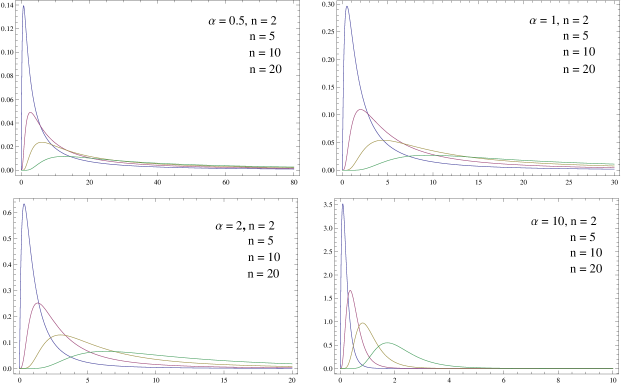
Figure 1: PDF of the individual model $S_{n}$ for some selected values of $\alpha$ and $n$.

4.1 Risk measures

Here we present some risk measures for the second kind beta distribution, which can be applied for the aggregate PDF given in (1). The value at risk VaR at level $u$, with $0<u<1$ of a random variable $X$ with CDF $F(x)$ is defined as,

$$\mbox{VaR}[X;u]=\inf\{x\in\mathbb{R},\,F(x)\geq u\}.$$

If $X\sim{\cal B}2(p,q,\beta)$, Guillén et al. (2013) have obtained that,

$$\mbox{VaR}[X;u]=\beta\frac{IB^{-1}(u;p,q)}{1-IB^{-1}(u;p,q)},$$ (6)

where $IB^{-1}(u;p,q)$ denotes the inverse of the incomplete ratio beta function, which corresponds to the quantile function of the classical beta distribution of the first kind. Then, using (6) for the aggregate distribution (1) we have

$$\mbox{VaR}[S_{n};u]=\beta\frac{IB^{-1}(u;n,\alpha)}{1-IB^{-1}(u;n,\alpha)},$$

with $0<u<1$.

The following result provides higher moments of the worst $x_{u}$ events, which extend popular risk measures.

Lemma 2

Let $X\sim{\cal B}2(p,q,\beta)$ be a second kind beta distribution. Then, the conditional tail moments are given by,

$$E[X^{r}|X>x_{u}]=\frac{\beta^{r}\Gamma(p+r)\Gamma(q-r)}{(1-u)\Gamma(p)\Gamma(q)}\left\{1-B\left(\frac{x_{u}/\beta}{1+x_{u}/\beta};p+r,q-r\right)\right\},$$ (7)

where $x_{u}=VaR[X;u]$ represents the value at risk with $u\in(0,1)$.

Proof:   See Appendix.  

If we take $r=1$ in (7) we obtain the tail value at risk TVaR, which was obtained by Guillén et al. (2013).

5 The collective risk model under dependence

In this section we consider the collective model based on dependence between claim amounts. Let $N$ be the number of claims in a portfolio of policies in a time period. Let $X_{i}$, $i=1,2,\dots$ be the amount of the $i$th claim and $S_{N}=X_{1}+\dots+X_{N}$ the aggregate claims of the portfolio in the time period considered.

5.1 General properties

We consider two assumptions: (1) We assume that all the claims $X_{1},X_{2},\dots,X_{n},\dots$ are dependent random variables with the same distribution and (2) The random variable $N$ is independent of all claims $X_{1},X_{2},\dots,X_{n},\dots$

Theorem 2

Let $(X_{1},X_{2},\dots,X_{n},\dots)$ be dependent random variables with common CDF $F(x)$, and let $N$ be the observed number of claims, with PMF given by $p_{n}=\Pr(N=n)$, for $n=0,1,\dots$, which is independent of all $X_{i}$’s, $i=1,2,\dots$ Then, the CDF of the aggregate losses $S_{N}$ is,

$$F_{S_{N}}(x)=\sum_{n=0}^{\infty}p_{n}F_{X}^{(n)}(x),$$

where $F_{X}^{(n)}(x)$ represent the CDF of the convolution of the $n$ dependent claims $(X_{1},\dots,X_{n})$.

Proof:   See Appendix.  

The mean and the variance of the collective model can be found in the following result.

Lemma 3

The mean and the variance of $S_{N}$ under dependence are given by,

$$E(S_{N}) = E(N)E(X),$$ (8)

$$var(S_{N}) = E(N)var(X)+var(N)(E(X))^{2}+E[N(N-1)]cov(X_{i},X_{j})$$ (9)

Proof:   See Appendix.  

If the claims $X_{i}$ and $X_{j}$ are independent $cov(X_{i},X_{j})=0$ and then (9) becomes in the usual formula for $var(S_{N})$.

On the other hand, if the random variables $\{X_{i}\}$ are associated,

$$\mbox{var}(S_{N}^{(I)})<\mbox{var}(S_{N}^{(D)}),$$

where $\mbox{var}(S_{n}^{(I)})$ is the variance in the independent case and $\mbox{var}(S_{n}^{(D)})$ the variance in the dependent case. This fact is a consequence of the associated property, which leads to a positive variance between $X_{i}$ and $X_{j}$.

5.2 Compound Pareto models

In this section we obtain the distribution of the compound collective model $S_{N}=X_{1}+X_{2}+\dots+X_{N}$ where the secondary distribution is Pareto given by (4), and several primary distribution are considered for $N$.

In the case of independence between claims $X_{i}$ this distribution was studied by Ramsay (2009) when the primary distribution is Poisson and negative binomial cases.

5.2.1 The compound Pareto-Poisson distribution

We consider the model where the primary distribution is a Poisson distribution.

Theorem 3

If we assume a Poisson distribution with parameter $\lambda$ as primary distribution and $(X_{1},\dots,X_{n})$ is defined in (1), the PDF of the random variable $S_{N}$ is given by,

$$f_{S_{N}}(x;\alpha,\lambda,\beta)=\frac{\alpha\lambda e^{-\lambda}}{\beta(1+x/\beta)^{\alpha+1}}{}_{1}F_{1}\left[1+\alpha;2;\frac{\lambda x/\beta}{1+x/\beta}\right],\;\;x>0$$ (10)

and $f_{S_{N}}(0;\alpha,\lambda,\beta)=e^{-\lambda}$ where ${}_{1}F_{1}(a;b;z)$ denotes the Kummer confluent hypergeometric function defined by,

$${}_{1}F_{1}[a;b;z]=\sum_{n=0}^{\infty}\frac{(a)_{n}z^{n}}{(b)_{n}n!},$$

where $(a)_{n}$ represent the Pochhammer symbol defined by $(a)_{n}=a(a-1)\dots(a-n+1)$.

Proof:   See Appendix.  

Figure 2 represents the PDF (10) Pareto-Poisson for some values of $\alpha=0,5;1;2$ and 10 and $\lambda=2,5,10$ and 20, taking $\beta=1$.

Figure 2: PDF of the collective model Pareto-Poisson for $\beta=1$ and selected values of $\alpha$ and $\lambda$.

Using formulas (8) and (9), the mean and variance of the dependent Pareto-Poisson collective model are given by,

$$E(S_{N}) = \frac{\lambda\beta}{\alpha-1},\;\;\alpha>1,$$

$$var(S_{N}) = \frac{\alpha\beta^{2}(\lambda+2\alpha-2)}{(\alpha-1)^{2}(\alpha-2)},\;\;\alpha>2.$$

5.2.2 The compound Pareto-negative binomial distribution

Let $N$ be a negative binomial distribution with PMF,

$$\Pr(N=n)=\frac{\Gamma(n+r)}{\Gamma(n+1)\Gamma(r)}p^{r}(1-p)^{n},\;\;n=0,1,2,\dots$$ (11)

We have the following theorem.

Theorem 4

If we assume a negative binomial distribution with parameter $r$ and $p$ and PMF given by (11) as primary distribution and $(X_{1},\dots,X_{n})$ is defined in (4), the PDF of the random variable $S_{N}$ is given by,

$$f_{S_{N}}(x;\alpha,\beta,r,p)=\frac{r\alpha(1-p)p^{r}}{\beta(1+x/\beta)^{\alpha+1}}{}_{2}F_{1}\left[1+r,1+\alpha;2;\frac{(1-p)x/\beta}{1+x/\beta}\right],\;\;x>0$$

and $f_{S_{N}}(0;\alpha,\beta,r,p)=p^{r}$, where ${}_{2}F_{1}(a,b;c;z)$ denotes the Gauss hypergeometric function defined by,

$${}_{2}F_{1}[a,b;c;z]=\sum_{n=0}^{\infty}\frac{(a)_{n}(b)_{n}z^{n}}{(c)_{n}n!},$$

where $(a)_{n}$ denotes the Pochhammer symbol.

The proof is similar to the proof in Theorem 3 and will be omitted.

Again, using formulas (8) and (9), the mean and variance of the dependent Pareto-negative binomial collective model are given by,

$$E(S_{N}) = \frac{r(1-p)\beta}{p(\alpha-1)},\;\;\alpha>1,$$

$$var(S_{N}) = \frac{r(1-p)\beta^{2}((1+p)(\alpha-1)+r(1-p))}{p^{2}(\alpha-1)^{2}(\alpha-2)},\;\;\alpha>2.$$

5.2.3 The compound Pareto-geometric distribution

In this result we obtain the PDF of the Pareto-geometric distribution.

Corollary 1

If we assume a geometric distribution with parameter and PMF given by $\Pr(N=n)=p(1-p)^{n}$, $n=0,1,\dots$ as primary distribution and $(X_{1},\dots,X_{n})$ is defined in (4), the PDF of the random variable $S_{N}$ is given by,

$$f_{S_{N}}(x;\alpha,\beta,p)=\frac{\alpha p(1-p)}{\beta(1+px/\beta)^{\alpha+1}},\;\;x>0$$ (12)

and $f_{S_{N}}(0;\alpha,\beta,p)=p$.

Figure 3 represents the PDF (12) for some selected values of $\alpha$ and $p$ ($\beta=1$).

Figure 3: PDF of the collective model Pareto-Geometric for $\beta=1$ and selected values of $\alpha$ and $p$.

5.2.4 The compound Pareto-logarithmic distribution

Let $N$ be a discrete logarithmic distribution with PMF,

$$\Pr(N=n)=-\frac{1}{\log(1-\theta)}\frac{\theta^{n}}{n},\;\;n=1,2,\dots,$$ (13)

where $\theta\in(0,1)$.

We have the following theorem.

Theorem 5

If we assume a logarithmic distribution with parameter $\theta$ and PMF given by (13) as primary distribution and $(X_{1},\dots,X_{n})$ is defined in (1), the PDF of the random variable $S_{N}$ is given by,

$$f_{S_{N}}(x;\alpha,\beta,\theta)=-\frac{1}{\log(1-\theta)}\left[\frac{1}{x(1+(1-\theta)x/\beta)^{\alpha}}-\frac{1}{x(1+x/\beta)^{\alpha}}\right],\;\;x>0$$ (14)

and $f_{S_{N}}(x;\alpha,\beta,\theta)=0$, if $x<0$.

The proof of this result is omitted.

Figure 4 represents the PDF (14) Pareto-Logarithmic for some values of $\alpha=0,5;1;2$ and 10 and $\theta=0.2;0.4;0.6$ and $0.8$ taking $\beta=1$.

The mean and variance of the dependent Pareto-Logarithmic collective model are

$$E(S_{N}) = \frac{a\beta\theta}{(\alpha-1)(1-\theta)},\;\;\alpha>1,$$

$$var(S_{N}) = \frac{a\beta^{2}\theta(2(\alpha-1)-\alpha\theta(1+a)+\theta(1+2a)}{(\alpha-1)^{2}(\alpha-2)(1-\theta)^{2}},\;\;\alpha>2,$$

being $a=-1/\log(1-\theta)$.

Figure 4: PDF of the collective model Pareto-Logarithmic for $\beta=1$ and selected values of $\alpha$ and $\theta$.

6 A Numerical application with real data

In order to compare the performance of the models presented in this paper, we examined a data set based on one-year vehicle insurance policies taken out in 2004 or 2005. This data set is available on the website of the Faculty of Business and Economics, Macquarie University (Sydney, Australia) (see also Jong and Heller (2008)). The first 100 observations of this data set are shown in Table 1, with the following elements: from left to right, the policy number, the number of claims and the size of the claims. The total portfolio contains 67856 policies of which 4624 have at least one claim. Some descriptive statistics for this data set are shown in Table 2. It can be seen that the standard deviation is very large for the size of the claims, which means that a premium based only on the mean size of the claims is not adequate for computing the bonus-malus premiums. The covariance between the claims and sizes is positive and takes the value 141.574.

Table 1: First 100 observations of the data set

1	0	0	21	0	0	41	2	1811.71	61	0	0	81	0	0
2	0	0	22	0	0	42	0	0	62	0	0	82	0	0
3	0	0	23	0	0	43	0	0	63	0	0	83	0	0
4	0	0	24	0	0	44	0	0	64	0	0	84	0	0
5	0	0	25	0	0	45	0	0	65	1	5434.44	85	0	0
6	0	0	26	0	0	46	0	0	66	1	865.79	86	0	0
7	0	0	27	0	0	47	0	0	67	0	0	87	0	0
8	0	0	28	0	0	48	0	0	68	0	0	88	0	0
9	0	0	29	0	0	49	0	0	69	0	0	89	0	0
10	0	0	30	0	0	50	0	0	70	0	0	90	0	0
11	0	0	31	0	0	51	0	0	71	0	0	91	0	0
12	0	0	32	0	0	52	0	0	72	0	0	92	0	0
13	0	0	33	0	0	53	0	0	73	0	0	93	0	0
14	0	0	34	0	0	54	0	0	74	0	0	94	0	0
15	1	669.51	35	0	0	55	0	0	75	0	0	95	0	0
16	0	0	36	0	0	56	0	0	76	0	0	96	1	1105.77
17	1	806.61	37	0	0	57	0	0	77	0	0	97	0	0
18	1	401.80	38	0	0	58	0	0	78	0	0	98	0	0
19	0	0	39	0	0	59	0	0	79	0	0	99	1	200
20	0	0	40	0	0	60	0	0	80	0	0	100	0	0

Figure 6 shows the complete number of claims and the total claim amount concerning these claims. It can be seen that the largest claim values appear in the case of single claims, while these values fall with larger numbers of claims.

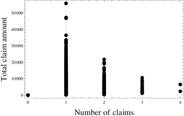
Figure 5: Number of claims and their sizes

Table 2: Some descriptive data of claims and claim size for the data set

	Number of claims	Total claim amount
Mean	0.072	137.27
Standard deviation	0.278	1056.30
$\min$	0	0
$\max$	4	55922.10

In this regard, the compound Poisson model has been traditionally considered when the size of a single claim is modeled by an exponential distribution, chiefly because of the complexity of the collective risk model under other probability distributions such as Pareto and log-normal distributions.

Perhaps the most well-known aggregate claims model is the obtained when the primary and secondary distribution are the Poisson and the exponential distributions, respectively. In this case (see Rolski et al. (1999), among others) the distribution of the random variable total claim amount is given by

$$f_{S}(x;\alpha,\lambda)=\sqrt{\frac{\lambda\alpha}{x}}\exp(-\lambda-\alpha x)I_{1}\left(2\sqrt{\lambda\alpha x}\right),\,x>0,$$

while $f_{S}(0;\alpha,\lambda)=\exp(-\lambda)$. Here, $\lambda>0$ and $\alpha>0$ are the parameters of the Poisson and exponential distributions, respectively and

$$I_{\nu}(z)=\sum_{k=0}^{\infty}\frac{(z/2)^{2k+\nu}}{\Gamma(k+1)\Gamma(\nu+k+1)},\,z\in\mathbb{R},\,\nu\in\mathbb{R},$$ (15)

represents the modified Bessel function of the first kind.

Additionally, the negative binomial distribution with parameters $r>0$ and $0<p<$ 1 could also be assumed as primary distribution and the exponential distribution as the secondary distribution. In this case, the PDF of the random variable total claim amount (see Rolski et al. (1999)) is now given by the expression

$$f_{s}(x;\alpha,r,p)=\alpha rp^{r}(1-p)\exp(-\alpha x){}_{1}F_{1}[1+r;2;\alpha(1-p)x],\,x>0,$$

where ${}_{1}F_{1}[\cdot;\cdot;\cdot]$ is the confluent hypergeometric function and $f_{S}(0;\alpha,r,p)=p^{r}$.

When $r=1$ in (6) we get the PDF of the total claim amount when the geometric distribution is considered as primary distribution and the exponential distribution as secondary. This results in

$$f_{S}(x;\alpha,p)=\alpha p(1-p)\exp(-\alpha px),\quad x>0,$$

with $f_{S}(0;\alpha,p)=p$.

Moment estimators can be obtained by equating the sample moments to the population moments. Furthermore, the parameters of the different models of the total claim amount can be estimated via maximum likelihood. We only present the case of Pareto-geometric case. To do so, consider a random sample $\{x_{1},x_{2},\dots,x_{n}\}$. The log–likelihood function can be written as

$$\ell(\alpha,\beta,p) = n_{0}\log p+(n-n_{0})\left[\log\alpha+\log p\right.$$

$$\left.+\log(1-p)+\alpha\log\beta\right]-(\alpha+1)\sum_{x_{i}>0}\log(\beta+px_{i}),$$

where $n_{0}$ is the number of zero-observations and $n-n_{0}$ is the number of non–zero sample observations, where $n$ is the sample size.

The equations from which we get the maximum likelihood estimates cannot be solved explicitly. They must be solved either by numerical methods or by directly maximizing the log–likelihood function. This was the method carried out here. Since the global maximum of the log–likelihood surface is not guaranteed, different initial values in the parameter space were considered as a seed point. We use the FindMaximum function of Mathematica software package v.10.0 (Wolfram (2003)). Different maximization algorithms such as Newton, PrincipalAxis and QuasiNewton were used to ensure that the same estimates are obtained. Finally, the variances of the maximum likelihood estimates can be estimated by the diagonal elements of the inverse matrix of negative second derivatives of the log-likelihood function, evaluated at the maximum likelihood estimates. When hypergeometric functions appear, these were replaced by their series representation by taking one hundred terms in the sum. This facilitates the computation of the Hessian matrix.

A summary of the results obtained is shown in Table 3. In this Table the estimated parameter values are presented together with their standard errors in parenthesis, the AIC and the CAIC. Bozdogan (1987) proposed a corrected version of AIC in an attempt to overcome the tendency of the AIC to overestimate the complexity of the underlying model. Bozdogan (1987) observed that Akaike Information Criteria (AIC) (see Akaike (1973)) does not directly depend on sample size and as a result lacks certain properties of asymptotic consistency. In formulating CAIC, a correction factor based on the sample size is employed to compensate for the overestimating nature of AIC. The CAIC is defined as $\mbox{CAIC}=-2\log\ell+(1+\log n)\,k$, where again $\ell$ and $k$ refers to the likelihood under the fitted model and the number of parameters, respectively and $n$ is the sample size. As we can see, AIC differs from CAIC in the second term which now takes into account the sample size $n$. Again, models that minimize the Consistent Akaike Information Criteria are selected. Our results point out that the compound Pareto model outperforms the Poisson-exponential and the geometric-exponential models, which have been widely considered in the actuarial literature when parametric models are used.

Table 3: Summary of results for the different models considered

Distribution
Primary	Secondary	$\widehat{r}$	$\widehat{p}$	$\widehat{\lambda}$	$\widehat{\alpha}$	$\widehat{\beta}$	AIC	CAIC
Poisson	Exponential			0.12057	0.87832		51402.60	51422.80
				$(0.00104)$	$(0.00759)$
Geometric	Exponential		0.93186	0.53273			49495.40	49515.60
			$(0.00097)$	$(0.00785)$
Negative Binomial	Exponential	0.51168	0.87090		0.55250		49487.20	49517.60
		$(0.00000)$	$(0.0000)$		$(0.00471)$
Poisson	Pareto			0.07058	2.04828	2.13071	48229.50	48259.90
				$(0.00102)$	$(0.00974)$	$(0.04879)$
Geometric	Pareto		0.93186		2.04655	2.05481	48229.60	48260.00
			$(0.00097)$		$(0.08828)$	$(0.12407)$
Negative Binomial	Pareto	0.31749	0.80067		2.05542	1.91539	48232.10	48272.60
		$(0.21505)$	$(0.12052)$		$(0.09000)$	$(0.17324)$

Figure 6 shows the PDF of the four models considered using the parameter estimated given in Table 3. As we can see,the new compound models have a larger right tail than the traditional models based on the use of the exponential distribution.

Figure 6: PDF of the compound distributions for the estimated parameters of the models

Parameter estimates presented in Table 3 have been used to calculate the right-tail cumulative probabilities for different values of $x$ as displayed in Table 4. As it can be inferred from this Table, for values of $x<5$ the compound exponential–Poisson and exponential–geometric models has a slightly better performance than the new compound models in terms of the decreasing probabilities they generate. Nevertheless, the opposite result is obtained for $x>5$. Furthermore, new compound models tend to zero slower than the models based on the exponential secondary distribution.

Table 4: Right-tail cumulative probabilities of the aggregate claim distribution for the estimated parameters of the models

	Primary distribution: Poisson		Primary distribution: Geometric		Primary distribution: Neg. Bin.
	Secondary distribution		Secondary distribution		Secondary distribution
$x$	Exponential	Pareto	Exponential	Pareto	Exponential	Pareto
1	0.0496829	0.0317014	0.0414796	0.0316985	0.0415048	0.0317054
2	0.0217140	0.0181808	0.0252488	0.0181835	0.0252360	0.0181934
3	0.0094826	0.0117457	0.0153690	0.0117506	0.0153486	0.0117580
4	0.0041379	0.0081956	0.0093551	0.0082009	0.0093377	0.0082053
5	0.0018043	0.0060350	0.0056945	0.0060403	0.0056824	0.0060423
6	0.0007862	0.0046246	0.0034662	0.0046296	0.0034589	0.0046298
7	0.0003423	0.0036541	0.0021099	0.0036587	0.0021060	0.0036577
8	0.0001490	0.0029583	0.0012843	0.0029625	0.0012826	0.0029607
9	0.0000648	0.0024428	0.0007817	0.0024467	0.0007814	0.0024443
10	0.0000281	0.0020504	0.0004758	0.0020540	0.0004761	0.0020513
11	0.0000122	0.0017450	0.0002896	0.0017482	0.0002902	0.0017453
12	5.3132E–6	0.0015026	0.0001763	0.0015056	0.0001769	0.0015026
13	2.3057E–6	0.0013072	0.0001073	0.0013099	0.0001078	0.0013069
14	1.0000E–6	0.0011473	0.0000653	0.0011498	0.0000658	0.0011468
15	4.3357E–7	0.0010149	0.0000397	0.0010172	0.0000401	0.0010142
16	1.8787E–7	0.0009040	0.0000242	0.0009061	0.0000244	0.0009031
17	8.1375E–8	0.0008102	0.0000147	0.0008122	0.0000149	0.0008093
18	3.5230E–8	0.0007302	8.9686E–6	0.0007321	9.1270E–6	0.0007292
19	1.5246E–8	0.0006614	5.4592E–6	0.0006631	5.5729E–6	0.0006603
20	6.5952E–9	0.0006018	3.3230E–6	0.0006035	3.4034E–6	0.0006007

7 Conclusions

We have obtained closed expressions for the probabilistic distribution and several risk measures, modeling aggregated risks with multivariate dependent Pareto distributions.

We have worked with the dependent multivariate Pareto type II. For the case of the individual risk model, we have obtained the PDF of the aggregated risks, which corresponds to a second kind beta distribution. Then, we have considered the collective risk model based on dependence. We have studied some relevant collective models with Poisson, negative binomial and logarithmic distributions as primary distributions. For the collective Pareto-Poisson model, the PDF is a function of the Kummer confluent hypergeometric function, and in the Pareto-negative binomial is a function of the Gauss hypergeometric function.

Finally, using the data set based on one-year vehicle insurance policies taken out in 2004-2005 (Jong and Heller, 2008), we have concluded that our collective dependent models outperform the classical collective models defined by the Poisson-exponential and the geometric-exponential distributions in terms of the AIC and CAIC statistics.

Appendix

Proof of 1 The proof is based on the fact that the random variables $(X_{1},\dots,X_{n})^{\top}$ are increasing functions of independent random variables and as a consequence they are associated random variables (Esary et al. 1967).

Proof of Theorem 1 We have,

$$S_{n}=X_{1}+\dots+X_{n}=\beta\frac{Y_{1}+\dots+Y_{n}}{Y_{\alpha}},$$

and the distribution of the numerator is a ${\cal G}a(n)$ and the denominator is ${\cal G}a(\alpha)$, where both random variables are independent. Consequently, the ratio is a second kind beta distribution with PDF given by (1).

Proof of Theorem 2 The proof is direct,

$$F_{S_{N}}(x) = \Pr(S_{N}\leq x)$$

$$= \sum_{n=0}^{\infty}\Pr(S_{N}\leq x|N=n)\Pr(N=n)$$

$$= \sum_{n=0}^{\infty}p_{n}F_{X}^{(n)}(x),$$

where now $F_{X}^{(n)}(x)$ represents the CDF of the convolution of the $n$ dependent claims $(X_{1},\dots,X_{n})$.

Proof of Lemma 2 The tail moments can be expressed as,

$$E[X^{r}|X>a]=\frac{\int_{a}^{\infty}x^{r}dF_{X}(x)}{1-F_{X}(a)},$$

where $a=\mbox{VaR}[X;u]$. Using the incomplete distribution of the second kind beta distribution we obtain the result.

Proof of Lemma 3 The formula for $E(S_{N})$ is direct. Formula for $var(S_{N})$ can be obtain using the identity $var(S_{N})=E[var[S_{N}|N]]+var[E[S_{N}|N]]$.

Proof of Theorem 3 If $x=0$, $f_{S_{N}}(0)=\Pr(N=0)=e^{-\lambda}$. If $x>0$ and calling $z=\frac{\lambda x/\beta}{1+x/\beta}$,

$$f_{S_{N}}(x) = \sum_{n=1}^{\infty}f_{X}^{(n)}(x)\Pr(N=n)$$

$$= \sum_{n=1}^{\infty}\frac{x^{n-1}}{\beta^{n}B(n,\alpha)(1+x/\beta)^{n+\alpha}}\frac{e^{-\lambda}\lambda^{n}}{n!}$$

$$= \frac{x^{-1}e^{-\lambda}}{\Gamma(\alpha)(1+x/\beta)^{\alpha}}\sum_{n=1}^{\infty}\frac{\Gamma(n+\alpha)}{\Gamma(n)n!}\left(\frac{\lambda x/\beta}{1+x/\beta}\right)^{n}$$

$$= \frac{x^{-1}e^{-\lambda}}{\Gamma(\alpha)(1+x/\beta)^{\alpha}}z\Gamma(\alpha+1){}_{1}F_{1}[1+\alpha;2;z],$$

and we obtain (10).

Proof of Corollary 1 The proof is direct using Theorem 4 and taking into account that,

$${}_{2}F_{1}\left[2,1+\alpha;2;z\right]=(1-z)^{-\alpha-1}.$$

References

Akaike, H. (1973). Information Theory and an Extension of the Maximum Likelihood Principle. In: B.N. Petrov and F. Csaki (eds.) 2nd International Symposium on Information Theory, 267-281.

Albrecher, H., Teugels, J. (2006). Exponential behavior in the presence of dependence in risk theory. Journal of Applied Probability, 43, 265-285.

Arnold, B.C. (1983). Pareto Distributions. International Cooperative Publishing House, Fairland, MD.

Arnold, B.C. (1987). Bivariate distributions with Pareto conditionals. Statistics and Probability Letters, 5, 263-266.

Arnold, B.C. (2015). Pareto Distributions, Second Edition. Chapman & Hall/CRC Monographs on Statistics & Applied Probability, Boca Ratón, FL.

Arnold, B.C., Castillo, E., Sarabia, J.M. (1993). Multivariate distributions with generalized Pareto conditionals. Statistics and Probability Letters, 17, 361-368.

Arnold, B.C., Castillo, E., Sarabia, J.M. (2001). Conditionally Specified Distributions: An Introduction (with discussion). Statistical Science, 16, 151-169.

Asimit, A.V., Furman, E., Vernic, R. (2010). On a multivariate Pareto distribution. Insurance: Mathematics and Economics, 46, 308-316.

Boudreault, M., Cossette, H., Landriault, D., Marceau, E. (2006). On a risk model with dependence between interclaim arrivals and claim sizes. Scandinavian Actuarial Journal, 2006, 301-323.

Bozdogan, H. (1987). Model selection and Akaike’s Information Criterion (AIC): The general theory and its analytical extensions. Psychometrika, 52, 345-370.

Chiragiev, A., Landsman, Z. (2009). Multivariate flexible Pareto model: Dependency structure, properties and characterizations. Statistics and Probability Letters, 79, 1733-1743.

Cossette, H., Coté, M.-P., Marceau, E., Moutanabbir, K. (2013). Multivariate distribution defined with Farlie-Gumbel-Morgenstern copula and mixed Erlang marginals: Aggregation and capital allocation. Insurance: Mathematics and Economics, 52, 560-572.

Cossette, H., Landriault, D., Marceau, E. (2004). Compound binomial risk model in a markovian environment. Insurance: Mathematics and Economics, 35, 425-443.

Cossette, H., Marceau, E., Marri, F. (2008). On the compound Poisson risk model with dependence based on a generalized Farlie Gumbel Morgenstern copula. Insurance: Mathematics and Economics, 43, 444-455.

Esary, J.D., Proschan, F., Walkup, D. W. (1967). Association of random variables, with applications. Annals of Mathematical Statistics, 38, 1466-1474.

Genest, G., Marceau, E., Mesfioui, M. (2003). Compound Poisson approximations for individual models with dependent risks. Insurance: Mathematics and Economics, 32, 73-91.

Gerber, H.U. (1988). Mathematical fun with the compound binomial process. ASTIN Bulletin, 18, 161-168.

Gómez-Déniz, E., Calderín, E. (2014). Unconditional distributions obtained from conditional specifications models with applications in risk theory. Scandinavian Actuarial Journal, 2014, 7, 602-619.

Guillén, M., Sarabia, J.M., Prieto, F. (2013). Simple risk measure calculations for sums of positive random variables. Insurance: Mathematics and Economics, 53, 273-280.

Jong, P. and Heller, G. (2008). Generalized Linear Models for Insurance Data. Cambridge University Press.

Kaas, R., Goovaerts, M., Dhaene, J., Denuit, M. (2001). Modern Actuarial Risk Theory. Kluwer Academic Publishers, Boston.

Klugman, S.A., Panjer, H.H., Willmot, G.E. (2008). Loss Models. From Data to Decisions, third edn. John Wiley, New York.

Ramsay, C.M. (2006). The distribution of sums of certain i.i.d. Pareto variates. Communications in Statistics, Theory and Methods, 35, 395-405.

Ramsay, C.M. (2009). The distribution of compound sums of Pareto distributed losses. Scandinavian Actuarial Journal, 2009, 27-37.

Rolski, T., Schmidli, H. Schmidt, V. and Teugel, J. (1999). Stochastic Processes for Insurance and Finance. John Wiley and Sons, New York.

Sarabia, J.M., Guillén, M. (2008). Joint modelling of the total amount and the number of claims by conditionals. Insurance: Mathematics and Economics, 43 466-473.

Wolfram, S. (2003). The Mathematica Book. Wolfram Media, Inc.