Maximum efficiency of state-space models of molecular scale engines

Abstract

The performance of nano-scale energy conversion devices is studied in the framework of state-space models where a device is described by a graph comprising states and transitions between them represented by nodes and links, respectively. Particular segments of this network represent input (driving) and output processes whose properly chosen flux ratio provides the energy conversion efficiency. Simple cyclical graphs yield Carnot efficiency for the maximum conversion yield. We give general proof that opening a link that separate between the two driving segments always leads to reduced efficiency. We illustrate this general result with a simple model of an organic photovoltaic cell, where such an intersecting link corresponds to non-radiative carriers recombination and where the reduced maximum efficiency is manifested as a smaller open-circuit voltage.

Modeling of molecular scale engines such as photovoltaic cells, thermoelectric devices and light emitting diods is often done in terms of a state space description Seifert (2012). In such state-space models the processes underlying the device operation are described as transitions between microscopic system states, leading to the engine description in terms of a graph comprising nodes (=states) connected by bonds that represent transitions between them. On this network, the time evolution is determined by the rates associated with each bonds and fluxes associated with the non-equilibrium dynamics flow along interconnected linear and cyclical paths. Particular segments of this network represent the input (driving) and output processes, where the corresponding rates deviate from restrictions imposed by equilibrium thermodynamics, thus maintaining the system in a non-equilibrium state. Similar models are often used to describe and analyze biochemical networks Hill (1966, 2009); Gerritsma and Gaspard (2010).

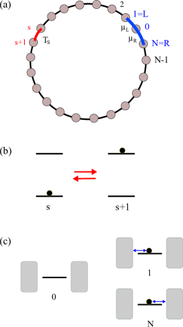
Figure 1: (color online). (a) A simple graph (model SC) representing an ideal (no non-radiative losses) photovoltaic cell. The system is driven away from equilibrium by the processes that take place at the red and blue segments. (b) Dynamics at the red segment: States $s$ and $s+1$ are ground and excited states of a dye molecule and transition between them is driven by the “sun temperature” $T_{S}$. (c) Dynamics at the blue segment. The transitions $0\rightleftharpoons 1$ and $0\rightleftharpoons N$ represent changes in the number of electrons on the molecule due to its coupling to the left and right electrodes, respectively. Non-equilibrium is imposed by the voltage difference $V$ between the two electrodes, $\mu_{R}-\mu_{L}=V$ (the electron charge $e$ is set to $1$ here and below).

An example is shown in Fig. 1 that depicts a single cycle model (henceforth referred to as model SC) for a photovoltaic cell comprising $N$ states that represent a charge carrier occupying different sites in the system and one state (denoted $0$) in which the charge carrier is absent. Transition rates between system states $j=0,1,\cdots,N,$ are determined by state energies $E_{j}$, the bias voltage $V$ and the local temperatures. The latter are taken equal to ambient temperature $T$ everywhere except at the $s\rightleftharpoons s+1$ transition that is driven by the sun temperature $T_{S}$. The different rates satisfy detailed balance conditions:

$$\frac{k_{j+1,j}}{k_{j,j+1}} =e^{-\beta\left(E_{j+1}-E_{j}\right)}$$ (1)

for all $j$, $j+1$ except

$$\frac{k_{s+1,s}}{k_{s,s+1}}=e^{-\beta_{S}\left(E_{s+1}-E_{s}\right)}\qquad\qquad\qquad\textrm{(red segment)}$$ (2)

$$\frac{k_{1,0}}{k_{0,1}}=e^{-\beta\left(E_{1}-\mu_{L}\right)};\,\frac{k_{N,0}}{k_{0,N}}=e^{-\beta\left(E_{N}-\mu_{R}\right)}\;\;\textrm{(blue segment)}$$ (3)

where $k_{i,j}$ is the rate coefficient for the $j\rightarrow i$ transition and $\beta=(k_{B}T)^{-1}$, $\beta_{\rm S}=(k_{B}T_{\rm S})^{-1}$. The cycle affinity $\mathcal{A}$ is defined by Schnakenberg (1976)

$$\mathcal{A} =-\ln\mathcal{K}$$ (4)

where $\mathcal{K}$ is the ratio between products of forward and backward rates

$$\mathcal{K} =\frac{k_{0,N}k_{N,N-1}\cdots k_{2,1}k_{1,0}}{k_{N,0}k_{N-1,N}\cdots k_{1,2}k_{0,1}}\,.$$ (5)

The open-circuit (OC) voltage is determined by the condition that the drivings associated with the voltage $V$ and with the difference between $T$ and $T_{\rm S}$ balance each other so that the steady state current through the system vanishes. In this case, the cycle affinity vanishes Einax and Nitzan (2014), namely $\mathcal{K}=1$. Denoting the corresponding voltage $\mu_{R}-\mu_{L}$ by $V_{\rm OC}$ and using Eqs. (1)-(3) this leads to

$$\frac{V_{\rm OC}}{\Delta E}=1-\frac{T}{T_{S}}\equiv\eta_{C}\,;\quad\Delta E=E_{s+1}-E_{s}\,.$$ (6)

The l.h.s is $\lim_{J\rightarrow 0}\eta(J)$ where $\eta(J)=V(J)/\Delta E$ is the thermodynamic (“internal”) efficiency of the device and $J$ is the steady state current (same through all links). Equation (6) thus yields the Carnot expression $\eta_{C}$ for the efficiency in the zero power limit. It also highlights the OC voltage as an important attribute in the quest to understand cell performance Vandewal et al. (2009); Kirchartz et al. (2009); Potscavage et al. (2009); Nayak et al. (2011). In Ref. Einax et al., 2011 we have derived two important generalizations of this result: First, if the transition $s\rightleftharpoons s+1$ results from the combinations of radiative and non-radiative processes whose forward/backward ratios are determined by temperatures $T_{\rm S}$ and $T$, respectively, Eq. (6) is replaced by a similar expression in which $T_{\rm S}$ is substituted by an effective temperaturenot (a)

$$T_{\rm eff} =T_{\rm S}\left(1+\frac{k_{\rm B}T}{\Delta E}\ln\left[\frac{1+\rho}{1+\rho\exp[-(\beta-\beta_{\rm S})\Delta E]}\right]\right)^{-1}$$

$$\simeq T_{\rm S}\left(1+\frac{k_{\rm B}T}{\Delta E}\ln[1+\rho]\right)^{-1}\,,$$

where $\rho=k_{s,s+1}^{\rm NR}/k_{s,s+1}^{\rm R}$ is the ratio between the non-radiative and radiative relaxation rates. Second, if one of the cycle processes involves charge separation that comes at an energy cost (exciton binding energy) $E_{B}$, Eq. (6) is replaced by Einax and Nitzan (2014)

$$\frac{V_{\rm OC}}{\Delta E} =\eta_{C}-\frac{E_{B}}{\Delta E}\,.$$ (7)

The later situation characterizes the operation of organic photovoltaic cells Giebink et al. (2011); Koster et al. (2012); Gruber et al. (2012).

Model SC and Eqs. (4)-(7) constitute a convenient framework for analyzing the OC voltage of photovoltaic cells, and, as shown in Ref. Einax and Nitzan, 2014, can be used as a starting point for studying optimal performance in finite power operations, provided that information on the system electronic structure and dynamics can be incorporated into such state-space model. However, this single cycle model is oversimplified; realistic state-space models contain intersecting pathways that makes the analysis that leads to Eqs. (4)-(6) more involved. Indeed, in state-space models of photovoltaic cells such intersecting pathways represent non-radiative losses, e.g., electron-hole recombination processes that are expected to reduce efficiency.

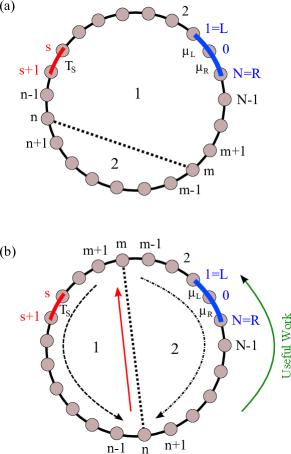
Figure 2: (color online). Models characterized by intersected graphs - an new pathway is added between sites $m$ and $n$. (a) The intersecting pathway does not separate the two driving (red and blue) segments. (b) The bond $n-m$ separates between the two driving segments which now sit on different subcycles.

As graphical structures, such intersecting pathways divide the cycle of model SC into separate cycles (see Fig. 2), making it possible to have steady states in which the current in the power-extracting segment vanishes while internal currents exist elsewhere in the system. While intuitively we expect lower efficiencies in such situations, no general proof for this is available.

In this Letter we consider two generalizations of model SC shown in Fig. 2. In one [Fig. 2(a)], an intersecting pathway divides the system cycle into two subcycles without separating between the two driving segments. In the second [Fig. 2(b)], the driving segments are positioned on different cycles. We show that (a) Intersecting pathways of the type shown in Fig. 2(a) do not affect the OC voltage, hence their zero power operation is characterized by the Carnot efficiency. (b) Intersecting pathways of the type shown in Fig. 2(b) lead to zero power efficiency smaller that the Carnot value, manifested for photovoltaic cells be a lower OC voltage.

We start with Model SC and take note of the two sites, $m$ and $n$, between which a new pathway will be enabled. The rate ratio, Eq. (5), can obviously be written as $\mathcal{K}=\bar{\mathcal{K}}_{1}\bar{\mathcal{K}}_{2}$ where $\bar{\mathcal{K}}_{1}=k_{n,n-1}\cdots k_{m+1,m}/k_{n-1,n}\cdots k_{m,m+1}$ and $\bar{\mathcal{K}}_{2}=k_{m,m-1}\cdots k_{n+1,n}/k_{m-1,m}\cdots k_{n,n+1}$ are ratios of rate products that correspond to the arcs $1$ and $2$ in Fig. 2. Now enable the pathway between sites $n$ and $m$, that is, make $k_{n,m}$ and $k_{m,n}$ different from zero. The graph is now divided into two subcycles, $1$ and $2$ in addition to the original cycle. The corresponding cycle rate-product ratios are

$$\mathcal{K}_{1} =\bar{\mathcal{K}}_{1}\frac{k_{m,n}}{k_{n,m}}\,;\quad\mathcal{K}_{2}=\bar{\mathcal{K}}_{2}\frac{k_{n,m}}{k_{m,n}}$$ (8)

so that $\mathcal{K}_{1}\mathcal{K}_{2}=\bar{\mathcal{K}}_{1}\bar{\mathcal{K}}_{2}$.

Consider next the situation shown in Fig. 2(a), where the two driving segments are on the same subcycle $1$. Starting from the model SC in the OC situation so that $\mathcal{K}=\mathcal{K}_{1}\mathcal{K}_{2}=1$, enabling the $n-m$ link does not lead to current on this bond. To show this note that since all rates on arc $2$ satisfy Eq. (1), we have $\bar{\mathcal{K}}_{2}=e^{-\beta(E_{m}-E_{n})}=k_{m,n}/k_{n,m}$. Equation (8) then yields $\mathcal{K}_{2}=1$ and therefore $\mathcal{K}_{1}=1$. Consequently, connecting the sites $n$ and $m$ will not create any extra current and subsequently does not affect the open-circuit voltage.

In the situation of Fig. 2(b), each of the subcycles created by enabling the $n-m$ pathway contains a non-equilibrium element: driving by the sun in subcycle $1$ and the driving by the voltage in subcycle $2$. Focusing on the latter and using Eqs. (1) and (3) yields

$$\bar{\mathcal{K}}_{2} =e^{-\beta(E_{m}-E_{n})}e^{-\beta\Delta\mu}=\frac{k_{m,n}}{k_{n,m}}e^{-\beta\Delta\mu}\,,$$ (9)

where $\Delta\mu=\mu_{R}-\mu_{L}$. Equation (8) then yields $\mathcal{K}_{2}=\exp[-\beta\Delta\mu]$. This indicates that with the $m-n$ link enabled the system cannot establish a state where currents through all links in subcycle $2$ vanish unless $\Delta\mu=0$.

To understand the consequence for the open-circuit voltage, let us set $k_{n,m}=\lambda\bar{k}_{n,m}$ and $k_{m,n}=\lambda\bar{k}_{m,n}$ and evaluate the derivative of the OC voltage, $V_{\rm OC}$, with respect to $\lambda$ at $\lambda=0$. $V_{\rm OC}$ is the value of $\Delta\mu=\mu_{R}-\mu_{L}$ for which the current between the electrodes, (the blue segment in Figs. 1 and 2), therefore across all links in arc $1$, vanishes; namely $k_{j,j+1}P_{j+1}=k_{j+1,j}P_{j}$ for all this links. From Eqs. (1) and (3) it follows that under OC conditions, the probabilities to find the system in states $n$ and $m$ are related to $V_{\rm OC}$ by

$$\frac{{P}_{m}}{{P}_{n}} =e^{-\beta(V_{\rm OC}+E_{m}-E_{n})}\,.$$ (10)

It follows that

$$\left(\frac{dV_{\rm OC}}{d\lambda}\right)_{\lambda=0}=-c\left(\frac{d}{d\lambda}\frac{\bar{P}_{m}}{\bar{P}_{n}}\right)_{\lambda=0}$$ (11)

where $c$ is a positive number and $P_{j}=\bar{P}_{j}e^{-\beta E_{j}}$. The derivative on the r.h.s is negative if ($\bar{P}_{m}>\bar{P}_{n})_{\lambda=0}$, i.e. $V_{\rm OC}<0$, and negative in the opposite case, ($\bar{P}_{m}<\bar{P}_{n})_{\lambda=0}$; $V_{\rm OC}>0$ (this can be inferred from the current expression, $J_{n\leftarrow m}=\lambda\left(\bar{k}_{n,m}P_{m}-\bar{k}_{m,n}P_{n}\right)=\lambda\bar{k}_{n,m}e^{-\beta E_{m}}\left(\bar{P}_{m}-\bar{P}_{n}\right)$. Hence

$$\left(\frac{d|V_{\rm OC}|}{d\lambda}\right)_{\lambda=0}<0\,.$$ (12)

Enabling the $m-n$ link in the scheme of Fig. 2(b) thus results in reduction of the OC voltage, namelt of the maximum thermodynamic efficiency.

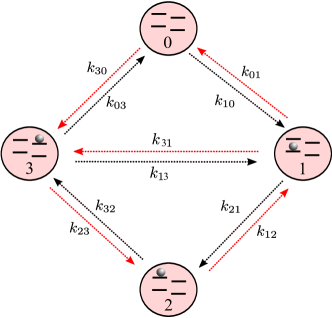
Figure 3: (color online). A $4$-level spinless model of an organic photovoltaic cellEinax et al. (2011, 2013). The states are: $0$ - no excess electron, $1$ - excess electron in the higher occupied molecular orbital (HOMO) of the donor, $2$ - Following an optical transition, electron is on the otherwise lower unoccupied molecular orbital (LUMO) of the donor (an exciton state). $3$: Following charge separation, the electron has moved to the acceptor LUMO. The transitions $3\rightleftharpoons 0$ and $0\rightleftharpoons 1$ include electron transfer to the right and left electrode, respectively, $1\rightleftharpoons 2$ is the optical excitation process and $2\rightleftharpoons 3$ is the exciton dissociation process (see Ref. Einax et al., 2011 for further details). The process $3\rightleftharpoons 1$ that divides the cycle to two subcycles represents radiationless recombination.

To illustrate this general observation for a particular system, we consider a simple $4$-level model for an organic photovoltaic cell comprising a donor acceptor (D-A) complex placed between two electrodes (see Fig. 3 and Supplementary Material not, b). The $D$ and $A$ species are characterized by their HOMO levels, $\varepsilon_{\rm D_{H}}$, $\varepsilon_{\rm A_{H}}$, and LUMO levels, $\varepsilon_{\rm D_{L}}$, $\varepsilon_{\rm A_{L}}$ that translate into three relevant energy differences $\Delta E=\varepsilon_{\rm D_{L}}-\varepsilon_{\rm D_{H}}$ (the optical gap), $\Delta\epsilon=\varepsilon_{\rm D_{L}}-\varepsilon_{\rm A_{L}}$ (interfacial LUMO-LUMO gap), and $E_{DA,g}=\varepsilon_{\rm A_{L}}-\varepsilon_{\rm D_{H}}$ (effective band gap). Charge carriers can enter and leave the system only by transitions between the donor HOMO level and the electrode $L$, and between the acceptor LUMO level and the electrode $R$. These electrodes are represented by free-electron reservoirs at chemical potentials $\mu_{K}$ ($K=L;R$). An important feature of this model is that a thermal fluctuation is needed to overcome the exciton binding energy $E_{B}$ of an interfacial charge transfer exciton to generate a free charge carrier. With some simplifying assumptions, the system can be described by a kinetic scheme involving four states. A detailed description of this model and the underlying kinetic scheme was given in Ref. Einax et al., 2011.

An additional link between states $1$ and $3$ correspond to non-radiative recombination that returns a free electron on the acceptor back to the donor ground state. In the absence of this process, the open-circuit voltage $V_{\rm OC}(\lambda=0)$ is found to be given by Eq. (7). The maximum thermodynamic efficiency is correspondingly $\eta_{C}-E_{B}/\Delta E$, highlighting the loss associated with the exciton binding energy.

Repeating the cycle analysis when the rates $k_{13}$, $k_{31}$ are finite not (b) yields the following expression for the open-circuit voltage

$$V_{\rm OC}(\lambda) =\Delta E\eta_{C}-E_{B}-k_{B}T\ln\frac{\displaystyle 1+k_{13}\frac{k_{12}+k_{32}}{k_{12}k_{23}}}{\displaystyle 1+k_{31}\frac{k_{12}+k_{32}}{k_{21}k_{32}}}\,,$$ (13)

setting $k_{13}=\lambda\overline{k}_{13}$ and $k_{31}=\lambda\overline{k}_{31}$. and taking the derivative with respect to $\lambda$ we find, using also Eqs.(S5-S8)

$$\left(\frac{dV_{\rm OC}}{d\lambda}\right)_{\lambda=0} =-k_{B}T\frac{\overline{k}_{13}(k_{32}+k_{12})}{k_{12}k_{23}}\left(1-e^{-\beta(V_{\rm OC})_{\lambda=0}}\right)\,.$$ (14)

where $(V_{\rm OC})_{\lambda=0}$ is given by (7). This is an explicit statement of the inequality (12).

In conclusion, we have presented a state-space network representation scheme of molecular scale engines and applied it to models of photovoltaic cells. A general argument based on cycle analysis yields conditions under which the opening of intersecting pathways in an otherwise cyclical graph leads to a decrease in the maximum efficiency. In the application to the operation of a photovoltaic cell such intersecting link often corresponds to a carrier recombination process, and its consequence is manifested in a reduced open-circuit voltage. It should be emphasized that similar analysis can be carried out for more complex models that include, for example, polaron formation and hot exciton dissociation, as well as for other types of nano-scale engines, provided that they can be modeled by kinetic transitions in the system state-space. As described elsewhere Einax and Nitzan (2014), such an approach can be used for analysis of optimal performance under finite power operation, although with the unavoidable loss of the generality associated with a thermodynamic description.

References

- Seifert (2012) U. Seifert, Rep. Prog. Phys. 75, 126001 (2012).
- Hill (1966) T. L. Hill, Journal of Theoretical Biology 10, 442 (1966).
- Hill (2009) T. L. Hill, Free Energy Transduction and Biochemical Cycle Kinetics, 2nd ed. (Dover, New York, 2009).
- Gerritsma and Gaspard (2010) E. Gerritsma and P. Gaspard, Biophysical Reviews and Letters 05, 163 (2010).
- Schnakenberg (1976) J. Schnakenberg, Rev. Mod. Phys. 48, 571 (1976).
- Einax and Nitzan (2014) M. Einax and A. Nitzan, J. Phys. Chem. C 118, 27226 (2014).
- Vandewal et al. (2009) K. Vandewal, K. Tvingstedt, A. Gadisa, O. Inganas, and J. V. Manca, Nat. Mater. 8, 904 (2009).
- Kirchartz et al. (2009) T. Kirchartz, K. Taretto, and U. Rau, J. Phys. Chem. C 113, 17958 (2009).
- Potscavage et al. (2009) W. J. Potscavage, A. Sharma, and B. Kippelen, Acc. Chem. Res. 42, 1758 (2009).
- Nayak et al. (2011) P. K. Nayak, J. Bisquert, and D. Cahen, Adv. Mater. 23, 2870 (2011).
- Einax et al. (2011) M. Einax, M. Dierl, and A. Nitzan, J. Phys. Chem. C 115, 21396 (2011).
- not (a) This result is obtained from Eq. (26) of Ref.Einax and Nitzan, 2014 by using the detailed balance relationships between the different rates.
- Giebink et al. (2011) N. C. Giebink, G. P. Wiederrecht, M. R. Wasielewski, and S. R. Forrest, Phys. Rev. B 83, 195326 (2011).
- Koster et al. (2012) L. J. A. Koster, S. E. Shaheen, and J. C. Hummelen, Adv. Energy Mater. 2, 1246 (2012).
- Gruber et al. (2012) M. Gruber, J. Wagner, K. Klein, U. Hörmann, A. Opitz, M. Stutzmann, and W. Brütting, Adv. Energy Mater. 2, 1100 (2012).
- Einax et al. (2013) M. Einax, M. Dierl, P. R. Schiff, and A. Nitzan, Europhys. Lett. 104, 40002 (2013).
- not (b) See Supplemental Material at http://[.].