Chimera-Like Coexistence of Synchronized Oscillation and Death in an Ecological Network

Abstract

We report a novel spatiotemporal state, namely the chimera-like incongruous coexistence of synchronized oscillation and stable steady state (CSOD) in a realistic ecological network of nonlocally coupled oscillators. Unlike the chimera and chimera death state, in the CSOD state identical oscillators are self-organized into two coexisting spatially separated domains: In one domain neighboring oscillators show synchronized oscillation and in another domain the neighboring oscillators randomly populate either a synchronized oscillating state or a stable steady state (we call it a death state). We show that the interplay of nonlocality and coupling strength results in two routes to the CSOD state: One is from a coexisting mixed state of amplitude chimera and death, and another one is from a globally synchronized state. We further explore the importance of this study in ecology that gives a new insight into the relationship between spatial synchrony and global extinction of species.

Understanding of collective dynamical behaviors in networks of coupled oscillators has been an active area of extensive research in the field of physics, chemistry, biology, engineering and social sciences. Coupled oscillators show a plethora of cooperative phenomena, such as synchronization Strogatz (2012), amplitude death Saxena et al. (2012), oscillation death Koseska et al. (2013a), chimera Panaggio and Abrams (2015), chimera death Zakharova et al. (2014), etc. Two intriguing spatiotemporal dynamical states, namely the chimera and the recently observed chimera death have been in the center of recent research on coupled oscillators for their rich complex behaviors.

The chimera state is a fascinating spatiotemporal state where synchronous and asynchronous oscillations coexist in a network of coupled identical oscillators. After its discovery by Kuramoto and Battogtokh (2002) and mathematical proof in Ref. Abrams and Strogatz (2004); *st2, the chimera state attracts immediate attention due to its possible connection with unihemispheric sleep in certain species Panaggio and Abrams (2015), the multiple time-scales of sleep dynamics Olbrich et al. (2011), etc. Unlike phase chimera, where chimera occurs in the phase part, recently it is found that in the strong coupling limit amplitude effects come into play that results in amplitude mediated chimera Sethia and Sen (2014); *sethia2 and amplitude chimera Zakharova et al. (2014), Omelchenko et al. (2011); *scholl3. The existence of chimera has also been established in many experiments, e.g., in optical system Hagerstrom et al. (2012), chemical oscillators Tinsley et al. (2012), mechanical system Martens et al. (2013), and electronic system Gambuzza et al. (2014). Further, chimera state has been observed in various fields; examples include Omelchenko et al. (2013); *chiex2; *chiex3: FitzHugh-Nagumo oscillator, the SNIPER model of excitability of type-I, autonomous Boolean networks, etc (for an elaborate review please see Panaggio and Abrams (2015)). Recently, chimera state in population dynamics is observed using Lattice Limit Cycle (LLC) model Hizanidis et al. (2015).

On the other hand, the chimera death (CD) state is discovered very recently by Zakharova et al. (2014) in a network of Stuart-Landau oscillators under nonlocal coupling. The CD state connects the chimera state to the oscillation death (OD) state Koseska et al. (2013b). In the OD state oscillators populate different branches of a stable inhomogeneous steady state (IHSS) Koseska et al. (2013a); *tanpre1; *tanpre2; *tanpre3. According to Ref.Zakharova et al. (2014), in the chimera death state the population of oscillators in a network splits into coexisting domains of spatially coherent OD (where neighboring nodes attain essentially the same branch of the IHSS) and spatially incoherent OD (where the neighboring nodes jump among the different branches of IHSS in a completely random manner). Later, CD is also found in a network of mean-field diffusively coupled oscillators Banerjee .

In summary, the chimera state is a spatial coexistence of coherent and incoherent oscillations, and the chimera death state is a spatial coexistence of coherent and incoherent branches of oscillation death state. Thus, the next natural question arises: Is it possible to have an emergent state in a network of oscillators that shows a chimera-like coexistence of coherent oscillation and stable steady state?

In this Letter, for the first time, we indeed find the answer in affirmative. Here, we address this open question and show that in a realistic ecological network consists of Rosenzweig–MacArthur oscillators Rosenzweig and MacArthur (1963) under nonlocal coupling topology, the interplay of non locality and coupling strength gives rise to a novel spatiotemporal state. In this state, the population of oscillators split into two coexisting distinct spatially separated domains: In one domain oscillators are oscillating in synchrony (i.e., coherently), and in another domain neighboring oscillators depict spatially synchronized oscillation and stable steady state in a random manner (i.e., incoherently). Hereafter, we call this hitherto unobserved state a chimera-like synchronized oscillation and death (CSOD) state (the stable steady state is denoted as a death state). Depending upon the coupling range and coupling strength, we identify two types of transitions to the CSOD state: With increasing coupling range (for a moderate coupling strength) the CSOD state arises from a coexisting mixed state of amplitude chimera and death state; on the other hand, for an increasing coupling strength (with a moderate coupling range) the CSOD state comes from a globally synchronized oscillation state. However, in both the cases, under large coupling range and strength, the CSOD state is transformed into a chimera death state. Thus, the CSOD state bridges the gap between the amplitude chimera and the chimera death state. We further discuss the ecological importance of this emergent behavior that gives us a new insight into the relationship between spatial synchrony and global extinction of species, which are thought of as closely connected phenomena in ecology Heino et al. (1997); *EaRoGr98; *EaLeRo00; *LiKoBj04; *gr: Spatial synchrony may lead to global extinction of species. Here we show that our results differ from this general consensus, and local extinction of a species does not necessarily lead to a global extinction of that species.

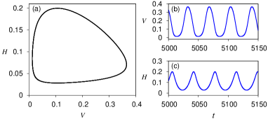
Figure 1: (Color online) (a) Limit cycle attractor, and (b), (c) time-series of the uncoupled Rosenzweig–MacArthur model given by Eqs. (1) for $r=0.5$, $K=0.5$, $\alpha=1$, $B=0.16$, $\beta=0.5$ and $m=0.2$.

Here we consider the following network of $N$ identical nonlocally coupled Rosenzweig–MacArthur (RM) oscillators:

$$\frac{dV_{i}}{dt} =rV_{i}\left(1-\frac{V_{i}}{K}\right)-\frac{\alpha V_{i}}{V_{i}+B}H_{i},$$ (1a)

$$\frac{dH_{i}}{dt} =H_{i}\left(\frac{\alpha\beta V_{i}}{V_{i}+B}-m\right)+\frac{\sigma}{2P}\sum_{k=i-P}^{i+P}\left(H_{k}-H_{i}\right),$$ (1b)

with $V$ and $H$, respectively, representing vegetation and herbivore density, interacting in $i~{}(=1,2,\cdots,N)$ discrete patches (or nodes) (“$i$” is taken as modulo $N$). The local dynamics in each node are governed by the following system parameters: $r$ is the intrinsic growth rate, $K$ is the carrying capacity, $\alpha$ is the maximum predation rate of the herbivore, $B$ is the half saturation constant, $\beta$ represents the herbivore efficiency and $m$ is the mortality rate of the herbivore. Interaction between nodes is governed by two coupling parameters: $\sigma$ is the coupling strength and $P$ controls the coupling range, where $1\leq P\leq\frac{N}{2}$. Two limiting values of $P$, i.e., $P=1$ and $P=N/2$ represent local and global coupling, respectively. This nonlocal coupling topology has been used in Ref. Zakharova et al. (2014) and Ref. Omelchenko et al. (2011); *scholl3 to observe chimera states in periodic and chaotic oscillators. The Rosenzweig–MacArthur model perhaps is the simplest model that can actually be applied in real ecosystems. As a result, this model becomes a standard spatially structured prey–predator model in theoretical ecology Holland and Hastings (2008); *GoHa09; *GoHa11; Banerjee et al. (2015).

An individual RM oscillator [see Eqs. (1) for $\sigma=0$ and a fixed $i$] has the following steady states: (i) $(V^{*},H^{*})=(0,0)$, the eigenvalues are $\lambda=r$, $-m$ and the equilibrium point is a saddle point, (ii) $(V^{*},H^{*})=(K,0)$, the eigenvalues are $\lambda=-r$, $-m+\alpha\beta\frac{K}{K+B}$ and the equilibrium point is either a stable node or a saddle node, depending upon the values of the parameters, and finally (iii) $(V^{*},H^{*})=(\frac{mB}{\alpha\beta-m},\frac{r}{\alpha}(1-\frac{mB}{K(\alpha\beta-m)})(\frac{B\alpha\beta}{\alpha\beta-m}))$; this nontrivial equilibrium point is stable for parameter values satisfying the inequality $\frac{B}{K}<\frac{(\alpha\beta-m)}{(\alpha\beta+m)}$. Beyond a certain $K$, this equilibrium point becomes unstable and gives rise to a stable limit cycle through Hopf bifurcation. In general, further increase in $K$ gradually increases amplitude of the limit cycle, thus bringing the density of either the prey or the predator or both the populations closer to zero, eventually leading to the extinction of the ecosystem; this is known as “the paradox of enrichment” Rosenzweig (1971) proposed by M. L. Rosenzweig in 1971. A subsequent realistic range Murdoch et al. (1998) of $K$ is $0.15$ to $3$ and range of $m$ is $0.03$ to $0.41$. In Fig. 1, a stable limit cycle is shown for the following parameter values: $r=0.5$, $K=0.5$, $\alpha=1$, $B=0.16$, $\beta=0.5$ and $m=0.2$.

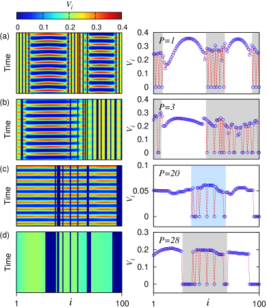
Figure 2: (Color online) Left panel: Spatiotemporal color map and right panel: $V_{i}$ with oscillator index “$i$” [red (dotted) line is for visual guidance]. Coupling strength $\sigma=1.7$, $N=100$. (a) $P=1$ ($\gamma=0.01$) and (b) $P=3$ ($\gamma=0.03$) show the mixed state of amplitude chimera and stable zero steady state (gray shade in right panels are for visual guidance). (c) $P=20$ ($\gamma=0.2$): Chimera-like synchronized oscillation and death (CSOD) state. Cyan (gray) shaded region in the right panel shows the random sequential occurrence of the synchronized oscillation and zero steady state of the neighboring nodes. (d) $P=28$ ($\gamma=0.28$): The chimera death state. Initial time $t=5000$ is discarded before presenting the figures. Other parameters are same as used in Fig.1.

To explore various spatiotemporal patterns in the network, we take $N=100$ and integrate Eqs. (1) numerically . While presenting the simulation results, a large number of initial integration time ($t=5000$) is discarded in order to ensure the steady state behavior. At first, we consider a moderate coupling strength, $\sigma=1.7$, and increase the coupling range, $\gamma=P/N$, from a lower value. For lower coupling range ($\gamma\leq 0.05$) we observe a mixed state comprises of amplitude chimera and stable zero steady state (i.e., death state). This is shown in Figs. 2(a) and 2(b) for $\gamma=0.01$ and $\gamma=0.03$, respectively. The left panel in Fig. 2 shows the space-time color map of $V_{i}$ and the right panel shows $V_{i}$ in the steady state with oscillator index (“$i$”). The gray shaded regions in Figs. 2(a) and 2(b) (right panel) show this mixed state of amplitude chimera and death: the amplitude chimera interrupted by death state is a new observation in the context of coupled oscillators. Further increase in coupling range $\gamma$ results in the CSOD state where the population of oscillators splits into two distinct coexisting domains: In one domain the neighboring nodes oscillate in synchrony while in another domain the neighboring nodes randomly populate either the synchronized oscillating state or the stable steady (death) state. This new spatiotemporal state is shown in Fig. 2(c) for $\gamma=0.2$ (i.e., $P=20$). Here we see that in the shaded region [right panel of Fig. 2(c)] the neighboring oscillators populate either synchronized oscillation state or stable zero steady state in a random sequence. However, in the non shaded region only synchronized oscillation exists except in the rightmost nodes where few oscillators attain the death state. To the best of our knowledge, this chimera-like spatiotemporal state is new in literature because here stable steady state coexists with synchronized oscillations, which is unlike the chimera state or chimera death state. We also verify that this CSOD state is preserved for a larger number of nodes, $N$ . If we further increase the coupling range, we find the chimera death state [Fig. 2(d) for $\gamma=0.28$]. We notice that instead of populating two branches of OD Zakharova et al. (2014), Banerjee , denoted as lower and upper branch, here in the CD state, the OD state has more than two branches [later it is clearly shown in Fig. 5(b)]. The multiple-branches (more than two) of OD was reported earlier in Koseska and Kurths (2010) for sixteen locally coupled genetic relaxation oscillators, but in a network of large number of oscillators with nonlocal coupling it is an important observation (to be discussed later on).

We also identify one more significant route to the CSOD state with increasing coupling strength ($\sigma$) and a fixed $\gamma$, namely the transition from a global in-phase synchronized oscillating state to the CSOD state. This transition is shown in Figs. 3(a) and 3(b) for $\sigma=0.5$ and $\sigma=2.4$, respectively (for $\gamma=0.1$, i.e., $P=10$). Here also, the CSOD state is transformed into a multi-branch chimera death state for higher coupling strength (not shown).

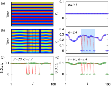
Figure 3: (Color online) Left panel: Spatiotemporal color map (color bar same as Fig. 2), and right panel: $V_{i}$ with oscillator index “$i$”. Coupling range $\gamma=0.1$ (i.e., $P=10$), $N=100$. (a) $\sigma=0.5$: Global in-phase synchronized oscillation. (b) $\sigma=2.4$ : The CSOD state. Cyan (gray) shaded region is for visual guidance of the incoherent region. (c) Standard deviation (S.D.) ($\Delta_{i}$) with index “$i$” for the CSOD state of Fig. 2(c). (d) $\Delta_{i}$ with index “$i$” for the CSOD state of Fig. 3(b). Other parameters are same as used in Fig.1.

Next, we quantify the spatiotemporal behavior where synchronized oscillation and stable zero steady (death) state coexist. In order to distinguish between the oscillation and death, we compute the standard deviation (S.D.) of each node given by:

$$\Delta_{i}=\sqrt{\left(<V_{i}^{2}>-<V_{i}>^{2}\right)}.$$ (2)

The “$<\;>$” sign denotes the time average, which is carried out over a long time period ($t=3000$ in the steady state). For a stable steady state (i.e., a death state) S.D. ($\Delta_{i}$) must be zero and in the oscillatory condition it will show a finite non-zero value. Figures 3(c) and 3(d) show $\Delta_{i}$ values of the CSOD states shown in Fig. 2(c) and Fig. 3(b), respectively. For the CSOD state, in the incoherent region, we see that the $\Delta_{i}$ changes from a finite non-zero value to zero in a random manner; in the populations where nodes are oscillating in synchrony its value is non-zero and shows a continuous spatial variation.

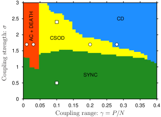
Figure 4: (Color online) Phase diagram in the $\gamma-\sigma$ space. CSOD: chimera-like synchronized oscillation and stable zero steady state (death); SYNC: Global in-phase synchronized oscillation; CD: Chimera death; AC+Death: Coexistence of amplitude chimera and stable zero steady state. The symbols $\circ$ indicate the coupling parameter values used for generating Figs. 2 (a)-2(d). $\Box$ represents the same for generating Figs. 3(a) and 3(b). Other parameters are same as used in Fig.1.

In order to reveal the complete spatiotemporal scenario of the considered network, we rigorously compute the phase diagram in the $\gamma-\sigma$ space (the unsynchronized zone with very small $\sigma$ value is not shown). From the phase diagram [Fig. 4] it is clear that the region of occurrence of the CSOD state is broad enough. It is seen that beyond $\gamma\approx 0.37$ (i.e., $P\approx 37$) no CSOD occurs; here an increase in $\sigma$ transforms the synchronized oscillation state (SYNC) directly to the chimera death. The symbols $\circ$ in the phase diagram indicate the coupling parameter values used for generating Figs. 2(a)-2(d), whereas $\Box$ represents the same for generating Figs. 3(a) and 3(b). In this context, it should be noted that in the phase diagram the boundaries among different phases are not very sharp, they tend to change with initial conditions. However, we observe that the overall qualitative structure of the phase diagram is preserved for all the initial conditions or number of nodes.

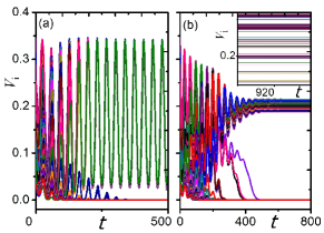
Figure 5: (Color online) Time series of $V_{i}$’s for (a) $\gamma=0.2$ and $\sigma=1.7$: Synchronized limit-cycle oscillation (upper branch) and stable zero steady state (i.e., $V=0$) coexists. (b) $\gamma=0.28$ and $\sigma=1.7$: Temporally stable multi-branch OD; Inset shows the multiple branches around $V_{i}=0.2$. Other parameters are same as used in Fig.1.

Next, we provide a qualitative explanation of the genesis of the CSOD state. We find that it has a strong connection with the inhomogeneous limit-cycle (IHLC) state in a network Tyson and Kauffman (1975); *kosihlc1, Ullner et al. (2007); IHLC is defined as a state where some nodes are in a stable steady state (or quasisteady state with a negligible amplitude, as in Ullner et al. (2007)), while the rest undergo oscillations. To visualize the scenario, we plot the time series of all the $V_{i}$’s [Fig. 5(a)] for an exemplary value of $\gamma=0.2$ and $\sigma=1.7$. From Fig. 5(a) one observes that a population of oscillators occupy the trivial zero steady state (i.e., $V=0$ state), while the rest of the oscillators are in the in-phase synchronized oscillating state. Thus, depending upon judiciously chosen spatial initial conditions, individual nodes may populate either the upper oscillating branch or the lower steady state (i.e., $V=0$) branch in a random sequence, which results in the CSOD state [as shown in Fig. 2(c)]. For higher coupling range and strength, e.g., $\gamma=0.28$ and $\sigma=1.7$, oscillators populate the multi-branch OD state [Fig. 5(b), see also the inset]; here a set of proper spatial initial conditions should result in chimera death in the network [as shown in Fig. 2(d)]. Thus, we may conjecture that, the CSOD state may occur in systems where this type of [Fig. 5(a)] IHLC state exists.

Finally, we discuss the importance of the results in ecology. In spatial ecology nonlocal coupling arises under the assumption that all spatially separated patches (or nodes) are connected only to certain number of neighboring nodes in a fragmented landscape, which is a more natural coupling scheme than the global coupling. In ecology, it is generally believed that spatial synchrony and global extinction are two strongly correlated phenomena (see for example, Refs.Heino et al. (1997); *EaRoGr98; *EaLeRo00; *LiKoBj04; *gr). In contrast to this general belief, in the present study we show that, in nonlocal dispersive coupling, although spatial synchronization gives rise to local extinction of a species in one or more patches (or nodes) [i.e., the death state] but it defies the global extinction of the species (i.e., not all the oscillators go to the death state). Moreover, a general consensus in ecology is that, spatial synchrony and dispersal induced stability (or temporal stability) are two conflicting outcomes of dispersion among the population of patches. In the existing studies it is shown that dispersion among identical patches results in spatial synchrony; on the other hand, the combination of spatial heterogeneity and dispersion is necessary for dispersal-induced stability (Briggs and Hoopes, 2004; *Ab11). Here our results show that depending on coupling range and strength, spatial synchronization among identical patches (or nodes) leads to temporally stable multi-branch (more than two) IHSS and a cluster of them has non-zero steady states. Thus, to achieve temporal stability the patches need not to be heterogeneous but nonlocal coupling is sufficient. Further, the occurrence of the amplitude chimera interrupted by death is a new finding and its proper interpretation in ecology deserves further attention.

In conclusion, in this Letter we have reported a novel spatiotemporal state, the CSOD state, in a realistic ecological network with nonlocal coupling topology. In this state a subset of oscillators populate spatially synchronized oscillation and stable steady state in a random manner, and the rest of the oscillators oscillate in synchrony. This spatiotemporal state is unlike the chimera state (where coherent and incoherent oscillations coexist) and the chimera death state (where neighboring oscillators populate two branches of OD in coherent and incoherent manner). We have shown two coupling dependent transition routes to this CSOD state. We further qualitatively established the connection of this emergent state with the inhomogeneous limit-cycle state present in the network. We have discussed the ecological importance of the results, which reveals that spatial synchrony does not necessarily lead to global extinction of a species, which is in contrast to the general consensus. Apart from ecology, we believe that, the present study will improve our understanding of other physical networks, e.g., power grid and communication networks, where it is desirable that a failure of certain nodes does not lead to a complete blackout or a global system failure Motter et al. (2013); *grid2.

T.B. acknowledges financial support from SERB, Department of Science and Technology (DST), India (Grant No. SB/FTP/PS-005/2013).

References

- Strogatz (2012) S. H. Strogatz, Sync: How Order Emerges from Chaos In the Universe, Nature, and Daily Life (Hyperion, New York, 2012).
- Saxena et al. (2012) G. Saxena, A. Prasad, and R. Ramaswamy, Phys. Rep. 521, 205 (2012).
- Koseska et al. (2013a) A. Koseska, E. Volkov, and J. Kurths, Phys. Rep. 531, 173 (2013a).
- Panaggio and Abrams (2015) M. J. Panaggio and D. M. Abrams, Nonlinearity 28, R67 (2015).
- Zakharova et al. (2014) A. Zakharova, M. Kapeller, and E. Schöll, Phys. Rev. Lett. 112, 154101 (2014).
- Kuramoto and Battogtokh (2002) Y. Kuramoto and D. Battogtokh, Nonlinear Phenom. Complex Syst. 4, 380 (2002).
- Abrams and Strogatz (2004) D. M. Abrams and S. H. Strogatz, Phys. Rev. Lett. 93, 174102 (2004).
- Abrams et al. (2008) D. M. Abrams, R. Mirollo, S. H. Strogatz, and D. A. Wiley, Phys. Rev. Lett. 101, 084103 (2008).
- Olbrich et al. (2011) E. Olbrich, J. C. Claussen, and P. Achermann, Phil. Trans. R. Soc. A 369, 3884 (2011).
- Sethia and Sen (2014) G. C. Sethia and A. Sen, Phys. Rev. Lett. 112, 144101 (2014).
- Sethia et al. (2013) G. C. Sethia, A. Sen, and G. L. Johnston, Phys. Rev. E 88, 042917 (2013).
- Omelchenko et al. (2011) I. Omelchenko, Y. Maistrenko, P. Hövel, and E. Schöll, Phys. Rev. Lett. 106, 234102 (2011).
- Omelchenko et al. (2012) I. Omelchenko, B. Riemenschneider, P. Hövel, Y. Maistrenko, and E. Schöll, Phys. Rev. E 85, 026212 (2012).
- Hagerstrom et al. (2012) A. M. Hagerstrom, T. E. Murphy, R. Roy, P. Hövel, I. Omelchenko, and E. Schöll, Nat. Phys. 8, 658 (2012).
- Tinsley et al. (2012) M. R. Tinsley, S. Nkomo, and K. Showalter, Nat. Phys. 8, 662 (2012).
- Martens et al. (2013) E. A. Martens, S. Thutupalli, A. Fourrière, and O. Hallatschek, Proc. Natl. Acad. Sci. U.S.A. 110, 10563 (2013).
- Gambuzza et al. (2014) L. V. Gambuzza, A. Buscarino, S. Chessari, L. Fortuna, R. Meucci, and M. Frasca, Phys. Rev. E 90, 032905 (2014).
- Omelchenko et al. (2013) I. Omelchenko, O. Omelćhenko, P. Hövel, and E. Schöll, Phys. Rev. Lett. 110, 224101 (2013).
- Vüllings et al. (2014) A. Vüllings, J. Hizanidis, I. Omelchenko, and P. Hövel, New J. Phys. 16, 123039 (2014).
- Rosin et al. (2014) D. P. Rosin, D. Rontani, N. D. Haynes, E. Schöll, and D. J. Gauthier, Phys. Rev. E 90, 030902(R) (2014).
- Hizanidis et al. (2015) J. Hizanidis, E. Panagakou, I. Omelchenko, E. Schöll, P. Hövel, and A. Provata, arXiv 1504.08125 [nlin.CD] (2015).
- Koseska et al. (2013b) A. Koseska, E. Volkov, and J. Kurths, Phys. Rev. Lett. 111, 024103 (2013b).
- Banerjee and Ghosh (2014a) T. Banerjee and D. Ghosh, Phys. Rev. E 89, 052912 (2014a).
- Banerjee and Ghosh (2014b) T. Banerjee and D. Ghosh, Phys. Rev. E 89, 062902 (2014b).
- Ghosh and Banerjee (2014) D. Ghosh and T. Banerjee, Phys. Rev. E 90, 062908 (2014).
- (26) T. Banerjee, arXiv 1409.7895v1[nlin.CD].
- Rosenzweig and MacArthur (1963) M. L. Rosenzweig and R. H. MacArthur, Am. Nat. 97, 209 (1963).
- Heino et al. (1997) M. Heino, V. Kaitala, E. Ranta, and J. Lindström, Proc. R. Soc. B: Biol. Sci. 264, 481 (1997).
- Earn et al. (1998) D. J. D. Earn, P. Rohani, and B. T. Grenfell, Proc. R. Soc. B: Biol. Sci. 265, 7 (1998).
- Earn et al. (2000) D. J. D. Earn, S. A. Levin, and P. Rohani, Science 290, 1360 (2000).
- Liebhold et al. (2004) A. Liebhold, W. D. Koenig, and O. N. Bjornstad, Annu. Rev. Ecol. Evol. Syst. 35, 467 (2004).
- Amritkar and Rangarajan (2006) R. E. Amritkar and G. Rangarajan, Phys. Rev. Lett. 96, 258102 (2006).
- Holland and Hastings (2008) M. D. Holland and A. Hastings, Nature 456, 792 (2008).
- Goldwyn and Hastings (2009) E. E. Goldwyn and A. Hastings, Bull. Math. Biol. 71, 130 (2009).
- Goldwyn and Hastings (2011) E. E. Goldwyn and A. Hastings, J. of Theor. Biol. 289, 237 (2011).
- Banerjee et al. (2015) T. Banerjee, P. S. Dutta, and A. Gupta, Phys. Rev. E 91, 052919 (2015).
- Rosenzweig (1971) M. L. Rosenzweig, Science 171, 385 (1971).
- Murdoch et al. (1998) W. W. Murdoch, R. M. Nisbet, E. McCauley, A. M. deRoos, and W. S. C. Gurney, Ecology 79, 1339 (1998).
- Note (1) We use the fourth-order Runge-Kutta algorithm with step size .
- Note (2) See Supplemental Material at [URL will be inserted by publisher] for the CSOD state for .
- Koseska and Kurths (2010) A. Koseska and J. Kurths, Chaos 24, 045111 (2010).
- Tyson and Kauffman (1975) J. Tyson and S. Kauffman, J. Math. Biol. 1, 289 (1975).
- Ullner et al. (2010) E. Ullner, E. Ullner, E. I. Volkov, J. Kurths, and J. García-Ojalvo, J. Theor. Biol 263, 189 (2010).
- Ullner et al. (2007) E. Ullner, A. Zaikin, E. I. Volkov, and J. García-Ojalvo, Phys. Rev. Lett. 99, 148103 (2007).
- Briggs and Hoopes (2004) C. J. Briggs and M. F. Hoopes, Theor. Popul. Biol. 65, 299 (2004).
- Abbott (2011) K. C. Abbott, Ecol. Lett. 14, 1158 (2011).
- Motter et al. (2013) A. E. Motter, S. A. Myers, M. Anghel, and T. Nishikawa, Nature Physics 9, 191 (2013).
- Menck et al. (2014) P. J. Menck, J. Heitzig, J. Kurths, and H. J. Schellnhuber, Nature Comm. 5, 3969 (2014).