Compressed self-avoiding walks, bridges and polygons

Nicholas R Beaton Department of Mathematics and Statistics, University of Saskatchewan, Saskatoon, Canada Anthony J Guttmann School of Mathematics and Statistics, University of Melbourne, Victoria 3010, Australia Iwan Jensen School of Mathematics and Statistics, University of Melbourne, Victoria 3010, Australia Gregory F Lawler Department of Mathematics, University of Chicago, Chicago, Illinois, USA
Abstract

We study various self-avoiding walks (SAWs) which are constrained to lie in the upper half-plane and are subjected to a compressive force. This force is applied to the vertex or vertices of the walk located at the maximum distance above the boundary of the half-space. In the case of bridges, this is the unique end-point. In the case of SAWs or self-avoiding polygons, this corresponds to all vertices of maximal height. We first use the conjectured relation with the Schramm-Loewner evolution to predict the form of the partition function including the values of the exponents, and then we use series analysis to test these predictions.00footnotetext: Email: n.beaton@usask.ca, guttmann@unimelb.edu.au, i.jensen@ms.unimelb.edu.au, lawler@math.uchicago.edu

Dedicated to R.J. Baxter, for his 75th birthday.

Keywords: self-avoiding walk; Schramm-Loewner evolution; bridges; compressive force

1 Introduction

Self-avoiding walks (SAWs) were initially introduced [9, 28] as a model of long linear polymer chains. Since that time they have been explored both as a polymer model in statistical mechanics and as an independent problem of interest to combinatorialists and theoretical computer scientists.

In the simplest case, one considers walks on the edges of a lattice, starting from a fixed origin and forbidden from visiting a vertex more than once. We will denote by $c_{n}$ the number of such objects with exactly $n$ steps. A simple subadditivity argument [13] shows that

$$\lim_{n\to\infty}\frac{1}{n}\log c_{n}=\beta:=\inf_{n\to\infty}\frac{1}{n}\log c_{n}.$$

The quantity $e^{\beta}$ is known as the connective constant, and depends on the lattice in question. The connective constant is unknown for all but one regular lattice, though numerical estimates have been computed for a number of cases. Of interest here is the current best (nonrigorous) estimate for the connective constant of SAWs on the square lattice [5],

$$e^{\beta}=2.63815853035(2).$$

The one exception is the honeycomb lattice, for which it was predicted in [27] and proved in [7] that ${e^{\beta}}=\sqrt{2+\sqrt{2}}$. We will set

$$q_{n}=e^{-\beta n}\,c_{n},$$

and note that $q_{n}^{1/n}\rightarrow 1$. We also set

$$p_{n}=\frac{q_{2n}}{(q_{n})^{2}},$$ (1)

which is the probability that two SAWs of length $n$ can be concatenated to give a SAW of length $2n$. We will be primarily interested in the square lattice ${\mathbb{Z}}^{2}$, but we first review what is known about ${\mathbb{Z}}^{d}$.

In the trivial case $d=1$, $c_{n}=q_{n}=2,p_{n}=1/2$ for all $n\geq 1$. If $d\geq 5$, it is known [14] that $p_{n}\rightarrow p_{\infty}>0$; this is suggested by (but harder to prove than) the fact that two independent ordinary walks in five or more dimensions have a positive probability of no intersection. Little is known rigorously about $q_{n}$ for dimensions $2,3,4$. It is widely believed that

$$q_{n}\sim\begin{cases}A\,n^{\gamma_{d}-1}&d=2,3\\ A\,(\log n)^{1/4}&d=4.\end{cases}$$

Here $A$ is a lattice dependent constant111Thoughout this paper we will use $A$ for a lattice dependent constant; however, its value will change from line to line. However, when we write $A_{1},A_{2},\ldots$, these values will stay fixed. In all cases, the values of these “nonuniversal” constants are not important to us., $\gamma_{2}=43/32$ (this was first predicted by Nienhuis [27] and also follows from SLE computations, see Section 4); $\gamma_{3}=1.156957\pm 0.000009$ [3]. For $d=4$, see [1] for closely related results on a similar model. In particular $p_{n}\asymp n^{-11/32}$ for $d=2$. For ordinary walks without self-avoidance, it is known [20, 22] that $p_{n}\asymp n^{-5/8}$ where $p_{n}$ here is defined to be the probability that the set of points visited by two simple random walks of $n$ steps starting at adjacent points are disjoint. (In our notation, $a_{n}\sim b_{n}$ means that $a_{n}/b_{n}\to 1$ and $a_{n}\asymp b_{n}$ means that there exists $c$ such that $a_{n}/c\leq b_{n}\leq c\,a_{n}$ for all $n$ sufficiently large.)

The average size of an $n$-step SAW is often measured by the mean squared end-to-end distance ${\mathbb{E}}_{n}\left[|\omega_{n}|^{2}\right]$, where ${\mathbb{E}}_{n}$ denotes expectation with respect to the uniform probability measure on walks of length $n$ starting at the origin. It is widely believed that

$${\mathbb{E}}_{n}\left[|\omega_{n}|^{2}\right]\sim\left\{\begin{array}[]{ll}A\,n^{2\nu},&d\neq 4\\ A\,n\,(\log n)^{1/4},&d=4\end{array}\right.,$$

where $\nu$ is a dimension dependent exponent. In the trivial case $d=1$, we have $\nu=1$ and for $d\geq 5$ this has been proved [14] with $\nu=1/2$. In two dimensions it is predicted (see [27] and the SLE derivation below) that $\nu=3/4$, while in three dimensions the best current estimate is $\nu=0.587597\pm 0.000007$ [4].

For the remainder of this paper, we set $d=2$ and write ${\mathbb{Z}}^{2}={\mathbb{Z}}\times i{\mathbb{Z}}$. The theoretical (although at this point not mathematically rigorous) understanding of two-dimensional SAWs has been deepened by considering the implications of assuming that the walks have a conformally invariant scaling limit. Rather than working with walks of a fixed number of steps, it is more useful to consider the measure on SAWs of arbitrary length that gives measure $e^{-\beta n}$ to each SAW of $n$ steps, with any starting vertex. We will write $Q$ for this measure, that is, for any set $V$ of SAWs,

$$Q(V)=\sum_{n=0}^{\infty}e^{-\beta n}\,c_{n}(V),$$

where $c_{n}(V)$ is the number of walks of length $n$ in the set $V$. In particular, if $V_{n}$ is the set of SAWs of length $n$ starting at the origin, $Q(V_{n})=q_{n}$.

For any lattice spacing $1/N$, we can write $Q_{N}$ for the measure $Q$ viewed as a measure on scaled SAWs on the lattice $N^{-1}\,{\mathbb{Z}}^{2}$. Then (see Section 4 for more detail) if it is assumed that the measures $Q_{N}$ have a limiting measure that is conformally invariant, then this limit must be a version of Schramm-Loewner evolution with parameter $8/3$ which we denote by ${\rm SLE}_{8/3}$. (There is a one-parameter family of SLE curves, but there is only one value $8/3$ that gives a measure on simple curves satisfying a “restriction property” which would have to hold for a scaling limit of SAWs. For this reason we will only discuss ${\rm SLE}_{8/3}$ in this paper. The values for exponents below such as $b,\tilde{b}$ are particular to the parameter $8/3$.) The analogues of the exponents $\nu$ and $\gamma$ can be computed for ${\rm SLE}_{8/3}$ and give $\nu=3/4,\gamma=43/32$. These are mathematically rigorous results about ${\rm SLE}_{8/3}$ although it is still only a conjecture (with strong theoretical and numerical evidence) that it is the limit of the measure $Q$.

In this article we consider the enumeration of several different types of SAWs constrained to lie in the upper half-space of the square lattice, weighted with a Boltzmann weight corresponding to the maximum distance above the boundary of the half-space reached by the walks. When this weight is less than one, walks which step far away from the boundary are penalised, and one can thus view this system as a model of polymers at an impenetrable surface, subject to a force compressing them against the surface.

2 The model

Let ${\mathcal{W}}$ denote the set of SAWs in ${\mathbb{Z}}^{2}={\mathbb{Z}}\times i{\mathbb{Z}}$ starting at the origin and let ${\mathcal{W}}^{+}$ be the set of half-plane walks in ${\mathcal{W}}$, that is, walks that stay in

$$\mathbb{H}:=\{x+iy\in{\mathbb{Z}}^{2}:y\geq 0\}.$$

We let ${\mathcal{W}}_{n},{\mathcal{W}}_{n}^{+}$ denote the set of such walks of length $n$.

If $\omega=[0,\omega_{1},\ldots,\omega_{n}]\in{\mathcal{W}}^{+}$ we write

$$h(\omega)=\max\{{\rm Im}(\omega_{j}):j=0,1,\ldots,n\},\;\;\;\;y(\omega)={\rm Im}(\omega_{n}).$$

We call a walk $\omega=[\omega_{0},\ldots,\omega_{n}]\in{\mathcal{W}}^{+}_{n}$ a bridge if $h(\omega)=y(\omega)$. The utility of bridges lies in the fact that they can be freely concatenated to form larger bridges (with the addition of an extra step between). We write ${\mathcal{B}}_{n}$ for the set of bridges of length $n$ and ${\mathcal{B}}$ for the set of all bridges. We write $\langle\cdot\rangle,\langle\cdot\rangle^{+},\langle\cdot\rangle^{b},\langle\cdot\rangle_{n},\langle\cdot\rangle_{n}^{+},\langle\cdot\rangle^{b}_{n}$ for integrals (in fact, sums) with respect to the measure $Q$ restricted to the sets ${\mathcal{W}},{\mathcal{W}}^{+},{\mathcal{B}},{\mathcal{W}}_{n},{\mathcal{W}}^{+}_{n},{\mathcal{B}}_{n},$ respectively. For example,

$$\langle 1\rangle_{n}=\sum_{\omega\in{\mathcal{W}}_{n}}1\cdot Q(\omega)=c_{n}e^{-\beta n}=q_{n}.$$

Note that $\langle 1\rangle=\langle 1\rangle^{+}=\langle 1\rangle^{b}=\infty$, as the corresponding generating functions diverge at $\beta$.

A walk $\omega=[\omega_{0}\ldots,\omega_{n-1}]\in{\mathcal{W}}_{n-1}$ is called a polygon if $|\omega_{n-1}-\omega_{0}|=1$, that is, if the first and last vertices of $\omega$ are adjacent. An edge can be added between $\omega_{0}$ and $\omega_{n-1}$ to form a simple closed loop. We say that $\omega$ has length $n$. Let ${\mathcal{P}}$ be the set of all polygons and ${\mathcal{P}}_{n}$ the set of polygons of length $n$, with ${\mathcal{P}}^{+}$ and ${\mathcal{P}}_{n}^{+}$ the analogous sets restricted to those polygons staying in $\mathbb{H}$. Then let $\langle\cdot\rangle^{p},\langle\cdot\rangle^{p}_{n},\langle\cdot\rangle^{p+},\langle\cdot\rangle^{p+}_{n}$ be the integrals with respect to the measure $Q$ restricted to ${\mathcal{P}},{\mathcal{P}}_{n},{\mathcal{P}}^{+},{\mathcal{P}}_{n}^{+}$ respectively.

A polymer model which has been considered in the past [11, 15, 19, 30] is that of polymers terminally attached to an impenetrable surface, with an external agent exerting a force on the non-attached end of the polymer, in a direction perpendicular to the surface. This reflects real-world experiments where polymers are pulled using optical tweezers or atomic force microscopy [31]. This can be modelled using half-plane SAWs with a Boltzmann weight associated with the height of the end of the walks above the surface. The partition function of such a model is

$$C^{\rm end}_{n}(u)=\langle e^{-uy(\omega)}\rangle^{+}_{n}.$$

One can interpret $u$ as the reduced pulling force; when $u<0$ the force is pulling up away from the surface, and when $u>0$ the force is pulling down towards the surface. As we can see below, it is predicted that for fixed $y$, as $n\rightarrow\infty$,

$$\langle\mathbbm{1}_{\{y(\omega)=y\}}\rangle^{+}_{n}\asymp n^{-19/16}\,y^{25/28},$$

and hence the integral is dominated by the small values of $y$ which gives the following.

Prediction 1.

For each $u>0$, there exists a constant $A=A(u)$ such that

$$C^{\rm end}_{n}(u)\sim A\,n^{-19/16}.$$

It has recently been shown [2] that this model undergoes a phase transition at $u=0$; that is, the free energy

$$\kappa(u):=\lim_{n\to\infty}\frac{1}{n}\log C^{\text{end}}_{n}(u)+\beta$$

is non-analytic at $u=0$, being equal to $\beta$ for $u\geq 0$ but strictly greater than $\beta$ for $u<0$. This is the transition between the free and ballistic phases of self-avoiding walks.

We will consider three similar quantities

$\displaystyle C^{\rm max}_{n}(u)$ $\displaystyle=\langle e^{-uh(\omega)}\rangle^{+}_{n},$ (2)
$\displaystyle B_{n}(u)$ $\displaystyle=\langle e^{-uh(\omega)}\rangle^{b}_{n}=\langle e^{-uy(\omega)}\rangle^{b}_{n},$ (3)
$\displaystyle P^{\rm max}_{n}(u)$ $\displaystyle=\langle e^{-uh(\omega)}\rangle^{p+}_{n}$ (4)

in the $u>0$ regime. We will use SLE to give predictions for the asymptotic values and then will analyse exact enumerations to test the predictions. (For polygons, a numerical analysis has been conducted elsewhere [12]). In this case the integral does not concentrate on the lowest order terms, and there will be a stretched exponential decay. We state the prediction now. We note that the constants $\lambda_{1}$ and $\lambda_{2}$ do not depend on $u$.

Prediction 2.

There exists $\lambda_{1},\lambda_{2}>0$ such that for each $u>0$, there exist $u$-dependent constants $A^{+}_{u},A^{b}_{u},A^{p+}_{u}$ such that

$\displaystyle C^{\rm max}_{n}(u)$ $\displaystyle\sim A^{+}_{u}\,n^{3/16}\,\exp\{-\lambda_{1}u^{4/7}\,n^{3/7}\},$
$\displaystyle B_{n}(u)$ $\displaystyle\sim A^{b}_{u}\,n^{-13/28}\,\exp\{-\lambda_{1}u^{4/7}\,n^{3/7}\},$
$\displaystyle P^{\rm max}_{n}(u)$ $\displaystyle\sim A^{p+}_{u}\,n^{-11/7}\,\exp\{-\lambda_{2}u^{4/7}\,n^{3/7}\}.$

3 A simpler model: ordinary random walks

Here we consider an analogous problem for simple random walks that can be solved rigorously. Let $\langle\cdot\rangle_{n}^{+,{\rm simp}}$ denote expectations with respect to simple random walks of length $n$ started at the origin restricted to stay in the upper half-plane $\mathbb{H}$. In other words,

$$\langle Y\rangle_{n}^{+,{\rm simp}}=4^{-n}\sum_{\eta}Y(\eta)$$

where the sum is over all nearest neighbour (not necessarily self-avoiding) paths of $n$ steps starting at the origin with $\eta\subset\mathbb{H}$. We write $h(\eta)$ for the maximal imaginary component of $\eta$. We will give the asymptotics of $\langle e^{-uh(\omega)}\rangle_{n}^{+,{\rm simp}}$ for $u>0$ as $n\to\infty$.

Let $c(n,h;r,y)$ denote the number of simple random walk paths of $n$ steps starting at height $r$; ending at height $y$; whose height stays between 00 and $h-2$ for all times. Then by viewing the imaginary part as a one-dimensional random walk killed when it leaves the interval $[0,h-2]$, we can see that $4^{-n}\,c(n,h;r,y)=J^{n}_{h}(r,y)$ where $\{J_{h}(r,y):0\leq r,y\leq h-2\}$ is the symmetric matrix given by

$$J_{h}(r,r)=\frac{1}{2},\;\;\;\;J_{h}(r,r\pm 1)=\frac{1}{4}.$$

The eigenvalues and eigenfunctions of $J_{h}$ are well known, and can be computed using a Fourier series (sum) over $\{0,1,\ldots,h-2\}$, and simple trigonometric identities. If ${\bf v}_{j}$ denotes the vector with components $\left[\sin\left(\frac{j(k+1)\pi}{h}\right)\right]_{k=0,\ldots,h-2}$, then

$$J_{h}\,{\bf v}_{j}=\lambda_{j}\,{\bf v}_{j},\;\;\;\;\mbox{where }\;\;\lambda_{j}=\frac{1}{2}+\frac{1}{2}\cos\left(\frac{j\pi}{h}\right).$$

By diagonalizing $J$, we can see that

$$J_{h}^{n}(r,y)=\frac{2}{h}\sum_{j=1}^{h-1}\left[\frac{1}{2}+\frac{1}{2}\cos\left(\frac{j\pi}{h}\right)\right]^{n}\,\sin\left[\frac{(r+1)j\pi}{h}\right]\,\sin\left[\frac{(y+1)j\pi}{h}\right].$$

If $h,n\to\infty$ with $h^{2}\ll n$, then the $j=1$ term dominates the asymptotics and

$\displaystyle J_{h}^{n}(r,y)$ $\displaystyle\sim$ $\displaystyle\frac{2}{h}\,\left[\frac{1}{2}+\frac{1}{2}\cos\left(\frac{\pi}{h}\right)\right]^{n}\,\sin\left[\frac{(r+1)\pi}{h}\right]\,\sin\left[\frac{(y+1)\pi}{h}\right]$
$\displaystyle\sim$ $\displaystyle\frac{2}{h}\exp\left\{-\frac{n\pi^{2}}{4h^{2}}\right\}\,\sin\left[\frac{(r+1)\pi}{h}\right]\,\sin\left[\frac{(y+1)\pi}{h}\right].$

In particular,

$$J_{h}^{n}(0,y)\sim\frac{2\pi}{h^{2}}\,\exp\left\{-\frac{n\pi^{2}}{4h^{2}}\right\}\,\sin\left[\frac{(y+1)\pi}{h}\right].$$

Let $F_{n}(h)$ denote the probability that a simple random walk starting at the origin in ${\mathbb{Z}}^{2}$ up to time $n$ stays in $\mathbb{H}$ and has maximum imaginary component less than or equal to $h-2$. Then, if $1\ll h\ll\sqrt{n}$,

$$F_{n}(h)=\sum_{y=0}^{h-2}J_{h}^{n}(0,y)\sim\frac{4}{h}\,\exp\left\{-\frac{n\pi^{2}}{4h^{2}}\right\}.$$ (5)

Note that $F_{n}(h)-F_{n}(h-1)$ gives the probability that the maximal imaginary component is exactly $h-2$. While we used the exact solution to determine these asymptotics, one can give a short heuristic to explain why the answer should be of the form $c\,h^{-1}\,\exp\{-u(n/h^{2})\}$ for some $c,u$. In the first $h^{2}$ steps, the probability that a walk stays in the upper half plane is $O(h^{-1})$ by the “gambler’s ruin” estimate for one-dimensional walks. After this, every time the walk moves $h^{2}$ steps, the chance that its imaginary component leaves $[0,h-2]$ is strictly between 00 and $1$. If we call this probability $1-e^{-a}$, then the probability that the walk stays in for $n$ steps should look like $[e^{-a}]^{n/h^{2}}$. As $h\to\infty$, the exponential constant $a$ can be computed as an eigenvalue for Brownian motion.

We see that

$\displaystyle\langle e^{-uh}\rangle_{n}^{+,{\rm simp}}$ $\displaystyle=\sum_{h=0}^{\infty}e^{-uh}\,[F_{n}(h+2)-F_{n}(h+1)]$
$\displaystyle=e^{2u}\sum_{h=2}^{\infty}e^{-uh}\,[F_{n}(h)-F_{n}(h-1)]$
$\displaystyle=e^{2u}(1-e^{-u})\sum_{h=2}^{\infty}e^{-uh}\,F_{n}(h)$
$\displaystyle\sim 4\,e^{2u}(1-e^{-u})\sum_{h=2}^{\infty}h^{-1}e^{-uh}\exp\left\{-\frac{n\pi^{2}}{4h^{2}}\right\},$
where we have used (5) for $h\ll\sqrt{n}$. For larger $h$, both $e^{-uh}F_{n}(h)$ and $h^{-1}e^{-uh}\exp\{-n\pi^{2}/4h^{2}\}$ decay quickly to 0. Then using (18) in the Appendix,
$\displaystyle\sim 4\,e^{2u}(1-e^{-u})\int_{0}^{\infty}x^{-1}\exp\left\{-\left(\frac{n\pi^{2}}{4x^{2}}+ux\right)\right\}dx$
$\displaystyle\sim A_{u}\,n^{-1/6}\,\exp\left\{-\lambda_{u}\,n^{1/3}\right\},$ (6)

where $A_{u},\lambda_{u}$ can be derived from (18):

$\displaystyle A_{u}$ $\displaystyle=2^{8/3}\cdot 3^{-1/2}\cdot\pi^{1/6}\cdot u^{-1/3}\cdot e^{u}(e^{u}-1),$
$\displaystyle\lambda_{u}$ $\displaystyle=2^{-4/3}\cdot 3\cdot\pi^{2/3}\cdot u^{2/3}.$

4 Scaling limit

The structure of this section is as follows. In Section 4.1 we briefly review Schramm-Loewner evolution and demonstrate that, under the assumption that SLE8/3 is the scaling limit of two-dimensional SAWs, it can be used to predict the asymptotic behaviour of the $Q$-measures of SAWs under various types of restrictions. In Section 4.2 we turn to the specific problem of compressed SAWs, which can be phrased in terms of walks restricted to a horizontal strip of fixed height, and together with Lemma 1 in the Appendix derive the first two results in Prediction 2. In Section 4.3 we consider polygons restricted to a horizontal strip. These require a slightly different approach, and we use results derived from restriction measures and large deviation theory to obtain the third part of Prediction 2.

4.1 Schramm-Loewner evolution

Here we review predictions for the measure $Q$ using the Schramm-Loewner evolution (SLE) in [24] and extend them to incorporate information about the natural parametrization [25, 26]. We start by explaining precisely what is meant by the scaling limit of SAWs. The starting point is to assume the existence of the mean-square displacement exponent $\nu$ and two scaling exponents $b$ and $\tilde{b}$ that we discuss below. No a priori assumptions about the values of $\nu,b,\tilde{b}$ are made. It is convenient to view a SAW $\omega=[\omega_{0},\ldots,\omega_{n}]$ as a continuous time process $\omega:[0,n]\rightarrow{\mathbb{Z}}^{2}$ with $\omega(k)=\omega_{k}$ and otherwise defined by linear interpolation. The exponent $\nu$ is expressed by stating that the fractal dimension of the paths in the scaling limit is $1/\nu$. For every lattice spacing $1/N$ and $c>0$, and every SAW $\omega=[\omega_{0},\omega_{1},\ldots,\omega_{n}]$, we define the scaled walk $\omega^{N}$ on the lattice $N^{-1}\,{\mathbb{Z}}^{2}$ by

$$\omega^{N}(t)=N^{-1}\,\omega(tN^{\nu}/c),\;\;\;\;0\leq t\leq cn/N^{\nu}.$$ (7)

The measure $Q$ induces a measure on scaled paths in $N^{-1}\,{\mathbb{Z}}^{2}$. Note that we do not change the measure except that we view it as a measure on scaled paths. If $\omega$ has length $n$, then the time duration of the curve $\omega^{N}$ is $cn/N^{\nu}$. We discuss below what value to choose for $c$.

Let $\mathbb{H}$ denote the upper half-plane as before. If $z\in{\mathbb{H}}$ and $n$ is an integer, let $V_{0,nz}$ denote the set of SAWs in ${\mathbb{Z}}^{2}$ starting at the origin and ending at $nz$. (We are assuming for notational ease that $nz$ is a lattice point; if not, choose the closest such point.) Let $V_{0,nz}^{+}$ denote the set of half-plane SAWs in $V_{0,nz}$. The various types of restricted SAWs considered in this section can all be regarded in terms of $V_{0,nz}$ and $V^{+}_{0,nz}$, and so the limiting behaviour of the $Q$-measures of these sets is central to our predictions.

  • Assumption: There exists a boundary scaling exponent $b$, an interior scaling exponent $\tilde{b}$, and continuous functions $\psi,\psi_{+}$ on ${\mathbb{H}}$ such that as $n\rightarrow\infty$

    $$Q[V_{0,nz}]\sim\psi(z)\,n^{-2\tilde{b}}.$$ (8)
    $$Q[V_{0,nz}^{+}]\sim\psi_{+}(z)\,n^{-b}\,n^{-\tilde{b}}.$$ (9)

The scaling exponents $b,\tilde{b}$, come from the power law behavior in the total mass (partition function) of the measure $Q$.

The scaling limit of the SAW is a collection of measures $\{\mu(0,z),\mu_{\mathbb{H}}(0,z)\}$ that are the limit of the measures $n^{2\tilde{b}}\,Q$ and $n^{b+\tilde{b}}Q$ restricted to the sets $V_{0,nz},V_{0,nz}^{+}$, respectively. These are finite measures on simple curves from 00 to $z$ in ${\mathbb{C}}$ or ${\mathbb{H}}$, respectively. They have total mass (normalized partition function) $\psi(z),\psi_{+}(z)$ and one can get probability measures $\{\mu^{\#}(0,z),\mu_{\mathbb{H}}^{\#}(0,z)\}$ by normalization.

More generally, take $z,w$ to lie in the interior of ${\mathbb{H}}$ (i.e. not on the boundary of the half-plane), and define $V_{nz,nw}$ to be the set of SAWs in $\mathbb{Z}^{2}$ starting at $nz$ and ending at $nw$. Then the measure $\mu(z,w)$ is the limit of the measure $n^{2\tilde{b}}Q$ restricted to the set $V_{nz,nw}$. Then if $D$ is an open subset of ${\mathbb{C}}$, and $z,w$ are distinct interior points, we can define $\mu_{D}(z,w)$ to be the measure $\mu(z,w)$ restricted to curves that stay in $D$. Equivalently, it is the scaling limit as above of SAWs from $nz$ to $nw$ that stay in $nD$. This collection of measures satisfies the restriction property: if $D\subset D^{\prime}$ and $z,w\in D$, then $\mu_{D}(z,w)$ is $\mu_{D^{\prime}}(z,w)$ restricted to curves that stay in $D$. Similarly, if $z\in\partial D$ and $w\in D$ we can define the measure $\mu_{D}(z,w)$ provided that the boundary is sufficiently smooth at $z$ (there are lattice issues involved if the boundary of $D$ is not parallel with a coordinate axis (see [18]), but we will not worry about this here.)

In addition to the restriction property, we will assume that the measures $\mu_{D}(z,w)$ satisfy two further criteria. First, we assume that the limit is in some sense conformally invariant:

  • The probability measures $\mu_{D}^{\#}(z,w)$ considered as a measure on curves modulo reparametrization222That is, if two curves $\gamma:[0,1]\to\mathbb{C}$ and $\tilde{\gamma}:[0,T]\to\mathbb{C}$ trace out the same path (but over different times), they are viewed as the same curve. are conformally invariant.

Given this, one can define the probability measures $\mu_{D}^{\#}(z,w)$ even for boundary points at which the boundary is not smooth. This allows one to write down another property that the scaling limit of SAW should have. It can be considered a property of curves up to reparametrization.

  • Domain Markov property. Suppose an initial segment $\omega[0,t]$ is observed of a curve from $\mu_{D}^{\#}(z,w)$. Then the distribution of the remainder of the curve is that of $\mu_{D^{\prime}}^{\#}(\omega(t),z)$ where $D^{\prime}$ is the slit domain $D\setminus\omega[0,t]$.

The three properties: conformal invariance, domain Markov property, and restriction property characterize the scaling limit in that there is only one family of measures on simple curves that satisify all three. The measure is called ${\rm SLE}_{8/3}$, the Schramm-Loewner evolution with parameter $8/3$. (There are SLE measures with other parameters but they do not satisfy the restriction property which a scaling limit of SAW would necessarily satisfy.)

The critical exponents for SAW can be deduced theoretically (but not at the moment mathematically rigorously) from mathematically rigorous theorems about ${\rm SLE}_{8/3}$. First, the fractal dimension of ${\rm SLE}_{8/3}$ paths is $4/3$. This was first proved as a statement about the Hausdorff dimension, but for our purposes, it is more useful to think of it in terms of the $4/3$-Minkowski content. If $X$ is a compact subset of ${\mathbb{C}}$, then the $4/3$-dimensional Minkowski content of $X$ is defined by

$${\rm Cont}(X)={\rm Cont}_{4/3}(X)=\lim_{\epsilon\downarrow 0}\epsilon^{-2/3}\,{\rm Area}\{z:{\rm dist}(z,X)\leq\epsilon\},$$

provided that the limit exists. If $\omega:[0,T]\rightarrow{\mathbb{C}}$ is a curve, then we can view ${\rm Cont}(\omega[0,t])$ as the “$4/3$-dimensional length” of $\omega[0,t]$. It has been shown that for the ${\rm SLE}_{8/3}$ measures, the function $t\mapsto{\rm Cont}(\omega[0,t])$ is continuous and strictly increasing. For this reason we can parametrize our ${\rm SLE}_{8/3}$ paths so that at each time $t$, ${\rm Cont}(\omega[0,t])=t$. This is called the natural parametrization and is the $4/3$-dimensional analogue of parametrization by arc length. For the remainder we will assume that we have parametrized our curves in this way. We conjecture that we can choose $c$ in (7) so that the curves in the scaling limit have the natural parametrization, and for the remainder we assume we have chosen this $c$.

If $\omega:[0,T_{\omega}]\rightarrow{\mathbb{C}}$ is a curve taking values in a domain $D$ and $f:D\rightarrow f(D)$ is a conformal transformation, then we define the image curve $f\circ\omega$ to be the image with the parametrization adjusted appropriately. To be precise, the time to traverse $f(\omega[0,t])$ is

$$\int_{0}^{t}|f^{\prime}(\omega(s))|^{4/3}\,ds.$$

For example, if $f(z)=rz$ with $r>0$, then the total time to traverse the curve is multiplied by $r^{4/3}$; this is the scaling property of a “$4/3$-dimensional length”. If $\mu$ is a measure on curves in $D$, then we define the measure $f\circ\mu$ by

$$f\circ\mu(V)=\mu\{\omega:f\circ\omega\in V\}.$$

We can now define the ${\rm SLE}_{8/3}$ measures $\{\mu_{D}(z,w)\}$ as a family of measure with the following properties. Here we can choose $z,w\in D$ (whole-plane ${\rm SLE}_{8/3}$); $z\in\partial D,w\in D$ (radial ${\rm SLE}_{8/3}$) or $z,w\in\partial D$ (chordal ${\rm SLE}_{8/3}$). In the case of boundary points, we assume that $\partial D$ is locally analytic around the points. The conformal covariance rule is

$$f\circ\mu_{D}(z,w)=|f^{\prime}(z)|^{b_{z}}\,|f^{\prime}(z)|^{b_{w}}\,\mu_{f(D)}(f(z),f(w)),$$

where $b_{z}$ and $b_{w}$ take values $b$ or $\tilde{b}$, depending on whether $z$ and $w$ are boundary points or interior points. We can write

$$\mu_{D}(z,w)=\Phi_{D}(z,w)\,\mu_{D}^{\#}(z,w),$$

where $\Phi_{D}(z,w)$ is the total mass (normalized partition function) of the measure $\mu_{D}(z,w)$. The covariance rule can then be stated as conformal invariance of the probability measures and a scaling rule for the partition functions,

$$\Phi_{D}(z,w)=|f^{\prime}(z)|^{b_{z}}\,|f^{\prime}(z)|^{b_{w}}\,\Phi_{f(D)}(f(z),f(w)).$$

Rigorously, we can show that

$$b=\frac{5}{8},\;\;\;\tilde{b}=\frac{5}{48},$$

and the chordal, radial, and whole plane partition functions are each determined uniquely up to a mulitplicative constant by the scaling rule and the restriction property. For one choice of these constants, we conjecture that we get the scaling limits of SAW as above. We will assume this value of the constant (we do not know, even nonrigorously, this value).

In order to relate the values of ${\rm SLE}_{8/3}$ to SAWs of a given number of steps, we must consider the time duration $T_{\omega}$ of the paths. While it is known that the time duration of ${\rm SLE}_{8/3}$  paths can be given by the Minkowski content, the next statement is currently only a conjecture about ${\rm SLE}_{8/3}$.

  • The measures $\mu_{D}(z,w)$ can be written as

    $$\int_{0}^{\infty}\mu_{D}(z,w;t)\,dt,$$

    where for each $t$, $\mu_{D}(z,w;t)$ is a (strictly positive) finite measure on curves $\omega$ from $z$ to $w$ with $T_{\omega}=t$. We can write

    $$\mu_{D}(z,w;t)=\Phi_{D}(z,w;t)\,\mu_{D}^{\#}(z,w;t),$$

    for a probability measure $\mu_{D}^{\#}(z,w;t)$ with $\Phi_{D}(z,w;t)$ continuous in $t$.

In other words, with respect to the probability measure $\mu_{D}^{\#}(z,w)$, the random variable $T_{\omega}$ has a strictly positive density given by $\Phi_{D}(z,w;t)/\Phi_{D}(z,w)$.

We now use this to compute (nonrigorously) the exponent $\gamma$ for SAW in ${\mathbb{Z}}^{2}$. For the remainder of the paper, if we establish that two sequences $a_{n}$ and $b_{n}$ satisfy $a_{n}\asymp b_{n}$, we will often conclude by conjecturing that there exists $c$ such that $a_{n}\sim c\,b_{n}$. We will not justify this last step, and, indeed, in most cases we are just assuming that things are “nice”.

Let $m_{n}$ denote the $Q$ measure of the set of SAWs starting at the origin of length between $n^{4/3}$ and $(2n)^{4/3}$. Then $m_{n}\asymp n^{4/3}\,q_{n^{4/3}}$. Typically, these walks should go distance of order $n$ and hence, we would expect that the $Q$ measure of the set of SAWs starting at the origin of length between $n^{4/3}$ and $(2n)^{4/3}$ whose endpoint is distance between $n$ and $2n$ is also comparable to $m_{n}$. There are of order $n^{2}$ possibilities for this endpoint, and the number for each of the possible endpoints should be comparable, so we would expect that the number of SAWs starting at 00 ending at $n$ of between $n^{4/3}$ and $(2n)^{4/3}$ steps is comparable to $m_{n}/n^{2}$. By the scaling assumption, this is comparable to $n^{-2\tilde{b}}=n^{-5/24}$ . Hence $m_{n}\asymp n^{2}\,n^{-5/24}=n^{43/24}=[n^{4/3}]\,[n^{4/3}]^{11/32}.$ This gives the prediction $q_{n^{4/3}}\asymp[n^{4/3}]^{11/32}$,

Prediction 3.

There exists $A$ such that

$$\langle 1\rangle_{n}=q_{n}\sim A\,n^{11/32}.$$

The argument to compute $m_{n}^{+}$, the $Q$ measure of SAWs starting at the origin of length $n^{4/3}$ to $2n^{4/3}$ restricted to the half-plane, is similar. The only difference is that we now have one boundary point. Hence, instead of $n^{-2\tilde{b}}$ we have $n^{-(b+\tilde{b})}=n^{-35/48}$, and $m_{n}^{+}\asymp n^{2}\,n^{-35/48}=n^{61/48}=[n^{4/3}]\,[n^{4/3}]^{-3/64}.$

Prediction 4.

There exists $A^{+}$ such that

$$\langle 1\rangle^{+}_{n}\sim A^{+}\,n^{-3/64}.$$

Finally, to compute $m_{n}^{b}$, the $Q$ measure of bridges starting at the origin of length $n^{4/3}$ to $2n^{4/3}$ restricted to the half-plane, we now have two boundary points. Hence, $m_{n}^{b}\asymp n^{2}\,n^{-5/4}=[n^{4/3}]\,[n^{4/3}]^{-7/16}$.

Prediction 5.

There exists $A^{b}$ such that

$$\langle 1\rangle^{b}_{n}\sim A^{b}\,n^{-7/16}.$$

Predictions 3 and 4 imply that the probability that a SAW of length $n$ is a half-plane walk is comparable to $n^{-25/64}$, and Predictions 4 and 5 imply that the probability that a half-plane SAW of length $n$ is a bridge is comparable to $n^{-25/64}$. (It is not surprising that these are the same – in the first case, we take SAW and insist that no vertex lie below the starting point; in the second case, we take a half-plane SAW and insist that no vertex lie above its final point. Symmetry suggests that the fraction of walks we keep ought to be roughly the same in both cases.) Hence the probability that a SAW of length $n$ is a bridge is comparable to $n^{-25/32}$.

We finish by mentioning two other well-known conjectures. Let $\Phi(\omega)$ be the indicator function that the endpoints of $\omega$ are distance one apart. Then observe that $\langle 1\rangle^{p}_{2n}=\langle\Phi\rangle_{2n-1}$ and $\langle 1\rangle^{p+}_{2n}=\langle\Phi\rangle^{+}_{2n-1}$.

Prediction 6.

There exist $A,A^{\prime}$ such that

$$\langle\Phi\rangle_{2n-1}=\langle 1\rangle^{p}_{2n}\sim A\,n^{-3/2},\qquad\langle\Phi\rangle_{2n-1}^{+}=\langle 1\rangle^{p+}_{2n}\sim A^{\prime}\,n^{-5/2}.$$

For the first relation, we note that the measure of SAWs of $2n$ steps whose middle vertex is the origin is comparable to $n^{11/32}$. The endpoints of these walks are distance $n^{3/4}$ away and hence there are of order $n^{3/2}$ possibilities for each of the endpoints. We therefore get a factor of $n^{-3/2}$ which represents the probability that the endpoints of the $2n$-step walk agree. We also require the absence of any intersection between the first and second halves of the walk near the initial/terminal point. This gives another factor that is comparable to $n^{-11/32}.$ Therefore, the measure should be comparable to

$$n^{11/32}\,n^{-3/2}\,n^{-11/32}=n^{-3/2}.$$ (10)

One may note that the exponent $\gamma$ cancels in this calculation — one did not need to know its value. This shows that SAPs can be easier to analyze than SAWs since there are no endpoints. We will use the basic principle of (10) several times below, so we state it. This idea extends to other dimensions, so we state it a little more generally.

  • The probability that the endpoints of a SAW of length $2n-1$ are distance one apart is comparable to $p_{2n}\,n^{-d\nu}$, where $p_{2n}$ is as defined in (1). In particular, if $d=2$ it is comparable to $n^{-11/32}\,n^{-3/2}=n^{-59/32}.$

For the second relation in the prediction, we start with a SAP and consider the various loops one gets by translating the root around. Typically there are only $O(1)$ such vertices with minimum imaginary part, and hence the probability that a SAP of length $2n$ is a half-plane SAP is comparable to $n^{-1}$.

Now let $q_{n,h}^{+}$ denote the measure of the set of SAWs of length $n$ that stay in the upper half-plane and that start at $ih$. If $h=0$, then $q_{n,0}^{+}=q_{n}^{+}$ and if $h\geq n^{3/4}$, then $q_{n,h}^{+}\asymp q_{n}$. We will consider the case $0<h\ll n^{3/4}$, and define $K$ by $n=K\,h^{4/3}$. Then a SAW of $n$ steps can be viewed on a “mesoscopic” scale as a SAW of $K$ steps where each of the steps is a little SAW of $h^{4/3}$ steps. Using this perspective, we see that we would conjecture that the probability that a SAW of $Kh^{4/3}$ steps starting at $ih$ stays in the half-plane is comparable to $K^{-25/64}$. Hence we conjecture that $q_{n,h}^{+}$ is comparable to $q_{n}\,K^{-25/64}$ which is comparable to $q_{n}^{+}\,h^{25/48}$. To phrase this in our notation, let $\hat{S}_{h}(\omega)$ be the indicator function that ${\rm Im}(\omega_{j})\geq-h$ for all $j$.

Prediction 7.

There exists $A$ such that if $1\ll h\ll n^{3/4}$, then

$$\langle\hat{S}_{h}\rangle_{n}\sim A\,n^{-3/64}\,h^{25/48}.$$

If $z\in{\mathbb{H}}$, let $q_{n}(z),q_{n}^{+}(z)$ denote the measure of SAWs and half-plane SAWS, respectively, of length $n$ starting at the origin ending at $z$. If $z=x+iy$ with $x\asymp n^{3/4},y\asymp n^{3/4}$, then we expect that $q_{n}(z)\asymp n^{-3/2}\,q_{n},q_{n}^{+}(z)\asymp n^{-3/2}\,q_{n}^{+}$. Now suppose $x\asymp n^{3/4}$ and $1\ll y\ll n^{3/4}$. Then we view a SAW from 00 to $y$ as the concatentation of two walks of length $n/2$ — a half-plane walk starting at the origin and (the reversal of) a SAW starting at $x+iy$ that stays in the half-plane. We therefore guess that the measure should be comparable to $n^{-3/64}\,[n^{-3/64}\,y^{25/48}]\,n^{-59/32}=n^{-31/16}\,y^{25/48}.$ Here the $n^{-59/32}=n^{-3/2}\,n^{-11/32}$ as in the principle above. For a fixed $y$, there are of order $n^{3/4}$ possible values of $x$. By summing over these we get the following prediction.

Prediction 8.

There exists $A$ such that if $1\ll h\ll n^{3/4}$, then

$$\langle\mathbbm{1}_{\{y(\omega)=h\}}\rangle^{+}\sim A\,n^{-19/16}\,h^{25/48}.$$

4.2 SAWs restricted to a strip

The predictions in the last subsubsection were made assuming that the the maximal imaginary displacement of the bridge or half-plane walk was typical for the number of steps. We now consider the case where this maximal height is much smaller. We will fix a height $h$ and consider SAWs restricted to the infinite strips

$${{\mathcal{S}}}_{h}=\{x+iy\in{\mathbb{Z}}\times i{\mathbb{Z}}:0\leq y\leq h\},$$
$${{\mathcal{S}}}_{h}^{*}={{\mathcal{S}}}_{h}-\frac{h}{2}\,i=\left\{x+iy\in{\mathbb{Z}}\times i{\mathbb{Z}}:-\frac{h}{2}\leq y\leq\frac{h}{2}\right\}.$$

We will write $S_{h},S^{*}_{h}$ for the indicator functions that $\omega\in{{\mathcal{S}}}_{h},{{\mathcal{S}}}_{h}^{*}$, respectively. We will consider SAWs in ${{\mathcal{S}}}_{h}$ of length $n=K\,h^{4/3}$ where $K\gg 1$. We write any such SAW $\omega$ as a concatenation of $K$ SAWs of length $h^{4/3}$:

$$\omega=\omega_{1}\oplus\cdots\oplus\omega_{K}.$$ (11)

Let us choose a lattice space of $1/h$ and write the scaled walks as

$$\omega^{h}=\omega_{1}^{h}\oplus\cdots\oplus\omega_{K}^{h}.$$

These walks live in the strip

$$D=\{x+iy\in{\mathbb{C}}:0\leq y\leq 1\}.$$

The walk $\omega^{h}$ can be viewed as a polymer consisting of $K$ monomers $\omega_{j}^{h}$ each of length of order $1$. On this scale $\omega$ is a one-dimensional (in some sense, weakly) self-avoiding walk of $K$ steps. Hence, we would expect the measure of such walks to decay like $e^{-\beta_{1}K}$ for some $\beta_{1}$. Moreover, we expect no smaller order corrections in $K$ (that is, the measure is asymptotic to $A_{1}\,e^{-\beta_{1}K}$ for some $A_{1}$) and for the typical walk to look like a straight line of length $cK$. This is the basis for the following predictions. We will assume that $h\rightarrow\infty$ and $K_{h}\rightarrow\infty$ and write $n=K_{h}\,h^{4/3}$.

Prediction 9.

There exist $\beta_{1}$ and $A_{1},A_{2},A_{3},A_{4}$ such that the following holds.

$$\langle S_{h}^{*}\rangle_{n}\sim A_{1}\,\exp\left\{-\beta_{1}n\,h^{-4/3}\right\}\,h^{11/24},$$
$$\langle S_{h}\rangle_{n}^{+}\sim A_{2}\,\exp\left\{-\beta_{1}n\,h^{-4/3}\right\}\,h^{-1/16},$$
$$\langle\mathbbm{1}_{\{h(\omega)=h\}}\rangle_{n}^{+}=\langle S_{h}\rangle_{n}^{+}-\langle S_{h-1}\rangle_{n}^{+}\sim A_{3}\,\exp\left\{-\beta_{1}n\,h^{-4/3}\right\}\,[n\,h^{-7/3}]\,h^{-1/16},$$
$$\langle\mathbbm{1}_{\{y(\omega)=h)\}}\rangle_{n}^{b}\sim A_{4}\,\exp\left\{-\beta_{1}n\,h^{-4/3}\right\}\,h^{-19/12}.$$

The first two relations follow from Predictions 3 and 4 respectively, where the factor of $e^{-\beta_{1}K}$ accounts for the height restriction and we have used $n=Kh^{4/3}$. The third is merely the $h$-derivative of the second. The fourth follows from Prediction 5. We note that $h^{-19/12}=h^{-7/12}\,h^{-1}$. The extra factor of $h^{-1}$ comes from the fact that we are specifying the exact height. Using (18), we see that as $n\to\infty$,

$\displaystyle\sum_{h=1}^{\infty}e^{-hu}\,\exp\left\{-\beta_{1}n\,h^{-4/3}\right\}$ $\displaystyle\sim$ $\displaystyle\int_{0}^{\infty}\exp\left\{-\left(\frac{\beta_{1}n}{x^{4/3}}+ux\right)\right\}\,dx$
$\displaystyle\sim$ $\displaystyle A\,u^{-5/7}\,n^{3/14}\,\exp\left\{-\lambda_{1}\,u^{4/7}\,n^{3/7}\right\},$

where

$$\lambda_{1}=7\cdot 3^{-3/7}\cdot 4^{-4/7}\cdot\beta_{1}^{3/7},$$

and $A$ does not depend on $n$ or $u$. Similarly, using (18), we see that there exists $c_{1},c_{2}$ (independent of $u$) such that with the same value of $\lambda_{1}$,

$\displaystyle\langle e^{-uh(\omega)}\rangle_{n}^{+}$ $\displaystyle=$ $\displaystyle\sum_{h=1}^{\infty}e^{-uh}\,\langle\mathbbm{1}_{\{h(\omega)=h)\}}\rangle^{+}_{n}$
$\displaystyle\sim$ $\displaystyle\sum_{h=1}^{\infty}e^{-uh}\,A_{3}\,\exp\left\{-\beta_{1}n\,h^{-4/3}\right\}\,[n\,h^{-7/3}]\,h^{-1/16}$
$\displaystyle\sim$ $\displaystyle A_{3}n\int_{0}^{\infty}x^{-115/48}\,\exp\left\{-\left(\frac{\beta_{1}n}{x^{4/3}}+ux\right)\right\}\,dx$
$\displaystyle\sim$ $\displaystyle c_{1}\,n^{3/16}\,u^{5/16}\,\exp\left\{-\lambda_{1}\,u^{4/7}\,n^{3/7}\right\},$
$\displaystyle\langle e^{-uh(\omega)}\rangle_{n}^{b}$ $\displaystyle=$ $\displaystyle\sum_{h=1}^{\infty}e^{-uh}\,\langle\mathbbm{1}_{\{h(\omega)=h)\}}\rangle^{b}_{n}$
$\displaystyle\sim$ $\displaystyle\sum_{h=1}^{\infty}e^{-uh}\,A_{4}\,\exp\left\{-\beta_{1}n\,h^{-4/3}\right\}\,h^{-19/12}$
$\displaystyle=$ $\displaystyle A_{4}\int_{0}^{\infty}x^{-19/12}\,\exp\left\{-\left(\frac{\beta_{1}n}{x^{4/3}}+ux\right)\right\}\,dx$
$\displaystyle=$ $\displaystyle c_{2}\,n^{-13/28}\,u^{-1/28}\,\exp\left\{-\lambda_{1}u^{4/7}n^{3/7}\right\}.$

We have thus obtained the results of Prediction 2.

4.3 Polygons restricted to a strip

We finish this section with some predictions for self-avoiding polygons in a strip.

Prediction 10.

There exist $\beta_{2}$ and $A_{5},A_{6}$ such that the following holds.

$$\langle S_{h}^{*}\,\Phi\rangle_{n-1}=\langle S_{h}^{*}\rangle^{p}_{n}\sim A_{5}\,\exp\left\{-\beta_{2}\,n\,h^{-4/3}\right\}\,h^{-17/6},$$
$$\langle S_{h}\,\Phi\rangle_{n-1}=\langle S_{h}\rangle^{p}_{n}\sim A_{6}\,\exp\left\{-\beta_{2}\,n\,h^{-4/3}\right\}\,h^{-25/6}.$$

We will take a slightly different approach here. For any $0\leq y,\tilde{y}\leq h$ and integer $N>0$, let ${\mathcal{K}}_{h}(y,\tilde{y},N;r)$ denote the set of SAPs $\omega=[\omega_{0},\ldots,\omega_{2n-1},\omega_{2n}=\omega_{0}]$ with the following properties:

$$\omega_{0}=iy,\;\;\;\;\omega_{2n-1}=i(y-1)$$
$$\omega_{r}=N+i\tilde{y},\;\;\;\;\omega_{r+1}=N+i(\tilde{y}-1),,$$
$$1\leq{\rm Re}[\omega_{j}]\leq N-1,\;\;\;j\neq 0,r,r+1,2n-1,2n.$$
$$\omega\subset{{\mathcal{S}}}_{h},$$

and let

$${\mathcal{K}}_{h}(y,\tilde{y},N)=\bigcup_{r}{\mathcal{K}}(y,\tilde{y},N;r),\;\;\;\;K_{h,N}=\bigcup_{y,\tilde{y}}{\mathcal{K}}(y,\tilde{y},N).$$

In other words, ${\mathcal{K}}_{h,N}$ is the set of polygons in ${{\mathcal{S}}}_{h}$ whose minimal real value is 00; maximal real value is $N$; that have only one bond on each of the vertical lines $I_{0}:=\{{\rm Re}(z)=0\}$ and $I_{N}:=\{{\rm Re}(z)=N\}$; and are translated and oriented so that they start at the “higher” point on $I_{0}$ and that the final bond is the unique bond on $I_{0}$. Let $\tilde{\mathcal{K}}_{h,N}$ denote the set of polygons in ${{\mathcal{S}}}_{h}$ whose minimal real value is 00; maximal real value is $N$; and such that the initial vertex is on $I_{0}$. Let $J_{h,N},\tilde{J}_{h,N}$ denote the corresponding indicator functions. In the set $\tilde{\mathcal{K}}_{h,N}$, the SAP can have multiple bonds on the extremal vertical lines $I_{0},I_{N}$; however, we predict that typically there are only a few such bonds. In particular, we predict that there exists $A$ such that as $h,N\rightarrow\infty$ with $N/h\rightarrow\infty$,

$$\langle S_{h}^{*}\,\Phi\,\tilde{J}_{h,N}\rangle\sim A\,\langle S_{h}^{*}\,\Phi\,J_{h,N}\rangle.$$

If $\omega\in{\mathcal{K}}_{h}(y,\tilde{y},N)$, then we can view $\omega$ as two SAWs: $\omega_{1}$ from $iy$ to $N+i\tilde{y}$ and $\omega_{2}$ from $i(y-1)$ to $N+i(\tilde{y}-1)$. The polygon $\omega$ is obtained by concatenating $\omega_{1}$ and (the reversal of) $\omega_{2}$ adding the two extra bonds to make this a polygon. Any $\omega_{1},\omega_{2}$ can be chosen provided that $\omega_{1}\cap\omega_{2}=\emptyset$. So we need to find the $Q$ measure of the set of pairs of such walks $(\omega_{1},\omega_{2})$ with $\omega_{1}\cap\omega_{2}=\emptyset$. The limiting measure is predicted to be the restriction measure with exponent $2$. To be precise it is predicted [21, 23] that the measure is asymptotic to

$$A\,h^{-4}\,H_{D}(i(y/h),K+i(\tilde{y}/h))^{2}$$

where $H_{D}$ denotes the boundary Poisson kernel (derivative of the Green’s function), $K=N/h$ and

$$D=D_{K}=\{x+iy:0<x<K,0<y<1\}.$$

The factor $h^{-4}$ should be viewed as a factor of $h^{-2}$ for each boundary end of the SAP where $2$ is the exponent of the restriction measure. Using a conformal transformation we see that

$$H_{D}(i(y/h),K+i(\tilde{y}/h))\sim c\,\sin(y\pi/h)\,\sin(\tilde{y}\pi/h)\,e^{-K\pi}.$$

If we sum over the number of possible values of $(y,\tilde{y})$, we see that we get the prediction

$$Q({\mathcal{K}}_{h,N})\asymp Q(\tilde{\mathcal{K}}_{h,N})\asymp h^{-2}\,e^{-2K\pi}.$$

Now consider the set ${\hat{\mathcal{K}}_{h,N}}$ of self-avoiding polygons in $\mathcal{S}^{*}_{h}$ starting at the origin such that the real displacement equals $N{=K\,h}$. To each such polygon, we can find a polygon that visits the same points in the same order that starts at a point of minimal real part. Conversely, if we have a walk in ${\hat{\mathcal{K}}_{h,N}}$ and choose a vertex in the middle, we can translate the walk so that vertex is the starting point. Since the typical such polygon has length comparable to $K\,h^{4/3}$, there are $O(Kh^{4/3})$ choices for the vertex. We therefore get the conjecture

$$Q({\hat{\mathcal{K}}_{h,N}})\sim A\,K\,h^{4/3}\,h^{-2}\,e^{-2K\pi}=A\,K\,h^{-2/3}\,e^{-2K\pi}.$$

This gives a prediction for a fixed real displacement, but we must convert it to a fixed number of steps. Consider a walk in $\hat{\mathcal{K}}_{h,N}$ chosen from the probability measure given by $Q$ restricted to $\hat{\mathcal{K}}_{h,N}$, normalized to be a probability measure. Let $T$ denote the number of steps of such a walk. $T$ is the sum of $K$ random variables, each representing the number of steps in one of the $K$ squares of side length $h$. These random variables are roughly identically distributed and have short range correlations, so as an approximation we view $T$ as having the behavior of

$$h^{4/3}\,[X_{1}+\cdots+X_{K}],$$

where $X_{j}$ are independent, identically distributed. We write $\alpha$ for the mean. Hence, we predict that the expectation of $T$ is $\alpha h^{4/3}K$ and the standard deviation of $T$ is comparable to $h^{4/3}\,K^{1/2}$. Even more precisely, standard arguments from large deviation theory lead us to expect that (at least for small $r$) there is a rate function $\rho(r)$ with $\rho(\alpha)=0$ such that the probability that $T=2n$ where $n=h^{4/3}\,r\,K=h^{1/3}\,r\,N$ is comparable to

$$\left[h^{4/3}\,K^{1/2}\right]^{-1}\,\exp\{-\rho(r)\,K\}.$$

Hence the $Q$ measure of polygons in $\hat{\mathcal{K}}_{h,N}$ of $2n$ steps is comparable to

$$\left[h^{4/3}\,K^{1/2}\right]^{-1}\,\exp\{-\rho(r)\,K\}\,K\,h^{-2/3}\,e^{-2\pi K}\asymp N^{1/2}\,h^{-5/2}\,\exp\left\{-\left[\rho\left(\frac{n}{h^{1/3}\,N}\right)+2\pi\right]N\,h^{-1}\right\},$$

and

$$\langle S_{h}^{*}\,\Phi\rangle_{n}\asymp h^{-5/2}\,\sum_{N=1}^{\infty}N^{1/2}\,\exp\left\{-\left[\rho\left(\frac{n}{h^{1/3}\,N}\right)+2\pi\right]N\,h^{-1}\right\}.$$

As before, to analyze this sum we start by finding the $N$ that minimizes

$$f(N)=\left[\rho\left(\frac{n}{h^{1/3}\,N}\right)+2\pi\right]N=\left[\rho(r)+2\pi\right]N.$$

Since

$$f^{\prime}(N)=\rho\left(\frac{n}{h^{1/3}\,N}\right)+2\pi-\frac{n}{h^{1/3}N}\rho^{\prime}\left(\frac{n}{h^{1/3}\,N}\right)=\rho(r)+2\pi-r\,\rho^{\prime}(r),$$

we find $r_{0}$ with

$$r_{0}\,\rho^{\prime}(r_{0})-\rho(r_{0})=2\pi.$$

We assume that $\rho$ is smooth and we note that it has a global minimum at $r=\alpha$ where $\rho(\alpha)=\rho^{\prime}(\alpha)=0$. Therefore, we expect $r_{0}>\alpha$, and if we set $\lambda=\rho(r_{0})$,

$$\rho(r_{0}+\epsilon)=\lambda+\rho^{\prime}(r_{0})\,\epsilon+O(\epsilon^{2})=\lambda+\frac{2\pi+\lambda}{r_{0}}\,\epsilon+O(\epsilon^{2}).$$

The terms in the sum are maximized at $N_{n}$ where $N_{n}h^{1/3}r_{0}=n$. Moreover, for $k\ll N_{n}$,

$\displaystyle f(N_{n}+k)$ $\displaystyle=\left[\rho\left(\frac{n}{h^{1/3}\,(N_{n}+k)}\right)+2\pi\right]\,(N_{n}+k)$
$\displaystyle=\left[\rho\left(r_{0}-r_{0}\,\frac{k}{N_{n}}+O\left(\frac{k^{2}}{N_{n}^{2}}\right)\right)+2\pi\right]\,(N_{n}+k)$
$\displaystyle=\left[\lambda-\frac{(\lambda+2\pi)k}{N_{n}}+O\left(\frac{k^{2}}{N_{n}^{2}}\right)+2\pi\right]\,(N_{n}+k)$
$\displaystyle=f(N_{n})+O\left(\frac{k^{2}}{N_{n}}\right).$

The key fact about this calculation is that $f(N_{n}+k)$ is comparable to $f(N_{n})$ for $k^{2}\leq N_{n}$, that is, for $O(N_{n}^{1/2})$ values of $k$ and hence

$$\sum_{N=1}^{\infty}N^{1/2}\,\exp\left\{-\left[\rho\left(\frac{n}{h^{1/3}\,N}\right)+2\pi\right]\,N\,h^{-1}\right\}\asymp N_{n}\,\exp\left\{-\beta_{2}nh^{-4/3}\right\}\asymp\left(n/h^{1/3}\right)\,\exp\left\{-\beta_{2}nh^{-4/3}\right\},$$

and

$$\langle S_{h}^{*}\,\Phi\rangle_{n}\asymp n\,h^{-17/6}\,\exp\left\{-\beta_{2}nh^{-4/3}\right\}$$

for some $\beta_{2}$ that we cannot determine explicitly.

For the second part of Prediction 10, we start by considering a polygon with $S_{h}^{*}\,\Phi=1$ as two parts, $\omega^{1}$ and $\omega^{2}$. There is a “lower” SAW $\omega^{1}$ of $2h^{4/3}$ steps whose middle vertex is the origin, and then $\omega^{2}$ is an “upper” $n-2h^{4/3}$ step SAW from one endpoint of $\omega^{1}$ to the other that does not intersect $\omega^{1}$. Using the reasoning for polygons from before, we predict that the probability that $\omega^{1}$ lies entirely in the upper half-plane is comparable to $h^{-4/3}$. Hence, we would expect

$$\langle S_{h}\,\Phi\rangle_{n}\asymp h^{-4/3}\,\langle S_{h}^{*}\,\Phi\rangle_{n}.$$

Finally, we can associate the weight $e^{-uh}$ with polygons of height $h$, as we did previously with walks and bridges. To do so we must first examine polygons of height exactly $h$, rather than height at most $h$.

Prediction 11.

There exist constants $A_{7}$ and $\beta_{2}$ (taking the same value as in Prediction 10) such that

$$\langle S_{h}\,\Phi\,\mathbbm{1}_{\{h(\omega)=h\}}\rangle_{n}=\langle\mathbbm{1}_{\{h(\omega)=h\}}\rangle^{p+}_{n}=\langle S_{h}\rangle^{p}_{n}-\langle S_{h-1}\rangle^{p}_{n}\sim A_{7}\,n\,h^{-13/2}\exp\left\{-\beta_{2}\,n\,h^{-4/3}\right\}.$$ (12)

This is obtained by taking the $h$-derivative of the second expression in Prediction 10.

The asymptotics of $\langle e^{-uh(\omega)}\rangle^{p+}_{n}=P^{\rm max}_{n}(u)$ as given in Prediction 2 are then obtained by multiplying (12) by $e^{-uh}$, summing over $h$, and using (18).

5 Numerical analysis

We now wish to empirically test the validity of Prediction 2. That is, we wish to investigate the behavior of $C_{n}^{\text{max}}(u)$ and $B_{n}(u)$ for a variety of values of $u$, by generating and analyzing the sequences up to as large a value of $n$ as possible.

In full generality then, we will be testing the hypothesis that two one-parameterized sequences of positive numbers $r_{n}(u),\,\,s_{n}(u)$, depending on $u,$ have an asymptotic form

$$r_{n}(u)\sim A_{u}\,\exp\left\{-\lambda u^{4/7}\,n^{3/7}\right\}\,n^{g},$$
$$s_{n}(u)\sim A_{u}^{\prime}\,\exp\left\{-\lambda u^{4/7}\,n^{3/7}\right\}\,n^{g^{\prime}},$$

respectively, where $\lambda,A_{u},A_{u}^{\prime},g,g^{\prime}$ are unknown and $\lambda,g,g^{\prime}$ are independent of $u$. (Naturally, we will wish to use $r_{n}(u)=C^{\text{max}}_{n}(u)$ and $s_{n}(u)=B_{n}(u)$.) This can also be written as

$$\log r_{n}(u)=\log A_{u}-\lambda\,u^{4/7}\,n^{3/7}\,+g\,\log n+o(1).$$

We will make the stronger assumptions that the $o(1)$ is actually $O(n^{-4/7})$ and that a derivative form holds,

$$\log r_{n+2}(u)-\log r_{n}(u)=\left(\frac{6\lambda\,u^{4/7}}{7n^{4/7}}+\frac{2g}{n}\right)\,[1+O(n^{-1})],$$
$$\frac{r_{n}(u)}{s_{n}(u)}=const\cdot n^{g-g^{\prime}}+O(n^{-11/7}).$$

One starts by estimating $\lambda$ using the values of $\log r_{n}(u)$ for different values of $u$ and finding the slope.

5.1 Generation of data

Let $b_{n,h}$ be the number of bridges of length $n$ spanning a strip of width $h.$ The generating function is

$$B(z,u)=\sum_{n,h}b_{n,h}z^{n}e^{-uh}=\sum_{n}B_{n}(u)z^{n}e^{\beta n},$$

where $B_{n}(u)$ is as defined in (3). We have generated all coefficients in $B$ with $n\leq 86$ on the square lattice. Thus $h\leq 86$ also.

If $c^{\text{max}}_{n,h}$ is the number of upper half-plane SAWs of length $n,$ originating at the origin, with maximum height $h$, the corresponding generating function is

$$C^{\text{max}}(z,u)=\sum_{n,h}c^{\text{max}}_{n,h}z^{n}e^{-uh}=\sum_{n}C^{\text{max}}_{n}(u)z^{n}e^{\beta n},$$

where $C^{\text{max}}_{n}(u)$ is as defined in (2). We have generated all coefficients in $C^{\text{max}}$ with $n\leq 60$ on the square lattice.

The algorithm we use to enumerate SAWs and bridges on the square lattice builds on the pioneering work of Enting [8] on self-avoiding polygons extended to walks by Conway, Enting and Guttmann [6] with further enhancements over the years by Jensen and others [16, 5, 17]. Below we shall only briefly outline the basics of the algorithm and describe the changes made for the particular problem studied in this work.

The first terms in the series for the SAW generating function can be calculated using transfer matrix techniques to count the number of SAWs in rectangles of width $w$ and length $l$ vertices long. Any SAW spanning such a rectangle has length at least $w+l-2$. By adding the contributions from all rectangles of width $w\leq n+1$ and length $w\leq l\leq n-w+1$ the number of SAW is obtained correctly up to length $n$.

The generating function for rectangles with fixed width $h$ are calculated using transfer matrix (TM) techniques. The most efficient implementation of the TM algorithm generally involves cutting the finite lattice with a line and moving this cut-line in such a way as to build up the lattice vertex by vertex. Formally a SAW can be viewed as a sub-graph of the square lattice such that every vertex of the sub-graph has degree 0 or 2 (the vertex is empty or the SAW passes through the vertex) excepts for two vertices of degree 1 (the start- or end-point of the SAW). Thus if we draw a SAW and then cut it by a line we observe that the partial SAW to the left and right of this line consists of a number of arcs connecting two edges on the intersection, and pieces which are connected to only one edge (we call these free ends). The other end of a free piece is either the start- or end-point of the SAW so there are at most two free ends.

Each end of an arc is assigned one of two labels depending on whether it is the lower end or the upper end of an arc. Each configuration along the cut-line can thus be represented by a set of edge states $\{\sigma_{i}\}$, where

$$\sigma_{i}=\left\{\begin{array}[]{rl}0&\;\;\;\mbox{empty edge},\\ 1&\;\;\;\mbox{lower arc-end},\\ 2&\;\;\;\mbox{upper arc-end}.\\ 3&\;\;\;\mbox{free end}.\\ \end{array}\right.$$ (13)

Since crossings aren’t permitted this encoding uniquely describes which loop ends are connected.

The sum over all contributing graphs is calculated as the cut-line is moved through the lattice. For each configuration of occupied or empty edges along the intersection we maintain a generating function $G_{S}(z)$ for partial walks with signature $S$, where $G_{S}(z)$ is a polynomial truncated at degree $n$. In a TM update each source signature $S$ (before the cut-line is moved) gives rise to a few new target signatures $S^{\prime}$ (after the move of the boundary line) and $n=0,1$ or 2 new edges are inserted leading to the update $G_{S^{\prime}}(z)=G_{S^{\prime}}(z)+z^{n}G_{S}(z)$. Once a signature $S$ has been processed it can be discarded.

Some changes to the algorithm described in [16, 17] are required in order to enumerate the restricted SAWs and bridges. We used the recently developed version of the TM algorithm [5, 17] in which edge states describe how the set of occupied edges along the cut-line are to be connected to the right of the cut-line. i.e, how edges must connect as the cut-line is moved in the transfer direction from left to right.

5.1.1 Further details for SAWs

Grafting the SAW to the wall can be achieved by forcing one of the free ends (the start-point) to lie on the bottom side of the rectangle. In enumerations of unrestricted SAWs one can use symmetry to restrict the TM calculations to rectangles with $w\leq n/2+1$ and $l\geq w$ by counting contributions for rectangles with $l>w$ twice. The grafting of the start-point to the wall breaks the symmetry and we have to consider all rectangles with $w\leq n+1$. The number of configurations one need consider grows exponentially with $w$. Hence one wants to minimise the length of the cut-line. To achieve this the TM calculation on the set of rectangles is broken into two sub-sets with $l\geq w$ and $l<w$, respectively. In the calculations for the sub-set with $l<w$ the cut-line is chosen to be horizontal (rather than vertical) so it cuts across at most $l+1$ edges. Alternatively, one may view the calculation for the second sub-set as a TM algorithm for SAWs with its start-point on the left-most border of the rectangle.

In order to measure the maximum height of the SAW all we need to do is extract this information from the finite-lattice data set. From the calculation with $l\geq w$, where one end-point must lie on the bottom of the rectangle, the maximum height is simply $w$. Similarly for $l<w$, where one end-point must lie on the left of the rectangle, the maximum height is $l$. The final series is then obtained by combining the results from the two cases summing over all possible sizes of the rectangles.

5.1.2 Further details for bridges

As for SAWs the calculation for bridges is broken into two sub-sets corresponding to bridges which span the rectangle from bottom-to-top when $l\geq w=h$ or from left-to-right when $h=l<w$. In this case there are some further restrictions on the permissible types of configurations which makes the algorithm a little more efficient. The most important is that at all stages during the TM calculation a free end must have access to the boundaries of the rectangle otherwise the partially constructed SAW would be unable to span the rectangle and hence could not lead to a bridge. So any configuration where a free end is embedded inside arcs is forbidden.

Clearly concatenating two bridges of height $i$ and $j$ gives a bridge of height $i+j$ (we place the origin of the second walk on top of the end-point of the first walk). This means that any bridge can be decomposed into irreducible bridges, i.e., bridges which cannot be decomposed further, and we use $a_{n}$ to denote the number of $n$-step irreducible bridges. So the generating function $B(z,u)$ for bridges is simply related to the generating function for irreducible bridges $A(z,u)$

$$B(z,u)=\frac{A(z,u)}{1-A(z,u)}.$$ (14)

This fact can be used to extend the series for bridges by the following simple observation. If we calculate the number of bridges in rectangles up to some maximal width $w_{\rm max}$ the series for bridges will be correct to order $2w_{\rm max}+1$ but if we do the same for irreducible bridges the series will be correct to order $3w_{\rm max}+2$. Thankfully the number of irreducible bridges can easily be obtained from the number of bridges. Consider the number of bridges $b_{n,h}$ and irreducible bridges $a_{n,h}$ of length $n$ and height $h$ with associated generating functions $B_{h}(z)$ and $A_{h}(z)$. Since a bridge is either irreducible or the concatenation of a bridge with an irreducible bridge we get

$$B_{h}(z)=A_{h}(z)+\sum_{k=1}^{h-1}A_{h-k}(z)B_{k}(z)$$

and thus

$$A_{h}(z)=B_{h}(z)-\sum_{k=1}^{h-1}A_{h-k}(z)B_{k}(z),$$

which allows us to obtain all generating functions $A_{h}(z)$ recursively from $B_{h}(z)$ for $1\leq h\leq w_{\rm max}$ and once these are known we can extend the series $B(z,y)$ by (14) to order $n=3w_{\rm max}+2$ for any $1<h\leq n$.

We calculated series for $B_{h}(z)$ up to $h=28$ and thus $n=86$ which on its own would give a series for bridges to order 57 but extracting the data for irreducible bridges and using (14) the series to order 86 was obtained. The calculation used a total of some 25,000 CPU hours. The most demanding part was the calculation for $w=28$ where we used 640 processor cores with 3GB of memory used per core.

5.2 Analysis of data

The sequences we now analyze are the coefficients of $B(z,u)$ and $C^{\text{max}}(z,u)$; that is, $\{B_{n}(u)e^{\beta n}\}_{n}$ and $\{C^{\text{max}}_{n}(u)e^{\beta n}\}_{n}$. For brevity, in the remainder of this paper we will use $b_{n}\equiv B_{n}(u)e^{\beta n}$ and $c^{+}_{n}\equiv C^{\text{max}}_{n}(u)e^{\beta n}$, and will use $a_{n}$ as a placeholder sequence which could stand for either.

As discussed in [10], if the asymptotic form of a sequence $\{a_{n}\}$ is

$$a_{n}\sim const\cdot e^{\beta n}\cdot\mu_{1}^{n^{\sigma}}\cdot n^{\gamma-1},$$ (15)

then the ratio of successive coefficients is

$$r_{n}=\frac{a_{n}}{a_{n-1}}=e^{\beta}\left(1+\frac{\sigma\log{\mu_{1}}}{n^{1-\sigma}}+\frac{g}{n}+\frac{\sigma^{2}\log^{2}\mu_{1}}{n^{2-2\sigma}}+O\left(\frac{1}{n^{2-\sigma}}\right)\right).$$ (16)

So a ratio plot against $n^{\sigma-1}$ should be linear, with perhaps some low-$n$ curvature induced by the presence of the $O(1/n)$ term.

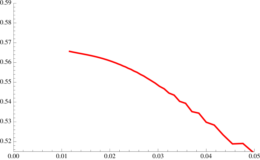
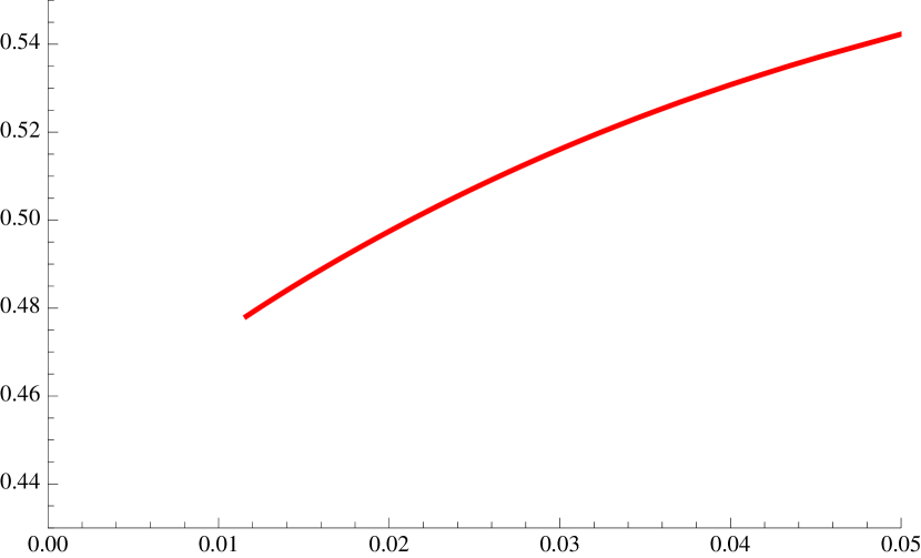
To illustrate this, we take the generating function for bridges with $u=\log 2$ as a representative value, not subject to cross-over effects present near $u=0$ and $u=\infty$. Plotting the ratios of pushed bridges against $1/n,$ as shown in Figure 1(a) gives a plot displaying considerable curvature. Note that the limiting value of $e^{\beta}$ as $n\to\infty$ is given by the top left corner of the plot. Plotting the ratios against $1/n^{2/3},$ as shown in Figure 1(b) gives a plot with reduced, but still significant, curvature. In Figures 1(c) and 1(d) we show ratio plots against $1/\sqrt{n}$ and against $1/n^{4/7}$ respectively. Both are visually linear, but more careful extrapolation reveals that plot 1(c) extrapolates, as $n\to 0,$ to a value slightly greater than the numerical value of $e^{\beta},$ while plot 1(d) extrapolates to a value indistinguishable from the numerical value of $e^{\beta}.$ Thus this simple sequence of ratio plots gives good evidence that the ratios are linear when plotted against $1/n^{\theta},$ where $0.5\leq\theta\leq 0.6,$ and is totally consistent with the heuristic expectation, $\theta=4/7=0.57142...$

Refer to caption
(a) Plot of ratios of coefficients against $\frac{1}{n}$.
Refer to caption
(b) Plot of ratios of coefficients against $\frac{1}{n^{2/3}}$.
Refer to caption
(c) Plot of ratios of coefficients against $\frac{1}{\sqrt{n}}$.
Refer to caption
(d) Plot of ratios of coefficients against $\frac{1}{n^{4/7}}$.
Figure 1: Bridge series ratios, $u=\log 2$. The top left-hand corner has ordinate $e^{\beta}$.

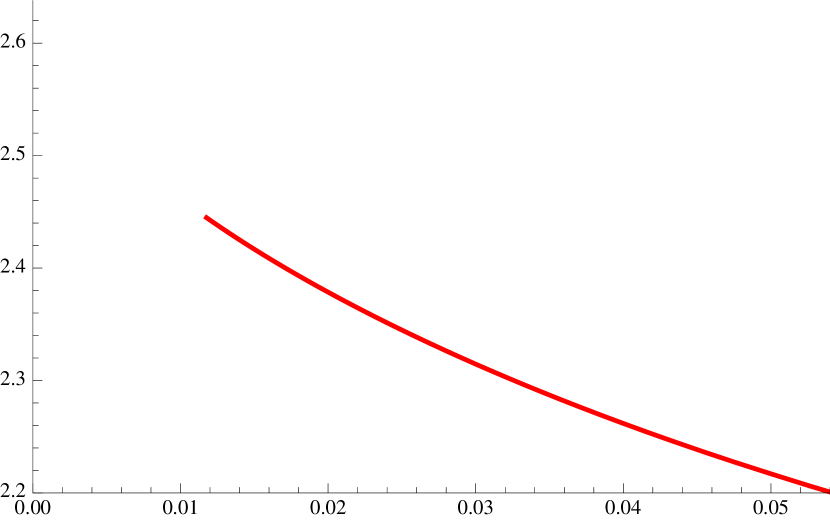
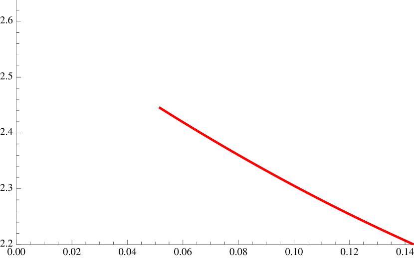
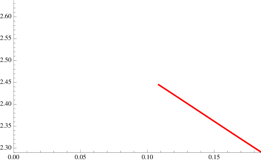
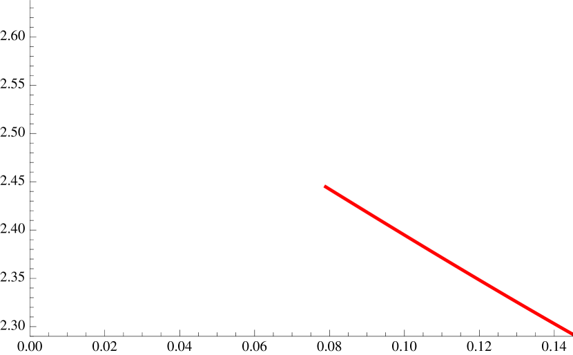
The situation is similar for pushed SAWs (figures not shown), except that for SAWs the possible range of values for $\theta,$ as chosen by visual linearity of the ratio plots, is even wider, and we estimate $0.6\leq\theta\leq 0.3,$ again consistent with the same expected value, $\theta=4/7=0.57142...$

In order to more directly estimate the value of the exponent $\sigma$, we note from (16) that

$$(r_{n}\cdot e^{-\beta}-1)\sim const\cdot n^{\sigma-1}.$$

The plot of $\log(1-r_{n}\cdot e^{-\beta})$ against $\log{n}$ should be linear, with gradient $\sigma-1.$ To the naked eye it is, so we don’t show it. However there is a small degree of curvature, so we extrapolate the local gradients, defined as

$$1-\sigma_{n}=\frac{\log\left(1-{r_{n}\cdot e^{-\beta}}\right)-\log\left(1-{r_{n-1}\cdot e^{-\beta}}\right)}{\log{(n-1)}-\log(n)},$$ (17)

against $1/n.$ The results are shown in Figure 2(a). The ordinates are estimators of $1-\sigma$, and it is clear that they are consistent with the conjectured $\sigma=3/7$.

A second estimator of $\sigma$ can be constructed from (15) by noting that

$$\log\left|\log\left(a_{n}e^{-\beta n}\right)\right|=\sigma\log{n}\left[1+O\left(\frac{\log{n}}{n^{\sigma}}\right)\right].$$

As with the previous estimator, the log-log plot of $\log\left(a_{n}e^{-\beta n}\right)$ against ${n}$ should be linear, with gradient $\sigma.$ We perform this calculation using bridges with $u=\log 2$. To the naked eye the plot is linear, so we don’t show it. As in the previous case, there is a small degree of curvature, so we again extrapolate the local ratios, as defined above mutatis mutandis, and the resulting extrapolants are shown plotted against $1/n$ in Figure 2(b). This is also entirely consistent with the expected value $3/7.$

Refer to caption
(a) Plot of estimates of $1-\sigma$ against $\frac{1}{n}$.
Refer to caption
(b) Plot of estimates of $\sigma$ against $\frac{1}{{n}}$.
Figure 2: Two different estimators of exponent $\sigma.$ Both are consistent with $\sigma=3/7=0.42857\ldots.$

We have repeated this calculation for bridges with other values of $u$, and find that this exponent estimate is numerically robust for $u$ in the range $e^{-u}\in[0.2,0.8].$ Outside this range we see crossover effects to other behaviour, as appropriate for $u=0$ and $u=\infty$. We have also repeated the calculation for SAWs with $u=\log 2$ (and other values of $u$), and find good numerical evidence for $\sigma\approx 0.43,$ supporting the expectation that $\sigma=3/7$ exactly for both models.

5.3 Estimation of $\mu_{1}.$

We now take as known the value of the exponent $\sigma,$ and, to very high precision, the value of the leading growth constant $e^{\beta}.$ We next estimate the value of the ($u$-dependent) subdominant growth constant $\mu_{1}.$ Recall that, for random walks (6), the $u$-dependence is given by

$$\log{\mu_{1}}=-\lambda_{u}=const\cdot u^{1-\sigma}.$$

(The same also occurs for compressed Dyck paths [10].) We find compelling evidence for similar $u$-dependence in the case of both pushed bridges and pushed SAWs. We also find compelling evidence that, unsurprisingly, $\mu_{1}({\rm SAWs})=\mu_{1}({\rm bridges}).$

We used several methods to estimate the value of $\mu_{1}.$ In all cases we utilised both the assumed value of the growth constant $e^{\beta}$ and the exponent $\sigma=3/7.$ No one method was especially successful for all values of $u.$ As is common with series analysis, all methods involved some sort of extrapolation. It was frequently difficult to form a view as to the limiting extrapolant in some cases, usually due to a sequence of estimates having a turning point near the end of the range. Nevertheless, by using several methods, and looking at the spread between estimates, we were able to make moderately precise estimates.

The methods we used were the following: (i) We first formed the logarithm of the ratio of successive coefficients (or, equivalently, the logarithm of the square root of the ratio of successive coefficients, $\sqrt{(}a_{n}/a_{n-2}),$ which reduces odd-even oscillations in the ratios).

$$\log\left(\frac{a_{n}}{a_{n-1}}\right)-\log{e^{\beta}}=\frac{\sigma\log{\mu_{1}}}{n^{1-\sigma}}+\frac{g}{n}+\frac{\sigma^{2}\log^{2}{\mu_{1}}}{2n^{2-2\sigma}}+O\left(n^{-2-\sigma}\right),$$

in the case of both sequences $a_{n}=b_{n}$ and $a_{n}=c^{+}_{n}$. We calculated the series expansion of the left-hand side of the above equation, known to order $n_{\rm max}=86$ in the case of bridges, and $n_{\rm max}=60$ in the case of SAWs. We fitted the terms from order $n_{\rm min}$ to order $n_{\rm max}$ to the first two, and then the first three terms in the asymptotic expansion, using the Maple procedure NonlinearFit. In each case we steadily increased the value of $n_{\rm min}$ from $(n_{\rm max}-30)$ to $(n_{\rm max}-4).$ (Attempts using the first four terms were unsuccessful, due to lack of convergence).

(ii) The second method involved directly fitting to the coefficients. Since

$$\log{a_{n}}-n\cdot{\beta}=n^{\sigma}\log{\mu_{1}}+g\log{n}+const.+O\left(n^{-\sigma}\right),$$

we could fit successive coefficient triples ($a_{k-1},\,\,a_{k}\,\,a_{k+1}$), with $k$ increasing up to $n_{\rm max}-1,$ estimating the three unknowns, $\log{\mu_{1}},\,\,g,\,\,const.$ from the three coefficients. We also fitted successive coefficient pairs ($a_{k-1},\,\,a_{k}$) to estimate the first two unknowns.

The third method (iii) used was a blend of the previous two methods, in that we fitted the logarithm of the ratio of successive coefficients to its asymptotic form by the second method – that is, a fit using successive pairs or triple of coefficients.

The next two methods, (iv) and (v) involved estimating $\mu_{1}$ directly from the ratio of successive coefficients, as given by (16). Since

$$s_{n}=r_{n}\cdot e^{-\beta}-1=\left(\frac{\sigma\log{\mu_{1}}}{n^{1-\sigma}}+\frac{g}{n}+\frac{\sigma^{2}\log^{2}\mu_{1}}{n^{2-2\sigma}}+O\left(\frac{1}{n^{2-\sigma}}\right)\right),$$

a plot of $s_{n}$ against $n^{\sigma-1}$ should be linear, with slope $\sigma\log{\mu_{1}}.$ Slight curvature was evident, so we extrapolated the local gradients.

In an attempt to get more rapid convergence, we next, (v), eliminated the term $O(1/n)$ by forming the sequence

$$t_{n}=n\cdot s_{n}-(n-1)\cdot s_{n-1}=\left(\frac{\sigma^{2}\log{\mu_{1}}}{n^{1-\sigma}}+\frac{\sigma^{2}(2\sigma-1)\log^{2}\mu_{1}}{n^{2-2\sigma}}+O\left(\frac{1}{n^{2-\sigma}}\right)\right).$$

As above, a plot of $t_{n}$ against $n^{\sigma-1}$ should be linear, with slope $\sigma^{2}\log{\mu_{1}}.$ Again, slight curvature was evident, so we again extrapolated the local gradients.

The final method, (vi), we used was based on the observation that

$$d_{n}=B_{n}(u)^{n^{-\sigma}}=\mu_{1}\left(1+\frac{g\log{n}}{n^{\sigma}}+O\left(n^{-\sigma}\right)\right),$$

so $d_{n}$ provides a sequence of estimators of $\mu_{1}$ which can be extrapolated.

We show in Table 1 the estimates of $\log{\mu_{1}}$ obtained by the six methods described. The actual analysis comprises dozens of pages, so we only give a summary. Rather than attempt to give precise error bars, which in any series analysis are perhaps better described as confidence limits, we consider it more meaningful to quote parameters to a level of precision such that we expect uncertainties to be confined to the last quoted digit. From the various estimates, we first ignore obvious outliers, then simply take the average of the remaining estimates, and give this as our combined estimate. Comparing results for SAWs and bridges, it appears that $\mu_{1}$ is the same, up to uncertainty in the quoted best estimates.

A little numerical experimentation shows that the $u$-dependence is indistinguishable from $\log\mu_{1}\propto u^{4/7}.$ We note that, like random walks (6) and Dyck paths [10], this matches $\log\mu\propto u^{1-\sigma}$. Fitting the constant of proportionality to the combined estimates leads us to the result

$$\log{\mu_{1}}\approx-2.62u^{4/7}.$$

Experimentation with data sets for other $u$-values is consistent with this result. In order to compare with the estimates given below, this formula gives $\log{\mu_{1}}=-2.913,\,\,-2.125\,\,-1.453$ for $e^{-u}=0.3,\,\,0.5,\,\,0.7$ respectively.

Method $e^{-u}=0.3$ $e^{-u}=0.5$ $e^{-u}=0.7$
(i) Bridges, 2 terms $>-2.98$ $\approx-2.177$ $>-1.51$
(i) Bridges, 3 terms $\approx-2.89$ $>-2.180$ $<-1.30$
(ii) Bridges, 2 terms $-3.0$ $-2.15$ $-1.5$
(ii) Bridges, 3 terms $-2.92$ $n.c.$ $-1.46$
(iii) Bridges, 2 terms $-2.905$ $-2.13$ $-1.47$
(iii) Bridges, 3 terms $n.c.$ $n.c.$ $-1.46$
(iv) Bridges $-2.96$ $-2.14$ $-1.47$
(v) Bridges $-2.92$ $-2.14$ $n.c.$
(vi) Bridges $-3.0$ $-2.21$ $-1.5$
Combined Estimate -2.92 -2.14 -1.465
(i) SAWs, 2 terms $>-3.00$ $>-2.21$ $>-1.55$
(i) SAWs, 3 terms n.c. $\approx-2.14$ $>-1.485$
(ii) SAWs, 2 terms $>-2.98$ $-2.13$ $-1.5$
(ii) SAWs, 3 terms $\leq-2.90.$ $n.c.$ $-1.45$
(iii) SAWs, 2 terms $-2.87$ $-2.135$ $-1.47$
(iii) SAWs, 3 terms $-2.92.$ $n.c.$ $-1.45$
(iv) SAWs $-2.84$ $-2.12$ $-1.42$
(v) SAWs $-2.89$ $-2.15$ $-1.47$
(vi) SAWs $n.c.$ $n.c$ $n.c.$
Combined Estimate -2.91 -2.13 -1.45
Table 1: Estimates of $\log{\mu_{1}}$ for SAWs and bridges for various $e^{-u}$ values, using the six methods described. ($n.c.$ means no convergence).

5.4 Estimation of the exponent $g.$

In the previous section we estimated the value of $\mu_{1}$ from the series assuming the values of $e^{\beta}$ and $\sigma.$ Attempting to do the same in order to estimate the exponent characterising the sub-sub-dominant term $n^{g}$ making the same assumptions was unsuccessful. That is to say, we could not come up with any method of analysis that gave a consistent estimate of $g$ for the SAW or bridge case. Note that we expect $g$ to be $u$-independent, but not necessarily to be the same for SAWs and bridges.

However if we accept the conjecture (above) that $\mu_{1}({\rm SAWs})=\mu_{1}({\rm bridges}),$ one can estimate $g_{\rm SAWs}-g_{\rm bridges}$ by studying the asymptotics of the series formed by taking the term by term quotient of the SAW and the bridge series. Defining $v_{n}=c^{+}_{n}/b_{n},$ we expect from the asymptotics that $v_{n}\sim const\cdot n^{\alpha},$ where $\alpha=g_{\rm SAWs}-g_{\rm bridges}.$

For $e^{-u}$ in the range $[0.1,0.6]$ we find estimates of $\alpha,$ obtained by calculating the gradient of a simple ratio plot of $r_{v}(n)=v_{n}/v_{n-1}$ against $1/n$, to lie consistently in the range $0.61$ to $0.63.$ For $e^{-u}\geq 0.7$ the exponent estimators clearly have a turning point at a value beyond the number of coefficients we have available. Accordingly, we cannot estimate $\alpha$ in this $u$-regime.

In order to estimate the individual exponents, we re-analyse the original series using not only our best estimate of $e^{\beta}$ and the value $\sigma=3/7,$ but also the estimate of $\mu_{1}$ obtained in the previous section. We can, using these values, divide the original series coefficients by $e^{n\beta}\cdot\mu_{1}(u)^{n^{\sigma}}.$ The resultant coefficients should behave asymptotically as $const\cdot n^{g}.$ Thus $g$ can be estimated in a variety of ways, but given the uncertainty in the value of $\mu_{1},$ there is no point in using sophisticated methods. Rather, we just look at the gradient of the ratio plot of the divided coefficents, when plotted against $1/n.$ The ratio of succesive coefficients in this case should behave as $1+g/n+o(g/n)$. Thus plotting the ratios against $1/n$ should give a straight line with gradient $g$.

In this way we estimate $g_{\rm SAWs}\approx 0.15,\,\,0.15,\,\,0.16$ for $e^{-u}=0.3,\,\,0.5,\,\,0.7$ respectively, and $g_{\rm bridges}\approx-0.5,\,\,-0.5,\,\,-0.44$ for $e^{-u}=0.3,\,\,0.5,\,\,0.7$ respectively. These results are reasonably consistent with the preceding estimate that the gap between the exponents should be in the range $0.61$ to $0.63.$ Our estimate for $g_{\rm bridges}$ has an uncertainty of about $\pm 0.05,$ while that of $g_{\rm SAWs}$ is $\pm 0.02$, so our estimates have a difference of $0.65\pm 0.07,$ which is reasonably consistent with the direct estimate found above.

The heuristic arguments in the previous section predict that $g_{\rm bridges}=-\frac{13}{28}=-0.4642857\ldots,$ in agreement with our analysis above, while $g_{\rm SAWs}=\frac{3}{16}=0.18750,$ again in agreement with the above analysis. Similarly, $\alpha=\frac{73}{112}=0.651785\ldots,$ as against our direct estimates of $\alpha\approx 0.65$ and $\alpha\approx 0.62.$

6 Conclusion

We have studied several models of self-avoiding walks (SAWs) and polygons (SAPs) which are constrained to lie in the upper half-plane and are subjected to a compressive force. The force is applied to the vertex or vertices of the walk located at the maximum distance above the boundary of the half-space. We have in particular focused on three types of objects: SAWs, SAPs and self-avoiding bridges. In each case, we have considered the partition function of objects of size $n$, with the aim of determining the asymptotic behaviour of these partition functions in the $n\to\infty$ limit.

We used the conjectured relation with the Schramm-Loewner evolution to predict the asymptotic forms of the partition functions, including the values of the exponents. These values, as stated in Prediction 2, are that (for SAWs, bridges and SAPs respectively)

$\displaystyle C^{\rm max}_{n}(u)$ $\displaystyle\sim A^{+}_{u}\,n^{3/16}\,\exp\{-\lambda_{1}u^{4/7}\,n^{3/7}\},$
$\displaystyle B_{n}(u)$ $\displaystyle\sim A^{b}_{u}\,n^{-13/28}\,\exp\{-\lambda_{1}u^{4/7}\,n^{3/7}\},$
$\displaystyle P^{\rm max}_{n}(u)$ $\displaystyle\sim A^{p+}_{u}\,n^{-11/7}\,\exp\{-\lambda_{2}u^{4/7}\,n^{3/7}\},$

where $u>0$ corresponds to the compressive force regime, $\lambda_{1},\lambda_{2}>0$ are constants and $A^{+}_{u},A^{b}_{u},A^{p+}_{u}$ are functions of $u$.

Finally, we tested the predictions for SAWs and bridges by analysing exact enumeration data and found them to be in agreement (within the range of uncertainty resulting from analysis of limited series data). A similar analysis for SAPs has been performed elsewhere.

Acknowledgements

This work was supported by an award (IJ) under the Merit Allocation Scheme on the NCI National Facility at the ANU and by funding under the Australian Research Council’s Discovery Projects scheme by the grant DP140101110 (AJG and IJ). Gregory Lawler is supported by National Science Foundation grant DMS-0907143. Nicholas Beaton is supported by the Pacific Institute for the Mathematical Sciences.

References

  • [1] R Bauerschmidt, D C Brydges and G Slade, Logarithmic correction for the susceptibility of the 4-dimensional weakly self-avoiding walk: a renormalisation group analysis, Preprint, available at http://arxiv.org/abs/1403.7422, 2014.
  • [2] N R Beaton, The critical pulling force for self-avoiding walks, Journal of Physics A: Mathematical and Theoretical 48 (2015), 16FT03.
  • [3] N Clisby, Accurate estimate for the critical exponent $\gamma$ for self-avoiding walks via a fast implementation of the pivot algorithm, preprint.
  • [4] N Clisby, Accurate estimate of the critical exponent $\nu$ for self-avoiding walks via a fast implementation of the pivot algorithm, Physical Review Letters 104 (2010), 055702.
  • [5] N Clisby and I Jensen, A new transfer-matrix algorithm for exact enumerations: self-avoiding polygons on the square lattice, Journal of Physics A: Mathematical and Theoretical 45 (2012), 115202+.
  • [6] A R Conway, I G Enting, and A J Guttmann, Algebraic techniques for enumerating self-avoiding walks on the square lattice, Journal of Physics A: Mathematical and General 26 (1993), 1519–1534.
  • [7] H Duminil-Copin and S Smirnov, The connective constant of the honeycomb lattice equals $\sqrt{2+\sqrt{2}}$, Annals of Mathematics 175 (2012), 1653–1665.
  • [8] I G Enting, Generating functions for enumerating self-avoiding rings on the square lattice, Journal of Physics A: Mathematical and General 13 (1980), 3713–3722.
  • [9] P J Flory, The configuration of real polymer chains, Journal of Chemical Physics 17 (1949), 303–310.
  • [10] A J Guttmann, Analysis of series expansions for non-algebraic singularities, Preprint, available at http://arxiv.org/abs/1405.5327, 2014.
  • [11] A J Guttmann, I Jensen and S G Whittington, Pulling adsorbed self-avoiding walks from a surface, Journal of Physics A: Mathematical and Theoretical 47 (2014), 015004.
  • [12] A J Guttmann, I Jensen and S G Whittington, Polygons pulled from an adsorbing surface, In preparation.
  • [13] J M Hammersley, Percolation processes II. The connective constant, Mathematical Proceedings of the Cambridge Philosophical Society 53 (1957), 642–645.
  • [14] T Hara and G Slade, Self-avoiding walk in five or more dimensions I. The critical behaviour, Communications in Mathematical Physics 147 (1992), 101–136.
  • [15] E J Janse van Rensburg and S G Whittington, Adsorbed self-avoiding walks subject to a force, Journal of Physics A: Mathematical and Theoretical 46 (2013), 435003+.
  • [16] I Jensen, Enumeration of self-avoiding walks on the square lattice, Journal of Physics A: Mathematical and General 37 (2004), 5503–5524.
  • [17] I Jensen, A new transfer-matrix algorithm for exact enumerations: self-avoiding walks on the square lattice, Preprint, available at http://arxiv.org/abs/1309.6709, 2013.
  • [18] T Kennedy and G Lawler, Lattice effects in the scaling limit of the two-dimensional self-avoiding walk, AMS Contemporary Mathematics 601 (2013), 195– 210.
  • [19] J Krawczyk, A L Owczarek, T Prellberg and A Rechnitzer, Pulling adsorbing and collapsing polymers from a surface, Journal of Statistical Mechanics: Theory and Experiment 2005 (2005), P05008+.
  • [20] G Lawler, Cut points for simple random walk, Electronic Journal of Probability 1 (1996), paper #13.
  • [21] G Lawler and W Werner, Universality for conformally invariant intersection exponents, J. European Math. Soc. 2 (2000), 291–328.
  • [22] G Lawler, O Schramm, and W Werner, Values of Brownian intersection exponents II: plane exponents, Acta Math. 187 (2001), 275-308.
  • [23] G Lawler, O Schramm and W Werner, Conformal restriction: The chordal case, J. Amer. Math. Soc. 16 (2003), 917–955.
  • [24] G Lawler, O Schramm and W Werner, On the scaling limit of planar self-avoiding walk, in Proceedings of the Conference on Fractal Geometry and Applications: A Jubilee of Benoit Mandelbrot, M. Lapidus and M. van Frankenhuijsen, Vol. 2, ed., Amer. Math. Soc. (2004), 339–364.
  • [25] G Lawler and S Sheffield, A natural parametrization for the Schramm-Loewner evolution, Annals of Probab. 39 (2011), 1896– 1937.
  • [26] G Lawler and M Rezaei, Minkowski content and natural parameterization for the Schramm-Loewner evolution, to appear in Annals of Probability.
  • [27] B Nienhuis, Exact critical point and critical exponents of O(n) models in two dimensions, Physical Review Letters 49 (1982), 1062–1065.
  • [28] W J C Orr, Statistical treatment of polymer solutions at infinite dilution, Transactions of the Faraday Society 43 (1947), 12–27.
  • [29] O Schramm, Scaling limits of loop-erased random walk and uniform spanning trees, Israel J. Math. 118 (2000), 221-288.
  • [30] A M Skvortsov, L I Klushin, A A Polotsky, and K Binder, Mechanical desorption of a single chain: Unusual aspects of phase coexistence at a first-order transition, Physical Review E 85 (2012), 031803.
  • [31] W Zhang and X Zhang, Single molecule mechanochemistry of macromolecules, Progress in Polymer Science 28 (2003), 1271–1295.

Appendix A Asymptotics of an integral

Several times in this paper, we used the asymptotics of a particular integral. Here we justify that relation.

Lemma 1.

If $\alpha,b,k>0,r\in{\mathbb{R}}$, then as $m\rightarrow\infty$,

$$\int_{0}^{\infty}y^{r}\,\exp\left\{-\left(\frac{km}{\alpha(by)^{\alpha}}+by\right)\right\}\,dy\sim C\,m^{\frac{2r+1}{2(1+\alpha)}}\,\exp\left\{-\lambda\,m^{\frac{1}{1+\alpha}}\right\},$$ (18)

where

$$C=\,b^{-(1+r)}\,k^{\frac{2r+1}{2(1+\alpha)}}\sqrt{\frac{2\pi}{1+\alpha}},\qquad\lambda=\frac{(\alpha+1)\,k^{\frac{1}{1+\alpha}}}{\alpha}=\frac{(\alpha+1)}{\alpha}\,\left(\frac{k}{b^{\alpha}}\right)^{\frac{1}{1+\alpha}}\,b^{\frac{\alpha}{1+\alpha}}.$$
Proof.

Using the change of variables $x=by$, we see it suffices to prove the result for $b=1$. We write $km=n^{1+\alpha}$, so it suffices to show that

$$\int_{0}^{\infty}x^{r}\,\exp\left\{-\left(\frac{n^{1+\alpha}}{\alpha x^{\alpha}}+x\right)\right\}\,dx=\sqrt{\frac{2\pi}{1+\alpha}}\,n^{r+\frac{1}{2}}\,e^{-n(\frac{\alpha+1}{\alpha})}\,\left[1+O(n^{-1/2})\right].$$

Using the substitution $x=n^{1/2}y+n$,

$\displaystyle\int_{0}^{\infty}x^{r}\,\exp\left\{-\left(\frac{n^{1+\alpha}}{\alpha x^{\alpha}}+x\right)\right\}\,dx$
$\displaystyle=$ $\displaystyle n^{r+\frac{1}{2}}\int_{-\sqrt{n}}^{\infty}\left(1+\frac{y}{\sqrt{n}}\right)^{r}\exp\left\{-n\,\left(\frac{n^{\alpha}}{\alpha(n^{1/2}y+n)^{\alpha}}+\frac{y}{\sqrt{n}}+1\right)\right\}\,dy$
$\displaystyle=$ $\displaystyle n^{r+\frac{1}{2}}\,e^{-n(1+\frac{1}{\alpha})}\int_{-\sqrt{n}}^{\infty}\left(1+(y/\sqrt{n})\right)^{r}\,\exp\left\{-n\,g(y/\sqrt{n})\ \right\}\,dy,$

where

$$g(t)=g_{\alpha}(t)=\alpha^{-1}\left((t+1)^{-\alpha}-1\right)+t.$$

Using the substitution $t=y/\sqrt{n}$,

$$n^{-(r+\frac{1}{2})}\,e^{n(1+\frac{1}{\alpha})}\int_{0}^{\infty}x^{r}\,\exp\left\{-\left(\frac{n^{1+\alpha}}{\alpha x^{\alpha}}+x\right)\right\}\,dx=\sqrt{n}\,\int_{-1}^{\infty}(1+t)^{r}\,\exp\left\{-n\,g(t)\right\}\,dt.$$

Since $g(0)=0,g^{\prime}(0)=0,g^{\prime\prime}(0)=\alpha+1$, we have

$$g(t)=\frac{\alpha+1}{2}\,t^{2}+O(t^{3}),$$

which is valid for $|t|\leq 1/2$. Note that there exists $c>0$ such that

$$g(t)\geq c\,n^{-2/3},\;\;\;\ |t|\geq n^{-1/3},$$
$$g(t)\geq t-\alpha^{-1}\;\;\;\;t\geq 0,$$
$$g(t)\geq\frac{1}{(1+t)^{\alpha}}-\frac{\alpha+1}{\alpha},\;\;\;\;-1<t\leq-\frac{1}{2}.$$

Using these estimates in order, we see that

$$\int_{-1+n^{-1}}^{2/\alpha}(1+t)^{r}\exp\{-ng(t)\}\,\mathbbm{1}_{\{|t|\geq n^{-1/3}\}}\,dt=O\left(n^{|r|}\,\exp\left\{-cn^{1/3}\right\}\right)=o(n^{-1/2}),$$
$$\int_{2/\alpha}^{\infty}(1+t)^{r}\exp\{-ng(t)\}\,dt\leq e^{n/\alpha}\,\int_{2/\alpha}^{\infty}(1+t)^{r}\exp\{-nt\}\,dt\leq O(n^{|r|}\,e^{-n/\alpha})=o(n^{-1/2}),$$
$$\int_{-1}^{-1+n^{-1}}(1+t)^{r}\exp\{-ng(t)\}\,dt=o(n^{-1/2}).$$

Hence,

$$\sqrt{n}\,\int_{-1}^{\infty}(1+t)^{r}\,\exp\left\{-n\,g(t)\right\}\,dt=o(n^{-1/2})+\sqrt{n}\,\int_{-n^{-1/3}}^{n^{-1/3}}(1+t)^{r}\,\exp\left\{-n\,g(t)\right\}\,dt.$$

For $|t|\leq n^{-1/3}$, we write

$\displaystyle(1+t)^{r}\,e^{-ng(t)}$ $\displaystyle=[1+O(t)]\,\exp\left\{-n\left(\frac{\alpha+1}{2}\,t^{2}+O(t^{3})\right)\right\}$
$\displaystyle=e^{-n(\alpha+1)t^{2}/2}\,[1+O(t)+O(nt^{3})].$

Here we have restricted to $|t|\leq n^{-1/3}$ so that $nt^{3}=O(1)$ and hence the expansion $e^{O(nt^{3})}=1+O(nt^{3})$ is valid.

Then

$$\sqrt{n}\,\int_{-n^{-1/3}}^{n^{-1/3}}e^{-n(\alpha+1)t^{2}/2}\,dt=\int_{-n^{1/6}}^{n^{1/6}}e^{-(\alpha+1)s^{2}/2}\,ds=\sqrt{\frac{2\pi}{(\alpha+1)}}-o(n^{-1/2}),$$

and

$$\sqrt{n}\,\int_{-n^{-1/3}}^{n^{-1/3}}\left(|t|+n|t|^{3}\right)\,e^{-n(\alpha+1)t^{2}/2}\,dt\leq\int_{-\infty}^{\infty}\frac{|s|+|s|^{3}}{\sqrt{n}}\,e^{-(\alpha+1)s^{2}/2}\,ds=O(n^{-1/2}).$$