Principal Component Analysis of computed emission lines from proto-stellar jets

Abstract

A very important issue concerning protostellar jets is the mechanism behind their formation. Obtaining information on the region at the base of a jet can shed light into the subject and some years ago this has been done through a search for a rotational signature at the jet line spectrum. The existence of such signatures, however, remains controversial. In order to contribute to the clarification of this issue, in this paper we show that the Principal Component Analysis (PCA) can potentially help to distinguish between rotation and precession effects in protostellar jet images. This method reduces the dimensions of the data, facilitating the efficient extraction of information from large datasets as those arising from Integral Field Spectroscopy. The PCA transforms the system of correlated coordinates into a system of uncorrelated coordinates, the eigenvectors, ordered by principal components of decreasing variance. The projection of the data on these coordinates produces images called tomograms, while eigenvectors can be displayed as eigenspectra. The combined analysis of both can allow the identification of patterns correlated to a particular physical property that would otherwise remain hidden, and can help separating in the data the effect of physically uncorrelated phenomena. These are for example, rotation and precession in the kinematics of a stellar jet. In order to show the potential of the PCA analysis, we apply it to synthetic spectro-imaging datacubes generated as an output of numerical simulations of protostellar jets. In this way we generate a benchmark to which a PCA diagnostics of real observations can be confronted. Using the computed emission line profiles for [O I]$\lambda$6300 and [S II]$\lambda$6716, we recover and analyze the effects of rotation and precession in tomograms generated by PCA. We show that different combinations of the eigenvectors can be used to enhance and to identify the rotation features present in the data. Our results indicate that the PCA can be useful for disentangling rotation from precession in jets with an inclination of the jet with respect to the plane of the sky as high as $45^{\circ}$. We have been able to recover the initially imposed rotation jet profile for models at moderate inclination angle ($\phi\leq 15^{\circ}$) and without precession.

1. Introduction

Recent observations of protostellar jets show, in some cases, a systematic side-to-side (with respect to the jet axis) shift in radial velocities in several emission lines in the optical and UV. Davis et al. (2000) and Bacciotti et al. (2002) reported the first results of this kind, in a molecular and atomic jet, respectively. In particular, Bacciotti et al. (2002) presented an analysis performed on high resolution Hubble Space Telescope (HST) long-slit spectra taken at different positions, both along and across the DG Tau jet, in the region close to its driving source. They found a systematic side-to-side difference in the radial velocity of the jet with respect to its axis, which they interpreted as evidence of jet rotation, what was later found to be in agreement with the sense of rotation of the circumstellar disk of DG Tau (Testi et al., 2002).

This observational finding has been followed by other studies which tried to look for the same kind of pattern in other jet sources. Coffey et al. (2004), using the Space Telescope Imaging Spectrograph (STIS) of the HST found similar results for the jets in the T Tauri stars TH 28, RW Aur and LkH$\alpha$ 321. Consistently with the predictions of the magnetocentrifugally driven mechanism for jet launching (e.g., Blandford & Payne, 1982; Ferreira, 1997), the bipolar collimated outflows in TH 28 and RW Aur showed the same signs of velocity asymmetry in both red- and blue-shift lobes, implying the same sense of rotation in both. However, the sense of the jet rotation in RW Aur was later inferred to be the opposite of the disk rotation (Cabrit et al., 2006). Furthermore, recent observations by Coffey et al. (2012) showed a radial velocity shift of order of $\sim 10$ km/s in the near-UV, corresponding to a rotation in the opposite sense of that determined by the optical observation. In addition, no shift in velocity was detected in the observation of RW Aur with the same instrument six months later (Coffey et al., 2012).

The CW Tau and HH 30 jets were observed in the near ultraviolet (NUV) and optical wavelengths, using STIS by Coffey et al. (2007), who also presented new observations of the DG Tau and TH 28 jets. A systematic radial velocity shift pattern was observed in the CW Tau jet spectra in the same range of velocities, of $\sim 10-20$ km s^-1 for the optical shifts, with slightly smaller shifts in the NUV ($\sim 5-10$ km s^-1), while no significant shift in radial velocity was observed for the HH 30 jet. For this jet, Pety et al. (2006) did not observe also any rotation signature at millimeter wavelengths. As noted by, e.g., Cai et al. (2008), the lack of any rotational evidence for HH 30 jet is unexpected since the rotation signature should be maximum for jets moving in the plane of the sky as is the case of HH 30 (inclination angle $\lesssim 1^{\circ}$, Mundt et al. 1990).

These optical and NUV observations of a sample of jets have been followed by near-infrared (NIR) long slit spectroscopy of HH 212 carried out by Correia et al. (2009). HH 212 is one of the bona fide examples of jet symmetry (between both lobes) and the first HH jet for which evidence of rotation was found (Davis et al., 2000). In their work, Correia et al. (2009) argued that the combined effect of rotation and precession of the jet axis would be responsible for the observed pattern, and that rotation alone would not be able to account for the data. The HH 212 jet has also been observed by Codella et al. (2007), who did not find evidence of velocity gradients compatible with rotation in SiO observations.

Along with these efforts, attempts have been made to observe rotation of the jet axis through ground based, world class telescopes. Coffey et al. (2011) used the Gemini South Telescope to observe HH 34, HH 111 and HH 212. They found evidences for rotation in some knots of HH 111 and 212. For HH 111, they noted that the sense of rotation obtained for the observed knot is in opposite sense to the disk rotation, while for HH 212 they agree (in both receding and approaching lobes, and the disk itself). Coffey et al. (2015) looked for radial velocity shifts in the RY Tau system, by using Gemini NIFIS+ALTAIR observations of the jet, combined with radio observations of the disk using the Plateau de Bure. Although a Keplerian rotation pattern for the disk was clearly obtained, the value of the radial velocity shifts remained below the 3$\sigma$ detection limit. However, the authors considered the obtained radial velocity values as upper limits and assuming steady state, constrained the launching region to be below 0.45 AU. In Fendt (2011) a comprehensive list and a detailed discussion of HH objects for which there is evidence for jet rotation are presented.

If the rotation interpretation is correct, these studies open an important new window to investigate the physics behind the jet production and launching mechanisms. The measurement of jet rotation has implications in the estimate of the angular momentum flux lost by the system, on the determination of the footpoints of the jet launching region, and could help to discriminate among different jet production models (see, for instance, Pudritz 2004). The comparison between the expected values for the radial velocity asymmetry, from magnetohydrodynamics (MHD) disk wind models, and the values obtained for DG Tau by Bacciotti et al. (2002) was presented by Pesenti et al. (2004). They found that both classes of MHD disk wind models, the so-called cold and warm solutions (see Casse & Ferreira, 2000a, b), are able to adjust the observed trend for DG Tau transverse radial velocity, but only the warm solution is able to reproduce the velocity shifts.

The indication of rotation in DG Tau, TH 28 and LkH$\alpha$128 is also consistent with a wind launched at the innermost part of the accretion disk. It also reproduces the onion like structure (in radial velocities) expected for a wind launched by an accretion disk. Anderson et al. (2003) found for the DG Tau jet, using Bacciotti et al. (2002) data, a launching radius of $r_{0}\sim 0.3-4$ AU from the YSO, thus excluding the X-wind model (e.g., Cai et al., 2008) as a jet launching mechanism. The observational determination of the launching region is, unarguably, a key piece to advance further and to gather all the information in a consistent and complete model.

However, the interpretation of side-to-side velocity shifts as evidence of rotation is still controversial. Side to side asymmetries in the velocity along the main jet axis of order of 10% of the observed jet speed would produce an effect on the radial velocity similar to that observed in the works cited above. In this sense, the lack of velocity shifts in HH 30 and the presence of clear side-to-side asymmetries in the electron and hydrogen densities of some of the jets where the radial velocity shifts are measured (e.g., Th28, see Coffey, Bacciotti & Podio 2008) are consistent with the possibility that at least part of the observed radial velocity shifts originates from side-to-side asymmetries in the velocity of the jet along the direction of the jet propagation.

Cerqueira et al. (2006) discussed the possibility that the precession of the jet axis could also give rise to the same radial velocity asymmetries observed on jet spectra by, for example, Bacciotti et al. (2002). They also investigated the combined effect of precession and rotation, which seem to operate together in the DG Tau jet. While it is clear that the models presented by Cerqueira et al. (2006) do not apply for jets with small ($\lesssim 5^{\circ}$) precession angles, as mentioned by Coffey et al. (2007), it is also evident that at least for those systems that show evidence for precession (e.g., DG Tau), its presence should be considered properly.

We propose here a method that could be used to distinguish between rotation and precession and in general any asymmetry in the velocity components of the jet when interpreting a given spectra from a Fabry-Perot or an Integral Field Unit (IFU)-like data. For this purpose, we perform a Principal Component Analysis (PCA) of synthetic spectra generated from the numerical simulations performed in Cerqueira et al. (2006), intended here as idealized reproductions of the observations. Following this approach, we construct 3D synthetic datacubes in two relevant emission lines ([S II]$\lambda$6716   and [O I]$\lambda$6300) and then apply the PCA technique to split the spectra into its components ranked by the variance. The main goal of this work is to show how the PCA can help disentangling the different mechanisms that cause asymmetries at the jet lines for rotating and precessing jets.

The paper is organized as follows. In Section 2 we discuss the PCA technique as applied in our numerical simulations, which are briefly reviewed in Section 3. In Section 4 we discuss tomograms and eigenspectra and their physical interpretation. In Section 5 the results based on the reconstructed process of the treated datacube are shown and in Section 6 the main conclusions are presented. In the Appendix A we present Tables for eigenvalues and in the Appendix B we show how the analysis change when we take into account noisy data and how we can extract the desired information through the use of the enhancement factor in PCA.

2. The PCA technique applied to a datacube

The Principal Component Analysis (PCA) is a method to extract information from large, multidimensional datasets, to identify peculiar patterns in the data that would otherwise remain hidden or mutually combined. The isolated patterns can in many cases be associated to physical properties that would remain undetected in traditional spectro-imaging diagnostics. This is done through the construction of a new system of “natural” uncorrelated coordinates ordered by decreasing variance with respect to the average image/spectrum. This new system describes the dataset in a more efficient way, as the projection of the data on each coordinate isolates one relevant information.

In the presentation of the PCA technique, we will use the same formalism of Steiner et al. (2009), Ricci et al. (2011) and Menezes et al. (2014). These authors developed a PCA-based tool to investigate the properties of datacubes obtained from observations made with the Gemini Multi-Object Spectrograph in its Integral Field Unit mode (GMOS-IFU) for active galaxies (NGC 4736, NGC 7097 and NGC 3115, respectively). First, they use PCA, together with other cleaning techniques, to remove instrumental spatial fingerprints (see also Cerqueira et al. 2015, who applied the same cleaning technique to GMOS-IFU observations of the HH 111 jet). As we shall see below, in the PCA technique a given datacube is firstly reduced to a particular bi-dimensional array from which one calculates the covariance matrix. Eigenvectors and eigenvalues are then determined for this matrix, and ordered by decreasing variance. The eigenvectors constitute the new orthogonal basis, and the data can be projected on this basis to form the tomograms. Each tomogram will highlight a particular pattern in the data. The tomograms, that are bi-dimensional maps which describe the data in an orthogonal basis of uncorrelated coordinates, can then be interpreted and can reveal physical properties associated with the obtained pattern. Tomograms can be combined linearly to reconstruct cleaned 2D images in the normal space in which that particular property is now evident.

2.1. Preparing the data for the PCA analysis

In the more general case, we simulate a jet that can precess and rotate (see Figure 1). The axis of precession makes an angle $\phi$ with respect to the plane of the sky, assumed here to be the (x,y) plane. The axis of the rotating/precessing jet lies along a cone that makes an angle $\theta$ with respect to the axis of precession. A non precessing, but rotating jet has $\theta=0$. We compute as an output of the numerical simulation the flux of each emission line arranged in a tridimensional datacube with two spatial and one spectral dimensions. Each element of the datacube collects the flux produced in a square region of 5.74 AU (the spatial resolution of the simulation) in (x,y), in the radial velocity interval from -400 km s^-1 to +100 km s^-1 (corresponding to a spectral width of $\sim 10$ Å  for [O I]$\lambda$6300 and $\sim 11$ Å  for [S II]$\lambda$6716), with a spectral sampling of 10 km s^-1. The datacube will have $n=\mu\times\nu$ = 128$\times$128 pixels in space and $m$ = 50 pixels in wavelength. Our data is equivalent to those generated by an IFU: from the simulation, we can obtain velocity channel maps around a given emission line for a fixed wavelength. By varying the wavelength, we obtain a datacube (see Cerqueira et al., 2006).

For each value of $m$ we can define an intensity, $(\mathrm{I}_{ij\lambda})_{0}$, with $i=1,\dots,\mu$; $j=1,\dots,\nu$; $\lambda=1,\dots,m$. The “0” index refers to the original intensity extracted from the data (see Ricci et al. 2011 and Steiner et al. 2009), i.e., the original intensity at each velocity channel map. Since ${\mu}$ and $\nu$ are the total number of pixels in the $x$ and $y$ spatial directions we can define the average spectrum of the datacube as the intensity averaged over the two spatial dimensions:

$$Q_{\lambda}=\frac{1}{n}\sum_{i=1}^{\mu}\sum_{j=1}^{\nu}(I_{ij\lambda})_{0}\;,$$ (1)

where $n=\mu\times\nu$. This mean emission is used to redefine the datacube as:

$$I_{ij\lambda}=(I_{ij\lambda})_{0}-Q_{\lambda}\;,$$ (2)

which is the excess (or deficit) of flux in comparison to the average flux at each pixel at a given wavelength.

Since we are looking for patterns of variation in the data, the subtraction of the average spectra is an important procedure. As pointed out by Steiner et al. (2009), this also eliminates components of emission in the spectra that have null spatial variance at a given wavelength, as is the case of the sky emission that could be eventually constant in the observed field in real (i.e., not synthetic) datacubes.

We can now transform the datacube in an intensity matrix, ${\bf I}_{\beta\lambda}$, of $n$ rows (the spatial pixels) and $m$ columns (the spectral pixels). The spatial pixel in the intensity matrix ($\beta$) is related to the datacube spatial pixels ($i$ and $j$) through the relation

$$\beta=\mu(i-1)+j\,{\rm.}$$ (3)

This univocal relation is used to i) build up the intensity matrix (${\bf I}_{\beta\lambda}$) mentioned before and ii) to recover the datacube intensity for a given projection (see Section §2.2 below), which can contain the whole data or just a fraction of it. In the simulations that we are going to present in this paper, $\mu=\nu=128$ and $m=50$ (and so $n=16\,384$).

The matrix ${\bf I}_{\beta\lambda}$ is then ready to be processed using the PCA technique. In the next section we discuss the PCA pipeline as described in Steiner et al. (2009). We present here the same approach but for simulated datacubes. Our aim, as already emphasized, is to use controlled inputs, including different physical mechanisms like precession and rotation, to see their imprints in the tomograms. Here, we want to test the potential of PCA in disentangling the effects of rotation and precession in real data of protostellar jets.

2.2. An orthogonal basis of uncorrelated coordinates

The main goal of the PCA technique is to represent the data in a new set of mutually orthogonal basis formed finding the eigenvectors and eigenvalues of the covariance matrix of the modified dataset ${\bf I}_{\beta\lambda}$, defined as:

$${\bf C}_{\rm{cov}}=\frac{[{\bf I}_{\beta\lambda}]^{\rm T}\cdot{\bf I}_{\beta\lambda}}{n-1}\,{\rm,}$$ (4)

(see Steiner et al., 2009) where $[{\bf I}_{\beta\lambda}]^{\rm T}$ is the transpose of the intensity matrix, ${\bf I}_{\beta\lambda}$. The covariance matrix has $m$ eigenvalues, representing the variance of the data for the associated eigenvector $E_{k}$ (where $k$ is the order of the eigenvector), that can be ranked in the new basis with decreasing value of the variance, i.e. from the largest ($\Lambda_{1}$) to the smallest ($\Lambda_{m}$) variance, as just the ones corresponding to the largest variances will contain relevant information. The variances can be represented in a normalized way in terms of percentages, and they are the diagonal elements of the covariance matrix; the sum of all variances must return $\sum_{k=1}^{m}\Lambda_{k}=1$ (or 100%).

The eigenvectors represent a new orthogonal basis in which the data can be described. These eigenvectors are used to build the characteristic matrix, ${\bf E}_{\lambda k}$, which has $m$ eigenvectors in its columns, sorted by decreasing variance. In this new orthogonal basis, the data can be decomposed as:

$${\bf T}_{\beta k}={\bf I}_{\beta\lambda}\cdot{\bf E}_{\lambda k}\,,$$ (5)

where ${\bf T}_{\beta k}$ is the intensity matrix expressed in the new basis. In this basis, the covariance matrix ${\bf D}_{\rm{cov}}$, defined as:

$${\bf D}_{\rm{cov}}=\frac{[{\bf T}_{\beta k}]^{\rm T}\cdot{\bf T}_{\beta k}}{n-1}\,{\rm,}$$ (6)

is diagonal by construction (orthogonality property), which means that it has null covariance between different coordinates and its diagonal elements are the eigenvalues. Since the basis is orthogonal, the projection ${\bf T}_{\beta k}$ on the space of eigenvectors represents a pattern that is uncorrelated for each $k$, and one can refer to uncorrelated physical properties that can be separated and recognized.

A way to visualize the projection ${\bf T}_{\beta k}$ of the data onto the new basis is to produce from it 2D images called tomograms. The tomogram is the quantity ${\bf T}_{i,j,k}$ obtained by ${\bf T}_{\beta k}$ by selecting a given $k=k^{\prime}$ and by unpacking $\beta$ into the two indexes $i,j$ by inverting equation (3). It is important to emphasize that the tomograms are images of the 3D data in the new system of coordinate. As in Steiner et al. (2009), the tomogram for the $k-$eigenvector is an image that arises when we use equations (3) and (5) for a given $k$, to assign a value for the intensity for each pixel. The generated image will have the same spatial dimension of the original one. Also, it will be independent of $\lambda$ (or the radial velocity), since this “index” is summed up in equation (5). Each tomogram corresponds to an eigenspectrum, $E_{k}$, which are essentially the components of the eigenvector plotted against the wavelength (or radial velocity). The tomogram should be analyzed together with its associated eigenspectrum, which can help to identify the physical process behind the observed patterns. In the Section 4 we present and discuss several tomograms and eigenspectra.

The datacube in the real space $(i,j,\lambda)$ can be reconstructed by inverting the equation (5):

$${\bf I}_{i,j,\lambda}\equiv{\bf I}_{\beta\lambda}={\bf T}_{\beta k}\cdot[{\bf E}_{\lambda k}]^{T}\,.$$ (7)

where we have used also the equation (3).

The characteristic matrix, ${\bf E}_{\lambda k}$, can be manipulated to keep, for example, just the eigenvectors of higher relevance, suppressing the remaining ones. The usefulness of such a reconstruction is the possibility to obtain a datacube in which some physical properties can be emphasized, and some undesirable features presented in the data, like instrumental fingerprints or even noise can be removed (Steiner et al., 2009; Menezes et al., 2014; Cerqueira et al., 2015). This procedure is well documented in Steiner et al. (2009), but we will rewrite their equation (8) here for the sake of clarity:

$${\bf I}^{\prime}_{\beta\lambda}(\leq k_{\rm max})={\bf T}_{\beta k}(\leq k_{\rm max})\cdot[{\bf E}_{\lambda k}(\leq k_{\rm max})]^{T}\,.$$ (8)

Table 1Simulated models

Model	$\tau_{p}$	$\tau_{\theta}$	${\theta}$	Rotation?	Notes
	(yr)	(yr)	(∘)
M1	8	-	-	no	Reference model
M2	8	8	5	no	Precessing
M3	8	-	-	yes	Rotating
M4	8	8	5	yes	Precessing/rotating

In this equation, $k_{\rm max}$ is the limit of the relevance of the eigenvector that the user wants to keep in both, the characteristic matrix, ${\bf E}_{\lambda k}(\leq k_{\rm max})$, and in the data matrix (in the new coordinate system), ${\bf T}_{\beta k}(\leq k_{\rm max})$, in order to construct the new datacube ${\bf I}^{\prime}_{\beta\lambda}(\leq k_{\rm max})$. In general, we can discard a number of high order eigenvectors that, gathered together, contribute to a small fraction of the variance in the dataset. The method that we will use in order to find the number of eigenvectors we must consider in the analysis, which means all of the first eigenvectors with $k\leq k_{\rm max}$, is the scree test (see the Section 4; see also Steiner et al., 2009). It is among those eigenvectors limited by the scree test that we will search the presence of signatures of precession and rotation. Once found, these properties can be emphasized in the datacube reconstruction process: instead of limiting the relevance as suggested by equation (8), that will only discard the less relevant eigenvectors in the reconstruction procedure in order to produce a “cleaned” datacube, we can pick only those that contain a given physical property and proceed with the reconstruction process (see the Appendix B, Section B.2 for more details). We will explore this in the Section 5, where we will discuss reconstructed datacube putting in evidence properties like the jet precession and/or rotation.

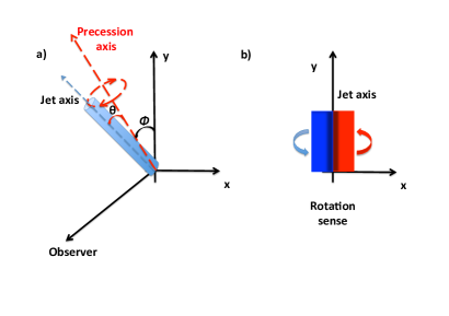
Figure 1.— Sketch of the simulation setup. In a) we show the general case in which we have a precessing jet observed at a given inclination angle $\phi$, which is the angle between the precessing axis with respect to the “plane of the sky” (the $x-y$ plane), whereas $\theta$ is the precessing angle of the jet axis measured from the precessing axis. The sense of the precession is also shown. In b) we show the sense of the jet rotation as seen by the observer for a rotating jet model in the plane of the sky.

As a final comment, the mean spectrum that has been subtracted from the datacube ($Q_{\lambda}$) can be reincorporated in the reconstructed datacube to recover the flux-calibrated data. The final product is a sequence of images (as a function of wavelength) in the real space:

$$(I^{\prime}_{ij\lambda}(\leq k_{\rm max}))_{0}=I^{\prime}_{ij\lambda}(\leq k_{\rm max})+Q_{\lambda}$$ (9)

from which one can reconstruct 2D images integrated in wavelength or select spectra from a given position in the images.

We will apply this formalism to our numerical simulations in the next section. We use PCA to mine data from numerical simulations as has been done for instance by Heyer & Schloerb (1997), Brunt, Heyer & Mac Low (2009) and Carrol, Frank & Blackman (2010). We will show that rotation and/or precession can appear in independent eigenvectors, and the PCA technique can therefore be used in the study of jet rotation to disentangle, in real data, signatures of rotation from other physical mechanisms, such as shocks and velocity asymmetries.

3. The numerical simulations

We apply the PCA analysis to the study of rotation in stellar jets by using synthetic emission maps generated by numerical simulations. The simulations presented here are the same shown previously in Cerqueira et al. (2006). The simulations were performed with the 3D hydrodynamic code YGUAZÚ-a (e.g. Raga et al., 2000). Briefly, we run 4 models of jets with pulsation period of $\tau_{p}=8$ years (see Table 1 and Figure 1). The M1 model, our reference jet model, is intermittent, with a jet velocity profile given by:

$$v_{j}=v_{0}\bigg{[}1+A{\rm sin}\bigg{(}\frac{2\pi}{\tau_{p}}t\bigg{)}\bigg{]}\,,$$ (10)

where $v_{0}=300$ km s^-1 and $A=0.33$. As discussed in Cerqueira et al. (2006), these values were chosen in order to reproduce the physical conditions of the DG Tau jet. Besides pulsation ( model M1), we include precession in M2 model, rotation in M3 model and precession and rotation in M4 model. For models with precession we adopt a period of precession equal to $\tau_{\theta}=8$ yr and an angle of precession $\theta=5^{\circ}$. The models with rotation have a rotational velocity profile given by:

$$v_{\phi}=8\;{\rm km}\;{\rm s}^{-1}\frac{R_{j}}{R}\,,$$ (11)

for $R>0.15R_{j}$, where $R_{j}$ is the jet radius (1$R_{j}=37.4$ AU) and $R$ is the cylindrical radius. In order to avoid a singularity at the jet axis, the rotational velocity is constant for $R\leq 0.15R_{j}$, and equal to $v_{\phi}=55$ km s^-1.

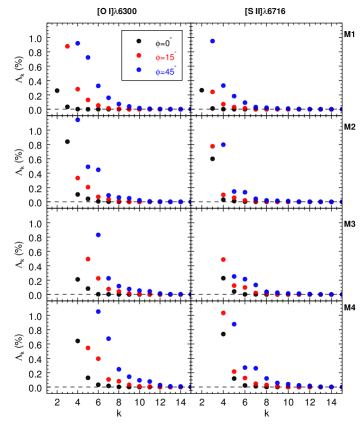
Figure 2.— Eigenvalues (in % of the variance) as a function of eigenvector’s order for models M1 to M4 (from top to bottom, respectively), for [O I]$\lambda$6300 (left) and [S II]$\lambda$6716 (right) emission lines. In each panel we show also the different inclinations considered: $\phi=0^{\circ}$ (black dots), $\phi=15^{\circ}$ (red dots) and $\phi=45^{\circ}$ (blue dots). The ordinate has been limited to 1.2% and the first eigenvalues are out of scale. However, they are given in Table 2, where we also provide all values until $k=10$. In each panel we have a horizontal, dashed black line, that was used to indicate the $k_{\rm max}$ for each curve (see the text for discussion).

The computational domain is a three-dimensional Cartesian box with spatial dimensions of $x=z=128$ and $y=512$ pixels. Each pixel has a physical dimension of 5.74 AU. We will present maps only for $i\leq 128$ and $j\leq 128$, since we are interested in the region near the jet inlet (the jet injection point at the computational domain).

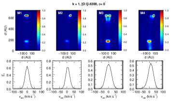
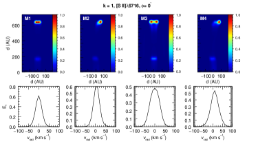
Figure 3.— First tomogram (${\bf T}_{i,j,k}$, for $k=1$) and eigenspectrum ($E_{k}$, for $k=1$) for models M1 to M4 (from left to right, respectively), for [O I]$\lambda$6300 (two topmost panel’s sequence) and [S II]$\lambda$6716 (two bottommost panels) emission lines at $\phi=0^{\circ}$. In each tomogram the distance from the jet inlet, in AU, is indicated. The color bar indicate the level of the (normalized) intensity. The eigenspectrum of each model is plotted below the respective tomogram.

Table 1 summarizes the main parameters of the models. To build the intensity matrix (equation 2) we construct velocity channel maps (VCM) around a given wavelength (see Cerqueira et al. 2006 for the details). For the forbidden emission lines [O I]$\lambda\lambda$6300,6363 and [S II]$\lambda\lambda$6716,6731 we calculate VCM from $v_{rad}=-400$ km s^-1 to +100 km s^-1, with a sampling of 10 km s^-1. Each channel map is one of the $m$ slices in $\lambda$ of the datacube, and we can build the intensity matrix $(I_{ij\lambda})_{0}$ for each $\lambda$ (or, alternatively, $m$ or $v_{rad}$).

In order to consider the effect of finite angular resolution we convolved each VCM with a Gaussian PSF with FWHM of $\sim 5$ pixels ($\sim$ 28.7 AU), or $0\farcs 21$ for a jet at a distance of Taurus (140 pc; see Kenyon, Dobrzycka & Hartmann, 1994), for example.

4. Eigenvalues, tomograms and eigenspectra

4.1. Eigenvalues and the scree test.

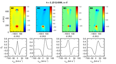
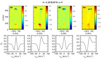
Figure 4.— The same as in Figure 3, but for $k=2$ (the second tomogram, ${\bf T}_{i,j,k}$, for $k=2$, and its respective eigenspectrum, $E_{k}$, for $k=2$).

In the PCA, it is important to know how many eigenvectors one must consider in the analysis. One way to determine this is to apply the scree test (Steiner et al., 2009), which is a visual test that is used to find the order $k$ where the eigenvalue levels off. To look at these $k$’s for our different models, emission lines and inclination angles with respect to the plane of the sky, we built diagrams of eigenvalues $\Lambda_{k}$ as a function of $k$. In Figure 2 we show the eigenvalues for models M1, M2, M3 and M4 (from top to bottom, respectively), for [O I]$\lambda$6300 (left) and [S II]$\lambda$6716 (right). The dots of different colors are associated with a specific inclination angle: black for $\phi=0^{\circ}$; red for $\phi=15^{\circ}$; blue for $\phi=45^{\circ}$. We note from Figure 2 that the eigenvalues go to $\sim 0$ after a given $k=k_{\rm max}$. In order to help to find these $k_{\rm max}$, we have drawn a horizontal line in each plot at a constant $\Lambda_{{\rm threshold}}=10^{-3}$ %. The first point (for each model, inclination and emission line) intercepted by this horizontal line defines the $k_{\rm max}$. In Appendix A we present in Table 2 the first ten eigenvalues for each one of the models. We present also the number of relevant eigenvectors as determined by the criteria of the scree test (see Table 3). This means that for each combination of parameters (model, emission line and inclination angle) we have an already predefined number of eigenvectors that we must look in searching for relevant uncorrelated phenomena. However, we used higher order eigenvectors to perform a complete analysis of the problem, although they will not be presented here due to the lack of space.

4.2. Tomograms and eigenspectra

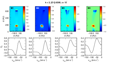
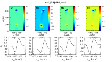
Figure 5.— Second tomogram (${\bf T}_{i,j,k}$, for $k=2$) and eigenspectrum ($E_{k}$, for $k=2$) for models M1 to M4 (from left to right, respectively), for [O I]$\lambda$6300 (two topmost panel’s sequence) and [S II]$\lambda$6716 (two bottommost panels) emission lines at $\phi=15^{\circ}$. In each tomogram the distance from the jet inlet, in AU, is indicated. The color bar indicate the level of the (normalized) intensity. The eigenspectrum of each model is plotted below the respective tomogram.

To obtain an image in the new coordinate system, or tomogram (or also an eigenimage; see Heyer & Schloerb 1997), we use equations (3) and (5). A column in the data matrix (see equation 5) can be then transformed in a image, that is the projection of the datacube (in the new coordinate system) onto the chosen eigenvector (of order $k$). The eigenvector, on the other hand, is a linear combination of the original (spectral) coordinates, and its coefficients, or weights, can be both positive or negative. Viewed as a plot of weight versus radial velocity, the eigenvector is called eigenspectrum. Therefore, a tomogram can displays either positive or negative regions, that are related with the weights in the corresponding eigenspectrum. This will allow us to investigate both and identify some kinematical “properties”, like jet precession or rotation.

4.2.1 Jet or precessing axes in the plane of the sky ($\phi=0^{\circ}$)

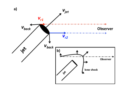
Figure 6.— a) Geometry for a jet inclined towards the observer. Lateral backflowing material with velocities $v_{back}$ compose with the jet velocity and favors high radial velocities in the half bottom of the jet cross section (as seen by the observer; indicated by the blue arrow and with velocity $v_{r2}$) in comparison with the half top part of the jet cross section (red arrow with velocity $v_{r1}$). Both are blueshifted velocities but appear in the tomogram of the model M1 in of Figure 5 as a red and blue regions. b) An inclined bow shock can also explain the tomograms/eigenspectra of the model M1 and cannot be ruled out in the case of the internal working surface, where the internal bow shock propagates faster than the leading one due to the non-stationarity of the ambient medium ahead of it.

In Figure 3 we show the first tomogram ($k=1$) and its associated eigenspectrum for models M1 to M4 (from left to right), for [O I]$\lambda$6300 (top) and [S II]$\lambda$6716 (bottom) emission lines, at $\phi=0^{\circ}$. The color bar in the tomograms (from here and after) represent a non-dimensional quantity, since pixel’s intensities have been normalized to the maximum value in each tomogram. Distances, in AU, are indicated in the ordinate of the leftmost tomogram, as well as in each abscissa. For the eigenspectra, the weights are plotted as a function of the radial velocity in km s^-1. These $k=1$ eigenvectors for each model (see Table 2) present tomograms that are similar to an integrated image in the respective emission line. They emphasize the presence of the two working surfaces: one internal near to the jet inlet, and the leading one at the tip of the jet, where most of the emission comes from the radiative losses behind the shocks. This eigenvector traces the most important shocks in the system. The respective eigenspectra peak at $\sim$ 0 km s^-1 in the case of models M1 and M3, and at $\sim$ 10 km s^-1 in the precessing cases M2 and M4 (M4 also has rotation besides precession).

In Figure 4 we show the second tomogram ($k=2$) and its associated eigenspectrum for models M1 to M4 (from left to right), for [O I]$\lambda$6300 (top) and [S II]$\lambda$6716 (bottom) emission lines, at $\phi=0^{\circ}$.

For M1 model (panels in the first column), this eigenvector contributes to 0.2597% and 0.2655% of the variance (for [O I] and [S II], respectively; see Table 2) and traces velocity gradients at the jet head (for both emission lines; their tomograms and eigenspectra are equivalent) that are perpendicular to the jet axis, but symmetric with respect to it.

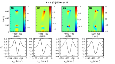
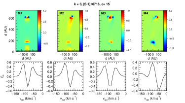
Figure 7.— The same as in Figure 5, but for $k=3$ (the third tomogram, ${\bf T}_{i,j,k}$, for $k=3$, and its respective eigenspectrum, $E_{k}$, for $k=3$).

The tomograms for the M2 (precessing) model (panels in the second column of the Figure 4) are considerably different for the two emission lines. In the case of the [O I]$\lambda$6300, the tomogram combined with its eigenspectrum clearly traces the precession of the jet axis. The eigenspectrum has anti correlated wings: the red wing of the line, associated with positive weights and positive regions in the tomogram, traces the receding portion of the jet (coincident with the internal working surface near to the jet inlet), while the blue wing of the line, associated with negative weights and negative regions in the tomogram, traces the approaching jet. We note that there is also a positive gradient, from the internal working surface (hereafter, IWS) up to the jet head, in the tomogram’s intensity along the jet. The eigenspectrum for the [S II]$\lambda$6716 emission line also depicts the same anti correlation in the wings of the line, but here the interpretation is not as straightforward as before. In the eigenspectrum, there is only one peak for each positive and negative weights. This suggests that all blue regions in the tomograms are blueshifted with respect to the red ones. According to this interpretation, the IWS is receding and there is a smooth gradient in blue regions from the IWS towards the jet head suggesting the precession. However, at the jet head seen in the tomogram we have a strong gradient in radial velocity, and the anti correlation seen in the eigenspectra in this case may be due to a combination of these two features, and could not be attributed only to the precession. We note that a signature for the precession can be found in all tomograms until $k=4$ (not shown here).

The second eigenvector for M3 (rotating) model accounts for 6.7645% and 3.9785% of the variance in the dataset for [O I]$\lambda$6300 and [S II]$\lambda$6716 emission lines, respectively (Table 2). Their tomogram/eigenspectrum are in the third column of the Figure 4. The eigenspectrum for the [O I]$\lambda$6300 emission line indicates again an anti correlation between both wings of the line. Negative weights are associated with negative regions (blue regions) in the tomogram, indicating a receding jet (it is in the red wing of the line), while positive weights, in the blue wing of the line, indicate that the red regions in the tomogram are approaching. This is consistent with the sense of the rotation imposed at the beginning of our simulation. This eigenvector for [O I] traces, then, the rotation of the jet. Conversely, the same tomogram and the eigenspectrum for the [S II]$\lambda$6716 emission line are completely symmetric with respect to the jet axis and to the zero radial velocity, respectively. There is no trace at all for the presence of the rotation in this tomogram for this emission line. It will appear only in the third eigenvector (not show here).

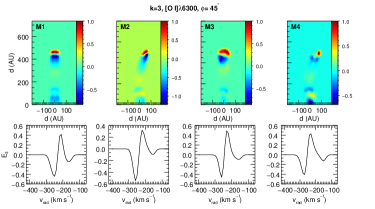
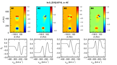
Figure 8.— Third tomogram (${\bf T}_{i,j,k}$, for $k=3$) and eigenspectrum ($E_{k}$, for $k=3$) for models M1 to M4 (from left to right, respectively), for [O I]$\lambda$6300 (two topmost panel’s sequence) and [S II]$\lambda$6716 (two bottommost panels) emission lines at $\phi=45^{\circ}$. In each tomogram the distance from the jet inlet, in AU, is indicated. The color bar indicate the level of the (normalized) intensity. The eigenspectrum of each model is plotted below the respective tomogram.

The second eigenvector for M4 (rotating and precessing) model accounts for 18.007% and 12.7514% of the variance of the data, for the [O I]$\lambda$6300 and [S II]$\lambda$6716 emission lines, respectively. Their tomogram/eigenspectrum are in the fourth column of the Figure 4. The tomogram and the eigenspectrum for the [O I]$\lambda$6300 emission line shows anti correlation between both sides of the jet axis near to the jet inlet only. Positive regions, red in the tomogram, are correlated with the positive, red wing of the line, while negative regions, blue in the tomogram, are correlated with negative weights in the blue wing of the line. This is consistent with the interpretation that the jet is rotating, and the correct jet rotation sense is recovered. From the IWS until the jet head the jet is dominated by blue, negative regions. The gradient seen in the tomogram can suggest a precession. For the [S II]$\lambda$6716 emission line the situation is less clear. Some asymmetries with respect to the jet axis can be detected near to the jet inlet, but it is not obvious that rotation is involved. The eigenspectrum seems to reflects the gradient in radial velocity at the jet head, which is in turn very similar to the one detected in the M2 model for this same tomogram.

In the following sections, we will not show the first tomograms anymore (i.e., tomograms for $k=1$): they are always similar to an image in the real space of the integrated emission line and they do not contribute to our present purposes, which is the search for evidence of rotation and precession in jets.

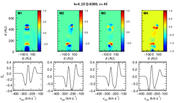
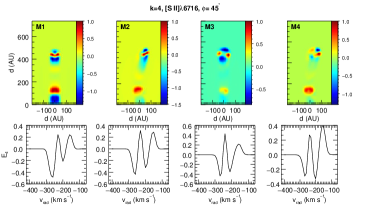
Figure 9.— The same as in Figure 8, but for $k=4$ (the fourth tomogram, ${\bf T}_{i,j,k}$, for $k=4$, and its respective eigenspectrum, $E_{k}$, for $k=4$).

4.2.2 Tomograms for moderately inclined systems ($\phi=15^{\circ}$)

In Figure 5 we show the second tomogram ($k=2$) and its associated eigenspectrum for models M1 to M4 (from left to right), for [O I]$\lambda$6300 (top) and [S II]$\lambda$6716 (bottom) emission lines, at $\phi=15^{\circ}$. All eigenspectra are blueshifted in comparison with the models in previous section, as expected for jets that are pointing towards the observer. They also present anti correlation between the red and blue wings of the line, no matter if we are looking for a simple, non-precessing and non-rotating (M1) model or a complex (M4) one, and this fact deserves a careful analysis.

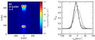
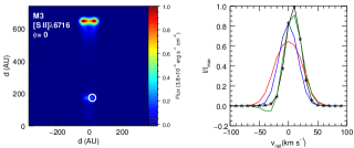
Figure 10.— Images (left) of the collapsed original datacube for the M3 (rotating) model around the [O I]$\lambda$6300 (top) and [S II]$\lambda$6716 emission lines. Spectra (right) have been extracted from the area indicated by the white circles in the images using the original datacube (black solid line), and the reconstructed datacubes considering eigenvectors until $k_{\rm max}=1$ (red), $k_{\rm max}=2$ (blue), $k_{\rm max}=3$ (green) and $k_{\rm max}=4$ (black stars). Fluxes are normalized to unity, and each maximum is indicated in the right side of the color bars. In the extracted spectra, intensities are also normalized with respect to the maximum of the integrated spectra (black solid line). The circles in the images have a diameter of 4 pixels, or 22.9 AU. This corresponds to $0\farcs 16$ considering the distance to Taurus (140 pc), for example. The origin of the coordinate system corresponds to the position of the jet inlet, and distances from the origin are indicated in AU.

In the case of the reference model M1, the structures (positive/negative regions) in the tomogram are symmetric with respect to the jet axis. The portions of the jet immediately behind the working surfaces (at $d(y)\leq 150$ AU and at 550 AU $\leq d(y)\leq$ 600 AU) are correlated with the negative weights of the eigenspectra for both emission lines (see the first column of Figure 5), and then, they are correlated with the blue wing of the emission line. Beyond these limits (that is, for $d(y)\sim 180$ AU and $d(y)\sim 630$ AU), the tomograms display positives (see the color bar in each figure) regions, that are correlated with the red wing of the line. We interpret these structures at the jet working surfaces as a signature of the backflowing post-shocked material, that escapes laterally at the Mack disk (or jet shock), favoring lower (absolute) radial velocities on the top half of the jet cross section, and, analogously, higher (absolute) radial velocities on the bottom half of the jet cross section. In Figure 6 (a) we present a cartoon summarizing the interpretation. We note that an inclined bow shock could also account for the blue/red asymmetry in the line and cannot be ruled out (see the sketch presented also in Figure 6-b), particularly for the case of an IWS, for which the bow shock propagates into a non-stationary ambient medium. In this case this effect can be more noticed since we expect high bow shock velocities in comparison with the leading bow shock.

The precessing model M2 also show an asymmetric eigenspectrum. In the [O I]$\lambda$6300 emission line, the tomogram essentially traces the IWS near the jet inlet. It is a positive region (red in the color bar), correlated with the positive weights that are present in the red wing of the line, as we can see in the eigenspectrum. There is a clear contrast between positive (internal emission knot) and negative regions (the jet head), suggesting a precession. However, positive weights dominate the eigenspectrum (it has a maximum that is more than three times the negative peak at $v_{rad}=-90$ km s^-1), which is evident also in the tomogram. For the [S II]$\lambda$6716 emission line, the contrast between positive and negative weights is less intense and the structures more clear. There is a gradient in the negative region that goes from the IWS and peaks at the jet head. There, we have also a positive region, suggesting that the same effect explored in Figure 6 may also be present. However, the precession breaks the symmetry with respect to the jet axis.

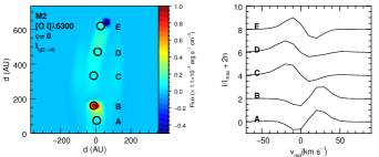
Figure 11.— Images (left) and spectra (right) from the reconstructed datacube for the precessing model M2 at $\phi=0^{\circ}$, for the [O I]$\lambda$6300 (top) and [S II]$\lambda 6716$ (bottom) emission lines. Eigenvectors from 2 to 4 were used in the reconstruction process, since they have signatures for the jet precession. Circles labeled from A to E mark the positions where a spectrum has been extracted. They are in the right side panels, normalized to unit. We added a constant 2$n$, where $n=0-4$ to the spectra at positions A to E, respectively, in order to separate them in different levels, to improve the visualization. The images are integrated in wavelength.

For the M3 (rotating) model (third column in Figure 5), the second tomogram shows positive (red) and negative (blue) regions that are distorted with respect to the jet axis. The region that extends from the jet inlet until the IWS is blue in the left side of the jet axis for both emission lines (although more clearly seen in the tomogram associated with the [O I]$\lambda$6300 emission line). At the tip of the IWS, the red (positive) region is distorted toward the right side of the jet axis, indicating that this side of the jet is more redshifted than the other one (since positive weights in the eigenspectra are in the red wing of the line; see the eigenspectrum associated with this model in the third column of Figure 5). At the jet head, the rotation signature is evident only in the case of the [S II]$\lambda$6716 emission line: we can interpret the blue/red region in the jet head in this tomogram as in the case of model M1, and attributes to the rotation the cause for the observed asymmetry with respect to the jet axis.

The second eigenvector for the model M4 contributes to 33.2961% and 14.5136% of the variance in the dataset for [O I]$\lambda$6300 and [S II]$\lambda$6716 emission lines, respectively, at $\phi=15^{\circ}$. The tomogram and eigenspectrum can be seen in the last column of the Figure 5. Again, the eigenspectra for both emission lines show blue/red wing asymmetry. The tomograms are, however, different. For the [O I]$\lambda$6300 emission line, positive regions in the tomogram are concentrated in the IWS. It has a peak on the right side of the jet axis, showing an asymmetric distribution in intensity with respect to the jet axis (as in the case of the M3 model). All other parts of the jet are mostly dominated by blue, negative regions, with a maximum at the jet head. There is a negative gradient from the jet inlet to the IWS, and then a positive gradient from the IWS up to the jet head, which is suggest the precession. Although the eigenspectra are similar for the [S II]$\lambda$6716 emission line in comparison with the one for the [O I]$\lambda$6300 emission line, their tomograms are not. Both positive and negative regions peaks at the jet head, suggesting that the anti correlation in the wings of the line are related to gradients in velocity at the jet region.

In Figure 7 we show the tomograms (first and third rows of panels) and eigenspectra (second and fourth rows of panels) for models M1 to M4 (from left to right) at $\phi=15^{\circ}$ and $k=3$. As before, the two topmost panels refer to the [O I]$\lambda$6300 emission line, while the two bottommost panels concern the [S II]$\lambda$6716 emission line. There is a pattern in the eigenspectra that is almost the same for all cases: there is an interval in radial velocity of negative weights, bracketed by two peaks of positive weights, which make the interpretation far less obvious. In particular, a negative region in a given tomogram can be either red- or blue-shifted with respect to a positive one. The same “color” in a tomogram can, in this case, be indicative of different kinematics, and the interpretation is actually difficult.

M1 model (leftmost column in Figure 7) has tomograms that show negative/positive regions that peak at the jet head (for both emission lines). The positive (red) regions at the jet head are correlated now with positive weights in the eigenspectra, since the maximum in both tomograms is localized in this region. Then, the negative region just above it in the case of [O I]$\lambda$6300 emission line, and the negative regions symmetrically displaced with respect to the jet axis in the case of [S II]$\lambda$6716 emission line are redshifted in comparison with the red regions at the jet head, as we can see in the eigenspectrum. This interpretation is still compatible with the scenario proposed in Figure 6. The same is true for the IWS, which correlates with the positive/negative peaks at $v_{rad}=-50$ and -80 km s^-1, respectively. The yellow (positive) region in the jet base can be only correlated with the positive weights at the bluemost wing of the line in the eigenspectra.

M2 model (panels in the second column of Figure 7) shows that the highest values for the positive and negative regions in the tomogram occur at the jet head. Negative regions are concentrated at the jet tip, while the positive regions are immediately behind of it, with a negative gradient of intensities from the jet head until the IWS. The peak in the positive weights of both eigenspectra (i.e., for both emission lines) is at $v_{rad}=-100$ km s^-1, that are in the blue wing of the lines. This means that the negative blue region on top of these positive regions at the jet head are redshifted with respect to them, since the negative weights in the eigenspectra are at lower (absolute) radial velocities ($\sim-60$ km s^-1).

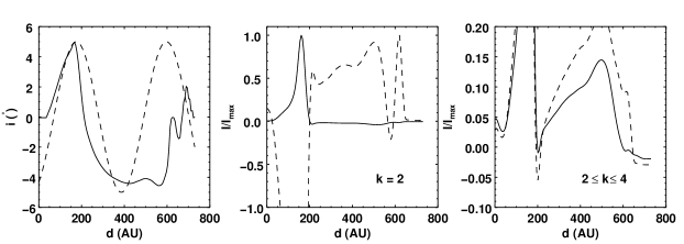
Figure 12.— Left:) The inclination of the jet axis with respect to the plane of the sky, here defined as $i$, as a function of the vertical distance from the jet inlet for the model M2 (precessing jet), estimated from the simulation (solid line), using velocities taken in a straight line along the $y-$coordinate, starting at the jet inlet at $x=y=0$. The dashed line is an arbitrary cosine function. Middle:) Normalized fluxes taken from the reconstructed datacube considering only the second eigenvector ($k=2$) (solid line: [O I]$\lambda$6300; dashed line: [S II]$\lambda$6716). Right:) The same as in the middle panel but using the eigenvectors $2\leq k\leq 4$ to reconstruct the datacube. The fluxes have been normalized to their maximum value in each curve. In the rightmost panel, we have limited the ordinate to 0.2.

The third tomogram for the M3 and M4 models (third and fourth columns of panels in Figure 7, respectively) at $\phi=15^{\circ}$ show a twisted pattern in the regions of positive and negative values, which is more evident for the [O I]$\lambda$6300 emission line in comparison with the [S II]$\lambda$6716 emission line. We can interpret this behavior saying that negative regions in the tomograms can be both redshifted or blueshifted with respect to positive regions placed in a symmetric position with respect to the jet axis. This is because the negative peaks in the eigenspectra for both models are bracketed by two positive peaks, and that it is an effect of the rotation, that changes the tomograms with respect to the non-rotating M1 and M2 models even if the eigenspectra have the same shape/form. However, by analyzing only this eigenvector, the presence of such a twisted feature in the tomograms does not allow us to say/conclude anything about the rotation sense of the jet.

Unlike the case of $\phi=0^{\circ}$ shown in the previous section, evidences for the rotation here are more subtle. The mere fact that we are “observing” the jet at a non-null inclination angle makes the analysis of the principal components more difficult.

4.2.3 Tomograms for highly inclined systems ($\phi=45^{\circ}$)

At $\phi=45^{\circ}$, the dataset becomes even less redundant with an appreciable amount of variance distributed in higher order eigenvectors. In Figures 8 and 9 we show as an example the third and fourth tomograms/eigenspectra, respectively, for models M1 to M4 at $\phi=45^{\circ}$. As before, the results for the [O I]$\lambda$6300 (topmost two panels) and [S II]$\lambda$6716 (bottommost two panels) emission lines are shown. Some of the patterns already discussed can be seen here too. Eigenspectra becomes more complex, in part due to gradients in velocity at the jet head. The clumpy, alternating pattern observed there specially in models M3 and M4 (for $k=3$ and $k=4$) makes the kinematic analysis, and its interpretation, more difficult. The presence of the rotation, for instance, is only suggested near the jet inlet in the $k=4$ tomograms of model M3 (and it is not so evident for the M4 model; see Figure 9). It is present also in higher order tomograms (not shown here).

We conclude that it is not possible to express, or to describe, the precession and/or the rotation with a single eigenvector, unless if the precession/jet axis lies in the plane of the sky. We have actually a collection of eigenvectors for which the signature for the precession and/or for the rotation can be found. In general, the higher the inclination angle $\phi$, the higher will be the eigenvector’s order in which they will manifest. In this Section we have discussed the most relevant eigenvectors. Furthermore, the interpretation of higher order tomograms becomes less and less evident, with eigenspectra showing several negative and positive successive peaks.

5. PCA signatures for precession and rotation from reconstructed datacubes

In this section we will present images from reconstructed datacubes, obtained using the equation (8) for a collection of eigenvectors that are representative of a given feature (see Appendix B). We will also discuss the properties of spectra extracted at fixed spatial positions obtained from reconstructed datacubes. We note that all images presented in this section are actually integrated in wavelength.

Before entering into the details of our results, and as a test for the method, we can choose a region in a given image and reconstruct, step by step, the line profile using a certain number of eigenvectors. In Figure 10 we show the integrated (non treated by the PCA) images of the [O I]$\lambda$6300 (top panel) and [S II]$\lambda$6716 emission lines (bottom panel) for the M3 (rotating) model. Superimposed on the images we show circles (of 22.9 AU of diameters; which corresponds to $0\farcs 16$ at 140 pc of distance) to indicate the position where spectra have been extracted. The spectra are on the right panels (black, solid lines). We also show line profiles obtained from the reconstructed datacube, keeping in the reconstruction procedure an increasing number of eigenvectors from 1 to 4 (see equation 8): $k_{\rm max}=1$ (red curve), $k_{\rm max}=2$ (blue curve), $k_{\rm max}=3$ (green curve) and $k_{\rm max}=4$ (black stars). In this example, the reconstructed profiles converge very well to the original one for both emission lines (the properties and features of the profiles will be discussed in the next Section), using only 4 eigenvectors.

5.1. Jets in the plane of the sky

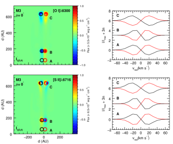
Figure 13.— Reconstructed images (left) and extracted spectra (right) for Model M3 at $\phi=0^{\circ}$ and for [O I]$\lambda$6300 (top) and [S II]$\lambda$6716 (bottom) emission lines. Different eigenvectors have been considered to reconstruct the datacube: $k=2$ and 4 for [O I]$\lambda$6300 and $k=3$ and 4 for [S II]$\lambda$6716 lines, as indicated in the bottom left part of each image. Spectra were extracted at symmetrical positions, labeled A, B and C, with respect to the jet axis. The colors of the solid lines (right panels) corresponds to the color of the slits. Distances from the jet inlet are indicated in AU in images. Spectra are normalized and we have added to their intensity a constant 3$n$, with $n=$ 0, 1 and 2 at the positions A, B and C, respectively. The images are integrated in wavelength.

In Figure 11 we show the image (left panels) and spectra (right panels) obtained from the reconstructed datacube for the model M2 (precessing model) at $\phi=0^{\circ}$ (which means that the axis of precession is coincident with the $y-$axis). As discussed in Section 4 (Section 4.2.1), we have identified the precession in eigenvectors’ orders $2\leq k\leq 4$ among the eigenvectors suggested by the scree test (see Table 3). The datacube was then reconstructed considering these three eigenvectors. For the sake of clarity and to allow the comparison between them, the results for the [O I]$\lambda$6300 and [S II]$\lambda$6716 emission lines are shown. The emission line is indicated in the top-left corner of each image. We choose different positions along the jet to extract a spectrum. These regions are indicated by circles superimposed in the image (as in Figure 10, the size of the circle is representative of the collected area which means $0\farcs 16$ at a distance of 140 pc, for example). Viewing from the base of the jet (region A) up to its tip (region E), each spectrum peaks at different radial velocities, suggesting clearly a precession pattern. Assuming as an upper limit for the jet velocity $v_{j,lim}<400$ km s^-1 (see equation 10), we can estimate the radial velocity to be of the order of $|v_{rad}|\leq v_{j,lim}{\rm sin}\theta$, or $|v_{rad}|\leq 34$ km s^-1. The emission peaks fall well within this limit.

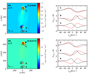
Figure 14.— Reconstructed images (left) and extracted spectra (right) for Model M4 at $\phi=0^{\circ}$ and for [O I]$\lambda$6300 (top) and [S II]$\lambda$6716 (bottom) emission lines. Different eigenvectors have been considered to reconstruct the datacube: $k=2$ to 8 for the oxygen and $k=2$ to 7 for the sulfur lines, as indicated in the bottom left part of each image. Spectra were extracted at symmetrical positions, labeled A, B and C, with respect to the jet axis. The colors of the solid lines (right panels) corresponds to the color of the slits. Distances from the jet inlet are indicated in AU. Spectra are normalized and we have added to their intensity a constant 3$n$, with $n=$ 0, 1 and 2 for spectra at the positions A, B and C, respectively. The images are integrated in wavelength.

Figure 11 indicates that there is a variation in the flux along the jet length that can be due to changes of the viewing angle. In Figure 12 we try to correlate these quantities. For a fixed $x-$coordinate at the jet inlet ($x=0$), we compute ${\rm tan}^{-1}(v_{rad}/v_{y})$ along the jet length, which is an estimate for the angle $i$ that the jet axis makes with the precession axis that lies in the plane of the sky (the $y$ axis at $x=0$). In this equation, $v_{rad}$ and $v_{y}$ are the velocities parallel and perpendicular to the line of sight, respectively, taken from the simulation. This quantity is plotted in the leftmost panel in Figure 12 (solid line), where we show also an arbitrary cosine function (dashed line). In the middle and right panels we show the flux in the [O I]$\lambda$6300 (solid line) and [S II]$\lambda$6716 (dashed line) emission lines, taken along the precession axis from the reconstructed datacube, considering the eigenvectors with $k=2$ (middle panel) and $2\leq k\leq 4$, respectively. The abrupt variation of the intensity along the jet seems to correlates with the variation in the inclination angle when we consider the combined eigenvectors (rightmost panel).

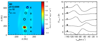
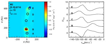
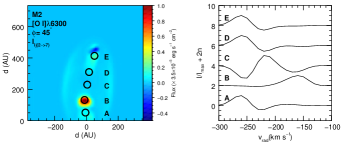
Figure 15.— Reconstructed images (left) and spectra (right) for the precessing model M2 for $\phi=15^{\circ}$ (first and second panels, from top to bottom) and $\phi=45^{\circ}$ (last two bottom panels), for [O I]$\lambda$6300 (first and third rows) and [S II]$\lambda$6716 (second and fourth rows) emission lines. Different eigenvectors have been used in the reconstruction procedure. Their range is show at the top left of each image. Circles labeled from A to E mark the positions where a spectrum has been extracted. They are in the right side panel, normalized to unit (we added a constant 2$n$, $n=0-4$ from A to E, in each spectra in order to separate them in different levels). The images are integrated in wavelength.

In Figure 13 we show images (left) and spectra (right) from the reconstructed datacube for the [O I]$\lambda$6300 (top) and [S II]$\lambda$6716 (bottom) emission lines, for the rotating M3 model observed at $\phi=0^{\circ}$. For the [O I]$\lambda$6300 line, we have found evidence for rotation in the eigenvectors 2, 4, 7, 9, 12 and 14 (this is not a comprehensive list). For the [S II]$\lambda$6716 line, the eigenvectors associated with the rotation are 3, 4, 7, 9, 12 and 14. The scree test (see Section 4) suggests for this model, however, that the relevant eigenvectors are those with $k\leq 6$ (see Table 3 and Figure 2). We have, then, restricted the relevance of the eigenvectors in the reconstruction procedure up to this limit. In these two images we placed artificial slits at increasing distances from the jet inlet, at positions labeled A, B and C. The slits are symmetrically displaced in pairs with respect to the jet axis. The extracted spectra are plotted in the right panels (the colors of solid lines used to draw each spectra are associated with the color of the “apertures” in the FoV). The peaks of red/black curves suggest that the jet material at the right side of the jet axis is receding, while the left side is approaching, recovering the sense of the jet rotation imposed initially, independent of the position along the jet axis A, B or C.

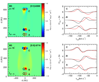
Figure 16.— Reconstructed images (left) and extracted spectra (right) for Model M3 at $\phi=15^{\circ}$ and for [O I]$\lambda$6300 (top) and [S II]$\lambda$6716 (bottom) emission lines. To reconstruct the datacube we have used the eigenvectors $k=2$, 3, 4 and 6 for oxygen and $k=2$ to 5 for the sulfur emission lines, as indicated in the bottom left part of each image. Spectra were extracted at symmetrical positions with respect to the jet axis, labeled A, B and C. The colors of the solid lines (right panels) corresponds to the color of the slits. Distances from the jet inlet are indicated in AU. Spectra are normalized and we have added to their intensity a constant 3$n$, with $n=$ 0, 1 and 2 at the positions A, B and C, respectively. The images are integrated in wavelength.

In Figure 14 we show images (left) and spectra (right) from the reconstructed datacube for the (rotating/precessing) model M4, in the [O I]$\lambda$6300 (top) and [S II]$\lambda$6716 emission lines. For this case, we have evidence for rotation and precession in several eigenvectors with order higher than 2. We then keep the eigenvectors from 2 to 8 and from 2 to 7 in the reconstruction process of the datacube for oxygen and sulfur emission lines, respectively, obeying the limits suggested by the scree test (see Table 3). We have extracted spectra in pairs that do not follow a straight line along the $y-$axis but instead, we place the slits along a “suggested” jet symmetry axis (see Figure 14). We see in the spectra that there is evidence for the precession: radial velocities peaks for slit pairs changes from positive to negative values from B to C, indicating that jet material in B is receding while in C it is approaching, as expected. There is also an indication for rotation, since the red curves peaks are always redshifted with respect to the black curve, as we should expect considering the sense of the jet rotation.

5.2. Inclined systems

In Figure 15 we show the images (left) and spectra (right) for the (precessing) model M2 at $\phi=15^{\circ}$ (two upper panels) and at $\phi=45^{\circ}$ (two bottom panels), for different emission lines, as indicated in each figure. Each image/spectrum has been obtained from a reconstructed datacube, using those eigenvectors that indicate the presence of the precession in each case: $k=2$, 3, 4 and 6 for the $\phi=15^{\circ}$ (first and second rows); $2\leq k\leq 7$ for the oxygen line at $\phi=45^{\circ}$ (third row of panels) and $2\leq k\leq 5$ for sulfur line at $\phi=45^{\circ}$ (bottom panel). We can see that the peaks of the emission lines indicate the presence of precession, and that it is consistent with the pattern of the precession obtained for model M2 (for $\phi=0^{\circ}$; left panel in Figure 12). As we increase the inclination angle, the amplitude of the variation of the radial velocity increases (bottom panels). The scenario is independent of the emission line, although maps from [O I] and [S II] may differ considerably.

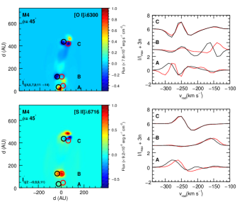
Figure 17.— Images (left) and spectra (right) for model M4 at $\phi=45^{\circ}$, for [O I]$\lambda$6300 (top) and [S II]$\lambda$6716 (bottom) emission lines. In the reconstruction process of the datacube we have used eigenvectors $k=4$, 5, 7, 8, 11, 12, 13 and 14 for the oxygen emission line and $k=2$ to 6, and $k=8$, 9 and 11 for the sulfur emission line, as indicated in the bottom left part of each image. Spectra were extracted in pairs, along and across the jet length, at different positions labeled A, B and C. The colors of the solid lines (right panels) corresponds to the color of the slits. Distances from the jet inlet are indicated in AU in images. Spectra are normalized and we have added to their intensity a constant 3$n$, with $n=$ 0, 1 and 2 at the positions A, B and C, respectively. The images are integrated in wavelength.

Eigenvectors 2, 3, 4 and 6 have been used to reconstruct the datacube for the (rotating) M3 model, at $\phi=15^{\circ}$ for the [O I]$\lambda$6300 emission line, while eigenvectors from 2 to 5 were used to reconstruct the datacube around the sulfur line for the same model and inclination angle. In Figure 16 we show, as in the previous figures, the reconstructed image and several spectra, extracted along and across the jet axis. As in the case of $\phi=0^{\circ}$ (see Figure 13), spectra from red slits (right side of the jet axis) are always redshifted in comparison with spectra from black slits (positioned on the left side of the jet axis), suggesting that the jet is rotating and recovering the initial rotating sense. These peaks occur, however, at different radial velocities. While in A and C the spectra peaks at $v_{rad}\sim-100$ km s^-1, in B they peaks at $v_{rad}\sim-60$ km s^-1. This difference may be due to the presence of an internal working surface in B. Another potential source for this difference is the fact that jet velocity is time variable (see equation 10), and this lower (absolute) value for the radial velocity is consistent with the one expected when the jet velocity is in its minimum, $v_{j,min}=200$ km s^-1, when projected at $\phi=15^{\circ}$.

In the more complex case in which we have rotation and precession, as in model M4, we can see the same effect (in all the emission lines). In Figure 17 we show images (left) and spectra (right) for the model M4, for [O I]$\lambda$6300 (top) and [S II]$\lambda$6716 emission lines. The eigenvectors used in the reconstruction process are indicated in the bottom-left corner of each figure. The pattern observed in the spectra is consistent with a rotating and velocity variable jet. However, the spectra are substantially more fuzzy in comparison with those obtained for this same model and emission lines at small inclination angles (see Figure 14).

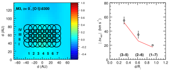
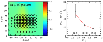
Figure 18.— Array of slits superimposed on the reconstructed image, zoomed at the jet inlet (left panels). The array of 4$\times$7 slits disposed across and along the jet length is equivalent to that of Cerqueira et al. (2006). The open circles in the right panels are the mean values of the radial velocity shift from symmetrically disposed slits (3-5), (2-6) and (1-7), considering the four different regions (from I to IV). The error bars indicate the dispersion around the mean value. The red solid line is obtained calculating analytically $\Delta v_{rad}=2\times v_{rad}$, where $v_{rad}=8{\rm cos}\phi\cdot R_{j}/R$. In the top panels we have the result for M3 model at $\phi=0^{\circ}$ and in the bottom panel, $\phi=15^{\circ}$. In all cases, the emission line is the [O I]$\lambda$6300. The images are integrated in wavelength.

In Figure 18 we attempt to recover the initially imposed rotational profile using the reconstructed datacube. We build an array of 4$\times$7 slits, or four regions (I to IV) at increasing distances from the jet inlet and seven positions (1 to 7) across the jet axis. The size of the slits and their distribution follow those of Cerqueira et al. (2006). For each extracted profile we take the radial velocity of the peak, and calculate the difference (i.e., the radial velocity shift) for each pair of slits displaced symmetrically with respect to the jet axis: (3-5), (2-6) and (1-7). Each region (from I to IV; see Figure 18) contributes to one radial velocity shift for each slit pair, and the mean value for a such radial velocity shift is plotted as a function of the distance from the jet axis in the right panel of the Figure (open circles; the error bar gives the dispersion around the obtained mean value). In order to compare with the initially imposed rotational profile, we calculate for each radial distance the expected (at $t=0$) radial velocity shift (for $R>0.2R_{j}$): $|\Delta v_{rad}|=2\times 8\cdot{\rm cos}\phi(R_{j}/R)$, where the ${\rm cos}\phi$ accounts for the inclination (red, solid curve in Figure 18). Although the match is reasonable for both inclinations ($\phi=0^{\circ}$ and $\phi=15^{\circ}$), we can not reproduce the original profile for the case of $\phi=45^{\circ}$. The method applied here fails also to recover the original profile in the case where rotating and precession are combined, as in model M4.

6. Conclusions

The PCA technique has been extensively applied in the astrophysical context (e.g., Steiner et al., 2009; Ricci et al., 2011; Malyshev, 2012). PCA is used to identify quickly in large datasets patterns and correlations that otherwise would not be revealed. These patterns can then be interpreted in terms of arising from physically uncorrelated phenomena present in the system, that thanks to PCA can be separated, identified and studied in detail. PCA offers also an efficient way to remove unwanted features from the data, as noise or instrumental fingerprints, and to compress and transmit only the relevant information present in a large dataset. We describe briefly the method in Section 2. The PCA method can be fruitfully applied to the analysis of spectro-imaging data like those provided by observations of diffuse targets with Integral Field Spectroscopy as shown in Steiner et al. (2009); Ricci et al. (2011), who apply PCA to observations of galaxies. In general, the interpretation of the observational data based on PCA tomograms is highly improved with the help of three-dimensional numerical experiments. This has been shown, for example, in Heyer & Schloerb (1997), Brunt, Heyer & Mac Low (2009) and Carrol, Frank & Blackman (2010). In this paper we show the potential applicability of the PCA to the study of HH jets by using the results of three-dimensional numerical simulations of rotating, precessing jets.

We apply the PCA to the synthetic images produced from the simulations, where we control the presence of known physical phenomena. We use the PCA to test if signatures of these phenomena can be isolated in the data, and produce a benchmark of PCA tomograms, with which PCA-processed real IFU observations of jets can be compared. In this work, we started generating from the simulations spectro-imaging datacubes around the wavelength of relevant emission lines for four different jet models. These are an intermittent jet model (M1 model), produced by imposing a periodic variation in velocity at the base of the jet, and models also including precession (M2 model), rotation (M3 model), or both rotation and precession (M4 model). For each of these models we applied the PCA decomposition to find the modes of variance with respect to the average intensity, and we discussed the tomograms corresponding to the modes of highest variance ($k\leq 4$).

The tomograms, combined with their respective eigenspectra, give important information on the processes occurring in the jet. The tomogram for $k=1$ shows where the bulk of the emission varies the most, and it is indicative of the position of internal bow shocks generated by the imposed jet pulsation. The tomogram for $k$ = 2, in the precessing models, presents longitudinal gradients in intensity that we have identified with the precession. The slow variation of the intensity along the jet beam correlates with the jet orientation angle with respect to the observer, with abrupt changes in sign at the point where the jet inclination varies from directed toward the observer to away from the observer. The second tomogram therefore, can be used to determine if precession is present in the jet, and to quantify the precession angle. This feature is not present if precession is not included in the model.

Tomograms 2 and 4 (for [O I]$\lambda$6300 emission line), or 3 and 4 (for [S II]$\lambda$6716 emission line) can be identified with the rotation of the jet around its axis in a rotating jet. We can use the reconstructed datacube to retrieve the initially imposed rotation profile. In a more general case, in which both precession and rotation are included, the signature for both is mixed in a given tomogram, and usually the signature is present in several different eigenvectors. For this reason, we are not able to retrieve the imposed rotation profile.

Despite these promising results, it is worth to mention that there are some caveats to be kept in mind. In order to fully explore this method in real data, some further effects should be carefully treated. The datacube should be as cleaned as possible and free of systematic effects. Slit positions should be placed along the jet beam, following the changes in the jet axis position due to changes in the jet propagation direction. The inclination of the jet with respect to the observer plays also an important role. It increases the number of relevant eigenvectors that must be taken into account. It also turns the analysis more complex, in the sense that several radial velocity gradients appears in a given tomogram, making its interpretation more difficult. As the inclination angle increases, emission coming from the jet basis becomes more and more mixed with those from the internal working surface, which makes prohibitive the determination of the rotation profile. Also, the noise is expected to dominate the contribution to the variance in the dataset at high order eigenvectors (see Heyer & Schloerb, 1997), and real data will only give access to the first few eigenvectors.

Nevertheless, the PCA remains a powerful diagnostic technique to analyze the structure seen in observation of jets in typical emission lines. We have shown that PCA can help disentangling precession and rotation in protostellar jets when the jet axis lies close to the plane of the sky. In a future work we will apply the PCA technique to the analysis of the HH 111 jet observed with the Gemini Integral Field Unit spectrograph.

Appendix A Eigenvalues

In Table 2 we show the eigenvalues for the first ten eigenvectors, in terms of % of the variance, for the four models and the three inclinations. The first column displays the eigenvector $E_{k}$. The second column displays the inclination angle $\phi$. The associated eigenvalues are show for each model (M1 to M4), for the computed emission lines [O I]$\lambda$6300 (columns 3 to 6) and [S II]$\lambda$6716 (columns 7 to 8).

The number of relevant eigenvectors, following the criteria of the scree test, is given in Table 3. The scree test is a visual test used to obtain $k_{\rm max}$, which is the maximum number of eigenvectors that we might consider in the analysis of the dataset. In this paper, we have defined a threshold for the eigenvalue, $\Lambda_{\rm threshold}=10^{-3}$ %, since we note that most of the eigenvalues will be intercepted by a line defined by such a value in a scree plot (that is, an eigenvalue versus eigenvector’s order plot; see Figure 2). This means that the rate of change in the eigenvalue as a function of the eigenvector’s order is almost constant (and equal to zero, in our case) for $k_{\rm max}\leq k\leq k_{50}$, while it can varies a lot in the $k\leq k_{\rm max}$ range. With this in mind, we can look at Figure 2 in order to find this point, that can easily recognized as the first point (from left to right) intercepted by the threshold eigenvalue function (black dashed line).

Table 2Eigenvalues, in % of the variance, of the first ten eigenvectors.

Eigenvector	$\phi$ (∘)	Eigenvalue (%)
		[O I]$\lambda$6300				[S II]$\lambda$6716
$E_{k}$		M1	M2	M3	M4	M1	M2	M3	M4
	0	99.7039	90.3804	88.3875	75.5315	99.7225	97.4961	92.6859	84.1669
$E_{1}$	15	89.8065	79.8084	71.6271	53.2939	97.2702	96.4368	85.6025	79.3238
	45	83.886	76.2575	62.3434	49.7390	94.6670	90.2402	80.3527	70.0142
	0	0.2597	8.6249	6.7645	18.007	0.2655	1.8583	3.9785	12.7514
$E_{2}$	15	8.8301	18.1922	20.7925	33.2961	2.3652	2.5940	10.0743	14.5136
	45	10.7070	16.6092	22.8332	33.4023	3.6990	6.3589	14.4443	18.6909
	0	0.0339	0.8386	4.5483	5.6351	0.0108	0.5996	3.0637	2.1859
$E_{3}$	15	0.8766	1.3354	5.1462	8.9036	0.2421	0.7740	3.5704	4.6916
	45	3.1367	4.8132	10.2354	9.4788	0.9499	2.2272	2.9921	6.8108
	0	0.0020	0.1035	0.2100	0.6425	0.0009	0.0307	0.2266	0.7387
$E_{4}$	15	0.2799	0.3317	1.5756	3.3236	0.0708	0.0977	0.4867	1.0325
	45	0.9187	1.1429	1.9413	3.6313	0.3297	0.7967	1.513	2.8013
	0	0.0002	0.0424	0.0822	0.1289	O(-5)	0.0107	0.0414	0.1194
$E_{5}$	15	0.1300	0.2048	0.4929	0.5452	0.0298	0.0575	0.1233	0.2162
	45	0.7214	0.4886	1.2753	1.4002	0.1827	0.1442	0.2512	0.8761
	0	0.0002	0.0068	0.0031	0.0326	O(-5)	0.0024	0.0016	0.0232
$E_{6}$	15	0.0528	0.0699	0.2246	0.3954	0.0139	0.0201	0.0978	0.1262
	45	0.3256	0.4470	0.8301	1.0521	0.0921	0.1339	0.2133	0.2717
	0	O(-5)	0.0020	0.0029	0.0166	O(-5)	0.0013	0.0015	0.0114
$E_{7}$	15	0.0133	0.0364	0.0755	0.1059	0.0041	0.0109	0.0209	0.0468
	45	0.1595	0.0909	0.2250	0.6748	0.0299	0.0430	0.1326	0.2618
	0	O(-6)	0.0004	0.0008	0.0027	O(-6)	0.0003	0.0003	0.0015
$E_{8}$	15	0.0062	0.0120	0.0411	0.0811	0.0021	0.0052	0.0152	0.0297
	45	0.0732	0.0609	0.1165	0.2478	0.0213	0.0207	0.0374	0.1205
	0	O(-7)	0.0003	0.0001	0.0013	O(-7)	0.0001	(-5)	0.0007
$E_{9}$	15	0.0019	0.0045	0.0128	0.0318	0.0007	0.0017	0.0050	0.0101
	45	0.0396	0.0507	0.0765	0.1441	0.0111	0.0153	0.0253	0.0580
	0	O(-7)	0.0001	O(-5)	0.0003	O(-7)	O(-5)	O(-5)	0.0002
$E_{10}$	15	0.0014	0.0017	0.0061	0.0106	0.0003	0.0009	0.0019	0.0037
	45	0.0163	0.0220	0.0536	0.0942	0.0098	0.0111	0.0140	0.0407

Table 3The number of eigenvector that should be retained in the data considering the scree test.

Model	$k_{{\rm scree~{}test}}$				$\phi$ (∘)
	[O I]$\lambda$6300	[O I]$\lambda$6363	[S II]$\lambda$6716	[S II]$\lambda$6731
	4	4	4	3	0
M1	7	7	7	4	15
	11	11	11	9	45
	6	6	5	4	0
M2	8	8	7	6	15
	11	11	11	9	45
	6	6	6	6	0
M3	9	9	9	9	15
	13	13	12	9	45
	8	8	7	7	0
M4	11	11	9	8	15
	14	14	13	11	45

Appendix B The effect of noise and the enhancement factor

B.1. The effects of a noise background level in the data

All figures in this paper have been obtained after a convolution procedure applied in each velocity channel map (VCM) in the real space ($i$, $j$, $k$) with a Gaussian profile, as explained in Section 3. Compared with raw, non-convolved datacube, the net effect of the convolution process is to alter the value of the variance in the PCA treated datacubes. The first three columns of Table 4 illustrate it, for a given model as an example (model M3, considering the [O I]$\lambda$6300 emission line observed at an angle $\phi=0^{\circ}$).

We have also degraded the data including in the simulation two effects: the presence of a random, background level of noise and considering also a broadened line profile. In the fourth column of the Table 4 we show the eigenvalues for the first ten eigenvectors of such a model (again, considering the model M3, at $\phi=0^{\circ}$ and the [O I]$\lambda$6300 emission line). In Figure 19 we present the tomograms/eigenspectra from $k=3$ to $k=6$ (from left to right, respectively). Different levels of signal to noise and inclination angles have been used: S/N $\sim$ 10 and $\phi=0^{\circ}$ (the first two rows of panels) and S/N $\sim$ 5 and $\phi=45^{\circ}$ (the last two rows of panels).

The higher order eigenvectors that are dominated by noise can be discarded in the reconstruction process, which constitutes on the other hand as a powerful filtering process for real data (Steiner et al., 2009; Cerqueira et al., 2015).

B.2. The enhancement factor

The tomograms represent an image in a new system of uncorrelated coordinates. We can use the tomograms, together with their eigenspectra, to identify different physical properties present in the data. We can then reconstruct the datacube, omitting some undesirable property and putting in evidence others. In particular, we want to identify and discriminate from the tomograms calculated so far, the presence of precession and rotation. In the Section 4 we have shown several tomograms and eigenspectra.

Once identified, a given property “A” can be emphasized using the equation (8):

$${\bf I}^{\prime}_{\beta\lambda}(A)={\bf T}_{\beta k}(k_{A})\cdot[{\bf E}_{\lambda k}(k_{A})]^{T}\,,$$ (B1)

to reconstruct the datacube. In this process, we keep the eigenvectors $E_{k_{A}}$ already identified and associated with the property “A”, in the characteristic matrix. This can be done following the prescription in Steiner et al. (2009): we can multiply the columns of the characteristic matrix by a factor, $\Gamma_{k}$, which can be 0 or 1. It acts suppressing a given eigenvector (or $\Gamma_{k}=0$) and keeping others ($\Gamma_{k}=1$) in the characteristic matrix. The end product is a matrix that has the desired property only (feature enhancement).

In the Section 4 we have shown the tomograms associated with a specific eigenvector, and extracted information about the properties they contain. In Section 5, the reconstruction process has always been guided by these findings, where the tomograms and eigenspectra have been analyzed together in the search for the precession and/or rotation signatures.

Table 4Eigenvalues, in % of the variance, for the first 10 eigenvectors for model M3 (rotating model), for the raw, convolved and noisy data. The [O I]$\lambda$6300 line has been considered for $\phi=0^{\circ}$.

Eigenvector	Eigenvalue (%)
Ek	raw data	+ convolution	+ noise
$E_{1}$	99.190	88.3875	99.182
$E_{2}$	0.7523	6.7645	0.481
$E_{3}$	0.0572	4.5483	0.057
$E_{4}$	0.0033	0.2100	0.009
$E_{5}$	O(-5)	0.0822	0.009
$E_{6}$	O(-6)	0.0031	0.009
$E_{7}$	O(-7)	0.0029	0.008
$E_{8}$	O(-8)	0.0008	0.008
$E_{9}$	O(-9)	0.0001	0.008
$E_{10}$	O(-10)	O(-5)	0.008

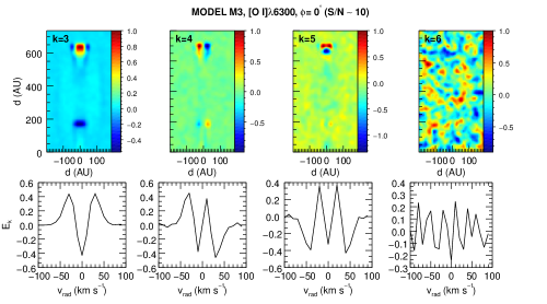
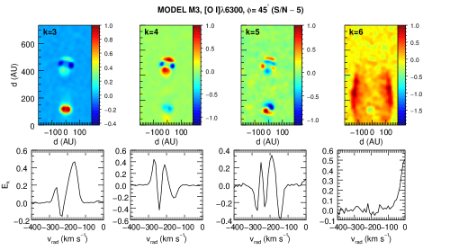
Figure 19.— Sequence from the third (left) to the sixth (right) tomogram and eigenspectra for M3 model and [O I]$\lambda$6300 emission line with a background noise. The two topmost panels are for S/N $\sim 10$ and $\phi=0^{\circ}$ and the bottommost ones are for S/N $\sim 5$ and $\phi=45^{\circ}$. The contribution to the variance is mainly dominated by noise fluctuation in high order eigenvectors.

References

- Anderson et al. (2003) Anderson, J.M., Li, Z.-Y., Krasnopolsky, R. et al. 2003, ApJ, 590, L107
- Bacciotti (2004) Bacciotti, F. 2004, Ap&SS, 293, 37
- Bacciotti et al. (2002) Bacciotti, F., Ray, T.P., Mundt, R. et al. 2002, ApJ, 576, 222
- Bacciotti et al. (2003) Bacciotti, F., Ray, T.P., Eislöffel, J. et al. 2003, Ap&SS, 287, 3
- Bacciotti et al. (2004) Bacciotti, F., Ray, T.P., Coffey, D. et al. 2004, Ap&SS, 292, 651
- Blandford & Payne (1982) Blandford, R.D., & Payne, D.G. 1982, MNRAS, 199, 1982
- Brunt, Heyer & Mac Low (2009) Brunt, C.M., Heyer, M.H. & Mac Low, M.-M. 2009, A&A, 504, 883
- Cabrit et al. (2006) Cabrit, S., Pety, J., Pesenti, N., et al. 2006, A&A, 452, 897
- Cai et al. (2008) Cai, M. J., Shang, H., Lin, H.-H., & Shu, F. H. 2008, ApJ, 672, 489
- Carrol, Frank & Blackman (2010) Carrol, J.A., Frank, A. & Blackman, E.G. 2010, ApJ, 722, 145
- Casse & Ferreira (2000a) Casse, F., & Ferreira, J. 2000a, A&A, 353, 1115
- Casse & Ferreira (2000b) Casse, F., & Ferreira, J. 2000b, A&A, 361, 1178
- Chrysostomou, Lucas & Hough (2007) Chrysostomou,A., Lucas, P.W., & Hough, J.H. 2007, Nature, 450, 71
- Cerqueira et al. (2015) Cerqueira, A.H., Vasconcelos, M.J., Raga, A.C. et al. 2015, AJ, 149, 98
- Cerqueira et al. (2006) Cerqueira, A.H., Velázquez, P.F., Raga, A.C. et al. 2006, A&A, 448, 2006
- Codella et al. (2007) Codella, C., Cabrit, S., Gueth, F., et al. 2007, A&A, 462, L53
- Coffey et al. (2004) Coffey, D., Bacciotti, F., Woitas, J., et al. 2004, ApJ, 604, 758
- Coffey et al. (2007) Coffey, D., Bacciotti, F., Ray, T.P., et al. 2007, ApJ, 663, 350
- Coffey, Bacciotti & Podio (2008) Coffey, D., Bacciotti, F., & Podio, L. 2008, ApJ, 689, 1112
- Coffey et al. (2011) Coffey, D., Bacciotti, F., Chrysostomou, A., et al. 2011, A&A, 526, 40
- Coffey et al. (2012) Coffey, D., Rigliaco, E., Bacciotti, F. et al. 2012, ApJ, 749, 139
- Coffey et al. (2015) Coffey, D., Dougados, C., Cabrit, S. et al. 2015, ApJ, 804, 2
- Correia et al. (2009) Correia, S., Zinnecker, H., Ridgway, S.T., et al 2009, A&A, 505, 673
- Davis et al. (2000) Davis, C.J., Berndsen, A., Smith, M.D., et al. 2000, MNRAS, 314, 241
- Dougados et al. (2003) Dougados, C., Cabrit, S., Lopez-Martin, L. et al. 2003, Ap&SS, 287, 135
- Dougados et al. (2004) Dougados, C., Cabrit, S., Ferreira, J. et al. 2004, Ap&SS, 292, 643
- Fendt (2011) Fendt, C. 2011, ApJ, 737, 43
- Ferreira (1997) Ferreira, J. 1997, A&A, 319, 340
- Ferreira (2008) Ferreira, J. 2008, New Astronomy Review, 52, 2008
- Ferreira, Dougados & Cabrit (2006) Ferreira, J., Dougados, C., & Cabrit, S. 2006, A&A, 453, 785
- Hartmman (2008) Hartmman, L. 2008, in Accretion Process in Star Formation, Cambridge University Press (2nd Edition)
- Heyer & Schloerb (1997) Heyer, M.H. & Schloerb, F.P. 1997, ApJ, 475, 173
- Kenyon, Dobrzycka & Hartmann (1994) Kenyon, S.J., Dobrzycka, D., & Hartmann, L. 1994, AJ, 108, 1872
- Krasnopolsky, Li & Blandford (2003) Krasnopolsky, R., Li, Z.-Y., & Blandford, R.D. 2003, ApJ, 595, 631
- Malyshev (2012) Malyshev, D. 2012, arXiv:1202.1034
- Melnikov et al. (2009) Melnikov, S.Yu, Eislöffel, J., Bacciotti, F., et al. 2009, A&A, 506, 763
- Menezes et al. (2014) Menezes, R. B., Steiner, J. E., & Ricci, T. V. 2014, ApJ, 796, LL13
- Mundt et al. (1990) Mundt, R., Buehrke, T., Solf, J., Ray, T. P., & Raga, A. C. 1990, A&A, 232, 37
- Pesenti et al. (2004) Pesenti, N., Dougados, N., Cabrit, S. et al. 2004, A&A, 416, L9
- Pety et al. (2006) Pety, J., Gueth, F., Guilloteau, S., & Dutrey, A. 2006, A&A, 458, 841
- Pudritz (2004) Pudritz, R.E. 2004, Ap&SS, 292, 471
- Pudritz & Norman (1983) Pudritz, R.E., & Norman, M.L., 1983, ApJ, 274, 677
- Pudritz & Norman (1986) Pudritz, R.E., & Norman, M.L., 1986, ApJ, 301, 571
- Pudritz et al. (2012) Pudritz, R.E., Hardcastle, M.J., & Gabuzda, D.C., 2012, Space Science Reviews, 169, 27
- Raga et al. (2000) Raga, A. C., Navarro-González, R., & Villagrán-Muniz, M. 2000, RMxAA, 36, 67
- Ricci et al. (2011) Ricci, T., Steiner, J., & Menezes, R.B. 2011, ApJ, 734, L10
- Sauty et al. (2012) Sauty, C., Cayatte, V., Lima, J.J.G., et al. 2012, ApJ, 759, L1
- Smith & Rosen (2007) Smith, M.D., & Rosen, A., 2007, MNRAS, 378, 691
- Solf & Böhm (1993) Solf, J., & Böhm, K.H. 1993, ApJ, 410, L31
- Spruit (1996) Spruit, H.C. 1996, in Evolutionary Processes in Binary Stars (R.A.M.J. Wijers et al., eds.), pp. 249-286, Kluwer, Dordrecht
- Staff et al. (2010) Staff, J.E., Niebergal, B.P., Ouyed, R., et al. 2010, ApJ, 722, 1325
- Steiner et al. (2009) Steiner, J., Menezes, R.B., Ricci, T. et al. 2009, MNRAS, 396, 788
- Testi et al. (2002) Testi, L., Bacciotti, F., Sargent, A.I. et al. 2002, A&A, 394, L31
- Vasconcelos et al. (2005) Vasconcelos, M.J., Cerqueira, A.H., Plana, H., Raga, A.C., & Morisset, C. 2005, AJ, 130, 1707