Effective charge of cylindrical and spherical colloids immersed in an electrolyte: the quasi-planar limit

Abstract

We consider the non-linear Poisson-Boltzmann theory for a single cylindrical or spherical macro-ion in symmetric 1:1, together with asymmetric 1:2 and 2:1 electrolytes. We focus on the regime where $\kappa a$, the ratio of the macro-ion radius $a$ over the inverse Debye length in the bulk electrolyte, is large. Analyzing the structure of the analytical expansion emerging from a multiple scale analysis, we uncover a hidden structure for the electrostatic potential. This structure, which appears after a heuristic resummation, suggests a new and convenient expansion scheme that we present and work out in detail. We show that novel exact results can thereby be obtained, in particular pertaining to effective charge properties, in complete agreement with the direct numerical solution to the problem.

I Introduction

Colloidal suspensions are composed of large and often highly charged macromolecules (macro-ions or colloids), immersed in an electrolyte (“salt”) solution of mobile, positively or negatively charged micro-ions. These micro-ions move in a solvent that is in a first approximation regarded as a medium of uniform dielectric permittivity. The system as a whole is assumed to be in thermal equilibrium at some inverse temperature $\beta=1/(k_{\rm B}T)$.

In the 1920s, Debye and Hückel (DH) Debye proposed a linearized mean-field description of the bulk thermodynamics of Coulomb fluids which is adequate in the high-temperature region $\beta\to 0$. Some years earlier, Gouy Gouy10 and Chapman Chapman13 had established the nonlinear Poisson-Boltzmann (PB) mean-field treatment of the electric double layer, which served as a basis for the DVLO theory of colloidal interactions Verwey48 .

A simple framework for studying the thermodynamics of colloidal suspensions at finite density is provided by the cell model Belloni98 ; Hansen00 ; Lukatsky01 ; Levin02 . If however the concentration of colloids in the system is very low, in the first approximation one can ignore their mutual interaction and consider the so-called infinite dilution limit. Colloids can be then studied as isolated mesoscopic objects of a given shape and bare charge, situated in a charged solution. This will be the viewpoint adopted here and for simplicity, we will address the homogeneous dielectric case with the dielectric permittivity of the colloid $\epsilon^{\prime}$ equal to that of the solvent $\epsilon$ (no electrostatic image charges).

The concept of (effective) charge renormalization, introduced by Alexander et al Alexander84 in the context of the PB cell model is simple to define in the infinite dilution limit: the renormalized/effective charge follows from the far-potential induced in the electrolyte Diehl01 ; Trizac02 ; Bocquet02 . At large distances from a charged body with bare charge $Q_{\rm bare}$, the electrostatic potential takes the same form as that obtained within the linearized DH theory, with a modified prefactor $Q_{\rm eff}$ which embodies the nonlinear effects of the PB theory, or of an approach which goes beyond the mean-field description. Within the nonlinear PB approach, $Q_{\rm eff}\simeq Q_{\rm bare}$ for low values of $|Q_{\rm bare}|$ while $Q_{\rm eff}$ saturates to a finite constant when $|Q_{\rm bare}|\to\infty$. In general, one expects that $|Q_{\rm eff}|\ll|Q_{\rm bare}|$ as a consequence of the nonlinear screening effect of the electric double layer around a colloid. For a monovalent 1:1 electrolyte the effective charge is indeed always smaller than the bare one. This is no longer true for asymmetric electrolytes which exhibit an overshooting effect Tellez04 : there exists a (rather small) interval of $Q_{\rm bare}$ where $|Q_{\rm eff}|\geq|Q_{\rm bare}|$.

Although the definition of an effective charge is unambiguous within the nonlinear PB theory, it is not clear whether the far-potential behaves like the DH one in an exact description which goes beyond the mean-field assumption. The two-dimensional symmetric Coulomb gas of pointlike $\pm q$ charges, interacting via the logarithmic Coulomb potential, is integrable in the whole interval of couplings $0\leq\Gamma\equiv\beta q^{2}<2$ where oppositely charged couples of charges do not collapse Samaj00 . The concept of renormalized charge has been shown to be valid for a charged conductor wall Samaj05a , a pointlike guest charge Samaj05b and for a guest charge with a small hard core Tellez05 ; Samaj06 which permits one to go beyond the stability threshold. It is interesting that for a guest charge with a small hard core at a finite temperature Samaj06 , $Q_{\rm eff}$ turns out to be a non-monotonous function of $Q_{\rm bare}$; the same phenomenon was observed also in Monte-Carlo Groot91 and molecular-dynamics Diehl04 simulations of the salt-free cell model. Moreover, as $Q_{\rm bare}$ goes to infinity, the effective charge does not saturate to a value but oscillates between two extreme (minimal and maximal) values.

In this paper, we restrict ourselves to the definition of the effective charge within the nonlinear PB theory. For a charged infinite plane, one can obtain explicit results for the symmetric 1:1 and asymmetric 1:2 and 2:1 electrolytes Gouy10 . For other asymmetric two-component electrolytes, the solution can be constructed implicitly, see a short review Tellez11 . Realistic macro-ions are usually modeled as curved objects, namely cylinders or spheres of a given radius $a$. For such systems, the functional relation between $Q_{\rm eff}$ and $Q_{\rm bare}$ depends, besides the salt content, also on the dimensionless parameter $\kappa a$ where $\kappa$ is the inverse Debye (correlation) length of micro-particles. Two limiting cases are studied:

• If $\kappa a\ll 1$, the analysis is difficult due to the counter-ion evaporation phenomenon, that may in the no salt limit be complete for spheres, or partial for cylinders, see Ramanathan83 and Ramanathan88 . Yet, the cylindrical PB equation is Painlevé integrable for the symmetric 1:1 and asymmetric 2:1 and 1:2 electrolytes. This enables one to construct systematically the non-analytical $\kappa a$-expansion of the effective charge Tellez06 .

• If $\kappa a\gg 1$, the colloid radius is large compared to the Debye length $\kappa^{-1}$ and the plane geometry is a good reference for finding $1/(\kappa a)$ expansions of the effective charge. Shkel et al Shkel00 constructed an asymptotic large-distance expansion of cylindrical and spherical PB equations for the symmetric 1:1 electrolyte. Using the method of multiple scales, they were able to derive the first two terms of the $1/(\kappa a)$ expansion of the electric potential. Based on this work, analytical approximations were developed in Ref. Aubouy03 for the symmetric 1:1 electrolyte and in Ref. Tellez04 for the asymmetric 2:1 and 1:2 electrolytes.

The present paper concentrates on the large $\kappa a$ limit, constructing expansions in $1/(\kappa a)$ for the effective charge of cylindrical and spherical colloids. The multiple-scale method applied in the previous Refs. Shkel00 ; Aubouy03 ; Tellez04 is laborious and in practice does not allow to go to high orders of the $1/(\kappa a)$ expansions. However, inspecting the structure of these results suggests some re-summation can be performed, which in turn strongly points to a novel re-parametrization of the electric potential. Pushing further this idea, it appears that the algebra is conducive to a much easier derivation of the $1/(\kappa a)$ expansions. For the cylindrical geometry especially, the formulation ends up with a representation of each expansion order in terms of finite polynomials, which enables one to construct expansions to arbitrary high orders. As concerns the spherical geometry, we were able to go one order beyond the results of Shkel00 ; Aubouy03 ; Tellez04 ; as a by product of the analysis, a divergence problem for higher-order terms indicates the change of the analytic behaviour of the expansion. For both cylindrical and spherical geometries and the three types of electrolytes (1:1, 1:2 and 2:1), the obtained analytical results for the coefficients of the $1/(\kappa a)$ series expansions are tested against numerical resolutions.

The article is organized as follows. In Sec. II, we introduce basic formulae and definitions which are used throughout the paper. It is elementary and may be skipped by the reader familiar with the subject. The large-distance formalism of Shkel et al Shkel00 and the ensuing possible re-parametrization of the PB potential, are then explained in Sec. III. Our approach is presented for 1:1 electrolytes in Sec. IV, for 2:1 electrolytes in Sec. V and for 1:2 electrolytes in Sec. VI. A brief recapitulation and concluding remarks are given in Sec. VII.

II Basic formalism

II.1 Microscopic models

In this paper, we shall consider the infinite dilution limit of colloids in suspensions, namely a unique colloid immersed in an infinite electrolyte solution. The system is formulated in the three-dimensional (3D) Euclidean space rque50 . Three colloidal shapes are of interest:

• The planar case, when the colloid occupies the half-space $z\leq 0$. The surface at $z=0$ bears fixed surface charge density $\sigma e$, where $e$ denotes the elementary charge and $\sigma$ has dimension $[{\rm length}]^{-2}$; without any loss of generality we assume that $\sigma>0$.

• The cylindrical geometry, when the colloid corresponds to an infinitely long cylinder of radius $a$, say along the $z$-axis, carrying a bare linear charge density $\lambda e$, $\lambda$ having dimension $[{\rm length}]^{-1}$. The system has a polar symmetry in the $(x,y)$ plane.

• The spherical geometry where the colloid is a sphere of radius $a$ with center localized at the origin ${\bf 0}$ and carrying a bare charge $Ze$. $Z$ is dimensionless and the system is radially symmetric.

The space outside the macro-ion is filled by an infinite electrolyte solution. In general, it consists of $M$ $(=2,3,\ldots)$ types of mobile (pointlike) micro-ions $\nu=1,2,\ldots,M$ with positive or negative charges $\{q_{\nu}e\}$, where $|q_{\nu}|$ is the valence of $\nu$-species. The charged particles are immersed in a solvent which is a medium of uniform dielectric permittivity $\epsilon$ (in Gauss units, $\epsilon\simeq 80$ for water). They interact with each other and with the charged colloid surface via the standard Coulomb potential $v({\bf r})=1/(\epsilon|{\bf r}|)$, which is the solution of the 3D Poisson equation

$$\Delta v({\bf r})=-\frac{4\pi}{\epsilon}\delta({\bf r}).$$ (2.1)

The system is in thermal equilibrium at the inverse temperature $\beta=1/(kT)$; we denote by $\langle\cdots\rangle$ the statistical averaging over a thermodynamic ensemble. It is useful to introduce the so-called Bjerrum length $l_{\rm B}\equiv\beta e^{2}/\epsilon$, i.e. the distance at which two unit charges interact with thermal energy $kT$. The macroscopic (i.e. thermodynamically averaged over all possible particle configurations) density of $\nu$-species at point ${\bf r}$ is defined by $n_{\nu}({\bf r})=\langle\hat{n}_{\nu}({\bf r})\rangle$, where $\hat{n}_{\nu}({\bf r})=\sum_{i}\delta({\bf r}-{\bf r}_{i})\delta_{\nu,\nu_{i}}$; $i$ numerates the particles of species $\nu_{i}$ at spatial positions ${\bf r}_{i}$, $\delta$ denotes Dirac/Kronecker delta function/symbol and the hat in $\hat{n}$ means “microscopic” (i.e. for a given particle configuration). The charge density at point ${\bf r}$ is given by

$$\rho({\bf r})=\langle\hat{\rho}({\bf r})\rangle,\qquad\hat{\rho}({\bf r})=\sum_{\nu}\hat{n}_{\nu}({\bf r})q_{\nu}e.$$ (2.2)

At large distances from an isolated colloid, i.e. in the bulk, the species number densities become homogeneous, $n_{\nu}({\bf r})=n_{\nu}$, and the requirement of the bulk electroneutrality is equivalent to

$$\rho({\bf r})=\rho=\sum_{\nu}n_{\nu}q_{\nu}e=0.$$ (2.3)

II.2 Poisson-Boltzmann equation

For a given charge density profile $\rho({\bf r}^{\prime})$, the mean electrostatic potential $\psi$ at point ${\bf r}$ is given by $\psi({\bf r})=\int{\rm d}{\bf r}^{\prime}\,v(|{\bf r}-{\bf r}^{\prime}|)\rho({\bf r}^{\prime})$. The potential satisfies a counterpart of the Poisson equation (2.1),

$$\Delta\psi({\bf r})=-\frac{4\pi}{\epsilon}\rho({\bf r}).$$ (2.4)

In the microscopic picture, the energy of an $\nu$-particle at point ${\bf r}$ can be expressed in terms of the microscopic potential $\hat{\psi}({\bf r})$ as $q_{\nu}e\hat{\psi}({\bf r})$ and the probability of finding the particle at ${\bf r}$ is proportional to the Boltzmann factor $\exp[-\beta q_{\nu}e\hat{\psi}({\bf r})]$. In a mean-field approach, one adopts this microscopic relation to the corresponding macroscopic values, $n_{\nu}({\bf r})=n_{\nu}\exp[-\beta q_{\nu}e\psi({\bf r})]$; the normalization by the bulk value is consistent with the assumption that $\psi({\bf r})$ and its derivatives vanish in the bulk. This relation is exact in the high-temperature limit and only approximative for a finite temperature comment66 . Considering it in the Poisson Eq. (2.4), one obtains a self-consistent PB equation for the mean electrostatic potential:

$$\Delta\psi({\bf r})=-\frac{4\pi e}{\epsilon}\sum_{\nu}n_{\nu}q_{\nu}\exp[-\beta q_{\nu}e\psi({\bf r})].$$ (2.5)

In terms of the reduced potential $\phi({\bf r})\equiv\beta e\psi({\bf r})$ and the inverse Debye length $\kappa=\sqrt{4\pi l_{\rm B}\sum_{\nu}n_{\nu}q_{\nu}^{2}}$, the PB equation can be rewritten as

$$\Delta\phi({\bf r})=-\frac{\kappa^{2}}{\sum_{\nu}n_{\nu}q_{\nu}^{2}}\sum_{\nu}n_{\nu}q_{\nu}{\rm e}^{-q_{\nu}\phi({\bf r})}.$$ (2.6)

All studied geometries are effectively one-dimensional problems. Let $r$ be the distance from the plane in the planar case, the distance $\sqrt{x^{2}+y^{2}}$ from the cylinder axis $z$ or the distance $\sqrt{x^{2}+y^{2}+z^{2}}$ from the sphere center. The Laplacian for such symmetric case can be written as

$$\Delta\to\frac{1}{r^{\alpha}}\frac{\rm d}{{\rm d}r}\left(r^{\alpha}\frac{\rm d}{{\rm d}r}\right)=\frac{{\rm d}^{2}}{{\rm d}r^{2}}+\frac{\alpha}{r}\frac{\rm d}{{\rm d}r},$$ (2.7)

where $\alpha=0$ for the planar case, $\alpha=1$ for the cylindrical geometry and $\alpha=2$ for the spherical geometry. The corresponding second-order differential equation (2.6) has to be supplemented by two boundary conditions (BCs), one at the contact with the colloid and the regularity one at an infinite distance from the colloid. The best way to derive these BCs is to consider the overall electroneutrality of the system.

• The planar case: Integrating the 1D Poisson equation

  $$\frac{{\rm d}^{2}\psi(r)}{{\rm d}r^{2}}=-\frac{4\pi}{\epsilon}\rho(r)$$ (2.8)

  over $r$ from $0$ to $\infty$, we get

  $$\psi^{\prime}(\infty)-\psi^{\prime}(0)=-\frac{4\pi}{\epsilon}\int_{0}^{\infty}{\rm d}r\,\rho(r).$$ (2.9)

  The requirement of the overall electroneutrality

  $$\sigma e+\int_{0}^{\infty}{\rm d}r\,\rho(r)=0$$ (2.10)

  then implies the couple of BCs for the reduced potential

  $$\phi^{\prime}(0)=-4\pi l_{\rm B}\sigma,\qquad\lim_{r\to\infty}\phi^{\prime}(r)=0.$$ (2.11)

• Cylindrical geometry: For a given charge density profile of particles at $r\geq a$, the electroneutrality condition reads as

  $$\lambda e+\int_{a}^{\infty}{\rm d}r\,2\pi r\rho(r)=0.$$ (2.12)

  Multiplying the 2D Poisson equation

  $$\frac{1}{r}\frac{\rm d}{{\rm d}r}\left(r\frac{{\rm d}\psi}{{\rm d}r}\right)=-\frac{4\pi}{\epsilon}\rho(r)$$ (2.13)

  by $r$ and integrating over $r$ from $a$ to $\infty$, the condition of overall electroneutrality is consistent with two BCs for the reduced potential

  $$a\phi^{\prime}(a)=-2l_{\rm B}\lambda,\qquad\lim_{r\to\infty}r\phi^{\prime}(r)=0.$$ (2.14)

• Spherical geometry: The electroneutrality condition reads

  $$Ze+\int_{a}^{\infty}{\rm d}r\,4\pi r^{2}\rho(r)=0.$$ (2.15)

  With regard to the 3D Poisson equation

  $$\frac{1}{r^{2}}\frac{\rm d}{{\rm d}r}\left(r^{2}\frac{{\rm d}\psi}{{\rm d}r}\right)=-\frac{4\pi}{\epsilon}\rho(r),$$ (2.16)

  the electroneutrality condition is equivalent to two BCs

  $$a^{2}\phi^{\prime}(a)=-l_{\rm B}Z,\qquad\lim_{r\to\infty}r^{2}\phi^{\prime}(r)=0.$$ (2.17)

II.3 Effective charge

The nonlinear PB equation (2.6) can be linearized by applying the expansion $\exp[-q_{\nu}\phi({\bf r})]\sim 1-q_{\nu}\phi({\bf r})$. With regard to the bulk electroneutrality condition (2.3), we arrive at the linear DH equation

$$\Delta\phi_{\rm DH}({\bf r})=\kappa^{2}\phi_{\rm DH}({\bf r}),$$ (2.18)

whose form does not depend on the particular composition of the electrolyte. This equation, supplemented by the appropriate boundary conditions, is solvable explicitly for all considered geometries.

The linearization of the potential Boltzmann factor is not adequate mainly in the neighbourhood of the colloid, where the potential is large. On the other hand, at asymptotically large distances from the colloid the potential is infinitesimally small and the linearization procedure is exact. We can say that the asymptotic PB solution satisfies the linear equation

$$\Delta\phi({\bf r})=\kappa^{2}\phi({\bf r}),\qquad|{\bf r}|\to\infty.$$ (2.19)

Comparing with the DH equation (2.18) we see that the asymptotic forms of the PB and DH solutions are equivalent, up to position-independent prefactors:

$$\phi_{\rm DH}(r)\mathop{\sim}_{r\to\infty}A_{DH}(Q)f(\kappa r),\qquad\phi(r)\mathop{\sim}_{r\to\infty}A(Q)f(\kappa r).$$ (2.20)

Here, the dependence of the $A$-prefactors on the thermodynamic parameters of the electrolyte like $\kappa a$ will not be explicitly indicated and $Q$ is the bare charge characteristics of the colloid (the surface charge density $\sigma e$ for the plane case $\alpha=0$, the line charge density $\lambda e$ for the cylinder $\alpha=1$ and the charge $Ze$ for the sphere $\alpha=2$).

The effective charge $Q_{\rm eff}$ is defined as a function of the bare charge $Q$ via the formula

$$A(Q)=A_{\rm DH}(Q_{\rm eff}).$$ (2.21)

In other words, $Q_{\rm eff}(Q)$ is the effective charge in the linear DH theory which reproduces the correct PB asymptotic behavior; $Q_{\rm eff}$ accounts for nonlinear effects, most prevalent close to the surface of the colloid. The nonlinear effects are negligible in the limit $Q\to 0$ and one expects that $Q_{\rm eff}(Q)\mathop{\sim}_{Q\to 0}Q$. In the opposite limit $Q\to\infty$ one anticipates that the saturation value of the effective charge

$$Q_{\rm eff}^{\rm sat}\equiv\lim_{Q\to\infty}Q_{\rm eff}(Q)$$ (2.22)

is finite.

Let us now assume that we know the prefactor $A(Q)$ and derive an explicit formula for the effective charge for each of the three geometries.

• The planar case: The solution of the DH equation

  $$\phi^{\prime\prime}_{\rm DH}(r)=\kappa^{2}\phi_{\rm DH}(r)$$ (2.23)

  with the BCs (2.11) takes the form

  $$\phi_{\rm DH}(r)=\frac{4\pi l_{\rm B}\sigma}{\kappa}{\rm e}^{-\kappa r}.$$ (2.24)

  Let us choose $A_{\rm DH}(\sigma)=4\pi l_{\rm B}\sigma/\kappa$ and $f(\kappa r)={\rm e}^{-\kappa r}$. Anticipating that the nonlinear PB potential behaves asymptotically as

  $$\phi(r)\mathop{\sim}_{r\to\infty}A(\sigma){\rm e}^{-\kappa r},$$ (2.25)

  using the prescription (2.21) the effective surface charge density $\sigma_{\rm eff}e$ depends on the bare one $\sigma e$ as follows

  $$\frac{4\pi l_{\rm B}}{\kappa}\sigma_{\rm eff}=A(\sigma).$$ (2.26)

• Cylindrical geometry: The linearized DH equation

  $$\phi^{\prime\prime}_{\rm DH}(r)+\frac{1}{r}\phi^{\prime}_{\rm DH}(r)=\kappa^{2}\phi_{\rm DH}(r)$$ (2.27)

  with the BCs (2.14) provides the solution

  $$\phi_{\rm DH}(r)=\frac{2\lambda l_{\rm B}}{\kappa aK_{1}(\kappa a)}K_{0}(\kappa r),\qquad r\geq a,$$ (2.28)

  where $K_{0}$ and $K_{1}$ are the modified Bessel functions. Since $K_{0}(\kappa r)\sim\sqrt{\pi/(2\kappa r)}{\rm e}^{-\kappa r}$ for asymptotically large $r$ we can choose

  $$A_{\rm DH}(\lambda)=\frac{\sqrt{2\pi}}{\kappa aK_{1}(\kappa a)}\lambda l_{\rm B},\qquad f(\kappa r)=\frac{1}{\sqrt{\kappa r}}{\rm e}^{-\kappa r}.$$ (2.29)

  The prefactor to the asymptotic behaviour of the full PB potential

  $$\phi(r)\mathop{\sim}_{r\to\infty}A(\lambda)\frac{1}{\sqrt{\kappa r}}{\rm e}^{-\kappa r}$$ (2.30)

  determines the dependence of the effective line charge density $\lambda_{\rm eff}e$ on the bare one $\lambda e$ as follows

  $$\lambda_{\rm eff}l_{\rm B}=\frac{1}{\sqrt{2\pi}}\kappa aK_{1}(\kappa a)A(\lambda).$$ (2.31)

• Spherical geometry: The linearized DH equation

  $$\phi^{\prime\prime}_{\rm DH}(r)+\frac{2}{r}\phi^{\prime}_{\rm DH}(r)=\kappa^{2}\phi_{\rm DH}(r)$$ (2.32)

  with the BCs (2.17) has the solution

  $$\phi_{\rm DH}(r)=\frac{Z\kappa l_{\rm B}}{1+\kappa a}\frac{1}{\kappa r}{\rm e}^{-\kappa(r-a)},\qquad r\geq a.$$ (2.33)

  It is natural to choose

  $$A_{\rm DH}(Z)=\frac{\kappa}{1+\kappa a}{\rm e}^{\kappa a}Zl_{\rm B},\qquad f(\kappa r)=\frac{1}{\kappa r}{\rm e}^{-\kappa r}.$$ (2.34)

  Taking into account the expected asymptotic behaviour of the PB potential

  $$\phi(r)\mathop{\sim}_{r\to\infty}A(Z)\frac{1}{\kappa r}{\rm e}^{-\kappa r},$$ (2.35)

  the formula for the effective charge $Z_{\rm eff}e$ as the function of the bare charge $Z$ reads as

  $$Z_{\rm eff}\frac{l_{\rm B}}{a}=\frac{1+\kappa a}{\kappa a}{\rm e}^{-\kappa a}A(Z).$$ (2.36)

  In other words, $Z_{\rm eff}$ is the value that should be plugged in the right-hand side of (2.33), so that the latter formula provides the correct far-field of the non-linear solution to the PB equation. By construction thus, $Z_{\rm eff}=Z$ when the PB theory is linearizable, which is the case for $Z\to 0$.

II.4 Explicit results for the planar case

The planar case is solvable explicitly only for specific types of two-component electrolytes.

• Symmetric 1:1 electrolyte. We have two types of particles with (reduced) positive $q_{1}=1$ and negative $q_{2}=-1$ charges. Denoting by $n$ the total particle number density, the requirement of the bulk electroneutrality is equivalent to $n_{1}=n_{2}=n/2$. The inverse Debye length is given by $\kappa=\sqrt{4\pi l_{\rm B}n}$. The corresponding PB equation

  $$\phi^{\prime\prime}(r)=\kappa^{2}\sinh\phi(r)$$ (2.37)

  has the explicit solution

  $$\phi(r)=2\ln\left[\frac{1+\frac{A(\sigma)}{4}{\rm e}^{-\kappa r}}{1-\frac{A(\sigma)}{4}{\rm e}^{-\kappa r}}\right]$$ (2.38)

  which indeed behaves at large $\kappa r$ as predicted by formula (2.25). The relation between $A$ and $\sigma$ is yielded by the BC (2.11) at $r=0$:

  $$A(\sigma)=\frac{8\pi l_{\rm B}\sigma}{\kappa}\frac{1}{1+\sqrt{1+\left(\frac{2\pi l_{\rm B}\sigma}{\kappa}\right)^{2}}}.$$ (2.39)

  In accordance with the relation (2.26), the effective charge density is given by

  $$\sigma_{\rm eff}=\frac{2\sigma}{1+\sqrt{1+\left(\frac{2\pi l_{\rm B}\sigma}{\kappa}\right)^{2}}}.$$ (2.40)

  It has the correct behaviour $\sigma_{\rm eff}\sim\sigma$ in the limit $\sigma\to 0$. In the saturation $\sigma\to\infty$ limit, we have

  $$\frac{4\pi l_{\rm B}}{\kappa}\sigma_{\rm eff}^{\rm sat}=4.$$ (2.41)

• Asymmetric 2:1 electrolyte. In this case, the positively charged coions to the surface have $q_{1}=2$ and the negatively charged counterions have $q_{2}=-1$. The bulk electroneutrality requires that $n_{1}=n/3$ and $n_{2}=2n/3$, where $n$ is the total particle number density. The inverse Debye length $\kappa=\sqrt{8\pi l_{\rm B}n}$. The PB equation

  $$\phi^{\prime\prime}(r)=\kappa^{2}\frac{1}{3}\left[{\rm e}^{\phi(r)}-{\rm e}^{-2\phi(r)}\right]$$ (2.42)

  has been solved by Gouy Gouy10 :

  $$\phi(r)=\ln\left[1+\frac{A(\sigma){\rm e}^{-\kappa r}}{\left(1-\frac{A(\sigma)}{6}{\rm e}^{-\kappa r}\right)^{2}}\right].$$ (2.43)

  The potential behaves at large $\kappa r$ as (2.25). The relation between $A$ and $\sigma$ follows from the BC (2.11) at $r=0$:

  $$\frac{4\pi l_{\rm B}\sigma}{\kappa}=\frac{36A(6+A)}{(6-A)(A^{2}+24A+36)}.$$ (2.44)

  From the three $A$-solutions of this cubic equation we take the one which goes to zero in the limit $\sigma\to 0$. In the saturation limit $\sigma\to\infty$, we have $A_{\rm sat}=6$ and therefore

  $$\frac{4\pi l_{\rm B}}{\kappa}\sigma_{\rm eff}^{\rm sat}=6.$$ (2.45)

• Asymmetric 1:2 electrolyte. Now the coions have $q_{1}=1$ and the bulk number density $n_{1}=2n/3$, while the counterions have $q_{2}=-2$ and $n_{2}=n/3$. As before, $\kappa=\sqrt{8\pi l_{\rm B}n}$. The PB equation

  $$\phi^{\prime\prime}(r)=\kappa^{2}\frac{1}{3}\left[{\rm e}^{2\phi(r)}-{\rm e}^{-\phi(r)}\right]$$ (2.46)

  has the explicit solution

  $$\phi(r)=-\ln\left[1-\frac{A(\sigma){\rm e}^{-\kappa r}}{\left(1+\frac{A(\sigma)}{6}{\rm e}^{-\kappa r}\right)^{2}}\right].$$ (2.47)

  The relation between $A$ and $\sigma$, following from the BC (2.11) at $r=0$, takes the form

  $$\frac{4\pi l_{\rm B}\sigma}{\kappa}=\frac{36A(6-A)}{(6+A)(A^{2}-24A+36)}.$$ (2.48)

  The physical $A$-solution goes to zero in the limit $\sigma\to 0$. In the saturation limit $\sigma\to\infty$, $A_{\rm sat}=6(2-\sqrt{3})$ is the smaller root of the quadratic equation $A^{2}-24A+36=0$ and we arrive at

  $$\frac{4\pi l_{\rm B}}{\kappa}\sigma_{\rm eff}^{\rm sat}=6(2-\sqrt{3}).$$ (2.49)

III An asymptotic expansion for 1:1 electrolyte

For the symmetric 1:1 electrolyte of total particle number density $n$ and $\kappa=\sqrt{4\pi l_{\rm B}n}$, the general PB equation for the electrostatic potential $\phi$ reads as

$$\phi^{\prime\prime}(x)+\frac{\alpha}{x}\phi^{\prime}(x)=\sinh\phi(x),$$ (3.1)

where $x=\kappa r$ is the reduced distance, $\alpha=1$ for the cylindrical colloid and $\alpha=2$ for the spherical colloid. In the paper Shkel00 , an asymptotic large-$x$ expansion of the potential has been obtained in the following form

$$\phi(x) = \frac{{\rm e}^{-x}}{x^{\alpha/2}}\left(A_{00}+\frac{A_{01}}{x}+\frac{A_{02}}{x^{2}}+\cdots\right)+$$

$$+\frac{{\rm e}^{-3x}}{x^{3\alpha/2}}\left(A_{10}+\frac{A_{11}}{x}+\frac{A_{12}}{x^{2}}+\cdots\right)+\cdots$$

$$+\frac{{\rm e}^{-(2j+1)x}}{x^{(2j+1)\alpha/2}}\left(A_{j0}+\frac{A_{j1}}{x}+\frac{A_{j2}}{x^{2}}+\cdots\right)+\cdots.$$

Here, $A_{00}\equiv A$ is the crucial prefactor to the leading large-distance asymptotic. The other prefactors $A_{jk}$ scale with $A$ like $A_{jk}=a_{jk}A^{2j+1}$, where the coefficients (numbers) $\{a_{jk}\}$ fulfill a rather complicated recursion which enables one to generate systematically the coefficients $\{a_{jk}\}$ with small values of the $(j,k)$ indices Shkel00 .

The first $j=0$ row of the asymptotic formula (III), which consists in the exponential ${\rm e}^{-x}$ multiplied by an infinite inverse-power-law series, corresponds to the linear DH approximation. The next rows are exponentially smaller and smaller corrections to the DH result.

For our purposes, it is more important to concentrate on columns. Let us introduce the new variable

$$t(x)=\frac{A}{4}\frac{{\rm e}^{-x}}{x^{\alpha/2}}$$ (3.3)

where $A$ (and thus $t$) implicitly depends on the bare charge ($\lambda$ or $Z$ depending on the geometry), and $\kappa a$; we shall usually omit in the notation these functional dependences or write only the relevant ones. In the BC, the first derivative of the potential is taken just at the surface of the colloid, i.e. at $x=\kappa a$. The value of $t$ is, in general, not small at the colloid surface, even in the limit of interest $\kappa a\to\infty$. Note that the given column differs from the previous one basically by the factor $1/x$. The corresponding surface factor $1/(\kappa a)$ is small in the limit $\kappa a\to\infty$. This permits one to generate a systematic expansion of the prefactor $A$ in $1/(\kappa a)$ powers by taking successively column by column.

The asymptotic expansion (III) can be rewritten in the variables $t$ and $1/x$ as follows

$$\phi(x)=\sum_{j,k=0}^{\infty}t^{2j+1}B_{jk}\frac{1}{x^{k}},$$ (3.4)

where the coefficients

$$B_{jk}\equiv\left(\frac{4}{A}\right)^{2j+1}A_{jk}$$ (3.5)

are the numbers which will be explicitly available for small values of $(j,k)$ indices.

We shall also need the asymptotic large-$x$ expansion of the modified Bessel functions

$$K_{\nu}(x)=\sqrt{\frac{\pi}{2x}}{\rm e}^{-x}\sum_{k=0}^{\infty}\frac{1}{(2x)^{k}}\frac{\Gamma(\frac{1}{2}+\nu+k)}{k!\Gamma(\frac{1}{2}+\nu-k)}$$ (3.6)

for $\nu=0,1$.

III.1 Cylindrical geometry

For the $\alpha=1$ cylindrical geometry, we have the parameter

$$t(x)=\frac{A(\lambda)}{4}\frac{{\rm e}^{-x}}{\sqrt{x}}.$$ (3.7)

The coefficients $B_{jk}$ with $j,k=0,1,2,3,4$ are summarized in Table 1.

a j a	k=0	k=1	k=2	k=3	k=4
0	4	$-\dfrac{1}{2}$	$\dfrac{9}{2^{5}}$	$-\dfrac{75}{2^{8}}$	$\dfrac{3675}{2^{13}}$
1	$\dfrac{4}{3}$	$-\dfrac{3}{2}$	$\dfrac{71}{2^{5}}$	$-\dfrac{3215}{3\times 2^{8}}$	$\dfrac{79521}{2^{13}}$
2	$\dfrac{4}{5}$	$-\dfrac{3}{2}$	$\dfrac{89}{2^{5}}$	$-\dfrac{1485}{2^{8}}$	$\dfrac{114071}{2^{13}}$
3	$\dfrac{4}{7}$	$-\dfrac{3}{2}$	$\dfrac{107}{2^{5}}$	$-\dfrac{1965}{2^{8}}$	$\dfrac{157237}{2^{13}}$
4	$\dfrac{4}{9}$	$-\dfrac{3}{2}$	$\dfrac{125}{2^{5}}$	$-\dfrac{2517}{2^{8}}$	$\dfrac{211275}{2^{13}}$

Table 1: Cylindrical geometry. The coefficients $B_{jk}$ $(j,k=0,1,2,3,4)$ appearing in (3.5) for the large-distance expansion (III) obtained in Ref. Shkel00 .

The first row of the table corresponds to the DH result (2.28). Indeed, writing in (2.28) the large-$x$ expansion of the modified Bessel function (3.6) with $\nu=0$, the corresponding coefficients are found to be

$$B_{0k}\equiv 4\frac{A_{0k}}{A}=2^{2-k}\frac{\Gamma(\frac{1}{2}+k)}{k!\Gamma(\frac{1}{2}-k)},$$ (3.8)

the first few of which read $4$, $-1/2$, $9/2^{5}$ etc.

In accordance with our strategy, let us consider the first column of Table 1. From the first few coefficients $B_{j0}$ we can “guess”

$$B_{j0}=\frac{4}{2j+1}$$ (3.9)

and suggest that this formula holds for all $j=0,1,\ldots$. If this is true, the potential (3.4) is given, in the leading $1/x^{0}$ order, by

$$\phi(x)=4\sum_{j=0}^{\infty}\frac{t^{2j+1}}{2j+1}=2\ln\left(\frac{1+t}{1-t}\right).$$ (3.10)

This result is identical to the planar one (2.38) under the only proviso that the cylindrical $t$ (3.7) differs from the corresponding planar function $A{\rm e}^{-x}/4$ by the factor $1/\sqrt{x}$.

We can go further and sum the contributions of the second column of Table 1 to determine the potential up to the $1/x$ order. We anticipate that

$$B_{01}=-\frac{1}{2},\qquad B_{j1}=-\frac{3}{2}\quad\mbox{for $j\geq 1$.}$$ (3.11)

The potential (3.4) is then given by

$$\phi(x) = 2\ln\left(\frac{1+t}{1-t}\right)-\frac{1}{2x}t-\frac{3}{2x}\frac{t^{3}}{1-t^{2}}$$ (3.12)

$$= 2\ln\left(\frac{1+t}{1-t}\right)-\frac{t(1+2t^{2})}{4x}\left(\frac{1}{1-t}+\frac{1}{1+t}\right).\phantom{aaa}$$

The $1/x$ correction consists of $1/(1-t)$ and $1/(1+t)$ terms. They arise naturally from a “renormalization ansatz”

$$\phi(x)=2\ln\left(\frac{1+f(x)}{1-f(x)}\right)$$ (3.13)

with

$$f(x)=t(x)\left\{1-\frac{1}{8x}[1+2t^{2}(x)]\right\}.$$ (3.14)

It is easy to verify that this ansatz coincides with the original equation (3.12) to the order $1/x$.

The guessing of the coefficients becomes harder when considering the next columns. In the following section, we shall show how to generate systematically the whole infinite series of coefficients in a straightforward way. At this stage, we restrict ourselves to the preliminary result (3.13), (3.14).

For the solution of type (3.13), the BC (2.14) at $r=a$ can be expressed as

$$-l_{\rm B}\lambda=2\kappa a\frac{f^{\prime}(\kappa a)}{1-f^{2}(\kappa a)}.$$ (3.15)

This relation determines the function $A(\lambda)$. In the saturation limit $\lambda\to\infty$ we have $f_{\rm sat}(\kappa a)=1$, as indicated by Eq. (3.15). Consequently,

$$t_{\rm sat}(\kappa a)\left\{1-\frac{1}{8\kappa a}[1+2t_{\rm sat}^{2}(\kappa a)]\right\}=1.$$ (3.16)

Performing the large-$\kappa a$ expansion in this formula, we obtain

$$t_{\rm sat}(\kappa a)=1+\frac{3}{8\kappa a}+\cdots\equiv\frac{A_{\rm sat}}{4}\frac{{\rm e}^{-\kappa a}}{\sqrt{\kappa a}},$$ (3.17)

where $A_{\rm sat}\equiv A(\lambda\to\infty)$. Using that

$$K_{1}(\kappa a)=\sqrt{\frac{\pi}{2\kappa a}}{\rm e}^{-\kappa a}\left(1+\frac{3}{8\kappa a}+\ldots\right),$$ (3.18)

the formula for the effective charge (2.31) implies that its saturation value has the large-$\kappa a$ expansion of the form

$$\lambda_{\rm eff}^{\rm sat}l_{\rm B} = \frac{1}{\sqrt{2\pi}}\kappa aK_{1}(\kappa a)A_{\rm sat}$$ (3.19)

$$= 2\kappa a+\frac{3}{2}+\cdots.$$

This result agrees with the previous finding of Ref. Aubouy03 .

III.2 Spherical geometry

For the $\alpha=2$ spherical geometry, we have

$$t(x)=\frac{A}{4}\frac{{\rm e}^{-x}}{x}.$$ (3.20)

The coefficients $B_{jk}$ with $j,k=0,1,2,3,4$ are summarized in Table 2.

a j a	k=0	k=1	k=2	k=3	k=4
0	4	0	0	0	0
1	$\dfrac{4}{3}$	$-2$	$\dfrac{7}{2}$	$-\dfrac{15}{2}$	$\dfrac{155}{2^{3}}$
2	$\dfrac{4}{5}$	$-2$	$\dfrac{14}{3}$	$-\dfrac{35}{3}$	$\dfrac{2327}{3^{2}\times 2^{3}}$
3	$\dfrac{4}{7}$	$-2$	$\dfrac{205}{3^{2}\times 2^{2}}$	$-\dfrac{863}{3^{3}\times 2}$	$\dfrac{40621}{3^{3}\times 2^{5}}$
4	$\dfrac{4}{9}$	$-2$	$\dfrac{2413}{5\times 3^{2}\times 2^{3}}$	$-\dfrac{90271}{5\times 3^{3}\times 2^{5}}$	$\dfrac{11313029}{5^{2}\times 3^{3}\times 2^{8}}$

Table 2: Spherical geometry. The coefficients $B_{jk}$ $(j,k=0,1,2,3,4)$ appearing in (3.5) for the large-distance expansion (III) obtained in Ref. Shkel00 .

The first row of the table corresponds to the DH result (2.28), namely $B_{0k}=4\delta_{0k}$. The first column of Table 2 is identical to the first one of Table 1, so that

$$B_{j0}=\frac{4}{2j+1}$$ (3.21)

and, in the leading $1/x^{0}$ order, the potential is given by

$$\phi(x)=2\ln\left(\frac{1+t}{1-t}\right).$$ (3.22)

Again, this result is identical to the planar one (2.38) if the planar $t$ is multiplied by $1/x$.

It is easy to guess the second column of Table 2:

$$B_{01}=0,\qquad B_{0j}=-2\quad\mbox{for $j\geq 1$.}$$ (3.23)

The potential (3.4) is then given by

$$\phi(x)=2\ln\left(\frac{1+t}{1-t}\right)-\frac{t^{3}}{x}\left(\frac{1}{1-t}+\frac{1}{1+t}\right).$$ (3.24)

The potential is transformable to the renormalized form of type (3.13) with

$$f(x)=t(x)\left[1-\frac{1}{2x}t^{2}(x)\right].$$ (3.25)

As before, the saturation limit $Z\to\infty$ corresponds to $f_{\rm sat}(\kappa a)=1$. Consequently,

$$t_{\rm sat}(\kappa a)\left[1-\frac{1}{2\kappa a}t_{\rm sat}^{2}(\kappa a)\right]=1.$$ (3.26)

The large-$\kappa a$ expansion of $t_{\rm sat}(\kappa a)$ then reads

$$t_{\rm sat}(\kappa a)=1+\frac{1}{2\kappa a}+\cdots\equiv\frac{A_{\rm sat}}{4}\frac{{\rm e}^{-\kappa a}}{\kappa a},$$ (3.27)

where $A_{\rm sat}\equiv A(Z\to\infty)$. The formula for the effective charge (2.36) then leads to

$$Z_{\rm eff}^{\rm sat}\frac{l_{\rm B}}{a} = \frac{1+\kappa a}{\kappa a}{\rm e}^{-\kappa a}A_{\rm sat}$$ (3.28)

$$= 4\kappa a+6+\cdots$$

which coincides with the finding of Ref. Aubouy03 . It is instructive to compute the corresponding effective surface charge $\sigma_{\rm eff}^{\rm sat}=Z_{\rm eff}^{\rm sat}/(4\pi a^{2})$ and likewise for the cylinder, $\sigma_{\rm eff}^{\rm sat}=\lambda_{\rm eff}^{\rm sat}/(2\pi a)$. In doing so, it appears that Eq. (3.28) and Eq. (3.19) bear the same information. Indeed, introducing the curvature ${\cal C}=1/a$ for cylinders and ${\cal C}=2/a$ for spheres, both can be written, when phrased in terms of the effective surface charge, as

$$\sigma_{\rm eff}^{\rm sat}\,=\,\frac{\kappa}{\pi l_{\rm B}}\left(1+\frac{3\,\cal C}{4\,\kappa}\right).$$ (3.29)

To dominant order, that is when ${\cal C}=0$, we recover as expected the planar result of Eq. (2.41). This suggests that to dominant plus sub-dominant order, the effective charge only depends on the curvature, irrespective of further geometrical details rque1 . We shall see that this “universality” is broken by higher order terms in ${\cal C}^{2}$.

IV General formalism for 1:1 electrolyte

The above section motivates us to search for the potential $\phi(x)$ in the ansatz form (3.13) which is nothing but the redefinition of the potential in terms of a new function $f(x)$ with simpler expansion property, as we will see later. Inserting the ansatz (3.13) into the PB equation (3.1), we obtain after some simple algebra the following differential equation for the $f$-function:

$$\left[f^{\prime\prime}(x)+\frac{\alpha}{x}f^{\prime}(x)-f(x)\right]\left[1-f^{2}(x)\right]$$

$$-2f(x)\left[f(x)+f^{\prime}(x)\right]\left[f(x)-f^{\prime}(x)\right] = 0.$$ (4.1)

With regard to the results of the preceding section, we expect that the $f$-function can be written as

$$f(x)=tg(x),$$ (4.2)

where the $x$-dependent function $t$ is defined in (3.3) and the $g$-function is expected to have the following large-$x$ expansion

$$g(x)=1+\sum_{k=1}^{\infty}\frac{1}{x^{k}}g_{k}(t).$$ (4.3)

In the DH limit $t\to 0$, $f$ is going to 0 as well and from (3.13) we can write that $\phi(x)\sim 4f(x)$. Using the original expansion (3.4), we identify

$$g_{k}(0)=\frac{B_{0k}}{4}\qquad\mbox{for all $k=1,2,\ldots$.}$$ (4.4)

From the definition of $t$ in Eq. (3.3), we have that

$$t^{\prime}(x)=-\left(1+\frac{\alpha}{2x}\right)t,\qquad t^{\prime\prime}(x)=\left[\left(1+\frac{\alpha}{2x}\right)^{2}+\frac{\alpha}{2x^{2}}\right]t.$$ (4.5)

Inserting the representation (4.2) into Eq. (4.1) and using these relations, we obtain the differential equation for the $g$-function:

$$\left[g^{\prime\prime}(x)-2g^{\prime}(x)+\frac{\alpha(2-\alpha)}{4x^{2}}g(x)\right]\left[1-t^{2}g^{2}(x)\right]$$

$$-2t^{2}g(x)\left[g^{\prime}(x)-\frac{\alpha}{2x}g(x)\right]\left[\left(2+\frac{\alpha}{2x}\right)g(x)-g^{\prime}(x)\right] = 0.$$

We emphasize that a prime here means the total derivative with respect to $x$, including the function $t(x)$. Like for instance, within the representation (4.3) we have

$$g^{\prime}(x)=-\sum_{k=1}^{\infty}\frac{1}{x^{k+1}}\left[kg_{k}(t)+\frac{\alpha}{2}tg^{\prime}_{k}(t)\right]-\sum_{k=1}^{\infty}\frac{1}{x^{k}}tg^{\prime}_{k}(t)$$ (4.7)

and so on. The point is that the total derivative with respect to $x$ keeps the power-law expansion in $1/x$ where each term is multiplied by a function depending on $t$ only. This two-scale method permits us to determine recursively the functions $\{g_{k}(t)\}$. Setting to zero the coefficient to $1/x$, we obtain a differential equation for $g_{1}(t)$, supplemented by the BC $g_{1}(0)=B_{01}/4$ deduced from (4.4). Setting to zero the coefficient to $1/x^{2}$, we obtain a differential equation for $g_{2}(t)$ which involves also the known function $g_{1}(t)$, supplemented by the BC $g_{2}(0)=B_{02}/4$, etc.

IV.1 Cylindrical geometry

We start with the cylindrical geometry for which $\alpha=1$. The BC (4.4) implies

$$g_{k}(0)=\frac{1}{2^{k}}\frac{\Gamma(\frac{1}{2}+k)}{k!\Gamma(\frac{1}{2}-k)}$$ (4.8)

for all $k=1,2,\ldots$.

Setting to zero the coefficient to $1/x$ in (LABEL:gequations), $g_{1}(t)$ must obey the differential equation

$$t(1-t^{2})g_{1}^{\prime\prime}(t)+(3+t^{2})g_{1}^{\prime}(t)+2t=0.$$ (4.9)

The general solution of this equation, obtained by using the ‘variation of constants’ method, reads as

$$g_{1}(t)=c_{1}+c_{2}t^{2}-(1+4c_{2})\left(\ln t+\frac{1}{4t^{2}}\right).$$ (4.10)

The integration constant $c_{2}$ is determined by the regularity of $g_{1}(t)$ as $t\to 0$ as follows $c_{2}=-1/4$. The BC $g_{1}(0)=-1/8$ leads to $c_{1}=-1/8$. The consequent

$$g_{1}(t)=-\frac{1}{8}\left(1+2t^{2}\right)$$ (4.11)

is in full agreement with the previous result (3.14).

To find $g_{2}(t)$, we set to zero the coefficient to $1/x^{2}$ in (LABEL:gequations) which, together with the knowledge of $g_{1}(t)$, implies

$$t(1-t^{2})g_{2}^{\prime\prime}(t)+(3+t^{2})g_{2}^{\prime}(t)+\frac{t}{4}(2t^{4}-6t^{2}-15)=0.$$ (4.12)

The general solution of this differential equation is

$$g_{2}(t)=c_{1}+c_{2}t^{2}+\frac{t^{4}}{16}+\left(\frac{15}{8}-4c_{2}\right)\left(\ln t+\frac{1}{4t^{2}}\right).$$ (4.13)

The regularity of $g_{2}(t)$ at $t=0$ implies $c_{2}=15/32$ and the BC $g_{2}(0)=9/128$ fixes $c_{1}=9/128$. Thus we arrive at

$$g_{2}(t)=\frac{3^{2}}{2^{7}}+\frac{3\times 5}{2^{5}}t^{2}+\frac{1}{4^{2}}t^{4}.$$ (4.14)

In the same way, e.g. by using the symbolic language Mathematica, we get

$$g_{3}(t) = -\frac{3\times 5^{2}}{2^{10}}-\frac{163\times 3}{2^{9}}t^{2}-\frac{29}{2^{7}}t^{4}-\frac{1}{4^{3}}t^{6},$$ (4.15)

$$g_{4}(t) = \frac{3\times(5\times 7)^{2}}{2^{15}}+\frac{3\times 53\times 59}{2^{12}}t^{2}+\frac{3^{4}\times 17}{2^{11}}t^{4}$$ (4.16)

$$+\frac{43}{2^{9}}t^{6}+\frac{1}{4^{4}}t^{8},$$

etc. In general, $g_{k}(t)$ with $k=1,2,\ldots$ turns out to be a finite polynomial of the $k$th order in the variable $t^{2}$. This special and convenient property of the $g_{k}$-functions is present exclusively for the case of the cylindrical geometry and the symmetric $1:1$ electrolyte.

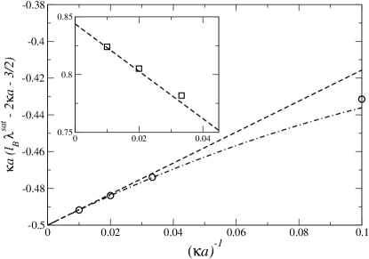
Figure 1: Asymptotic expansion plots for cylinders in a 1:1 salt. The main graph shows $\kappa a(\lambda_{\rm eff}^{\rm sat}l_{B}-2\kappa a-3/2)$ as a function of $1/(\kappa a)$. The dashed linear curve is for the first order correction predicted by Eq. (4.18), $-1/2+27/(32\kappa a)$, while the parabolic dot-dashed curve is for $-1/2+27(\kappa a)^{-1}/32-131(\kappa a)^{-2}/64$. The symbols correspond to the saturated effective charge obtained from the numerical solution of Eq. (3.1) with $\alpha=1$, and have been computed for $\kappa a=10$, 30, 50 and 100, as can be read on the $x$-axis. Inset : $(\kappa a)^{2}[\lambda_{\rm eff}^{\rm sat}l_{B}-2\kappa a-3/2-0.5/(\kappa a)]$ versus $1/(\kappa a)$. The linear dashed curve displays the prediction of Eq. (3.1) for the quantity of interest, namely $27/32-131(\kappa a)^{-1}/64$.

Having $f(x)$ (4.2) with $g(x)$ (4.3) truncated say at $k=4$, the crucial function $A(\lambda)$ is again determined by the relation (3.15). In the saturation limit $\lambda\to\infty$, the requirement $f_{\rm sat}(\kappa a)=1$ implies the iteratively generated large-$\kappa a$ expansion

$$t_{\rm sat}(\kappa a) = 1+\frac{3}{2^{3}}\frac{1}{\kappa a}-\frac{5\times 7}{2^{7}}\frac{1}{(\kappa a)^{2}}+\frac{53\times 3^{2}}{2^{10}}\frac{1}{(\kappa a)^{3}}$$ (4.17)

$$-\frac{7369\times 5}{2^{15}}\frac{1}{(\kappa a)^{4}}+\cdots$$

which goes beyond the previous one (3.17). Using the connection (3.19), the corresponding saturation value of the effective charge exhibits the large-$\kappa a$ expansion of the form

$$\lambda_{\rm eff}^{\rm sat}l_{\rm B} = 2\kappa a+\frac{3}{2}-\frac{1}{2}\frac{1}{\kappa a}+\frac{27}{32}\frac{1}{(\kappa a)^{2}}$$ (4.18)

$$-\frac{131}{64}\frac{1}{(\kappa a)^{3}}+O\left(\frac{1}{(\kappa a)^{4}}\right).$$

Notice that in spite of the complicated large-$\kappa a$ expansion of $t_{\rm sat}(\kappa a)$, the corresponding expression for $\lambda_{\rm eff}^{\rm sat}$ is relatively simple. The numerical checks of the coefficients to the $1/(\kappa a)$, $1/(\kappa a)^{2}$, $\ldots$ terms are presented in Fig. 1. Such a comparison poses the difficulty that the effective charge $\lambda_{\rm eff}$ be known with high precision in the limit where the bare charge $\lambda$ diverges. To this end, the Poisson-Boltzmann equation (3.1) is solved numerically for a series of increasing bare charges, at a given value of $\kappa a$. The effective charge $\lambda_{\rm eff}$ is extracted from the far-field behaviour of the potential, that reads

$$\phi(r)=\frac{2\lambda_{\rm eff}l_{\rm B}}{\kappa aK_{1}(\kappa a)}K_{0}(\kappa r),\qquad r\to\infty.$$ (4.19)

A ‘finite-charge’ scaling analysis is subsequently performed: it is indeed straightforward to show that $\lambda_{\rm eff}-\lambda_{\rm eff}^{\rm sat}$ vanishes as $1/\lambda$, when $\lambda\to\infty$. In practice, the above linear regime in $1/\lambda$ is well reached whenever $\lambda>10^{6}$. The saturated values thereby obtained are shown by the symbols in all the graphs displayed. Once $\lambda_{\rm eff}^{\rm sat}$ is known, inspecting its behaviour as a function of $\kappa a$, as performed in Fig. 1, allows form a stringent test of the analytical prediction. The main graph reveals that beyond the dominant behaviour in $2\kappa a+3/2$, the next correction to $\lambda_{\rm eff}^{\rm sat}$ is $-1/(2\kappa a)$, since the data shown extrapolate to $-1/2$ in the limit $1/(\kappa a)\to 0$. Besides, the next term predicted with prefactor $27/32$ brings significant improvement at large although finite $\kappa a$ (see the linear dashed line in the main graph). Yet, some (negative) curvature can be inferred from the symbols shown and indeed, including the next term with prefactor $-131/64$ further enhances the agreement. The inset offers a direct proof that expression (4.18), with all terms, is a very plausible expansion for the saturated effective charge. Note that the quadratic dashed-dotted curve in the main graph and the dashed line of the inset convey the same information, in a different visual setting.

We would like to emphasize that our method of generating the large-$\kappa a$ expansion is technically very simple and we can generate within few seconds by using Mathematica also the next higher-order terms of the series (4.18).

IV.2 Spherical geometry

For the spherical $\alpha=2$ geometry, the BC (4.4) implies

$$g_{k}(0)=0$$ (4.20)

for all $k=1,2,\ldots$.

Setting to zero the coefficient to $1/x$ in (LABEL:gequations), $g_{1}(t)$ fulfills the differential equation

$$t(1-t^{2})g_{1}^{\prime\prime}(t)+(3+t^{2})g_{1}^{\prime}(t)+4t=0.$$ (4.21)

The general solution of this equation reads

$$g_{1}(t)=c_{1}+c_{2}t^{2}-2(1+2c_{2})\left(\ln t+\frac{1}{4t^{2}}\right).$$ (4.22)

The regularity of $g_{1}(t)$ as $t\to 0$ fixes $c_{2}=-1/2$ and the BC $g_{1}(0)=0$ implies $c_{1}=0$. Thus we have

$$g_{1}(t)=-\frac{1}{2}t^{2}$$ (4.23)

which agrees with the result (3.25).

Setting to zero the coefficient to $1/x^{2}$ in (LABEL:gequations), we obtain the differential equation for $g_{2}(t)$:

$$t(1-t^{2})g_{2}^{\prime\prime}(t)+(3+t^{2})g_{2}^{\prime}(t)+t(2t^{4}-7t^{2}-7)=0.$$ (4.24)

The requirement of regularity as $t\to 0$ and the BC $g_{2}(0)=0$ imply the solution

$$g_{2}(t)=\frac{7}{8}t^{2}+\frac{7}{24}t^{4}+\frac{1}{2}\sum_{n=3}^{\infty}\frac{t^{2n}}{n^{2}(n^{2}-1)}.$$ (4.25)

The function $g_{2}(t)$ is an infinite polynomial in $t^{2}$ with the convergence radius $t\leq 1$. In particular,

$$g_{2}(1)=2-\frac{\pi^{2}}{12}.$$ (4.26)

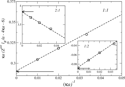
Figure 2: Asymptotic expansion plots for charged spheres in a 1:1 salt (main graph), together with asymmetric 1:2 and 2:1 salts (insets). The main graph shows $\kappa a(Z_{\rm eff}^{\rm sat}l_{B}/a-4\kappa a-6)$ as a function of $1/(\kappa a)$. The dashed linear curve is for the line that passes through the two points associated to the largest values of $\kappa a$ (50 and 100). The arrow is the predicted asymptotic limit $\pi^{2}/3-3$. The symbols correspond to the saturated effective charge obtained from the numerical solution of Eq. (3.1) with $\alpha=2$. The 2:1 inset shows the counterpart, $\kappa a(Z_{\rm eff}^{\rm sat}l_{B}/a-6\kappa a-7)$ where the limit is predicted to be $\simeq 3.844$. The 1:2 inset is constructed similarly from Eq. (6.21), for which the arrow indicating the intercept is at -0.089.

In the saturation limit $\lambda\to\infty$, the requirement $f_{\rm sat}(\kappa a)=1$ implies the iteratively generated large-$\kappa a$ expansion

$$t_{\rm sat}(\kappa a)=1+\frac{1}{2}\frac{1}{\kappa a}-\left(\frac{5}{4}-\frac{\pi^{2}}{12}\right)\frac{1}{(\kappa a)^{2}}+\cdots.$$ (4.27)

Here, we used that $g_{2}(1)$ is given by (4.26). We cannot go beyond the indicated order because the next term needs the iteration with the diverging value of $g_{2}(1+1/(2\kappa a))$. This indicates that the next-order singular term has a form different from $1/(\kappa a)^{3}$.

Using the prescription (3.28), the corresponding saturation value of the effective charge exhibits the large-$\kappa a$ expansion of the form

$$Z_{\rm eff}^{\rm sat}\frac{l_{\rm B}}{a}=4\kappa a+6+\left(\frac{\pi^{2}}{3}-3\right)\frac{1}{\kappa a}+o\left(\frac{1}{\kappa a}\right).$$ (4.28)

The numerical check of the prefactor to the third $1/(\kappa a)$ term is presented in Fig. 2. Indirectly, the plot also assesses the correctness of the dominant terms $4\kappa a+6$.

V 2:1 electrolyte

For the asymmetric $2:1$ electrolyte in contact with the cylindrical $\alpha=1$ or spherical $\alpha=2$ colloids, the PB equation in the reduced distance $x=\kappa r$ takes the form

$$\phi^{\prime\prime}(x)+\frac{\alpha}{x}\phi^{\prime}(x)=\frac{1}{3}\left[{\rm e}^{\phi(x)}-{\rm e}^{-2\phi(x)}\right].$$ (5.1)

Being motivated by the exact planar solution (2.43), we search the electrostatic potential in an ansatz form

$$\phi(x)=\ln\left\{1+\frac{6f(x)}{\left[1-f(x)\right]^{2}}\right\}.$$ (5.2)

Introducing

$$t(x)=\frac{A(\lambda)}{6}\frac{{\rm e}^{-x}}{x^{\alpha/2}},$$ (5.3)

$f(x)\sim t(x)$ is the leading large-distance form. Inserting the ansatz (5.2) into the PB equation (5.1), we obtain the differential equation for the $f$-function:

$$\left[f^{\prime\prime}(x)+\frac{\alpha}{x}f^{\prime}(x)-f(x)\right]\left[1-f^{2}(x)\right]\left[f^{2}(x)+4f(x)+1\right]$$

$$-2\left[f^{3}(x)+3f^{2}(x)+3f(x)-1\right]\left[f(x)+f^{\prime}(x)\right]\left[f(x)-f^{\prime}(x)\right] = 0.$$ (5.4)

We again expect that the $f$-function is expressible as a series

$$f(x)=tg(x),\qquad g(x)=1+\sum_{k=1}^{\infty}\frac{1}{x^{k}}g_{k}(t).$$ (5.5)

The $g$-function satisfies the differential equation

$$\left[g^{\prime\prime}(x)-2g^{\prime}(x)+\frac{\alpha(2-\alpha)}{4x^{2}}g(x)\right]\left[1-t^{2}g^{2}(x)\right]\left[t^{2}g^{2}(x)+4tg(x)+1\right]$$

$$-2t\left[t^{3}g^{3}(x)+3t^{2}g^{2}(x)+3tg(x)-1\right]\left[g^{\prime}(x)-\frac{\alpha}{2x}g(x)\right]\left[\left(2+\frac{\alpha}{2x}\right)g(x)-g^{\prime}(x)\right] = 0.$$ (5.6)

V.1 Cylindrical geometry

For the cylindrical $\alpha=1$ geometry, setting to zero the coefficient to $1/x$ in (5.6), $g_{1}(t)$ obeys the differential equation

$$t(1+4t-4t^{3}-t^{4})g_{1}^{\prime\prime}(t)$$

$$+(3+8t+12t^{2}+t^{4})g_{1}^{\prime}(t)$$

$$+2(-1+3t+3t^{2}+t^{3}) = 0.$$ (5.7)

The solution of this equation with the BC $g_{1}(0)=-1/8$, regular as $t\to 0$, is found to be

$$g_{1}(t)=\frac{29}{24}-\frac{2}{3}t-\frac{1}{12}t^{2}-\frac{4}{3}\frac{1}{1+t}.$$ (5.8)

Similarly, we obtain

$$g_{2}(t) = -\frac{2543}{2^{7}\times 3^{2}}+\frac{11}{2\times 3^{2}}t+\frac{5}{2^{5}}t^{2}+\frac{1}{3^{2}}t^{3}+\frac{1}{2^{4}\times 3^{2}}t^{4}$$

$$+\frac{2\times 5}{3}\frac{1}{1+t}-\frac{5\times 7}{2\times 3^{2}}\frac{1}{(1+t)^{2}}+\frac{2^{3}}{3^{2}}\frac{1}{(1+t)^{3}},$$

$$g_{3}(t) = \frac{5\times 41\times 659}{2^{10}\times 3^{3}}+\frac{7^{2}}{2^{4}\times 3^{2}}t-\frac{617}{2^{9}\times 3}t^{2}-\frac{17}{2^{2}\times 3^{3}}t^{3}$$

$$-\frac{13\times 19}{2^{7}\times 3^{3}}t^{4}-\frac{1}{2^{3}\times 3^{2}}t^{5}-\frac{1}{2^{6}\times 3^{3}}t^{6}$$

$$-\frac{193}{2\times 3^{2}}\frac{1}{1+t}+\frac{11173}{2^{5}\times 3^{3}}\frac{1}{(1+t)^{2}}$$

$$-\frac{4649}{2^{4}\times 3^{3}}\frac{1}{(1+t)^{3}}+\frac{43}{3^{2}}\frac{1}{(1+t)^{4}}-\frac{2^{5}}{3^{3}}\frac{1}{(1+t)^{5}},$$

etc. In general, $g_{k}(t)$ $(k=1,2,\ldots)$ is the sum of two finite polynomial, one of the $2k$th order in $t$ and the other of the $(2k-1)$th order in $1/(1+t)$.

In the saturation limit $\lambda\to\infty$, the requirement $f_{\rm sat}(\kappa a)=1$ implies the iteratively generated large-$\kappa a$ expansion

$$t_{\rm sat}(\kappa a) = 1+\frac{5}{2^{3}\times 3}\frac{1}{\kappa a}+\frac{5\times 41}{2^{7}\times 3^{2}}\frac{1}{(\kappa a)^{2}}$$ (5.11)

$$-\frac{12583}{2^{10}\times 3^{2}}\frac{1}{(\kappa a)^{3}}+\cdots\equiv\frac{A_{\rm sat}}{6}\frac{{\rm e}^{-\kappa a}}{\sqrt{\kappa a}}.\phantom{aaa}$$

Using the prescription (3.19), for large values of $\kappa a$ the saturation value of the effective charge behaves as

$$\lambda_{\rm eff}^{\rm sat}l_{\rm B}=3\kappa a+\frac{7}{4}+\frac{5}{12}\frac{1}{\kappa a}-\frac{703}{192}\frac{1}{(\kappa a)^{2}}+O\left(\frac{1}{(\kappa a)^{3}}\right).$$ (5.12)

The first two terms of this series have been obtained in Ref. Tellez04 . The numerical checks of the coefficients to the $1/(\kappa a)$ and $1/(\kappa a)^{2}$ terms are presented in the main graph of Fig. 3.

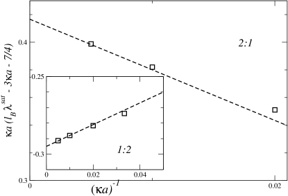
Figure 3: Asymptotic expansion plots for cylinders in 2:1 and 1:2 salts. The main graph for the 2:1 case shows $\kappa a(\lambda_{\rm eff}^{\rm sat}l_{B}-3\kappa a-7/4)$ versus $1/(\kappa a)$. The linear dashed curve displays the prediction embodied in Eq. (5.12), $5/12-703(\kappa a)^{-1}/192$. The inset displays expression (6.13) as a function of $1/(\kappa a)$. The dashed linear curve is for the prediction of Eq. (6.12), $-0.295+0.700/(\kappa a)$. As in previous figures, the symbols show the data obtained from solving numerically the Poisson-Boltzmann equation.

V.2 Spherical geometry

For the spherical $\alpha=2$ geometry, setting to zero the coefficient to $1/x$ in (5.6), $g_{1}(t)$ fulfills the equation

$$t(1+4t-4t^{3}-t^{4})g_{1}^{\prime\prime}(t)$$

$$+(3+8t+12t^{2}+t^{4})g_{1}^{\prime}(t)$$

$$+4(-1+3t+3t^{2}+t^{3}) = 0.$$ (5.13)

Considering the BC $g_{1}(0)=0$, the solution is

$$g_{1}(t)=\frac{8}{3}-\frac{4}{3}t-\frac{1}{6}t^{2}-\frac{8}{3}\frac{1}{1+t}.$$ (5.14)

Setting to zero the coefficient to $1/x^{2}$ in (5.6), we obtain the differential equation for $g_{2}(t)$ of the form

$$P(t)g_{2}^{\prime\prime}(t)+Q(t)g_{2}^{\prime}(t)+R(t)=0,$$ (5.15)

where

$$P(t) = 9t(1+t)^{5}(1+3t-3t^{2}-t^{3}),$$ (5.16)

$$Q(t) = 9(1+t)^{4}(3+8t+12t^{2}+t^{4}),$$ (5.17)

$$R(t) = 78+51t+84t^{2}+252t^{3}-1912t^{4}$$ (5.18)

$$-2560t^{5}-1860t^{6}-430t^{7}+314t^{8}$$

$$+189t^{9}+32t^{10}+2t^{11}.$$

The function $g_{2}(t)$ is an infinite polynomial in $t$ which diverges for all $t>1$. The value of $g_{2}$ at $t=1$ is of our primary interest. Denoting $g_{2}(1)\equiv{\cal A}$, by using Mathematica it can be shown that

$${\cal A} = -\frac{4}{9}-\frac{\pi^{2}}{6}-\frac{2}{\sqrt{3}}\ln(2-\sqrt{3})+\frac{1}{3}[\ln(2-\sqrt{3})]^{2}$$ (5.19)

$$-\frac{1}{6}\left[\ln(3+\sqrt{3})\right]^{2}-\frac{1}{3}\ln(2-\sqrt{3})\ln(3-\sqrt{3})$$

$$-\frac{1}{3}{\rm Li}_{2}\left(\frac{1}{6}(3-\sqrt{3})\right)-\frac{1}{3}{\rm Li}_{2}(-2+\sqrt{3})$$

$$\simeq -0.27962,$$

where ${\rm Li}_{2}(z)$ is the polylogarithm function defined by

$${\rm Li}_{2}(z)=\sum_{k=1}^{\infty}\frac{z^{k}}{k^{2}},\qquad|z|\leq 1.$$ (5.20)

The saturation condition $f_{\rm sat}(\kappa a)=1$ implies the large-$\kappa a$ expansion

$$t_{\rm sat}(\kappa a) = 1+\frac{1}{6}\frac{1}{\kappa a}+\left(\frac{7}{36}-{\cal A}\right)\frac{1}{(\kappa a)^{2}}\cdots$$ (5.21)

$$\equiv \frac{A_{\rm sat}}{6}\frac{{\rm e}^{-\kappa a}}{\kappa a}.$$

With respect to the prescription (3.28), the saturation value of the effective charge behaves for large values of $\kappa a$ as follows

$$Z_{\rm eff}^{\rm sat}\frac{l_{\rm B}}{a} = 6\kappa a+7+\left(\frac{13}{6}-6{\cal A}\right)\frac{1}{\kappa a}+o\left(\frac{1}{\kappa a}\right)$$ (5.22)

$$\simeq 6\kappa a+7+3.844\frac{1}{\kappa a}+o\left(\frac{1}{\kappa a}\right).$$

The first two terms of this expansion are in full agreement with the result of Ref. Tellez04 . The prefactor to the $1/(\kappa a)$ term is checked against the numerical resolution in Fig. 2.

VI 1:2 electrolyte

For the asymmetric $1:2$ electrolyte, the PB equation takes the form

$$\phi^{\prime\prime}(x)+\frac{\alpha}{x}\phi^{\prime}(x)=\frac{1}{3}\left[{\rm e}^{2\phi(x)}-{\rm e}^{-\phi(x)}\right].$$ (6.1)

With regard to the exact planar solution (2.47), the electrostatic potential is searched in an ansatz form

$$\phi(x)=-\ln\left\{1-\frac{6f(x)}{\left[1+f(x)\right]^{2}}\right\}.$$ (6.2)

Introducing

$$t(x)=\frac{A(\lambda)}{6}\frac{{\rm e}^{-x}}{x^{\alpha/2}},$$ (6.3)

$f(x)\sim t(x)$ in the leading large-distance order.

Inserting (6.2) into the PB equation (6.1), the $f$-function obeys the differential equation

$$\left[f^{\prime\prime}(x)+\frac{\alpha}{x}f^{\prime}(x)-f(x)\right]\left[1-f^{2}(x)\right]\left[f^{2}(x)-4f(x)+1\right]$$

$$-2\left[f^{3}(x)-3f^{2}(x)+3f(x)+1\right]\left[f(x)+f^{\prime}(x)\right]\left[f(x)-f^{\prime}(x)\right] = 0.$$ (6.4)

Writing the $f$-function as a series

$$f(x)=tg(x),\qquad g(x)=1+\sum_{k=1}^{\infty}\frac{1}{x^{k}}g_{k}(t),$$ (6.5)

the $g$-function satisfies the differential equation

$$\left[g^{\prime\prime}(x)-2g^{\prime}(x)+\frac{\alpha(2-\alpha)}{4x^{2}}g(x)\right]\left[1-t^{2}g^{2}(x)\right]\left[t^{2}g^{2}(x)-4tg(x)+1\right]$$

$$-2t\left[t^{3}g^{3}(x)-3t^{2}g^{2}(x)+3tg(x)+1\right]\left[g^{\prime}(x)-\frac{\alpha}{2x}g(x)\right]\left[\left(2+\frac{\alpha}{2x}\right)g(x)-g^{\prime}(x)\right] = 0.$$ (6.6)

VI.1 Cylindrical geometry

For $\alpha=1$, setting to zero the coefficient to $1/x$ in (6.6), $g_{1}(t)$ must obey the equation

$$t(1-4t+4t^{3}-t^{4})g_{1}^{\prime\prime}(t)$$

$$+(3-8t+12t^{2}+t^{4})g_{1}^{\prime}(t)$$

$$+2(1+3t-3t^{2}+t^{3}) = 0.$$

The regular solution of this equation with the BC $g_{1}(0)=-1/8$ reads

$$g_{1}(t)=\frac{29}{24}+\frac{2}{3}t-\frac{1}{12}t^{2}-\frac{4}{3}\frac{1}{1-t}.$$ (6.8)

In the same way, we get

$$g_{2}(t) = -\frac{2543}{2^{7}\times 3^{2}}-\frac{11}{2\times 3^{2}}t+\frac{5}{2^{5}}t^{2}-\frac{1}{3^{2}}t^{3}+\frac{1}{2^{4}\times 3^{2}}t^{4}$$

$$+\frac{2\times 5}{3}\frac{1}{1-t}-\frac{5\times 7}{2\times 3^{2}}\frac{1}{(1-t)^{2}}+\frac{2^{3}}{3^{2}}\frac{1}{(1-t)^{3}},$$

$$g_{3}(t) = \frac{5\times 41\times 659}{2^{10}\times 3^{3}}-\frac{7^{2}}{2^{4}\times 3^{2}}t-\frac{617}{2^{9}\times 3}t^{2}+\frac{17}{2^{2}\times 3^{3}}t^{3}$$

$$-\frac{13\times 19}{2^{7}\times 3^{3}}t^{4}+\frac{1}{2^{3}\times 3^{2}}t^{5}-\frac{1}{2^{6}\times 3^{3}}t^{6}$$

$$-\frac{193}{2\times 3^{2}}\frac{1}{1-t}+\frac{11173}{2^{5}\times 3^{3}}\frac{1}{(1-t)^{2}}$$

$$-\frac{4649}{2^{4}\times 3^{3}}\frac{1}{(1-t)^{3}}+\frac{43}{3^{2}}\frac{1}{(1-t)^{4}}-\frac{2^{5}}{3^{3}}\frac{1}{(1-t)^{5}},$$

etc.

In the saturation limit $\lambda\to\infty$, the requirement $f_{\rm sat}(\kappa a)=2-\sqrt{3}$ implies the large-$\kappa a$ expansion

$$t_{\rm sat}(\kappa a) = 2-\sqrt{3}+\left(-\frac{67}{12}+\frac{79}{8\sqrt{3}}\right)\frac{1}{\kappa a}$$ (6.11)

$$+\left(\frac{17053}{576}-\frac{19765}{384\sqrt{3}}\right)\frac{1}{(\kappa a)^{2}}$$

$$+\left(-\frac{751423}{4608}+\frac{869059}{3072\sqrt{3}}\right)\frac{1}{(\kappa a)^{3}}+\cdots$$

$$\equiv \frac{A_{\rm sat}}{6}\frac{{\rm e}^{-\kappa a}}{\sqrt{\kappa a}}.\phantom{aaa}$$

With the aid of (3.19), for large values of $\kappa a$ the saturation value of the effective charge behaves as

$$\lambda_{\rm eff}^{\rm sat}l_{\rm B} = 3(2-\sqrt{3})\kappa a+\left(-\frac{29}{2}+\frac{35\sqrt{3}}{4}\right)$$ (6.12)

$$+\left(\frac{491}{6}-\frac{569}{4\sqrt{3}}\right)\frac{1}{\kappa a}$$

$$+\left(-\frac{43519}{96}+\frac{50329}{64\sqrt{3}}\right)\frac{1}{(\kappa a)^{2}}+O\left(\frac{1}{(\kappa a)^{3}}\right)$$

$$\simeq 0.804\,\kappa a+0.655-\frac{0.295}{\kappa a}$$

$$+\frac{0.700}{(\kappa a)^{2}}+O\left(\frac{1}{(\kappa a)^{3}}\right).$$

The first two terms of this series have been obtained in Ref. Tellez04 . The numerical checks of the coefficients to the $1/(\kappa a)$ and $1/(\kappa a)^{2}$ terms are presented in Fig. 3. The quantity plotted in the inset is thus

$$\kappa a\left[\lambda_{\rm eff}^{\rm sat}l_{\rm B}-3(2-\sqrt{3})\kappa a+\left(\frac{29}{2}-\frac{35\sqrt{3}}{4}\right)\right].$$ (6.13)

VI.2 Spherical geometry

For $\alpha=2$, setting to zero the coefficient to $1/x$ in (6.6), $g_{1}(t)$ obeys the equation

$$t(1-4t+4t^{3}-t^{4})g_{1}^{\prime\prime}(t)$$

$$+(3-8t+12t^{2}+t^{4})g_{1}^{\prime}(t)$$

$$+4(1+3t-3t^{2}+t^{3}) = 0.$$ (6.14)

The regular solution of this equation with the BC $g_{1}(0)=0$ reads

$$g_{1}(t)=\frac{8}{3}+\frac{4}{3}t-\frac{1}{6}t^{2}-\frac{8}{3}\frac{1}{1-t}.$$ (6.15)

Setting to zero the coefficient to $1/x^{2}$ in (6.6), we obtain the differential equation for $g_{2}(t)$ of type (5.15) with the polynomial coefficients

$$P(t) = 9t(1-t)^{5}(1-3t-3t^{2}-t^{3}),$$ (6.16)

$$Q(t) = 9(1-t)^{4}(3-8t+12t^{2}+t^{4}),$$ (6.17)

$$R(t) = -78+51t-84t^{2}+252t^{3}+1912t^{4}$$ (6.18)

$$-2560t^{5}+1860t^{6}-430t^{7}-314t^{8}$$

$$+189t^{9}-32t^{10}+2t^{11}.$$

For our purpose, the value of $g_{2}$ at $t=2-\sqrt{3}$ will be important. Denoting $g_{2}(2-\sqrt{3})\equiv{\cal B}$, using Mathematica we got

$${\cal B} = -\frac{130}{9}+10\sqrt{3}-\frac{\pi^{2}}{9}-\frac{4}{\sqrt{3}}\ln 2-2\sqrt{3}\ln 3$$ (6.19)

$$+\frac{1}{3}\left[\ln 12-\frac{7}{\sqrt{3}}\right]\ln(2-\sqrt{3})+\frac{2}{3}[\ln(2-\sqrt{3})]^{2}$$

$$-\frac{29}{3\sqrt{3}}\ln(\sqrt{3}-1)+\frac{5}{3\sqrt{3}}\ln(\sqrt{3}+1)$$

$$-\frac{4}{3}{\rm Li}_{2}(-2+\sqrt{3})+\frac{1}{3}{\rm Li}_{2}(-6+4\sqrt{3})$$

$$\simeq 1.71475.$$

In the saturation regime, the condition $f_{\rm sat}(\kappa a)=2-\sqrt{3}$ implies the large-$\kappa a$ expansion

$$t_{\rm sat}(\kappa a) = (2-\sqrt{3})+\left(-\frac{35}{3}+\frac{41}{2\sqrt{3}}\right)\frac{1}{\kappa a}$$ (6.20)

$$+\left[\frac{1123}{18}-\frac{1291}{12\sqrt{3}}-(2-\sqrt{3}){\cal B}\right]\frac{1}{(\kappa a)^{2}}$$

$$+\cdots\equiv\frac{A_{\rm sat}}{6}\frac{{\rm e}^{-\kappa a}}{\kappa a}.$$

Based on (3.28), the large-$\kappa a$ expansion of the saturation value of the effective charge is obtained in the form

$$Z_{\rm eff}^{\rm sat}\frac{l_{\rm B}}{a} = 6(2-\sqrt{3})\kappa a+\left(-58+35\sqrt{3}\right)$$ (6.21)

$$+\left[\frac{913}{3}-\frac{1045}{2\sqrt{3}}-6(2-\sqrt{3}){\cal B}\right]\frac{1}{\kappa a}+o\left(\frac{1}{\kappa a}\right)$$

$$\simeq 1.608\kappa a+2.622-0.089\frac{1}{\kappa a}+o\left(\frac{1}{\kappa a}\right).$$

The first two terms of the expansion coincide with those obtained in Ref. Tellez04 . The prefactor to the third $1/(\kappa a)$ term is checked against numerics in Fig. 2.

VII Conclusion

In this work, we have revisited the analytical results following from a multiple scale expansion of the non-linear Poisson-Boltzmann equation, for both cylindrical and spherical macro-ions. The corresponding planar case is analytically solvable. Three types of electrolyte have been addressed: symmetric ones where the co-and counter-ions bear the same charge in absolute value (1:1 case), as well as asymmetric 1:2 and 2:1 situations. The latter two cases are not equivalent due to the non-linear nature of the differential equation to be solved, although they can yield the same Debye length. Inspecting the structure of the double series appearing intimates that a partial resummation can be performed. In doing so, and restricting to the 1:1 case for the sake of simplicity, the dimensionless electrostatic potential $\phi$ appears to depend on radial distance $r$ through

$$\phi(r)\,=\,2\,\ln\left(\frac{1+f(x)}{1-f(x)}\right)$$ (7.1)

where $x=\kappa r$, and

$$f(x)\,=\,t\left[1+\sum_{k=1}^{\infty}\frac{g_{k}(t)}{x^{k}}\right]\quad;\quad t\,=\,\frac{A}{4}\frac{{\rm e}^{-x}}{x^{\alpha/2}}.$$ (7.2)

Here, $\alpha$ is a fingerprint of geometry (more precisely, of curvature, with $\alpha=0$ for plates, $\alpha=1$ for cylinders, $\alpha=2$ for spheres) and $A$ parameterizes the solution: different values of $A$ correspond to different bare charges. The saturation phenomenon means that while $A$ changes in some finite interval $[0,A_{\text{sat}}]$, the bare charge varies between 0 and $\infty$. More precisely, since one has $\phi\sim t$ for $r\to\infty$, $A$ is directly related to the effective charge of the macro-ion. For 1:2 and 2:1 electrolytes, relation (7.1) changes to some extent (see Eqs. (5.2) and (6.2)), while the relation between $f$, $t$ and $A$ in Eq. (7.2) is essentially unaffected.

The planar case is such that $\kappa a\to\infty$, with $f(x)=t=A\,e^{-x}/4$. As a consequence, our family of solutions is of “quasi-planar” type, which is of course quite expected in the limit where the macro-ion radius $a$ is much larger than the Debye length $1/\kappa$. Yet, the details of this quasi-planarity are non trivial, and are such that particularly convenient expansion properties ensue in the asymptotic limit $\kappa a\to\infty$. As an illustration, we have computed saturated effective charges (meaning in the limit where the macro-ion bare charge becomes very large) where our scheme yields an exact expansion in inverse powers of $\kappa a$. Indeed, a careful numerical calculation of the same quantities from solving directly the Poisson-Boltzmann equation, allows to check, term by term, the predicted expansion. This requires an extrapolation procedure, which has been presented, for extracting the saturation values from results that are necessarily obtained at finite although large bare charges.

So far, not enough is known on the planar case for different asymmetries than 1:2 and 2:1, so that our approach cannot be generalized to such situations. What misses is the explicit structure of the counterpart of Eqs. (7.1), (5.2) and (6.2) in these cases Tellez11 .

- (1) P. Debye and E. Hückel, Phys. Zeitschr. 24, 185 (1923).
- (2) G. L. Gouy, J. Phys. 9, 457 (1910).
- (3) D. L. Chapman, Philos. Mag. 25, 475 (1913).
- (4) E. J. W. Verwey and J. Th. G. Overbeek, Theory of the Stability of Lyophobic Colloids (Elsevier, New York, 1948.
- (5) L. Belloni, Colloids Surf. A 140, 227 (1998).
- (6) J. P. Hansen and H. Löwen, Ann. Rev. Phys. Chem. 51, 209 (2000).
- (7) D. B. Lukatsky and S. A. Safran, Phys. Rev. E 63, 011405 (2001).
- (8) Y. Levin, Rep. Prog. Phys. 65, 1577 (2002).
- (9) S. Alexander, P. M. Chaikin, P. Grant, G. J. Morales and P. Pincus, J. Chem. Phys. 80, 5776 (1984).
- (10) A. Diehl, M. C. Barbosa and Y. Levin, Europhys. Lett. 53, 86 (2001).
- (11) E. Trizac, L. Bocquet and M. Aubouy, Phys. Rev. Lett. (2002).
- (12) L. Bocquet, E. Trizac and M. Aubouy, J. Chem. Phys. 117, 8138 (2002).
- (13) G. Téllez and E. Trizac, Phys. Rev. E 70, 011404 (2004).
- (14) L. Šamaj and I. Travěnec, J. Stat. Phys. 101, 713 (2000).
- (15) L. Šamaj and Z. Bajnok, Phys. Rev. E 72, 061503 (2005).
- (16) L. Šamaj, J. Stat. Phys. 120, 125 (2005).
- (17) G. Téllez, J. Stat. Mech., P10001 (2005).
- (18) L. Šamaj, J. Stat. Phys. 124, 1179 (2006).
- (19) R. D. Groot, J. Chem. Phys. 95, 9191 (1991).
- (20) A. Diehl and Y. Levin, J. Chem. Phys. 121, 12100 (2004).
- (21) G. Téllez, Phil. Trans. R. Soc. A 369, 322 (2011).
- (22) G. V. Ramanathan, J. Chem. Phys. 78, 3223 (1983).
- (23) G. V. Ramanathan, J. Chem. Phys. 88, 3887 (1988).
- (24) E. Trizac and G. Téllez, Phys. Rev. Lett. 96, 038302 (2006).
- (25) I. A. Shkel, O. V. Tsodikov, and M. T. Record, J. Phys. Chem. B 104, 5161 (2000).
- (26) M. Aubouy, E. Trizac, and L. Bocquet, J. Phys. A: Math. Gen. 36, 5835 (2003).
- (27) The mean-field treatment adopted does not discriminate the potential created by a disk in 2D from that of an infinite cylinder in 3D. The treatment exhibits in this sense some geometrical degeneracy.
- (28) The validity of the mean-field view deteriorates when the valency of counter-ions increases, see e.g. Levin02 .
- (29) It can be checked from the expressions given in Aubouy03 –and again considering only the dominant plus first sub-dominant contributions– that beyond the saturation limit, a similar remark holds for the full functional dependence of effective charges as a function of bare charges, when expressed in terms of colloid curvature. Of course, this feature is not restricted to 1:1 electrolytes.