A complete set of eigenstates for position-dependent massive particles in a Morse-like scenario

Abstract

In this work we analyze a system consisting in two-dimensional position-dependent massive particles in the presence of a Morse-like potential in two spatial dimensions. We obtain the exact wavefunctions and energies for a complete set of eigenstates for a given dependence of the mass with the spatial variables. Furthermore, we argue that this scenario can be play an important role to construct more realistic ones by using their solution in perturbative approaches.

I Introduction

Some years ago, the materials science took an important step forward by obtaining the fabrication of small conducting devices known as quantum dots (QDs) Alhassid . In those devices, it is possible to confine several thousand electrons in a small region whose linear size is about $0.1-1\mu m$ rmp1 . The fundamental characteristic of QDs is that they are typically formed by a two-dimensional electron gas, where, by applying an electrostatic potential, the electrons are confined to a small region, which is called “dot”, in the interface region of a semiconductor. A very important advantage of QDs is that their transport properties are readily measured, allowing an experimental control. Moreover, the effects of time-reversal symmetry breaking can be easily measured by applying a magnetic field prl0 . Nowadays, a variety of theoretical and experimental research about small conducting devices, such as QDs, has been the focus of many scientists and engineers attention prb1 ; prb2 ; pre1 ; prl1 . From a phenomenological viewpoint, QDs are very small structures, where the laws of quantum mechanics (QM) are the most important ingredients to describe their properties. Thus, as a natural consequence of practical applicability of the theoretical framework of QM, a great interest arises for exact solutions of two-dimensional confined systems, which can be fundamental to explore the physics in small conducting devices, such as the QDs. In the light of these facts, it was shown in Ref. Lozada-Dong-Yu that it is possible to find exact solutions of the two-dimensional Schrödinger equation with the position-dependent mass (PDM) for the square well potential in the semiconductor quantum dots (SQDs) system. Another important work in this context, it was presented by Schmidt, Azeredo, and Gusso Schmidt-Azeredo-Gusso , where the authors have studied both the problems of quantum wave packet revivals on two-dimensional infinite circular quantum wells (CQWs) and circular quantum dots (CQDs) with PDM, showing the results for the eigenfunctions, eigenenergies and the revival time for spatially localized electronic Gaussian wave packets. At this point, it is important to highlight that the importance in adding a PDM is due to the fact that the system will take into account the spatial variation of the semiconductor BenDaniel-Duke ; Gora-Williams ; Bastard ; Ross ; Zhu-Kroemer ; Li-Kuhn ; Cavalcante-Filho-Almeida-Freire ; Dutra-Oliveira . However, as consequence of inclusion a PDM, the system becomes ambiguous at the quantum level, and the ordering ambiguity problem (OAP) is one of the long standing unsolved questions in quantum mechanics. As we know the OAP has attracted the attention of some of the founders of the quantum mechanics, namely, Born, Jordan, Weyl, Dirac and von Newmann worked on this problem, as can be verified from the review by Shewell Shewell . This is viewed as a deep problem in QM, which has advanced very few along the last decades. But all is not lost, it was shown that the ordering ambiguous problem has a very special importance for the modeling of some experimental situations like electrons in perturbed periodic lattices Slater , impurities states and cyclotron resonance in semiconductors Luttinger , the structure of electronic excitation levels in insulating crystals Wannier , the dependence of nuclear forces on the relative velocity of the two nucleons rojo ; razavy , and more recently the study of semiconductor heterostructures Bastard ; weisbuch ; ref1 ; ref2 ; ref3 . Moreover, some time ago, it was discussed in the literature the exact solvability of some classes of one-dimensional Hamiltonians, where the potentials has a PDM, with ordering ambiguity pla2000 , after that, a large number of works regarding one-dimensional Hamiltonians with ordering ambiguity has emerged in the scientific community along the last few years m1 ; m2 ; m3 ; m4 ; m5 ; m6 ; jpa2006 . Another interesting research line regards to the supersymmetry approach to one-dimensional quantum systems with spatially-dependent mass, by including their ordering ambiguities dependence dutra2 ; schimidt1 ; quesne ; sever ; halberg ; carinena ; ganguly ; roy ; mustafa ; tanaka ; koca ; znojil ; cg1 ; Cg2 ; a0 ; a1 ; a3 ; a4 ; a5 ; a6 ; a7 ; a8 ; a9 ; npb ; epl05 . On the other hand, as far as we know, some physical systems like ones where a magnetic field is present pla87 ; pra89 ; pla91 ; abdalla2007 , lead naturally to the necessity of a two-dimensional analysis. In the face of this situation, it was presented in Ref.dutra-juliano a general approach for the problem of a particle with PDM interacting with a two-dimensional potential well with finite depth, where the ordering ambiguity was taken in account. In that work, it was shown that the considered system retain an infinite set of quantum states, which usually do not happens in the case of the constant mass systems. Furthermore, it was verified also that the SU(2) coherent state corresponds to a stationary state. Also recently, numerous other theoretical studies have been conducted on two-dimensional position-dependent mass Schrödinger equation (PDMSE). These include the two-dimensional quantum rotor with two effective masses cc1 , kinetic operator in cylindrical coordinates cc2 , exact solutions for the PDMSE in an annular billiard with impenetrable walls cc3 , and a particle with spin 1/2 moving in a plane cc4 .

Here, we will address the position-dependent mass (PDM) type of the systems in two spatial dimensions (2D) by using Cartesian coordinates. We will introduce a very interesting system where, as we are going to see below in the manuscript, the relation between the quantum numbers introduced along the procedure of resolving the equations of the system and the energy eigenstates organization is somewhat remarkable.

This paper is organized as follows. In Section redII, we review the effective Schrödinger equation in two-dimensional Cartesian coordinates. In Section redIII, we introduce the Position-dependent massive particle with Morse-like terms and its exact solutions. In Section redIV, we present our conclusions and directions for future work.

II Effective Schroedinger equation in two-dimensional Cartesian coordinates: A brief review

In this section, we will recapitulate the results presented some years ago in Ref. Dutra-Oliveira . Let us start with the ordering defined by von Roos Ross ; pla2000 for the Hamiltonian operator, which in one-dimensional space is written in the following form

$$\hat{H}=\frac{1}{4}\left(M^{\alpha}\hat{p}M^{\beta}\hat{p}M^{\gamma}+M^{\gamma}\hat{p}M^{\beta}\hat{p}M^{\alpha}\right)+V(x),$$ (1)

where $\hat{p}$ is the momentum operator and $M=M(x)$ is the position-dependent effective mass. Moreover, $\alpha,\beta$ and $\gamma$ are arbitrary ordering parameters which must to obey the relation

$$\alpha+\beta+\gamma=-1.$$ (2)

At this point, it is important to highlight that the above relation is necessary to get the correct classical limit.

Applying the canonical commutation relations, we have

$$M^{\gamma}\hat{p}M^{\beta}\hat{p}M^{\alpha}=\frac{\hat{p}^{2}}{M}-i\hbar(\beta+2\alpha)\frac{M^{\prime}}{M^{2}}\hat{p}-\hbar^{2}\alpha(\beta+\alpha-1)\frac{(M^{\prime})^{2}}{M^{3}}-\hbar^{2}\alpha\frac{M^{\prime\prime}}{M^{2}}.$$ (3)

Through the relation (2), the effective Hamiltonian operator pla2000 is given by

$$H=\frac{1}{2\,M}\hat{p}^{2}+\frac{i\,\hbar}{2}\frac{M^{\prime}}{M^{2}}\hat{p}+U(\alpha,\gamma,x)+V(x),$$ (4)

where the effective potential $U(\alpha,\gamma,x)$ is written as

$$U(\alpha,\gamma,x)=-\frac{\hbar^{2}}{4M^{3}}\left[(\alpha+\gamma)M\left(\frac{\partial^{2}M}{\partial x^{2}}\right)-2(\alpha+\gamma+\alpha\gamma)\left(\frac{\partial M}{\partial x}\right)^{2}\right].$$ (5)

Therefore, we can now write the effective Schroedinger equation in the form

$$-\frac{\hbar^{2}}{2\,M(x)}\frac{d^{2}\psi}{dx^{2}}+\frac{\hbar^{2}}{2}\left[\frac{dM/dx}{M^{2}}\right]\frac{d\psi}{dx}+[V(x)+U(\alpha,\gamma,x)-E]\psi=0.$$ (6)

In the case of a set of two-dimensional Cartesian coordinates, where $M=M(x,y)$, the effective Hamiltonian operator

$$H=\frac{1}{2\,M(x,y)}(\hat{p_{x}}^{2}+\hat{p_{y}}^{2})+\frac{i\,\hbar}{2}\left(\frac{\frac{\partial M}{\partial x}\hat{p_{x}}+\frac{\partial M}{\partial y}\hat{p_{y}}}{M^{2}}\right)+U(\alpha.\gamma,x)+V(x,y),$$ (7)

where $U(\alpha,\gamma,x,y)$ is the effective potential. Now it can be written in the form Dutra-Oliveira

$$U(\alpha,\gamma,x,y)=-\frac{\hbar^{2}}{4M}\left\{(\alpha+\gamma)\,\frac{M_{xx}+M_{yy}}{M}-2(\alpha+\gamma+\alpha\gamma)\left[\left(\frac{M_{x}}{M}\right)^{2}+\left(\frac{M_{y}}{M}\right)^{2}\right]\right\},$$ (8)

with $M_{x}\equiv\partial M/\partial x$ and $M_{y}\equiv\partial M/\partial y$. Therefore, we have

$$H=\frac{1}{2\,M}\overrightarrow{p}^{2}+\frac{i\hbar}{2}\,\frac{1}{M^{2}}\,\overrightarrow{\nabla}M.\overrightarrow{p}+U(\alpha,\gamma,x,y)+V(x,y),$$ (9)

where, in this case

$$U(\alpha,\gamma,x,y)\equiv-\frac{\hbar^{2}}{4\,M}\left[(\alpha+\gamma)\,\frac{{\nabla}^{2}M}{M}-2(\alpha+\gamma+\alpha\gamma)\left(\frac{\overrightarrow{\nabla}M}{M}\right)^{2}\right].$$ (10)

In the next step we can use a typical Schroedinger equation

$$-\frac{\hbar^{2}}{2\,M(x,y)}\,\nabla^{2}\,\chi+V_{eff}(x,y)\,\chi=E\,\chi,$$ (11)

and if $\chi(x,y)=e^{\sigma(x,y)}\,\psi(x,y)$ is the solution of it, the equation above can be rewritten as follows

$$-\frac{\hbar^{2}}{2\,M(x,y)}\nabla^{2}\psi-\frac{\hbar^{2}}{M(x,y)}\left[\left(\overrightarrow{\nabla}\sigma\right).\overrightarrow{\nabla}\psi\right]+$$

$$+\left\{V(x,y)-\frac{\hbar^{2}}{2\,M(x,y)}\left[\nabla^{2}\sigma+\left(\overrightarrow{\nabla}\sigma\right)^{2}\right]\right\}\psi=E\psi.$$ (12)

The above equation have a Hamiltonian operator defined by

$$H=\frac{1}{2\,M(x,y)}\overrightarrow{p}^{2}-\frac{\hbar^{2}}{M(x,y)}\,\frac{i}{\hbar}(\overrightarrow{\nabla}\sigma).\overrightarrow{p}+V-\frac{\hbar^{2}}{2\,M(x,y)}\left[\nabla^{2}\sigma+(\overrightarrow{\nabla}\sigma)^{2}\right].$$ (13)

Note that we can choose

$$-\frac{\hbar^{2}}{M}\,\frac{i}{\hbar}\,\overrightarrow{\nabla}\sigma.\overrightarrow{p}=\frac{i\hbar}{2}\,\frac{1}{M^{2}}\,\overrightarrow{\nabla}M.\overrightarrow{p},$$ (14)

such that

$$\frac{\overrightarrow{\nabla}M}{M}=-2\,\overrightarrow{\nabla}\sigma.$$ (15)

Thus, we have

$$\sigma=ln(M^{-\frac{1}{2}}).$$ (16)

Now, we may rewrite the equation (13) as

$$H=\frac{1}{2\,M}\overrightarrow{p}^{2}+\frac{i\hbar}{2\,M}\frac{\overrightarrow{\nabla}\,M}{M}.\overrightarrow{p}+\left\{V-\frac{\hbar^{2}}{4\,M}\left[\frac{3}{2}\left(\frac{\overrightarrow{\nabla}M}{M}\right)^{2}-\frac{\nabla^{2}M}{M}\right]\right\}.$$ (17)

On the other hand, the wavefunction is re-scaled as

$$\psi=M^{\frac{1}{2}}\,\chi.$$ (18)

From these results, we see that Dutra-Oliveira

$$V_{eff}(x,y)=V(x,y)+\frac{\hbar^{2}}{4M}\left[2\left(\alpha+\gamma+\alpha\gamma+\frac{3}{4}\right)\left(\frac{\overrightarrow{\nabla}M}{M}\right)^{2}-\left(\alpha+\gamma+1\right)\,\frac{\nabla^{2}M}{M}\right].$$ (19)

Finally, we must comment that for an equivalent system with constant mass, the equation (11) can be written as

$$-\frac{\hbar^{2}}{2}\nabla^{2}\chi+U_{eff}\,\chi=\xi\chi,$$ (20)

with $\xi$ constant and

$$U_{eff}-\xi =M(x,y)\,V(x,y)+\frac{\hbar^{2}}{4}\left[2\left(\alpha+\gamma+\alpha\gamma+\frac{3}{4}\right)\left(\frac{\overrightarrow{\nabla}M}{M}\right)^{2}+\right.$$

$$\left.-\left(\alpha+\gamma+1\right)\,\frac{\nabla^{2}M}{M}\right]-E\,M(x,y),$$ (21)

Through the above result, it was studied in Dutra-Oliveira the problem of a particle with a position-dependent mass interacting with two-dimensional potential well with finite depth, as well as under the influence of a uniform magnetic field. There, it was discovered that the system retains an infinite set of quantum states. In the next section, we explore the problem where the PDM is Morse-like.

III Position-dependent massive particle with Morse-like terms

An important problem in quantum mechanics is that one related to the vibrations of diatomic molecules, and the case of vibrations of a two-atomic molecule are well described by the Morse potential. On the other hand, there is a growing number of applications of quantum wells and quantum dots. In fact, those systems present a small spatial region capable to confine quantum particles. As one can see in Figure 1, the bidimensional Morse-like potential can simulate such kind of physical situation and it has the advantage, as we will see below, of being exactly solved. Furthermore, having the exact solutions in hands, one can use them in order to describe more realistic problems by using approximation techniques which make use of those exact solutions. Therefore, with this motivation in our mind, in this section, let us present an example which can be exactly solved. Thus, we will consider that

$$M(x,y)=M_{0}\left[1+g_{1}e^{-\alpha_{1}x}+g_{3}e^{-\alpha_{2}y}+g_{2}e^{-2\alpha_{1}x}+g_{4}e^{-2\alpha_{2}y}\right].$$ (22)

Note that the spatial dependence of the mass is similar to that of a Morse potential in two dimensions. Thus, plugging this mass in the formula given by (21), we obtain

$$\left.U_{eff}-\xi=M_{0}\left[1+g_{1}e^{-\alpha_{1}x}+g_{3}e^{-\alpha_{2}y}+g_{2}e^{-2\alpha_{1}x}+g_{4}e^{-2\alpha_{2}y}\right]\,V(x,y)\right.$$

$$\left.-EM_{0}\left[1+g_{1}e^{-\alpha_{1}x}+g_{3}e^{-\alpha_{2}y}+g_{2}e^{-2\alpha_{1}x}+g_{4}e^{-2\alpha_{2}y}\right]\right.$$

$$\left.+\frac{\hbar^{2}}{4}\left\{2\left(\alpha+\gamma+\alpha\gamma+\frac{3}{4}\right)\,\,\left[\frac{\alpha_{1}^{2}g_{1}^{2}e^{-2\alpha_{1}x}+\alpha_{2}^{2}g_{3}e^{-2\alpha_{2}y}+4\alpha_{1}^{2}g_{2}e^{-4\alpha_{1}x}+4\alpha_{2}^{2}g_{4}e^{-4\alpha_{2}y}}{(1+g_{1}e^{-\alpha_{1}x}+g_{3}e^{-\alpha_{2}y}+g_{2}e^{-2\alpha_{1}x}+g_{4}e^{-2\alpha_{2}y})^{2}}\right]\right.\right.$$

$$\left.\left.-(\alpha+\gamma+1)\left[\frac{\alpha_{1}^{2}g_{1}e^{-2\alpha_{1}x}+\alpha_{2}^{2}g_{3}e^{-2\alpha_{2}y}+4\alpha_{1}^{2}g_{2}e^{-4\alpha_{1}x}+4\alpha_{2}^{2}g_{4}e^{-4\alpha_{2}y}}{1+g_{1}e^{-\alpha_{1}x}+g_{3}e^{-\alpha_{2}y}+g_{2}e^{-2\alpha_{1}x}+g_{4}e^{-2\alpha_{2}y}}\right]\right\}.\right.$$ (23)

In order to work with a exactly solvable model we can assume the following ordering

$$\alpha+\gamma+1=0,\text{ }\alpha+\gamma+\alpha\gamma+\frac{3}{4}=0,$$ (24)

whose solution is given by

$$\alpha=-\frac{1}{2},\text{ }\gamma=-\frac{1}{2},\text{ }\beta=0.$$ (25)

In this way, we then obtain

$$\frac{\overrightarrow{p}^{2}}{2\,M}=\frac{1}{2}\frac{1}{\sqrt{M}}(\overrightarrow{p})^{2}\frac{1}{\sqrt{M}}.$$ (26)

Consequently, in this ordering, the effective potential is written as

$$U_{eff}-\xi =M_{0}\left[1+g_{1}e^{-\alpha_{1}x}+g_{3}e^{-\alpha_{2}y}+g_{2}e^{-2\alpha_{1}x}+g_{4}e^{-2\alpha_{2}y}\right]\,V(x,y)-EM_{0}$$

$$-EM_{0}(g_{1}e^{-\alpha_{1}x}+g_{3}e^{-\alpha_{2}y}+g_{2}e^{-2\alpha_{1}x}+g_{4}e^{-2\alpha_{2}y}).$$ (27)

As an example, we can choose a potential under which the particle with position-dependent mass is moving. Then, here we will work with the following potential

$$V(x,y)=R+\frac{A+B_{1}e^{-\alpha_{1}x}+B_{3}e^{-\alpha_{2}y}+B_{2}e^{-2\alpha_{1}x}+B_{4}e^{-2\alpha_{2}y}}{M_{0}\left(1+g_{1}e^{-\alpha_{1}x}+g_{3}e^{-\alpha_{2}y}+g_{2}e^{-2\alpha_{1}x}+g_{4}e^{-2\alpha_{2}y}\right)},$$ (28)

where $R$ is a constant. In Figure 1, we plot a typical case where this potential can confine particles. Therefore, through this potential, we can obtain the effective potential

$$U_{eff}-\xi =A+M_{0}(R-E)+\left[B_{1}+M_{0}(R-E)g_{1}\right]e^{-\alpha_{1}x}+\left[B_{2}+M_{0}(R-E)g_{2}\right]e^{-2\alpha_{1}x}$$

$$+\left[B_{3}+M_{0}(R-E)g_{3}\right]e^{-\alpha_{2}y}+\left[B_{4}+M_{0}(R-E)g_{4}\right]e^{-2\alpha_{2}y},$$ (29)

where we can easily see that $\xi=-A+M_{0}(E-R)$. So that

$$U_{eff}=\gamma_{1}e^{-\alpha_{1}x}+\gamma_{2}e^{-2\alpha_{1}x}+\gamma_{3}e^{-\alpha_{2}y}+\gamma_{4}e^{-2\alpha_{2}y},$$ (30)

with

$$\gamma_{i}\equiv B_{i}+M_{0}(R-E)g_{i},\text{ }i=1,2,3,4.,$$ (31)

Now, the Schroedinger equation (20) takes the form

$$-\nabla^{2}\chi+\frac{2}{\hbar^{2}}(\gamma_{1}e^{-\alpha_{1}x}+\gamma_{2}e^{-2\alpha_{1}x}+\gamma_{3}e^{-\alpha_{2}y}+\gamma_{4}e^{-2\alpha_{2}y})\chi=\varepsilon~{}\chi.$$ (32)

where $\varepsilon\equiv 2\xi/\hbar^{2}$.

In order to solve the above equation, we can use the usual procedure of variable separation

$$\chi(x,y)=X(x)Y(y).$$ (33)

Thus, we get the equations for $X(x)$ and $Y(y)$ below

$$-\frac{d^{2}X(x)}{dx^{2}}+(\eta_{1}e^{-\alpha_{1}x}+\nu_{1}e^{-2\alpha_{1}x})X(x) =\varepsilon_{m}X(x),$$ (34)

$$-\frac{d^{2}Y(y)}{dy^{2}}+(\eta_{2}e^{-\alpha_{2}y}+\nu_{2}e^{-2\alpha_{2}y})Y(y) =\varepsilon_{n}Y(y).$$ (35)

where

$$\eta_{1}\equiv\frac{2\gamma_{1}}{\hslash^{2}},\text{ }\nu_{1}\equiv\frac{2\gamma_{2}}{\hslash^{2}},~{}\eta_{2}\equiv\frac{2\gamma_{3}}{\hslash^{2}},\text{ }\nu_{2}\equiv\frac{2\gamma_{4}}{\hslash^{2}}.$$ (36)

Furthermore, the energy spectrum is given by

$$\varepsilon_{mn}=\varepsilon_{m}+\varepsilon_{n}.$$ (37)

Let us now determine the solution of $X(x)$. Note that the equation (35) have the same form of (34), of course, written in terms of the variable $y$. In this way, it is necessary to solve only (34). Thus, we define the variable $z$ and constants $\mu$ and $\lambda$ as

$$z:=\frac{2\sqrt{\left|\nu_{1}\right|}}{\alpha_{1}}e^{-\alpha_{1}x},\text{ }\mu:=\frac{\sqrt{\left|\varepsilon_{m}\right|}}{\alpha_{1}},\text{ }\lambda:=-\frac{\eta_{1}}{2\alpha_{1}\sqrt{\left|\nu_{1}\right|}}.$$ (38)

with -$\infty<x<\infty$. In this case, bound states are possible only for $\nu_{1}>0$ and $\eta_{1}<0$. Then, we have

$$\varepsilon_{m}=-\frac{1}{4\nu_{1}}\left[\left|\eta_{1}\right|-\alpha_{1}\sqrt{\nu_{1}}(2m+1)\right]^{2},\text{ with }m=0,1,2,3,...,m_{\max}.$$ (39)

Furthermore, the function $X(x)$ is given by

$$X_{m}(x)=\left(\frac{2\sqrt{\left|\nu_{1}\right|}}{\alpha_{1}}\right)^{\mu}\exp\left[-\left(\mu\alpha_{1}x+\frac{\sqrt{\left|\nu_{1}\right|}}{\alpha_{1}}e^{-\alpha_{1}x}\right)\right]\mathcal{L}_{m}^{2\mu}\left(z\rightarrow\frac{2\sqrt{\left|\nu_{1}\right|}}{\alpha_{1}}e^{-\alpha_{1}x}\right),$$ (40)

where $\mathcal{L}_{m}^{2\mu}(x)$ are the Laguerre polynomials. Here, it is important to remark that the number of discrete levels is finite and determined by the condition

$$\left|\eta_{1}\right|>\alpha_{1}\sqrt{\nu_{1}}(2m_{\max}+1).$$ (41)

This happens due to the fact that the potential goes asymptotically to zero when $x\longrightarrow\infty$ and its minimum value is negative. So the energy levels for bounded particles must be lower than zero, which leads to the above constraint. On the other hand, defining

$$\bar{z}:=\frac{2\sqrt{\left|\nu_{1}\right|}}{\alpha_{1}}e^{-\alpha_{1}x},\text{ }\bar{\mu}:=\frac{\sqrt{\left|\varepsilon_{n}\right|}}{\alpha_{2}},\text{ }\bar{\lambda}:=-\frac{\eta_{2}}{2\alpha_{2}\sqrt{\left|\nu_{2}\right|}},$$

and solving the equation (35), we obtain

$$\varepsilon_{n}=-\frac{1}{4\nu_{2}}\left[\left|\eta_{2}\right|-\alpha_{2}\sqrt{\nu_{2}}(2n+1)\right]^{2},\text{ with }n=0,1,2,3,...,n_{mx}.$$ (42)

and

$$Y_{m}(y)=\left(\frac{2\sqrt{\left|\nu_{2}\right|}}{\alpha_{2}}\right)^{\bar{\mu}}\exp\left[-\left(\bar{\mu}\alpha_{2}y+\frac{\sqrt{\left|\nu_{2}\right|}}{\alpha_{2}}e^{-\alpha_{2}y}\right)\right]\mathcal{L}_{n}^{2\bar{\mu}}\left(\bar{z}\rightarrow\frac{2\sqrt{\left|\nu_{2}\right|}}{\alpha_{2}}e^{-\alpha_{2}y}\right),$$ (43)

with the condition

$$\left|\eta_{2}\right|>\alpha_{2}\sqrt{\nu_{2}}(2n_{\max}+1).$$ (44)

Therefore, the total energy is written as

$$\varepsilon_{mn}=-\frac{1}{4\nu_{1}\nu_{2}}\left\{\nu_{2}\left[\left|\eta_{1}\right|-\alpha_{1}\sqrt{\eta_{1}}(2m+1)\right]^{2}+\nu_{1}\left[\left|\eta_{2}\right|-\alpha_{2}\sqrt{\eta_{2}}(2n+1)\right]^{2}\right\}.$$ (45)

Moreover, we write

$$\left.\chi_{mn}(x,y)=\left(\frac{2\sqrt{\left|\nu_{1}\right|}}{\alpha_{1}}\right)^{\mu}\left(\frac{2\sqrt{\left|\nu_{2}\right|}}{\alpha_{2}}\right)^{\bar{\mu}}\exp\left\{-\left[\left(\mu\alpha_{1}x+\frac{\sqrt{\left|\nu_{1}\right|}}{\alpha_{1}}e^{-\alpha_{1}x}\right)\right.\right.\right.$$

$$\left.\left.\left.+\left(\bar{\mu}\alpha_{2}y+\frac{\sqrt{\left|\nu_{2}\right|}}{\alpha_{2}}e^{-\alpha_{2}y}\right)\right]\right\}\mathcal{L}_{m}^{2\mu}\left(\frac{2\sqrt{\left|\nu_{1}\right|}}{\alpha_{1}}e^{-\alpha_{1}x}\right)\mathcal{L}_{n}^{2\bar{\mu}}\left(\frac{2\sqrt{\left|\nu_{2}\right|}}{\alpha_{2}}e^{-\alpha_{2}y}\right).\right.$$ (46)

We know that $\varepsilon_{mn}=2\xi_{mn}/\hslash^{2}$ and $\xi_{mn}=-A+M_{0}(E_{mn}-R)$. Consequently the energy eigenvalues will rise as solutions of the following transcendental equation

$$\left.8~{}\gamma_{2}\left(\in_{mn}\right)~{}\gamma_{4}\left(\in_{mn}\right)\left(A+\in_{mn}\right)=\gamma_{4}\left(\in_{mn}\right)\left[\left|\gamma_{3}\left(\in_{mn}\right)\right|-\bar{\alpha}_{1}\sqrt{\frac{\gamma_{2}\left(\in_{mn}\right)}{2}}(2n+1)\right]^{2}\right.$$

$$\left.+\gamma_{2}\left(\in_{mn}\right)\left[\left|\gamma_{3}\left(\in_{mn}\right)\right|-\bar{\alpha}_{2}\sqrt{\frac{\gamma_{4}\left(\in_{mn}\right)}{2}}(2m+1)\right]^{2},\right.$$ (47)

where we defined $\in_{mn}~{}\equiv M_{0}\left(R-E_{nm}\right)$, $\bar{\alpha}_{1}\equiv\hbar~{}\alpha_{1}$ and $\bar{\alpha}_{2}\equiv\hbar~{}\alpha_{2}$. Considering a symmetrical (in $x$ and $y$) case of the mass and potential dependencies, in order to have a concrete example to study, we choose the parameters as given by: $R=0$, $A=M_{0}=g_{1}=g_{3}=\alpha_{1}=\alpha_{2}=\hslash=1$, $g_{2}=g_{4}=0$, $B_{1}=B_{3}=-1$, $B_{2}=B_{4}=1/8$. In this case, the allowed energy levels are given in the Table below (note that due to the symmetry of the system, the pair $\left(n,m\right)$ have the same energy as the one $\left(m,n\right)$). Furthermore, the potential profile appears in the Figure 1 and a plot where the energy spectrum is presented in scale appears in the Figure 2. Note that, since the energy of the bound state can not be lower than que smallest value of the potential and that this potential becomes asymptotically constant, for the case of the above parameters, the allowed values of the bound states shall be in the interval $-0.40693\leq E_{n,m}\leq 1.$

$n$	$m$	$E_{nm}$	$n$	$m$	$E_{nm}$	$n$	$m$	$E_{nm}$
0	0	-0.0669873	1	3	-0.161438	3	4	0.250000
0	1	0.250000	1	4	0.250000	3	5	0.531754
0	2	0.433013	2	2	-0.329156	3	6	0.883975
0	3	0.250000	2	3	-0.116025	4	4	0.410275
0	4	-0.0188424	2	4	0.170844	4	5	0.631966
1	1	0.661438	2	5	0.542893	4	6	0.910275
1	2	0.957107	3	3	0.0317542	5	5	0.801042

Table 1: Energy levels.

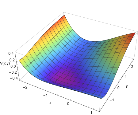
Figure 1: Morse-like potential in two dimensions.

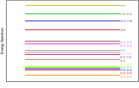
Figure 2: Energy spectrum.

By observing both the Table I and the Figure 2, one can note that there are some interesting results in the spectrum. First of all, we observe that this potential presents a finite number of allowed bound states, which is not a surprise, since this already happens in the case of the one-dimensional Morse potential (even in the case with position-dependent masses). However, in the case analyzed, there are inversions of energies where sates labeled with higher quantum numbers present lower energies than states with lower quantum numbers, as happens in the case of atoms with somewhat great atomic numbers. On the other hand, beyond the some expected degeneracies, we observe that there is a eight-fold degenerated stated (the seventh exited one). In this case we checked that one shall have an accidental degeneracy, since we checked that changing slightly some potential parameters this degeneracy disappears, becoming a quasi-degeneracy.

IV Final comments

In this work, we present a general construction of a class of a two-dimensional PDM systems in Cartesian coordinates, analyzing an exactly solvable case and discussing its ordering ambiguity and some of their properties. We extend the idea to the problem where ones deal with increasing mass Morse-like. In this case we obtain the exact wave-functions and energies for a complete set of eigenstates. Since the energy of the bound states come from a transcendental equation, involving the quantum numbers of a pair of one-dimensional equations, we discovered that this system presents a behavior which emulates the inversion of excited states usually seen in atoms with high atomic numbers. Moreover, an interesting accidental degeneracy appeared. Finally, it is important to remark that one could use this exactly solvable system in order to construct more realistic ones by using their solution in perturbative approaches.

- (1) Y. Alhassid, Rev. Mod. Phys. 72 (2000) 895.
- (2) M. A. Kastner, Rev. Mod. Phys. 64 (1992) 849.
- (3) A. R. Wright, M. Veldhorst, Phys. Rev. Lett. 111 (2013) 9, 096801.
- (4) G. Anatoly, Phys. Rev. B 91 (2015) 20, 205105.
- (5) Y. Li, A. Kundu, F. Zhong, and B. Seradjeh, Phys. Rev. 90 (2014) 12, 121401.
- (6) B. Wahlstrand, I. I. Yakimenko, K.-F. Berggren, Phys. Rev. E 89 (2014) 6, 062910.
- (7) P. Tighineanu, M. L. Andersen, A. S. Sorensen, S. Stobbe, and P. Lodahl, Phys. Rev. Lett. 113 (2014) 043601.
- (8) M. Lozada-Cassou, S. H. Dong, and J. Yu, Phys. Lett. A 331 (2004) 45.
- (9) A. G. M. Schmidt, A. D. Azeredo, and A. Gusso, Phys. Lett. A 372 (2008) 2774.
- (10) D. J. BenDaniel and C. B. Duke, Phys. Rev. B 152 (1966) 683.
- (11) T. Gora and F. Williams, Phys. Rev. 177 (1969) 1179.
- (12) G. Bastard. Phys. Rev. B 24 (1981) 5693.
- (13) O. Von Roos, Phys. Rev. B 27 (1983) 7547.
- (14) Q. G. Zhu and H. Kroemer, Phys. Rev. B 27 (1983) 3519.
- (15) T. L. Li and K. J. Kuhn, Phys. Rev. B 47 (1993) 12760.
- (16) F. S. A. Cavalcante, R. N. Costa Filho, J. Ribeiro Filho, C. A. S. de Almeida, and V. N. Freire, Phys. Rev. B 55 (1997) 1326.
- (17) A. de Souza Dutra and J. A. de Oliveira, J. Phys. A: Math Theor. 42 (2009) 025304.
- (18) J. R. Shewell, Am. J. Phys. 27 (1959) 16.
- (19) J. C. Slater, Phys. Rev. 76 (1949) 1592.
- (20) J. M. Luttinger and W. Kohn, Phys. Rev. 97 (1955) 869.
- (21) G. H. Wannier, Phys. Rev. 52 (1957) 191.
- (22) Ó. Rojo and J. S. Levinger, Phys. Rev. 123 (1961) 2177.
- (23) M. Razavy, G. Field, and J. S. Levinger, Phys. Rev. 125 (1962) 269.
- (24) G. Bastard, Wave Mechanics Applied to Semiconductor Heterostructres, Les Éditions de Physique, Les Ullis, 1992.
- (25) C. Weisbuch and B. Vinter, Quantum Semiconductor Heterostructures, Academic Press, New York, 1993.
- (26) C. C. Wu, J. Sun, F. J. Huang, Y. D. Li, W. M. Liu, Europhys. Lett. 104 (2013) 27004.
- (27) M. Benito, A. Gómez-León, V .M. Bastidas, T. Brandes, and G. Platero, Phys. Rev. B 90 (2014) 20, 205127.
- (28) J. Gong and Qing-hai Wang, Phys. Rev. A 91 (2015) 4, 042135.
- (29) A. de Souza Dutra and C. A. S. de Almeida, Phys. Lett. A 275 (2000) 25.
- (30) C. Quesne and V. M. Tkachuk, J. Phys. A 37 (2004) 426.
- (31) J. F. Carinena, M. F. Ranada, and M. Santander, Ann. Phys. 322 (2007) 434.
- (32) A. Ganguly and L. M. Nieto, J. Phys. A 40 (2007) 7265.
- (33) S. Choi, K. M. Galdamez, and B. Sundaram, Phys. Lett. A 374 (2010) 3280.
- (34) A. Arda, R. Sever, and C. Tezcan, Phys. Scripta 79 (2009) 015006.
- (35) A. Ganguly and A. Das, J. Math. Phys. 55 (2014) 11, 112102.
- (36) A. de Souza Dutra, J. Phys. A 39 (2006) 203.
- (37) A. de Souza Dutra, M. B. Hott, and C. A. S. Almeida, Europhys. Lett. 62 (2003) 8.
- (38) A. G. M. Schmidt, Phys. Lett. A 353 (2006) 459.
- (39) C. Quesne, J. Math. Phys. 49 (2008) 022106; J. Phys. A 40 (2007) 13107; Ann. Phys. 321 (2006) 1221.
- (40) S. M. Ikhdair and R. Sever, J. Mol. Str. Theochem 885 (2008) 13.
- (41) A. Schulze-Halberg, Int. J. Mod. Phys. A 22 (2007) 1735; 21 (2006) 4853; 21 (2006) 1359.
- (42) J. F. Carinena, M. F. Ranada and M. Santander, Ann. Phys. 322 (2007) 2249.
- (43) A. Ganguly and L. M. Nieto, J. Phys. A 40 (2007) 7265.
- (44) B. Roy, Mod. Phys. Lett. B 20 (2006) 1033.
- (45) O. Mustafa and S. H. Mazharimousavi, J. Phys. A 41 (2008) 244020; 39 (2006) 10537.
- (46) T. Tanaka, J. Phys. A 39 (2006) 219.
- (47) R. Koc, M. Koca, and G. Shaninoglu, Eur. Phys. J. B 48 (2005) 583.
- (48) U. Gunther, F. Stefani, and M. Znojil, J. Math. Phys. 46 (2005) 063504.
- (49) G. Chen, Chin. Phys. 14 (2005) 460.
- (50) G. Chen and Z. D. Chen, Phys. Lett. A 331 (2004) 312.
- (51) A. A. Stahlhofen, J. Phys. A 37 (2004) 10129-10138,
- (52) B. Bagchi, P. Gorain, C. Quesne, and R. Roychoudhury, Mod. Phys. Lett. A 19 (2004) 2765-2775,
- (53) K. Bencheikh, K. Berkane, and S. Bouizane, J. Phys. A 37 (2004) 10719.
- (54) J. A. Yu and S. H. Dong, Phys. Lett. A 325 (2004) 194.
- (55) C. Quesne and V. M. Tkachuk, J. Phys. A 37 (2004) 4267.
- (56) Y. C. Ou, Z. Q. Cao, and Q. H. Shen, J. Phys. A 37 (2004) 4283.
- (57) R. Koc and H. Tutunculer, Annalen der Physik 12 (2003) 684.
- (58) A. D. Alhaidari, Phys. Rev. A 66 (2002) 042116.
- (59) B. Roy and P. Roy, J. Phys. A 35 (2002) 3961.
- (60) S. Ramgoolam, B. Spence, and S. Thomas, Nucl. Phys. B 703 (2005) 236.
- (61) A. de Souza Dutra, M. B. Hott, and V. G. C. S. dos Santos, Europhys. Lett. 71 (2005) 166.
- (62) B. K. Cheng and A. de Souza Dutra, Phys. Lett. A 123 (1987) 105.
- (63) A. de Souza Dutra and B. K. Cheng, Phys. Rev. A 39 (1989) 5897.
- (64) A. de Souza Dutra, C. F. de Souza, and L. C. de Albuquerque, Phys. Lett. A 156 (1991) 371.
- (65) M. S. Abdalla and J. R. Choi, Ann. Phys. 322 (2007) 2795.
- (66) A. de Souza Dutra and J. A. de Oliveira, J. Phys. A: Math. Theor. 42 (2009) 025304.
- (67) A. G. M. Schmidt, J. Phys. A: Math. Theor. 42 (2009) 245304.
- (68) O. Mustafa, J. Phys. A: Math. Theor. 43 (2010) 385310.
- (69) A. G. M. Schmidt, Phys. A 391(2012) 3792.
- (70) A. G. M. Schmidt, L. Portugal, and A. L. de Jesus, J. Math. Phys. 56 (2015) 012107.