Inertial and dimensional effects on the instability of a thin film

Abstract

We consider here the effects of inertia on the instability of a flat liquid film under the effects of capillary and intermolecular forces (van der Waals interaction). Firstly, we perform the linear stability analysis within the long wave approximation, which shows that the inclusion of inertia does not produce new regions of instability other than the one previously known from the usual lubrication case. The wavelength, $\lambda_{m}$, corresponding to he maximum growth, $\omega_{m}$, and the critical (marginal) wavelength do not change at all. The most affected feature of the instability under an increase of the Laplace number is the noticeable decrease of the growth rates of the unstable modes. In order to put in evidence the effects of the bidimensional aspects of the flow (neglected in the long wave approximation), we also calculate the dispersion relation of the instability from the linearized version of the complete Navier-Stokes (N–S) equation. Unlike the long wave approximation, the bidimensional model shows that $\lambda_{m}$ can vary significantly with inertia when the aspect ratio of the film is not sufficiently small. We also perform numerical simulations of the nonlinear N–S equations and analyze to which extent the linear predictions can be applied depending on both the amount of inertia involved and the aspect ratio of the film.

sectioning  

Inertial and dimensional effects on the instability of a thin film

 

1 Introduction

The stability of thin films on substrates has been for a long time a basic subject of research, not only because of the numerous technological applications, including coatings, adhesives, lubricants, and dielectric layers, but also because of their fundamental interest (Craster and Matar, 2009; Eggers, 1997; Oron et al., 1997). The dewetting of thin liquid films is the process of destabilization of such films which leads to the formation of drops. It is generally observed when the supported liquid film is placed on a substrate under partial wetting conditions, and subject to destabilizing intermolecular forces. For a homogeneous isotropic liquid on a uniform solid substrate, two main dewetting processes are known: (i) the nucleation of holes at defects or dust particles, and (ii) the amplification of perturbations at the free surface (e.g., capillary waves) under the destabilizing effect of long-range intermolecular forces in the so-called spinodal dewetting (Thiele, 2003; Thiele et al., 2001, 1998). Although the distinction between these two dewetting processes is well established in the literature, there is still a lot of debate about which of these mechanisms is actually observed in a given experiment.

In this context, lubrication approximations to the full Navier-Stokes equations have shown to be extremely useful for investigating the dynamics and instability of thin liquid films on substrates, including the motion and instabilities of their contact lines (Oron et al., 1997). The theoretical treatment of the coating problem is greatly simplified if the film is so thin that the lubrication approximation can be employed. When this modeling is valid, it is possible to determine the velocity field of the liquid as a function of the film thickness, and the problem reduces to the solution of a nonlinear evolution equation for the thickness profile of the film. To leading order, at low speeds, the dynamics is controlled by a balance among capillarity, viscosity, and intermolecular forces, without inertia playing a role. This approach has achieved considerable success in dealing with the solution of this class of problems (Colinet et al., 2007).

However, in some applications such as the dewetting of nano-scale thin metallic films on hydrophobic substrates, the effects related to inertia and the shortcomings of the lubrication approximation assumptions (requiring small slopes and consequently small contact angles) appear to have a crucial influence on the dynamics and morphology of the film (González et al., 2013). Experimental studies of unstable thin films coating solids have shown significant differences in the patterns that develop when fluid instabilities lead to the formation of growing dry regions on the solid. The effects of inertia on the instability have been studied previously in other problems, for example for a film flowing down an incline (Lopez et al., 1997), the breakup of a liquid filament sitting on a substrate (Ubal et al., 2014), and several other configurations (Hocking and Davis, 2002). However, these problems do not include explicitly the effects of the intermolecular interaction between the molecules of the liquid and those of the solid. Here, we consider it by using integrated Lennard-Jones forces, which lead to the disjoining pressure that entails the power dependence on the fluid thickness (Kargupta et al., 2004). In the present context, the occurrence and nature of both inertia and bidimensional effects in the liquid film on the solid substrate is of interest, not only for fundamental research, but also for technological applications.

The solutions of problems under the lubrication approximation is usually limited to speeds low enough to give small capillary and Reynolds numbers. The extension of the theory to higher speeds introduces inertia into the problem, and, even in the case of thin films, the analysis may become much more difficult. The great simplification previously found by the application of the lubrication theory no longer exists; instead, the system is governed by the coupling of a nonlinear partial differential equation for the velocity field, and an evolution equation for the thickness profile. It is possible, however, to find a class of problems in which inertial effects can be assessed within the long wave framework. In this work we are concerned with the instability of a flat liquid film extended over a solid plane, and subject to intermolecular forces between the liquid and the solid substrate. Then, the film evolution is studied by considering viscous, surface tension, and intermolecular forces, with special emphasis on the effect of inertia in the development of the instability.

2 Intermolecular forces in the hydrodynamic description

We consider a thin liquid film of thickness $h_{0}$, which spans infinitely in the $x$-direction (the system is invariant in the $y$-direction, i.e. plane flow conditions prevail), and rests on a solid plane at $z=0$ (see Fig. 1a). Here, we will consider the instability of this initially flat film under the action of surface tension and intermolecular forces, acting both at the free surface of the film with instantaneous thickness $h(x,t)$. Thus, the hydrodynamic evolution is governed by the Navier-Stokes equation and the incompressibility condition,

$$\rho\left(\partial_{t}\mathbf{v}+\mathbf{v}\cdot\nabla\mathbf{v}\right)=-\nabla p+\mu\Delta\mathbf{v},\qquad\nabla\cdot\mathbf{v}=0$$ (1)

where $\rho$ is the liquid density, $\mu$ its viscosity, $p$ the pressure and $\mathbf{v}=(u,w)$ the velocity field. At the substrate ($z=0$), we apply the no-slip and non-penetration conditions. At the free surface, $z=h(x,t)$, we have the usual kinematic condition and normal stress equilibrium given by

$$p=-\Pi-\gamma\cal{C}$$ (2)

where $\gamma$ is the surface tension, $\cal{C}$ the curvature of the surface, and

$$\Pi(h)=\kappa f(h)=\kappa\left[\left(\frac{h_{\ast}}{h}\right)^{n}-\left(\frac{h_{\ast}}{h}\right)^{m}\right],$$ (3)

is the disjoining pressure. Here, $\kappa$ is a constant with units of pressure (related to the Hamaker constant of the system), the exponents satisfy $n>m>0$, and $h_{\ast}$ is the equilibrium thickness (of the order of some nanometers). This surface force is a consequence of the interaction among the molecules in the three phases present in the problem, namely the liquid of the film, the solid substrate and the surrounding gas. Note that at equilibrium, i.e. when $h=h_{0}=const.$, the film has a uniform pressure $p_{0}=-\Pi(h_{0})>0$, since $\Pi(h_{0})<0$ for $h_{0}>h_{\ast}$.

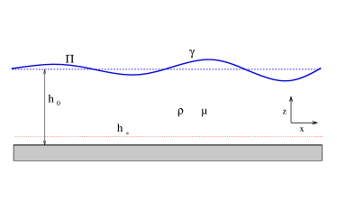
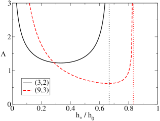
Figure 1: (a) Schematic diagram of the problem. (b) Parameter $\Lambda$ as given by Eq. (24) as a function of the ratio between the equilibrium thickness, $h_{\ast}$, and the film thickness, $h_{0}$, for two pairs of the exponents $(n,m)$. The vertical dotted lines correspond to $g_{0}=0$, i.e. $h_{\ast}=h_{0}\,(m/n)^{1/(n-m)}$.

3 Long wave approximation

In this approximation it is assumed that the film thickness, $h_{0}$, is much smaller than the characteristic horizontal length of the problem. Since the film extends to infinity, we assume that there exists a typical length associated with the wavelength of the perturbations, namely $\ell$. The definition of $\ell$ will be made more precise below. Subsequently, for $\varepsilon=h_{0}/\ell\ll 1$, we can simplify Eq. (1) under the long wave approximation assumptions retaining inertial terms in the form

$$-\frac{\partial p}{\partial x}+\mu\frac{\partial^{2}u}{\partial z^{2}} = \rho\left(\frac{\partial u}{\partial t}+u\frac{\partial u}{\partial x}+w\frac{\partial u}{\partial z}\right)$$ (4)

$$-\frac{\partial p}{\partial z} = 0$$ (5)

$$\frac{\partial u}{\partial x}+\frac{\partial w}{\partial z} = 0.$$ (6)

The boundary conditions for these equations are as follows. At $z=0$, we impose no penetration and no slip at the substrate,

$$w=0,\qquad u=0.$$ (7)

At the liquid-gas interface ($z=h$), we have zero shear stress,

$$\frac{\partial u}{\partial z}=0,\qquad$$ (8)

as well as the kinematic condtion,

$$\frac{\partial h}{\partial t}+u\frac{\partial h}{\partial x}=w,$$ (9)

and the Laplace relation for the capillary pressure

$$p(h)=-\gamma\frac{\partial^{2}h}{\partial x^{2}}-\kappa f(h),$$ (10)

From Eq. (5) we see that the pressure, $p$, is $z$-independent, and then $p$ is only a function of $h$, $p=p(h)$. Thus, we have that the $x$-derivative of $p$ in Eq. (4) is given by

$$\frac{\partial p}{\partial x}=-\gamma\frac{\partial^{3}h}{\partial x^{3}}-\kappa f^{\prime}(h)\frac{\partial h}{\partial x}.$$ (11)

The continuity equation, Eq. (6), is conveniently satisfied by introducing the stream function $\psi(x,z,t)$ defined by

$$u=\frac{\partial\psi}{\partial z},\qquad w=-\frac{\partial\psi}{\partial x}.$$ (12)

Therefore, Eqs. (4) and (9) in terms of $\psi$ are given by

$$\mu\frac{\partial^{3}\psi}{\partial z^{3}}=-\gamma\frac{\partial^{3}h}{\partial x^{3}}-\kappa f^{\prime}(h)\frac{\partial h}{\partial x}+\rho\left(\frac{\partial^{2}\psi}{\partial z\partial t}+\frac{\partial\psi}{\partial z}\frac{\partial^{2}\psi}{\partial x\partial z}-\frac{\partial\psi}{\partial x}\frac{\partial^{2}\psi}{\partial z^{2}}\right),$$ (13)

$$\frac{\partial h}{\partial t}+\frac{\partial\psi(x,h,t)}{\partial x}=0.$$ (14)

The boundary conditions, given by Eqs. (7) and (8), in terms of $\psi$ are:

$$\left.\psi\right|_{z=0}=0,\qquad\left.\frac{\partial\psi}{\partial z}\right|_{z=0}=0,\qquad\left.\frac{\partial^{2}\psi}{\partial z^{2}}\right|_{z=h}=0.$$ (15)

3.1 Linear stability analysis within long wave approximation

The equilibrium state is given by $h=h_{0}$, and for small-amplitude perturbations, the height and stream function can be written in the form

$$h=h_{0}\left(1+Ae^{\omega t+ikx}\right),\qquad\psi=A\psi_{1}(z)e^{\omega t+ikx},$$ (16)

where $A$ is the small amplitude of the perturbation, and unstable (stable) modes correspond to $\omega>0$ ($\omega<0$). By replacing Eq. (16) into Eqs. (13) and (14), and retaining terms up to order one in $\varepsilon$, we have

$$\mu\frac{d^{3}\psi_{1}}{dz^{3}}=i\gamma h_{0}k^{3}-i\kappa h_{0}f^{\prime}(h_{0})k+\rho\,\omega\frac{d\psi_{1}}{dz},$$ (17)

$$\omega+ik\psi_{1}(h_{0})=0,$$ (18)

with the boundary conditions

$$\left.\psi_{1}\right|_{z=0}=0,\qquad\left.\frac{d\psi_{1}}{dz}\right|_{z=0}=0,\qquad\left.\frac{d^{2}\psi_{1}}{dz^{2}}\right|_{z=1}=0.$$ (19)

Now, we define the horizontal length scale, $\ell$, by choosing $\kappa f^{\prime}(h_{0})=\gamma/\ell^{2}$, so that it turns out

$$\ell=\sqrt{\frac{\gamma}{\kappa f^{\prime}(h_{0})}}=\sqrt{\frac{\gamma h_{0}}{\kappa g_{0}}},$$ (20)

where

$$g_{0}=h_{0}f^{\prime}(h_{0})=-n\left(\frac{h_{\ast}}{h_{0}}\right)^{n}+m\left(\frac{h_{\ast}}{h_{0}}\right)^{m}.$$ (21)

Since $n>m$ and $h_{0}>h_{\ast}$, we have $g_{0}>0$. Note that we are here including in $\ell$ all the effects related with the magnitude of the intermolecular forces given by $\kappa$. In fact, this constant is usually related in the literature with the contact angle, $\theta$, which appears at the contact regions formed when the film thins up to $h_{\ast}$, and characterizes the partial wetting of the substrate. It is found that the following simple relationship holds (Oron et al., 1997; Schwartz and Eley, 1998; Diez and Kondic, 2007)

$$\kappa=\frac{\gamma(1-\cos\theta)}{Mh_{\ast}},$$ (22)

where $M=(n-m)/((n-1)(m-1))$. Thus, the characteristic length scale becomes

$$\ell=\sqrt{\frac{Mh_{0}h_{\ast}}{(1-\cos\theta)g_{0}}},$$ (23)

so that this length includes all the parameters determining the problem, except for $\gamma$ and $\mu$ which yield the time scale (see Eq. (26) below). In Fig. 1b, we show how the dimensionless combination

$$\Lambda=\sqrt{1-\cos\theta}\frac{\ell}{h_{0}}=\sqrt{\frac{Mh_{\ast}}{g_{0}h_{0}}}$$ (24)

depends on the ratio $h_{\ast}/h_{0}$ for two fixed values of the exponents pair $(n,m)$. Interestingly, very small values of $h_{\ast}$ as well as $h_{\ast}$ close to $h_{0}\,(m/n)^{1/(n-m)}$ yield very large values of $\ell/h_{0}$ for given contact angle, $\theta<\pi/2$.

Consequently, a convenient non-dimensional version of the problem for the long wave approximation is given by the following scaling

$$X=\frac{x}{\ell},\quad Z=\frac{z}{h_{0}},\quad H=\frac{h}{h_{0}},\quad T=\frac{\varepsilon^{3}}{\tau}t,\quad\Psi_{1}=\frac{\tau}{\varepsilon^{3}\ell}\psi_{1},\quad K={\ell}k,\quad\Omega=\frac{\tau}{\varepsilon^{3}}\omega,$$ (25)

where

$$\tau=\frac{\mu\ell}{\gamma}$$ (26)

is the time scale. Under these definitions, Eqs. (17) and (18) become

$$\frac{d^{3}\Psi_{1}}{d{Z}^{3}}+q^{2}\frac{d\Psi_{1}}{dZ}=i{K}({K}^{2}-1),$$ (27)

$$\Omega+i{K}\Psi_{1}(1)=0,$$ (28)

where

$$q^{2}=-La^{\ast}\,\Omega,$$ (29)

with

$$La^{\ast}=La\,\varepsilon^{5},$$ (30)

and

$$La=\frac{\rho\gamma\ell}{\mu^{2}}$$ (31)

being the Laplace number. The latter dimensionless number considers the effects of all the forces playing a role in the flow, namely, inertial (characterized by $\rho$), viscous (characterized by $\mu$), surface (characterized by $\gamma$) and intermolecular forces (characterized by $\ell$).

The solution of Eq. (27) has the form

$$\Psi_{1}=iK({K}^{2}-1)\frac{qZ+\sin(q-qZ)\sec Z-\tan q}{q^{3}},$$ (32)

which allows one to obtain the dispersion relation from Eq. (28) as

$$\frac{\Omega}{{K}^{2}\left({K}^{2}-1\right)}=\frac{q-\tan q}{q^{3}}.$$ (33)

In the limit $q\rightarrow 0$, this expression tends to the purely viscous solution,

$$\Omega_{vis}=\frac{{K}^{2}(1-{K}^{2})}{3},$$ (34)

which is obtained in the inertialess case (Diez and Kondic, 2007) for $La=0$. Note that the dimensionless critical (marginal) wavenumber is equal to unity for the viscous case, i.e. $K_{c}=1$, so that Eq. (34) shows instability for $K<1$. This is because the choice of the in-plane characteristic length, $\ell$, the inverse of the dimensional critical wavenumber (Nguyen et al., 2012).

By dividing Eq. (33) by $q^{2}$ and using Eq. (29), we may define the parameter $r$ as

$$r\equiv\frac{1}{La^{\ast}\,{K}^{2}({K}^{2}-1)},$$ (35)

and then, the possible values of $q$ for given $K$, are given by the roots of

$$r=\frac{\tan q-q}{q^{5}}.$$ (36)

In what follows, we will consider only real values of $K$. Thus, the allowed values of $r$ are $r<r_{max}=-4/La^{\ast}$ for $K<1$, and $r>0$ for $K>1$ (see Eq. (35) and Fig. 2a). In the region $K<1$ and $r<r_{max}$ there exist two different values of $K$ for a given $r$, and so they share the same growth rate, $\Omega$. At $r=r_{max}$ we have $K=K_{m}^{1D}=1/\sqrt{2}$. Instead, in the region $K>1$ and $r>0$, each mode $K$ has a unique and different $r$, and consequently, $\Omega$.

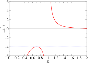
(a) $La^{\ast}r$ vs. $K$

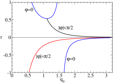
(b) $r$ vs. $q_{0}$

Figure 2: (a) Relationship between $La^{\ast}r$ and $K$ as given by Eq. (35). The dashed line is $r=-4/La^{\ast}$. (b) Possible values of $r$ as a function of $q_{0}$. The blue lines correspond to $\varphi=0$, the red one to $\varphi=\pi/2$ and the black one to $\varphi\neq$ const. (see Fig. 3a).

In order to analyse the possible values of $\Omega$ in each region, it is convenient to introduce the notation

$$q=q_{0}e^{i\varphi},$$ (37)

so that the complex growth rate is

$$\Omega=\Omega_{r}+i\,\Omega_{i}=-\frac{q_{0}^{2}}{La^{\ast}}e^{2i\varphi}.$$ (38)

For $\Omega_{r}=\Re(\Omega)>0$ ($<0$) we have unstable (stable) modes, and for $\Omega_{i}=\Im(\Omega)\neq 0$ we have spatially oscillating modes. Therefore, we consider the imaginary and real parts of Eq. (36), which read as

$$\Re(r)=F(q_{0},\varphi)=\left[-\Phi\cos 4\varphi+\sin(2q_{0}\cos\varphi)\cos 5\varphi+\sinh(2q_{0}\sin\varphi)\sin 5\varphi\right]/\Delta,$$ (39)

$$\Im(r)=G(q_{0},\varphi)=\left[\Phi\sin 4\varphi-\sin(2q_{0}\cos\varphi)\sin 5\varphi+\sinh(2q_{0}\sin\varphi)\cos 5\varphi\right]/\Delta,$$ (40)

where

$$\Phi = 2q_{0}\cos\left(q_{0}e^{-i\varphi}\right)\cos\left(q_{0}e^{i\varphi}\right),$$ (41)

$$\Delta = q_{0}^{5}(\cos[2q_{0}\cos\varphi]+\cosh[2q_{0}\sin\varphi]).$$ (42)

Since $r$ is real, the solutions of Eq. (36) must have $\Im(r)=0$. Two trivial roots of this function are $\varphi=0$ and $|\varphi|=\pi/2$. However, it is possible to find roots also along a curve in the $(q_{0},\varphi)$ plane given implicitly by the function $G(q_{0},\varphi)=0$ (see Fig. 3a).

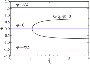
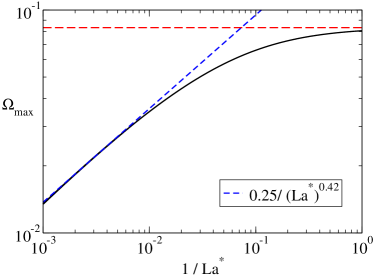
Figure 3: (a) Curves in the $(q_{0},\varphi)$ plane along which $\Im(r)=0$. (b) Maximum growth rate as a function of ${La^{\ast}}^{-1}$. The horizontal dashed line corresponds to $\Omega_{vis,max}=1/12$.

For $|\varphi|=\pi/2$ we find unstable real modes with growth rates given by (see Eq. (38))

$$\Omega=\Omega_{r}=\frac{q_{0}^{2}}{La^{\ast}}>0,$$ (43)

where $q_{0}$ is now given by the implicit relation

$$r(\pm i\,q_{0})=F(\pm i\,q_{0},\pm\pi/2)=\frac{\tanh q_{0}-q_{0}}{q_{0}^{5}}.$$ (44)

The function $r(\pm i\,q_{0})$ is plotted in with red lines in Fig. 2b. Since $r<0$ for all $q_{0}$, this branch corresponds to $K<1$.

Instead, for $\varphi=0$, we obtain stable real modes whose growth rates are given by (see Eq. (38))

$$\Omega=\Omega_{r}=-\frac{q_{0}^{2}}{La^{\ast}}<0,$$ (45)

where $q_{0}$ is obtained through the implicit relation (see blue lines in Fig. 2b )

$$r(q_{0})=F(q_{0},0)=\frac{\tan q_{0}-q_{0}}{q_{0}^{5}}.$$ (46)

The function $r(q_{0})$ is plotted in with blue lines in Fig. 2b. Since $r$ changes sign at $q_{0}=\pi/2$, the upper branch corresponds to $K>1$, while the lower one to $K<1$. Moreover, these branches are related to monotonically damped modes.

The implicit relation $G(q_{0},\varphi)=0$ (plotted as the black curve in Fig 3a) allows to obtain $r(q_{0}e^{i\varphi})$ as a function of $q_{0}$ (see black curve in Fig. 2b). This branch appears as a bifurcation point of the the upper branch $\varphi=0$, with coordinates $B=(r_{b},q_{0,b})=(1.1127,0.5367)$. Since $|\varphi|\neq 0,\pm\pi/2$ we have complex values of the growth rate, $\Omega$, as determined by Eq. (38). Moreover, since $|\varphi|<\pi/2$, $\Omega_{r}$ is always negative and it corresponds to oscillating stable (damped) modes. Besides, it turns out that $r>0$, so that these modes belong the region $K>1$.

As a result, only the branch $|\varphi|=\pi/2$ includes unstable modes, which are in the region $k<1$ and $r<r_{max}$ of Fig. 2a. The mode with maximum (real) growth rate, $\omega_{max}$, is given by $r=r_{max}<0$ for a given $La^{\ast}$ and is located at the intersection with the line $|\varphi|=\pi/2$ in Fig. 2b. In fact, for given $La^{\ast}$ we solve

$$\frac{\tanh q_{0,max}-q_{0,max}}{q_{max}^{5}}=-\frac{4}{La^{\ast}},$$ (47)

for $q_{0,max}$ and obtain $\Omega_{max}=-q_{0,max}^{2}/La^{\ast}$. The result is shown in Fig. 3b, where it is observed how $\Omega_{max}$ tends to the viscous value, namely $\Omega_{vis,max}=1/12$ (see Eq.(34)), as $La^{\ast}\rightarrow 0$. It is also shown that the behavior for large $La^{\ast}$ corresponds to a decreasing growth rate as a power law with exponent close to $0.42$. Similar decreasing trends of the growth rates due to inertial effects have also been found in other problems (Oron et al., 1997; Ubal et al., 2014).

Figure 3b also shows that the line $r=r_{max}$ is also intersected by the $\varphi=0$ line. Since it corresponds to monotonically damped perturbations in the region $0<k<1$, this implies that the maximum damping for the stable mode occurs at the same $k$ than the unstable modes in the $|\varphi|=\pi/2$.

Note that unstable monotonically growing modes are only possible for $k<1$, so that neither the critical wavelength nor that of maximum growth rate are affected by the value of $La^{\ast}$. However, the maximum growth rate itself is altered by the relative weight of inertial effects with respect to viscosity and capillarity. Therefore, the Laplace number is relevant when discussing time scales and growth rates, but not for critical or dominant wavelengths.

The modes with $k>1$ correspond to the $r>0$ region and are always stable as it is the case in the usual viscous lubrication approximation, but we want now to analyze whether there is any change in their behaviour when inertia effects are included. First, note that for each $k>1$, there is a single value of $r>0$ (see Fig. 2a). This value of $r$ could yield either $\varphi=0$ (blue line, upper branch) or $|\varphi|<\pi/2$ at the black line in Fig. 2b. Two different situations ensue. If $r>r_{b}$, the solutions are on the $\varphi=0$ (blue) line, i.e. the modes are monotonically damped, and two different values of $q$ are admissible: one smaller and the other larger than $q_{0,b}$. At the point $B=(r_{b},q_{0,b})$, both roots degenerate into a single one. For $0<r<r_{b}$, the roots are found along the black line, and the modes are oscillatory and damped. From Eq. (35), we find the wavenumber corresponding to point $B$ as given by

$$K_{b}=\sqrt{\frac{1}{2}+\sqrt{\frac{1}{4}+\frac{1}{La^{\ast}\,r_{b}}}}.$$ (48)

Thus, for $1<K<K_{b}$ there are two damped real modes, while for $K>K_{b}$ ($r<r_{b}$) two oscillatory (complex) damped modes are possible with increasing frequency oscillations and stronger damping as $K$ increases.

In summary, the condition $\Im(r)=0$ (i.e., $r$ real) yield three types of lines in the $(q_{0},\varphi)$ plane, which can be classified as:

1. $\varphi=0$, which yields stable damped (real) modes,

2. $|\varphi|=\pi/2$, which can be related to unstable purely growing (real) modes, and

3. $\varphi\neq 0,\pi/2$, that will produce stable oscillatory modes in time, i.e. complex conjugate roots of $\Omega$.

The procedure to obtain the dispersion relation of the problem, i.e. $\Omega(K)$, for a fixed $La^{\ast}$ is as follows. Given a value $K$, we obtain the corresponding $r$ (see Eq. (35) and Fig. 2a). Then, with this value of $r$, we find $q_{0}$ (e.g. using Fig. 2b). In the case of complex roots (black line) the corresponding value of $\varphi$ is a consequence of requiring that $\Im(r)=0$ in Eq. (40). Once this is done, we obtain the full spectrum of modes as shown in Fig. 4. The dashed lines correspond to $\Omega_{i}$ for the complex modes along the black line named C.

We observe in Fig. 4 that $La^{\ast}$ strongly modifies some features of the complete dispersion relation. For instance, it modifies the maximum, $\Omega_{max}$, in the unstable region ($K<1$, $\Omega_{r}>0$). Note that the product $La^{\ast}\Omega_{max}$ grows with $La^{\ast}$ because $\Omega_{max}$ decreases with $La^{\ast}$ with an exponent less than one (see Fig. 3b). Analogously, $La^{\ast}$ also affects the minimum in the stable region with $K<1$. For $K>1$, $La^{\ast}$ only modifies the value of $K_{b}$ (see Eq. (48)).

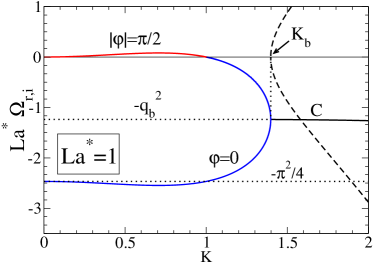
(a) $La^{\ast}=1$

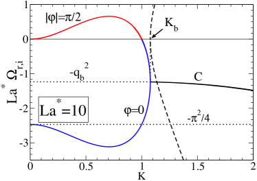
(b) $La^{\ast}=10$

Figure 4: Real (solid lines) and imaginary (dashed lines) parts of $\Omega=\Omega_{r}+i\Omega_{i}$ multiplied by $La^{\ast}$ as a function of the wavenumber $K$ for (a) $La^{\ast}=1$, and (b) $La^{\ast}=10$. The curves for $\Omega_{r}>0$ and $K<1$ (unstable region) correspond to $|\varphi|=\pi/2$, and those for $\Omega_{r}<0$ and $K<K_{b}$ (stable region for damped modes) correspond to $\varphi=0$

In Fig. 5 we show a more detailed comparison of the dispersion curves for several $La^{\ast}$’s, both on the real growth rates for unstable ($\Omega_{r}>0$) and stable ($\omega_{r}<0$) modes. Part a) shows that as $La^{\ast}$ increases the unstable modes have lower growth rates, but the wavenumber of the maximum growth is not altered, and remains at $K_{max}=1/\sqrt{2}$. For very small $La^{\ast}$, the viscous dispersion relation is rapidly approached (see Eq (34)). Figure 5b shows the stable region of the instability diagram ($K>1$). For $1<K<K_{b}$), there two branches of modes that decay exponentially, a characteristic of the instability which is lost in the viscous approximation. For $K>1$, the viscous solution, $\Omega_{vis}$, is a fairly good approximation if $K\lesssim K_{b}$, but fails for $K$ around $K_{b}$. Clearly, this solution cannot describe the oscillating modes for $K>K_{b}$.

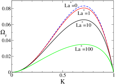
(a) Unstable modes

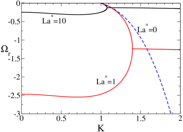
(b) Stable modes

Figure 5: Dispersion relations, $\Omega_{r}(k)$, for some values of $La^{\ast}$: (a) stable region, and (b) unstable region. The dashed line for $La^{\ast}=0$ is given by Eq. (34).

4 Bidimensional flow: Linear stability analysis

We consider here the full Navier-Stokes equation, Eq (1), in its dimensional form without the long wave approximation assumptions, i.e. the ratio $\varepsilon$ is not necessarily small now. Therefore, the small perturbations of the free surface are done on the velocity and pressure fields, and are expressed in terms of normal modes with a wavenumber $\mathbf{k}=(k_{x},0,0)$ parallel to the substrate. Thus, we have

$$\delta\mathbf{v} = \mathbf{v}(z)\,e^{i\mathbf{k}\cdot\mathbf{r}+\omega t},$$

$$p = p_{0}+\delta p=p_{0}+p_{1}(z)\,e^{i\mathbf{k}\cdot\mathbf{r}+\omega t},$$ (49)

$$h = h_{0}+\delta h=h_{0}+\zeta\,e^{i\mathbf{k}\cdot\mathbf{r}+\omega t},$$

where $\mathbf{v}=(u(z),0,w(z))$ and $\delta h$ is the Lagrangian displacement of the free surface. Note that, for small perturbations, we have $\zeta=w(1)/\omega$. Then, the Navier–Stokes equation at first order in the perturbations becomes

$$\rho\,\partial_{t}\delta\mathbf{v}=-\nabla\delta p+\mu\Delta\delta\mathbf{v}.$$ (50)

Since we assume incompressible flows, $i\mathbf{k}\cdot\mathbf{v}=-Dw$, where $D\equiv d/dz$. In order to reduce the number of variables, we eliminate the pressure terms, by taking the $z$ component of the $\nabla\times\nabla\times$Eq. (50). After some calculations, we obtain

$$(D^{2}-k^{2}_{x})(D^{2}-s^{2}\,k^{2})w=0$$ (51)

where $k=k_{x}$, and

$$s^{2}\equiv 1+\,\omega/(\nu k^{2}),$$ (52)

or equivalently

$$\omega=\left(s^{2}-1\right)\nu k^{2}.$$ (53)

The general solution of Eq (51) is

$$w=A_{1}\cosh(kz)+A_{2}\cosh(s\,kz)+A_{3}\sinh(kz)+A_{4}\sinh(s\,kz),$$ (54)

where the constants $A_{i}$ ($i=1,...,4$) are calculated by applying the following boundary conditions.

First, we impose the no flow condition through the rigid substrate,

$$\left.w\right|_{z=0}=0.$$ (55)

Second, we shall assume that there is no slip at the substrate, $\left.u\right|_{z=0}=0$. Since the flow is incompressible, then

$$\left.Dw\right|_{z=0}=0$$ (56)

Third, the tangential stresses at the free surface should be zero, $\left.\mathbf{k}\cdot{\cal S}\cdot\mathbf{e}_{z}\right|_{z=h_{0}}=0$, where ${\cal S}=-p\mathbf{I}+\mu\nabla\delta\mathbf{v}+\mu(\nabla\delta\mathbf{v})^{T}$ is the stress tensor. By replacing here the perturbed quantities, Eq. (4), we find

$$\left.(D^{2}+k^{2})w\right|_{z=h_{0}}=0,$$ (57)

Finally, the normal stress at the free surface must satisfy the generalized Laplace pressure jump,

$$\left.\mathbf{e}_{z}\cdot{\cal S}\cdot\mathbf{e}_{z}\right|_{z=h_{0}}=\gamma{\cal C}+\Pi,$$ (58)

where ${\cal C}=-k^{2}\zeta$ is the first order curvature of the perturbed free surface. Since

$$\zeta=\left.\frac{w}{\omega}\right|_{z=h_{0}},$$ (59)

we have

$$\left.(-p_{1}+2\mu Dw)\right|_{z=h_{0}}=\left.\frac{d\Pi}{dh}\right|_{h=h_{0}}\zeta-\gamma k^{2}\zeta$$ (60)

Notice that the term in $d\Pi/dh$ plays a role that is analogous to that of $\rho g$ in the Rayleigh–Taylor instability of a thin film. In order to obtain $p_{1}$ for this equation, we perform the scalar product of Eq. (50) by $\mathbf{k}$, and using Eq. (53) we find

$$p_{1}=\mu\left(\frac{D^{2}}{k^{2}}-s^{2}\right)Dw.$$ (61)

Then, by replacing this expression of $p_{1}$ at $z=h_{0}$ into Eq. (60), we finally write this boundary condition as

$$\left.\frac{\gamma}{\ell^{2}}(k^{2}\ell^{2}-1)\frac{w}{\omega}\right|_{z=h_{0}}=\left.\mu\left(\frac{D^{2}}{k^{2}}-2-s^{2}\right)Dw\right|_{z=h_{0}}$$ (62)

where $\ell$ is defined by Eq. (20).

From the above boundary conditions, Eqs. (55), (56), (57) and (62), it is possible to build up a matricial system to solve the four unknowns, $A_{i}$ ($i=1,...,4$). Its determinant must be zero to avoid a trivial solution. This condition leads to

$${K}^{3}\left[-4\left(s+s^{3}\right)+s\left(5+2s^{2}+s^{4}\right)\cosh({K}\varepsilon)\cosh(s\,{K}\varepsilon)-\right.$$

$$\left.\left(1+6s^{2}+s^{4}\right)\sinh({K}\varepsilon)\sinh(s\,{K}\varepsilon)\right]+$$

$$La\left({K}^{2}-1\right)\left[s\cosh(s\,{K}\varepsilon)\sinh({K}\varepsilon)-\cosh({K}\varepsilon)\sinh(s\,{K}\varepsilon)\right]=0,$$ (63)

with $K$ and $La$ defined in Eqs. (25) and (31), respectively.

This expression is the dispersion relation of the problem, since it implicitly gives $s$ as a function of $K$. The values of $\omega$ can be obtained through Eq. (53), which in dimensionless variables is

$$\Omega\,=\omega\tau=\frac{{K}^{2}}{\varepsilon^{3}La}(s^{2}-1).$$ (64)

It can be shown that Eq. (63) is identical to that obtained in Kargupta et al. (2004) if slipping at the substrate is neglected once we take into account that $\alpha$ and $\beta$ in their Eqs. (6) and (7) are $K\varepsilon$ and $s\,K\varepsilon$ respectively (our $s$ corresponds to their $q$).

In order to obtain the limit of Eq. (63) for $\varepsilon\ll 1$, note first that $q$ in Eq. (29) of the long wave model is related to $s$ in Eq. (52) by

$$q^{2}=(1-s^{2}){K}^{2}\varepsilon^{2},$$ (65)

and that $K\,\varepsilon=2\pi h_{0}/\lambda<<1$ in this limit. In order to keep a meaningful value of $q$, $|s|\gg 1$ is required, which means that $q\approx iKs\varepsilon$. Thus, with these ingredients in mind when analysing the limiting behavior of the dispersion relation given by Eq. (63), to the lowest meaningful order in $\varepsilon$, we find

$$La^{\ast}\,{K}^{2}({K}^{2}-1)(\tan q-q)=q^{5}$$ (66)

which is the same expression as given by the long wave model when Eqs. (35) and (36) are combined.

5 Comparison between long wave and bidimensional models

In this section we study the effects of $La$ and $\varepsilon$ on the dispersion relation for the unstable region as given by the one dimensional (1D) long wave approximation and the bidimensional (2D) model. For the 1D case, we focus on the solution of Eqs. (35) and (36) for $\varphi=\pi/2$, while for the 2D case we numerically solve Eq. (63) together with Eq. (64).

In Fig. 6 we show the comparison between 1D and 2D dispersion relations for given values of $La$ (columns) and $\varepsilon$ (rows). The inertial effects are shown along a given row (fixed $\varepsilon$), with the first column being a viscous dominated flow, and the fourth column corresponding to inertia dominated cases. For small $\varepsilon$, as in first row where $\varepsilon=0.1$, both dispersion relations are practically coincident for any value of $La$, as expected and shown analytically in Eq. (66). In general, the long wave model qualitatively predicts the same trends as the 2D model. However, for $\varepsilon$ as large as $\varepsilon=0.5$ (second row), the quantitative comparison certainly depends on $La$: the smaller $La$, the larger is the departure between both models, i.e. 2D effects become more important for flows with weak inertia. This effect is still more pronounced for larger $\varepsilon$ as seen in the third row for $\varepsilon=1$. Also note that, for fixed $La$, the position of the maximum shifts towards the left as $\varepsilon$ increases.

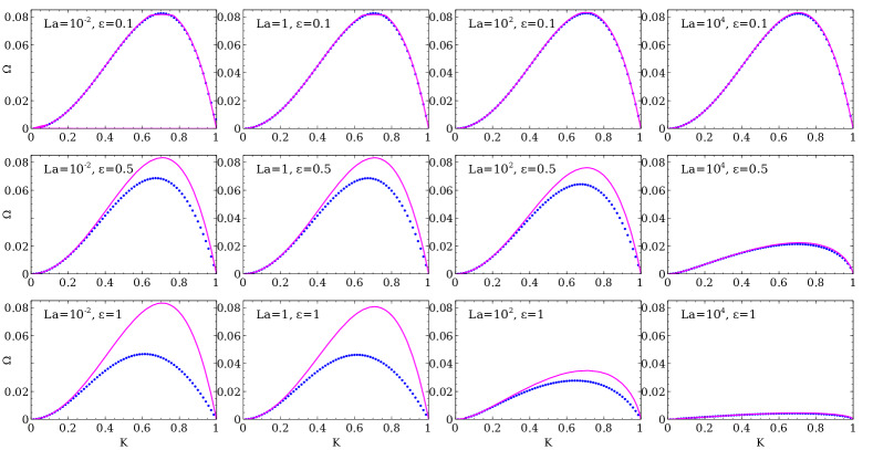
Figure 6: Dispersion relations, $\Omega$ as a function of $K$, for different values of $La$ and $\varepsilon$ for the linearized problem: 2D model (N–S solution, blue dots) and 1D long wave approximation with inertia (purple lines). For large $La$ (strong inertia) we obtain similar results for both models. For small $La$ (weak inertial effects) there are meaningful differences between both models (different $\varepsilon$’s)

We focus now on the behavior of the maximum of the dispersion relations, since its analysis provides interesting insight on the effects of both inertia and aspect ratio. While the behavior for the 1D model has been already described, the 2D model results can be obtained noticing that for $\Omega=\Omega_{max}$:

$$0=\frac{d\Omega(s,K)}{dK}=\frac{\partial\Omega}{\partial K}+\frac{\partial\Omega}{\partial s}\frac{ds}{dK}.$$ (67)

Since the dispersion relation satisfies $F(s,K)=0$, one can calculate

$$\frac{ds}{dK}=-\frac{\frac{\partial F}{\partial K}}{\frac{\partial F}{\partial s}}.$$ (68)

Thus, using Eq. (64), it is possible to write

$$2K(s^{2}-1)\frac{\partial F}{\partial s}+2sK^{2}\frac{\partial F}{\partial K}=0,$$ (69)

which we shall not write in full for brevity. By solving this expression in conjunction with Eq. (63) we are able to obtain $\Omega_{m}$ and $K_{m}$ as a function of both $La$ and $\varepsilon$.

In Fig. 7 we show the wavenumber at the maximum growth rate, $K_{m}$, as a function of $La$ for several aspect ratios $\varepsilon$’s, and vice-versa. Recall that for 1D model, we simply have $K_{m}=1/\sqrt{2}$, independently of both $La$ and $\varepsilon$. For small $La$, the departure between both models can be very large if $\varepsilon$ is not very small. In fact, the value of $K_{m}$ can be reduced even up to $50\%$ for $\varepsilon$ as large as $\varepsilon=5$ (see Fig. 7a). The difference remains also for large $La$, but it reduces for smaller $\varepsilon$. This effect is clearly shown in Fig. 7b since, even if the departure increases for $\varepsilon$ increasing, it is smaller for larger $La$’s. Therefore, the lubrication and the long wave approximations predict pretty larger distances between drops after breakup if the corresponding aspect ratio does not fulfill the requirement $\varepsilon\ll 1$. However, this discrepancy is smaller for larger $La$’s.

Figure 8 shows the maximum growth rate, $\Omega_{m}$, as a function of $La$ for several aspect ratios $\varepsilon$’s, and vice-versa. The curves for 1D model are obtained for the corresponding value of $La^{\ast}$ as given by Eq. (30). The difference in $\Omega_{m}$ between both models for small $La$ can be very large if $\varepsilon$ is sufficiently large (see Fig. 8a). Instead, for large $La$ both models agree in a power law decrease of $\Omega_{m}$ with differences that increase for larger $\varepsilon$, as expected. The departures for small $La$ and large $\varepsilon$ are also seen in Fig. 8b which shows how the 1D curves with smaller $La$ separate more and more from the corresponding 2D ones for smaller $La$’s. Thus, for small values of $La$ the discrepancy in $\Omega_{m}$ between 1D and 2D models can be very large even if $\varepsilon$ is not strictly much less than one (see also Fig. 10).

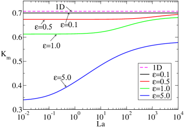
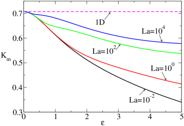
Figure 7: Wavenumber at the maximum growth rate, $K_{m}$, as a function of: (a) $La$ for different $\varepsilon$’s, and (b) $\varepsilon$ for different $La$’s. The solid lines corresponds to 2D model, and the dashed line to the 1D (long wave) model, $K_{m}^{1D}=1/\sqrt{2}=0.707$.

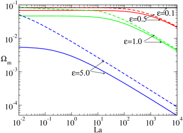
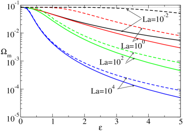
Figure 8: Maximum growth rates, $\Omega_{m}$, as a function of: (a) $La$ for different $\varepsilon$’s, and (b) $\varepsilon$ for different $La$’s. The solid lines corresponds to 2D model, and the dashed line to the 1D (long wave) model (same colour implies same $\varepsilon$ in (a), and same $La$ in (b)). The upper dotted line in both figures is the purely viscous ($La=0$) growth rate, $\Omega_{m,vis}=1/12=0.0833$. In (a), the 1D and 2D models for $\varepsilon=0.1$ are graphically superimposed to the this value of $\Omega_{m}$.

6 Numerical simulations

In order to analyse the validity range of the predictions of both LSA’s described above, we perform numerical simulations of the instability by solving the complete set of Navier-Stokes equations. Here, we use the two-phase flow, moving mesh interface of COMSOL Multiphysics. It solves the full incompressible Navier–Stokes equations using the Finite Element technique in a domain which deforms with the moving fluid interface by using the Arbitrary Lagrangian-Eulerian (ALE) formulation. The interface displacement is smoothly propagated throughout the domain mesh using the Winslow smoothing algorithm. The main advantage of this technique compared to others such as the Level Set of Phase Field techniques is that the fluid interface is and remains sharp. The main drawback, on the other hand, is that the mesh connectivity must remain the same, which precludes the modelling of situations for which the topology might change. The default mesh used throughout is unstructured and has $2940$ triangular elements (P1 linear elements for both velocity and pressure). Automatic remeshing is enabled to allow the solution to proceed even for large domain deformation when the mesh becomes severely distorted. The mesh nodes are constrained to the plane of the boundary they belong to for all but the free surface.

We adapt the same physical boundary conditions used above to the complete (nonlinear) 2D problem. Thus, we write the kinematic condition as:

$$\left({\bf v}-\frac{\partial h}{\partial t}\right)\cdot\bf n=0,$$ (70)

$\bf n$ being the external unit normal vector. Both surface tension and disjoining pressure exert normal stresses at the liquid-air interface

$${\cal S}\cdot{\bf n}=\left(\sigma{\cal C}-\kappa f(h)\right){\bf n},$$ (71)

where ${\cal C}=-{\nabla}_{s}\cdot{\bf n}$ is the curvature of the free surface, $\nabla_{s}=\bf I_{s}\cdot\nabla$ is the surface gradient operator, and ${\bf I}_{s}={\bf I}-{\bf n\,n}$ the surface identity tensor. At the ends of the domain ($x=0$ and $x=d$) periodic boundary conditions are applied for both the velocity field and shape of the free surface. On the liquid–solid interface, the the no-slip and no-penetration conditions ($\bf v=0$) are applied.

Since we must have the same length scale in both $x$ and $z$ directions in the solution of the full non-linear N–S equations, we define now a slightly different dimensionless set of units than in LSA for the long wave approximation (see Eq. (25)). Thus, the dimensionless variables in the numerical simulations are given by:

$$z=\ell\tilde{z},\quad x=\ell\tilde{x},\quad t=\tau\tilde{t},\quad u=\frac{\gamma}{\mu}\tilde{u},\quad w=\frac{\gamma}{\mu}\tilde{w},\quad p=\frac{\gamma}{\ell}\tilde{p},$$ (72)

which yields the dimensionless form of Navier–Stokes equations

$$La\left(\frac{\partial\tilde{u}}{\partial\tilde{t}}+\tilde{u}\frac{\partial\tilde{u}}{\partial\tilde{x}}+w\frac{\partial\tilde{u}}{\partial\tilde{z}}\right) = -\frac{\partial\tilde{p}}{\partial\tilde{x}}+\left(\frac{\partial^{2}\tilde{u}}{\partial{\tilde{x}}^{2}}+\frac{\partial^{2}\tilde{u}}{\partial{\tilde{z}}^{2}}\right),$$ (73)

$$La\left(\frac{\partial\tilde{w}}{\partial\tilde{t}}+\tilde{u}\frac{\partial\tilde{w}}{\partial\tilde{x}}+\tilde{w}\frac{\partial\tilde{w}}{\partial\tilde{z}}\right) = -\frac{\partial\tilde{p}}{\partial\tilde{z}}+\left(\frac{\partial^{2}\tilde{w}}{\partial{\tilde{x}}^{2}}+\frac{\partial^{2}\tilde{w}}{\partial{\tilde{z}}^{2}}\right).$$ (74)

In particular, the boundary condition at the free surface, Eq. (71), becomes

$$\tilde{\cal S}\cdot{\bf n}=\left(\tilde{\cal C}-\frac{\varepsilon}{g_{0}}f(\tilde{h})\right){\bf n}.$$ (75)

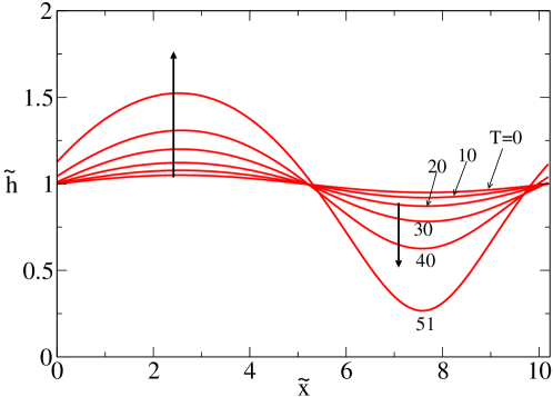
Figure 9: Time evolution of thickness profile for $La=1$ and $\varepsilon=1$. We use $A_{0}=0.05$.

In order to observe the evolution of the mode with maximum growth rate of the 2D model, we choose the length of the domain size in $x$-direction as $\tilde{d}=\tilde{\lambda}_{m}=2\pi/K_{m}^{2D}$. Note that this value is not coincident with $K_{m}^{1D}$ (see Fig. 7). Thus, we use the following monochromatic initial perturbation of the free surface

$$\tilde{h}(x,t=0)=\varepsilon+A_{0}\sin\left(\frac{2\pi\tilde{x}}{\tilde{d}}\right),$$ (76)

where $A_{0}$ is a small amplitude ($A_{0}=0.05$ in the present calculations). In Fig. 9 we show a time evolution of the thickness profile for $La=1$ and $\varepsilon=1$ (we use $(n,m)=(3,2)$ and $\tilde{h}_{\ast}=10^{-2}$ in all the following cases, unless otherwise stated). We carry on the simulation until the film becomes too close to $\tilde{h}_{\ast}$, where the numerical method is unable to converge, although continuation is sometimes possible by using automatic remeshing.

We study the evolution of the instability by tracking the maximum and minimum amplitudes of the free surface deformation by defining

$$A_{max}(\tilde{t}) = \max_{0\leq\tilde{x}\leq\tilde{L}}\left|1-\frac{\tilde{h}(\tilde{t})}{\epsilon}\right|,$$ (77)

$$A_{min}(\tilde{t}) = \min_{0\leq\tilde{x}\leq\tilde{L}}\left|1-\frac{\tilde{h}(\tilde{t})}{\epsilon}\right|.$$ (78)

These results are plotted in Fig. 10 for the same values of $La$ used in Fig. 6, but $\varepsilon=0.5,1,2$. The numerical non-linear solution of the problem shows that both $A_{max}$ and $A_{min}$ are practically coincident during a relatively long time of the evolution. Within the wide ranges of $La$ and $\varepsilon$ shown in Fig. 10, this behavior is observed for at least two thirds of the total time required for the full development of the instability. This indicates that a linear models, like those presented previously, are relevant to describe the flow beyond the onset of the instability.

In order to compare the numerical results with the linear models, we plot in Fig. 10 the expected exponential behavior as,

$$A=0.05\,e^{\alpha(T-T_{0})}$$ (79)

where $\alpha$ is given by the predicted growth rate for $K_{m}^{2D}$, and $T_{0}$ stands for a possible time shifting. For 1D model, $\alpha$ is the corresponding growth rate for $K_{m}^{2D}$, i.e. $\alpha=\Omega^{1D}(K_{m}^{2D})$, which in general does not coincide with the maximum growth rate within this approximation. For 2D model, $\alpha=\Omega^{2D}(K_{m}^{2D})=\Omega_{m}$, which is indeed the absolute maximum for this approach. Moreover, after separation of $A_{max}$ and $A_{min}$, we expect that $A_{max}$ remains closer to the exponential growth than $A_{min}$, which is more strongly affected by the presence of the substrate. This effect is certainly observed in the numerical results.

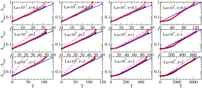
Figure 10: Time lines of the amplitudes $A_{max}$ ($\circ$) and $A_{min}$ ($\vartriangle$) with $T={\tilde{t}}\varepsilon^{3}$ for different values of $La$ and $\varepsilon$. The lines correspond to the exponential behavior $A=0.05\,\exp[\Omega_{m}(T-T_{0})]$, where $\Omega_{m}$ corresponds to the value given by either the 2D (solid line) or 1D (dashed line) model. $T_{0}=0$ except for the cases $(La,\varepsilon)=(10^{4},0.5)$, $(10^{2},1)$ and $(10^{4},1)$.

Figure 10 shows that for small $La$, say $La=0.01$ and $1$, there is a very good agreement with the exponential behavior of the 2D model prediction (solid blue lines). In general, the 1D model is not a good approximation, except for very small $\varepsilon$, as expected. For both models, we use $T_{0}=0$ since the behavior of $A_{max}$ and $A_{min}$ is of the exponential type from the very beginning. This type of growth is also observed for $La=100$ and $\varepsilon=0.5$, but $T_{0}\neq 0$ is needed for large $\varepsilon$, thus indicating the presence of a very early stage with slower (non exponential) growth. This effect is still more pronounced for $La$ as large as $La=10^{4}$. In these cases, where there is still an acceptable agreement between the 2D model and the numerics for relatively large $\varepsilon$. However, for this very large value of $La$, as $\varepsilon$ is decreased neither 1D nor 2D models are able to capture the actual evolution of the complete nonlinear problem. This issue deserves further investigation, which is out of the scope of the present paper and remains for future work.

It is worth noting that the exponents $n$ and $m$ of the disjoining pressure in Eq. (3) do not a play a role in both linear analyses performed here. Their influence in this stage is somehow hidden in the length scale, $\ell$, defined in Eq. (20). However, some effects are expected in the numerical solution of the fully nonlinear N–S equations, since they appear in the boundary condition given by Eq. (75). Figure 11a shows a comparison of the time evolution of $A_{max}$ and $A_{min}$ for $(n,m)=(3,2)$ and $(9,3)$, which are typical pairs of exponents used in the literature (Schwartz, 1998). Clearly, both cases are practically coincident in the linear stage, and are in agreement with the linear 2D model. For larger times, the corresponding non-linear regimes strongly differ, thus leading to different breakup times, so that the effect of the exponents is limited to the short final non-linear stage. Similarly, Fig. 11b shows the same time lines for two different values of $\tilde{h}_{\ast}$ and a given pair of $(n,m)$. Also in this case, only the nonlinear stage of the evolution changes for different thicknesses $\tilde{h}_{\ast}$, without any significant change of the early linear stage. For $\tilde{h}_{\ast}$ as small as $\tilde{h}_{\ast}=10^{-3}$, no difference is observed neither in the linear nor in the nonlinear stages. This so because $\tilde{h}_{\ast}$ becomes negligible with respect to $\tilde{h}_{0}$.

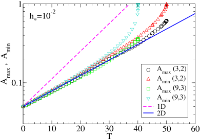
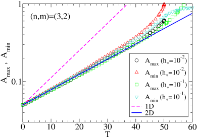
Figure 11: Time lines of the amplitudes $A_{max}$ and $A_{min}$ for $La=1$ and $\varepsilon=1$ for: (a) two different pairs of exponents $(n,m)$, (b) two different values of $\tilde{h}_{\ast}$. Symbols indicate numerical simulations, lines the predictions of linear models.

7 Summary and conclusions

In this work, we have developed three different approaches to study the instability of a flat liquid thin film under partial wetting conditions, and subject to intermolecular forces (disjoining pressure): long wave 1D model (with inertia), liner 2D model, and fully nonlinear numerical simulations. Firstly, we have extended the purely viscous analysis within the lubrication approximation to one where inertial effects are taken into account, which we call for brevity 1D model. The LSA of this model shows that inertia does not lead to new regions of instability compared with the purely viscous case. Instead, it adds new stable modes: some which are exponentially decaying, and others which are damped oscillations. The former extend over the same range of the unstable modes and even beyond, while the latter appear for larger wavenumbers. In the unstable region of most interest here, we find that both the marginal wavenumber and that of the maximum growth rate do not change at all with the addition of inertia. However, the results clearly show that the growth rates of the instability decrease as inertial effects are stronger. The intensity of these effects is here quantified by a single parameter, namely the modified Laplace number, $La^{\ast}=La\,\varepsilon^{5}$. Therefore, the approximation can be applied only for large $La$, since $\varepsilon\ll 1$ is required for the approach to be valid.

Secondly, we develop a LSA of the Navier–Stokes equation, so that the restriction of small aspect ratio, $\varepsilon$, is no longer required. This calculation, called for brevity 2D model, is particularly useful to assess the accuracy of the 1D model predictions. The main difference between these models is the way that inertia is treated. In linear 1D model, the convective terms for the horizontal direction are still taken into account, while horizontal and vertical convective terms are neglected in the linear 2D model, but the viscous Laplacian term is now fully conserved for both directions. Thus, we have now two independent parameters to characterize the flow, namely $La$ and $\varepsilon$. The 2D model shows that the marginal wavenumber remains the same as 1D model, and does not depend on $La$. However, unlike 1D model, 2D model shows that $K_{m}$ is not constant, and decreases as $La$ increases. This is an important result, since it shows that inertia can modify the distance between the final drops, which must be more separated with respect to the purely viscous case.

With respect to the dependence of the growth rates with $La$, 2D model also shows that they decrease for increasing $La$, but the strength of the effect is greater than what is predicted by 1D model. Interestingly, the discrepancies between both models decrease as $La$ increases, i.e. for larger inertial effects. Note also that both models capture the main scaling of the dimensional growth rate, $\omega$, with the aspect ratio $\varepsilon$. Thus, we can write,

$$\omega_{1}(k)=\frac{\varepsilon^{3}}{\tau}\Omega_{1}(k\ell;La\,\varepsilon^{5}),\quad\omega_{2}(k)=\frac{\varepsilon^{3}}{\tau}\Omega_{2}(k\ell;La,\varepsilon)$$ (80)

where the subscripts $1$ and $2$ correspond to 1D and 2D models, respectively.

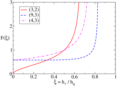
Figure 12: Function $F(\xi)$ that determines the influence of $h_{\ast}$ on the characteristic length scale, $\ell$.

Finally, we are concerned now with obtaining a prediction of the both $k_{m}$ and $\omega_{m}$ as a function of the film thickness, $h_{0}$, for a given experimental configuration. In order to do so, we recall that (Israelachvili, 1992)

$$\kappa=\frac{A}{6\pi h_{\ast}^{3}},$$ (81)

where $A$ is the Hamaker constant. Thus, the characteristic length, $\ell$, given by Eq. (20) can be written as

$$\ell=F(\xi)\frac{h_{0}^{2}}{L},$$ (82)

where

$$L=\sqrt{\frac{A}{6\pi\gamma}},\qquad F(\xi)=\sqrt{\frac{\xi^{3}}{g_{0}(\xi)}},$$ (83)

being $\xi=h_{\ast}/h_{0}$. The function $F(\xi)$, which describes the effects of $h_{\ast}$, is shown in Fig. 12 for three usual values of $(n,m)$. Interestingly, the cases with $m=3$ and large $n$ present a practically constant region for $\xi<0.5$, which is a typical range in experiments. In these cases, we notice that $\ell\propto h_{0}^{2}$, thus $\varepsilon\propto h_{0}^{-1}$ and $La\propto h_{0}^{2}$. Instead, if $m<3$, say $m=2$, the behaviour is different since $F\rightarrow 0$ for decreasing $h_{\ast}$. For $(3,2)$, we have $\ell\propto h_{0}^{3/2}$, thus $\varepsilon\propto h_{0}^{-1/2}$ and $La\propto h_{0}^{3/2}$.

These results shoud be taken into account when analyzing experimental data within a given hydrodynamic model. For instance, the lubrication approximation would not become more valid as $h_{0}$ decreases (as it could be expected a priori) since $\varepsilon$ increases for thinner films. In fact, let us consider the data from the experiments with melted copper films on a $SiO_{2}$ substrate reported in (González et al., 2013). In this case, we have $\gamma=1.304\,Kg/m^{3}$, $\mu=0.00438\,Pa\,s$, and the experiments could be fitted with a purely viscous lubrication model using $A=2.58~{}10^{-19}\,J$, $h_{\ast}=0.1\,nm$ and $(n,m)=(3,2)$. Thus, we calculate the corresponding values of $\varepsilon$ and $La$ for film thickness, $h_{0}$, in the interval $(1,100)\,nm$, as shown Fig. 13a. Note that even if inertial effects increase as $h_{0}$ increases, $\varepsilon$ decreases even faster, so that lubrication approximation assumptions apply for larger $h_{0}$’s (see also $La^{\ast}$ in Fig. 13b). Consistently, Fig. 13b indicates that the length $\ell$ (proportional to the critical wavelength) increases with $h_{0}$, so that wavelengths of some hundreds of nanometers should be expected for these film thicknesses.

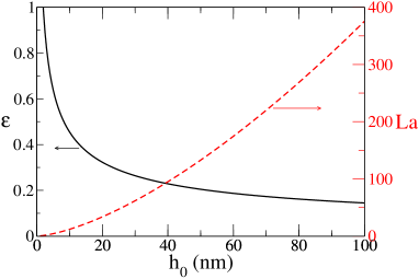
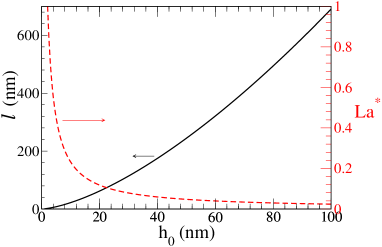
Figure 13: Dependence of the dimensionless parameters $\varepsilon$, $La$, $La^{\ast}$, and the characteristic length scale, $\ell$, as a function of the film thickness, $h_{0}$, for melted copper films

.

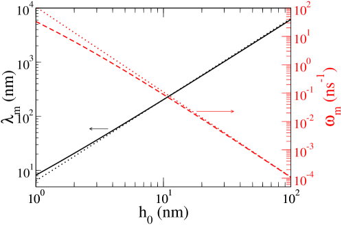
Figure 14: Wavelength of maximum growth rate, $\lambda_{m}$, and the corresponding growth, $\omega_{m}$, as a function of the film thickness, $h_{0}$, for melted copper films

In particular, we show the wavelength of maximum growth rate, $\lambda_{m}$, as well as the corresponding growth, $\omega_{m}$, as a function of $h_{0}$ in Fig. 14. The asymptotic power laws for large $h_{0}$, given by the lubrication approximation where $K_{m}=1/\sqrt{2}$ and $\Omega_{m}=1/12$ are (see also Eq. (25)),

$$\lambda_{m}=2\pi\sqrt{\frac{L^{2}}{h_{\ast}}}h_{0}^{3/2},\qquad\omega_{m}=\frac{\gamma}{3\mu}\frac{L^{4}}{h_{\ast}^{2}}h_{0}^{-3}.$$ (84)

These expressions are plotted as dotted lines in Fig. 14. Therefore, we conclude that both inertial and bidimensional effects are not significant if $h_{0}\gtrsim 20h_{\ast}$, being pretty safe to use lubrication approximation results to describe the instability even for large $La$ provided $h_{0}\gg h_{\ast}$, as in the experiments reported by González et al. (2013). However, for very thin nanometric films with $h_{0}\lesssim 10h_{\ast}$, these effects should be taken into account, specially when analyzing the growth rates of the unstable modes.

References

- Colinet et al. (2007) Colinet, P., H. Kaya, S. Rossomme, and B. Scheid (2007). Some advances in lubrication-type theories. Eur. Phys. J. Special Topics 146, 377–389.
- Craster and Matar (2009) Craster, R. V. and O. K. Matar (2009). Dynamics and stability of thin liquid films. Rev. Mod. Phys. 81, 1131.
- Diez and Kondic (2007) Diez, J. and L. Kondic (2007). On the breakup of fluid films of finite and infinite extent. Phys. Fluids 19, 072107.
- Eggers (1997) Eggers, J. (1997). Nonlinear dynamics and breakup of free-surface flows. Rev. Mod. Phy. 69, 865.
- González et al. (2013) González, A. G., J. A. Diez, Y. Wu, J. D. Fowlkes, P. D. Rack, and L. Kondic (2013). Instability of liquid Cu films on a SiO2 substrate. Langmuir 29, 9378–9387.
- Hocking and Davis (2002) Hocking, L. M. and S. H. Davis (2002). Inertial effects in time-dependent motion of thin films and drops. J. Fluid Mech. 467, 1–17.
- Israelachvili (1992) Israelachvili, J. N. (1992). Intermolecular and surface forces. New York: Academic Press. second edition.
- Kargupta et al. (2004) Kargupta, K., A. Sharma, and R. Khanna (2004). Instability, dynamics, and morphology of thin slipping films. Langmuir 20, 244.
- Lopez et al. (1997) Lopez, P. G., M. J. Miksis, and S. G. Bankoff (1997). Inertial effects on contact line instability in the coating of a dry inclined plane. Phys. Fluids 9, 2177.
- Nguyen et al. (2012) Nguyen, T. D., M. Fuentes-Cabrera, J. D. Fowlkes, J. A. Diez, A. G. González, L. Kondic, and P. D. Rack (2012). Competition between collapse and breakup in nanometer-sized thin rings using molecular dynamics and continuum modeling. Langmuir 28, 13960–13967.
- Oron et al. (1997) Oron, A., S. H. Davis, and S. G. Bankoff (1997). Long-scale evolution of thin liquid films. Rev. Modern Phys. 69, 931.
- Schwartz (1998) Schwartz, L. W. (1998). Hysteretic effects in droplet motions on heterogenous substrates: Direct numerical simulations. Langmuir 14, 3440.
- Schwartz and Eley (1998) Schwartz, L. W. and R. R. Eley (1998). Simulation of droplet motion of low-energy and heterogenous surfaces. J. Colloid Interface Sci. 202, 173.
- Thiele (2003) Thiele, U. (2003). Open questions and promising new fields in dewetting. Eur. Phys. J. E 12, 409.
- Thiele et al. (1998) Thiele, U., M. Mertig, and W. Pompe (1998). Dewetting of an evaporating thin liquid film: Heterogeneous nucleation and surface instability. Phys. Rev. Lett. 80, 2869–2872.
- Thiele et al. (2001) Thiele, U., M. G. Velarde, and K. Neuffer (2001). Dewetting: Film rupture by nucleation in the spinodal regime. Phys. Rev. Lett. 87, 016104.
- Ubal et al. (2014) Ubal, S., P. Grassia, D. M. Campana, M. D. Giavedoni, and F. A. Saita (2014). The influence of inertia and contact angle on the instability of partially wetting liquid strips: A numerical analysis study. Phys. Fluids 26, 032106.