High-order ADI schemes for convection-diffusion equations with mixed derivative terms

Abstract

We present new high-order Alternating Direction Implicit (ADI) schemes for the numerical solution of initial-boundary value problems for convection-diffusion equations with cross derivative terms. Our approach is based on the unconditionally stable ADI scheme proposed by Hundsdorfer Hund02 . Different numerical discretizations which lead to schemes which are fourth-order accurate in space and second-order accurate in time are discussed.

0.1 Introduction

We consider the multi-dimensional convection-diffusion equation

$$u_{t}=\mathrm{div}(D\nabla u)+c\cdot\nabla u$$ (1)

on a rectangular domain $\Omega\subset\mathbb{R}^{2}$, supplemented with initial and boundary conditions. In (1),

$$c=\left(\begin{array}[]{c}c_{1}\\ c_{2}\\ \end{array}\right),\quad D=\left(\begin{array}[]{cc}d_{11}&d_{12}\\ d_{21}&d_{22}\\ \end{array}\right),$$

are a given nonzero convection vector and a given, fully populated (non-diagonal), and positive definite diffusion matrix, respectively. Thus, both mixed derivative and convection terms are present in (1).

After rearranging, problem (1) may be formulated as

$$\frac{\partial u(x,y,t)}{\partial t}=\underbrace{(d_{12}+d_{21})\frac{\partial^{2}u}{\partial x\partial y}}_{=:F_{0}(u)}+\underbrace{(c_{1}\frac{\partial u}{\partial x}+d_{11}\frac{\partial^{2}u}{\partial x^{2}})}_{=:F_{1}(u)}+\underbrace{(c_{2}\frac{\partial u}{\partial y}+d_{22}\frac{\partial^{2}u}{\partial y^{2}})}_{=:F_{2}(u)}.$$ (2)

This type of convection-diffusion equations with mixed derivatives arise frequently in many applications, e.g. in financial mathematics for option pricing in stochastic volatility models or in numerical mathematics when coordinate transformations are applied. Such transformations are particularly useful to allow working on simple (rectangular) domains or on uniform grids (to have better accuracy). Thus, this approach allows to consider complex domains or to define non-uniform meshes to take into account the stiffness behavior of the solution in some part of the domain.

In the mathematical literature, there exist a number of numerical approaches to approximate solutions to (1), e.g. finite difference schemes, spectral methods, finite volume and finite element methods. Here, we consider (1) on a rectangular domain $\Omega\subset\mathbb{R}^{2}$. In this situation a finite difference approach seems most straight-forward.

The Alternating Direction Implicit (ADI) method introduced by Peaceman and Rachford PeacmanRachford95 , Douglas Douglas ; Gunn , Fairweather and Mitchell Fairweather is a very powerful method that is especially useful for solving parabolic equations on rectangular domains. Beam and Warming BeamWarming , however, have shown that no simple ADI scheme involving only discrete solutions at time levels $n$ and $n+1$ can be second-order accurate in time in the presence of mixed derivatives ($F_{0}\neq 0$ in (2)). To overcome this limitation and construct an unconditionally stable ADI scheme of second order in time, a number of results have been given by Hundsdorfer Hund02 ; Verwer and more recently by in ’t Hout and Welfert HoutWelfert07 . These schemes are second-order accurate in time and space.

High-Order Compact (HOC) schemes (see, e.g. Gupta ; Rigal99 ) employ a nine-point computational stencil using the eight neighbouring points of the reference grid point only and show good numerical properties. Several papers consider the application of HOC schemes (fourth order accurate in space) for two-dimensional convection-diffusion problems with mixed derivatives FournieKaraa06 ; DuringFournie12 but without ADI splitting. Moreover, the HOC approach introduces a high algebraic complexity in the derivation of the scheme.

We are interested in obtaining efficient, high-order ADI schemes, i.e. schemes which have a consistency order equal to two in time and to four in space, which are unconditionally stable and robust (no oscillations). We combine the second-order ADI splitting scheme presented in Hund02 ; HoutWelfert07 with different high-order schemes to approximate $F_{0},F_{1},F_{2}$ in (2). We note that some results on coupling HOC with ADI have been presented in KaraaZhang04 , however, without mixed derivative terms present in the equation.

Up to the knowledge of the authors there are currently no results for ADI-HOC in the presence of mixed derivative terms. In this preparatory work we validate the coupling of ADI and HOC by numerical experiments.

0.2 Splitting in time

In time, we consider the following splitting scheme presented in Hund02 ; HoutWelfert07 . We consider (2), and we look for a (semi-discrete) approximation $U^{n}\approx u(t_{n})$ with $t_{n}=n\Delta_{t}$ for a time step $\Delta_{t}$. The scheme used corresponds to

$$\left\{\begin{array}[]{l}Y^{0}=U^{n-1}+\Delta_{t}F(U^{n-1}),\\ Y^{1}=Y^{0}+\theta\Delta_{t}(F_{1}(Y^{1})-F_{1}(U^{n-1})),\\ Y^{2}=Y^{1}+\theta\Delta_{t}(F_{2}(Y^{2})-F_{2}(U^{n-1})),\\ \tilde{Y}^{0}=Y^{0}+\sigma\Delta_{t}(F(Y^{2})-F(U^{n-1})),\\ \tilde{Y}^{1}=\tilde{Y}^{0}+\theta\Delta_{t}(F_{1}(\tilde{Y}^{1})-F_{1}(Y^{2})),\\ \tilde{Y}^{2}=\tilde{Y}^{1}+\theta\Delta_{t}(F_{2}(\tilde{Y}^{2})-F_{2}(Y^{2})),\\ U^{n}=\tilde{Y}^{2},\end{array}\right.$$ (3)

with constant parameters $\theta$ and $\sigma,$ and $F=F_{0}+F_{1}+F_{2}.$ To ensure second-order consistency in time we choose $\sigma=1/2$. The parameter $\theta$ is arbitrary and typically fixed to $\theta=1/2$. The choice of $\theta$ is discussed in Hund02 . Larger $\theta$ gives stronger damping of implicit terms and lower values return better accuracy (some numerical results for $\theta=1/2+\sqrt{3}/6$ are given in section 0.4).

We note that $F_{0}$ is treated explicitly, whereas $F_{1},F_{2}$ (unidirectional contributions in $F$) are treated implicitly. In the following section, we discuss different high-order (fourth order) strategies for the discretization in space.

0.3 High-order approximation in space

For the discretization in space, we replace the rectangular domain $\Omega=[L_{1},R_{1}]\times[L_{2},R_{2}]\subset\mathbb{R}^{2}$ with $R_{1}>L_{1}$, $R_{2}>L_{2}$ by a uniform grid $Z=\{x_{i}\in\left[L_{1},R_{1}\right]:$ $x_{i}=L_{1}+(i-1)\Delta_{x}$, $i=1,\dots,N\}\times\{y_{j}\in\left[L_{2},R_{2}\right]:$ $y_{j}=L_{2}+(j-1)\Delta_{y}$, $j=1,\dots,M\}$ consisting of $N\times M$ grid points, with space steps $\Delta_{x}=(R_{1}-L_{1})/(N-1)$ and $\Delta_{y}=(R_{2}-L_{2})/(M-1)$. Let $u_{i,j}$ denote the approximate solution in $(x_{i},y_{j})$ at some fixed time (we omit the superscript $n$ to simplify the notation).

We present different fourth-order schemes to approximate $F_{0},F_{1},F_{2}$ in (3). The first one uses five nodes in each direction and the second one is compact. Both schemes are considered with boundary conditions of either periodic or Dirichlet type.

0.3.1 Fourth-order scheme using five nodes

We denote by $\delta_{x0}$, $\delta_{x+}$ and $\delta_{x-}$, the standard central, forward and backward finite difference operators, respectively. The second-order central difference operator is denoted by $\delta_{x}^{2}$,

$$\delta_{x}^{2}u_{i,j}=\delta_{x+}\delta_{x-}u_{i,j}=\frac{u_{i+1,j}-2u_{i,j}+u_{i-1,j}}{\Delta_{x}^{2}}.$$

The difference operators in the $y$-direction, $\delta_{y0}$, $\delta_{y+}$, $\delta_{y-}$ and $\delta_{y}^{2}$, are defined analogously. Then it is possible to define fourth-order approximations based on,

$$\left.\begin{array}[]{ll}\displaystyle(u_{x})_{i,j}&\displaystyle\approx\biggl{(}1-\frac{\Delta_{x}^{2}}{6}\delta_{x}^{2}\biggr{)}\delta_{x0}u_{i,j}=\frac{-u_{i+2,j}+8u_{i+1,j}-8u_{i-1,j}+u_{i-2,j}}{12\Delta_{x}},\\ \displaystyle(u_{y})_{i,j}&\displaystyle\approx\biggl{(}1-\frac{\Delta_{y}^{2}}{6}\delta_{y}^{2}\biggr{)}\delta_{y0}u_{i,j}=\frac{-u_{i,j+2}+8u_{i,j+1}-8u_{i,j-1}+u_{i,j-2}}{12\Delta_{y}},\\ \displaystyle(u_{xx})_{i,j}&\displaystyle\approx\biggl{(}1-\frac{\Delta_{x}^{2}}{12}\delta_{x}^{2}\biggr{)}\delta_{x}^{2}u_{i,j}=\frac{-u_{i+2,j}+16u_{i+1,j}-30u_{i,j}+16u_{i-1,j}-u_{i-2,j}}{12\Delta_{x}^{2}},\\ \displaystyle(u_{yy})_{i,j}&\displaystyle\approx\biggl{(}1-\frac{\Delta_{y}^{2}}{12}\delta_{y}^{2}\biggr{)}\delta_{y}^{2}u_{i,j}=\frac{-u_{i,j+2}+16u_{i,j+1}-30u_{i,j}+16u_{i,j-1}-u_{i,j-2}}{12\Delta_{y}^{2}},\\ \displaystyle(u_{xy})_{i,j}&\displaystyle\approx\biggl{(}1-\frac{\Delta_{x}^{2}}{6}\delta_{x}^{2}\biggr{)}\delta_{x0}\biggl{(}1-\frac{\Delta_{y}^{2}}{6}\delta_{y}^{2}\biggr{)}\delta_{y0}u_{i,j}\\ &\displaystyle=\frac{1}{144\Delta_{x}\Delta_{y}}\bigl{[}64(u_{i+1,j+1}-u_{i-1,j+1}+u_{i-1,j-1}-u_{i+1,j-1})\\ &\displaystyle\hskip 56.9055pt+8(-u_{i+2,j+1}-u_{i+1,j+2}+u_{i-1,j+1}+u_{i-2,j+1}\\ &\displaystyle\hskip 73.97733pt-u_{i-2,j-1}-u_{i-1,j-2}+u_{i+1,j-2}+u_{i+2,j-1})\\ &\displaystyle\hskip 56.9055pt+(u_{i+2,j+2}-u_{i-2,j+2}+u_{i-2,j-2}-u_{i+2,j-2})\bigr{]}.\end{array}\right.$$ (4)

For each differential operators appearing in $F_{0}$, $F_{1}$ and $F_{2}$, we use these five-points fourth-order difference formulae.

Combining this spatial discretization with the time splitting (3), we obtain a high-order, five-points ADI scheme denoted HO5. Its order of consistency is two in time and four in space.

0.3.2 Fourth-order compact scheme

We start by deriving a fourth-order HOC scheme for

$$F_{1}(u)=d_{11}\frac{\partial^{2}u}{\partial x^{2}}+c_{1}\frac{\partial u}{\partial x}=g,$$ (5)

with some arbitrary right hand side $g.$ We employ central difference operators to approximate the derivatives in (5) using

$$\frac{\partial u}{\partial x}(x_{i},y_{j}) =\delta_{x0}u_{i,j}-\frac{\Delta_{x}^{2}}{6}{\frac{\partial^{3}u}{\partial x^{3}}(x_{i},y_{j})}+\mathcal{O}(\Delta_{x}^{4}),$$ (6)

$$\frac{\partial^{2}u}{\partial x^{2}}(x_{i},y_{j}) =\delta_{x}^{2}u_{i,j}-\frac{\Delta_{x}^{2}}{12}{\frac{\partial^{4}u}{\partial x^{4}}(x_{i},y_{j})}+\mathcal{O}(\Delta_{x}^{4}).$$ (7)

By differentiating (5), we can compute the following auxiliary relations for the derivatives appearing in (6), (7) (in the following, for the sake of brevity we omit the argument $(x_{i},y_{j})$ of the continuous functions)

$$\frac{\partial^{3}u}{\partial x^{3}} =\frac{1}{d_{11}}\frac{\partial g}{\partial x}-\frac{c_{1}}{d_{11}}\frac{\partial^{2}u}{\partial x^{2}},$$ (8)

$$\frac{\partial^{4}u}{\partial x^{4}} =\frac{1}{d_{11}}\frac{\partial^{2}g}{\partial x^{2}}-\frac{c_{1}}{d_{11}}{\frac{\partial^{3}u}{\partial x^{3}}}=\frac{1}{d_{11}}\frac{\partial^{2}g}{\partial x^{2}}-\frac{c_{1}}{d_{11}}\left(\frac{1}{d_{11}}\frac{\partial g}{\partial x}-\frac{c_{1}}{d_{11}}\frac{\partial^{2}u}{\partial x^{2}}\right).$$ (9)

Hence, using (8) and (9) in (6) and (7), respectively, equation (5) can be approximated by

$$d_{11}\delta_{x}^{2}u_{i,j}+c_{1}\delta_{x0}u_{i,j}=g_{i,j}+\frac{\Delta_{x}^{2}}{12}\left(\frac{c_{1}}{d_{11}}\frac{\partial g}{\partial x}+\frac{\partial^{2}g}{\partial x^{2}}-\frac{c_{1}^{2}}{d_{11}}\frac{\partial^{2}u}{\partial x^{2}}\right)+\mathcal{O}(\Delta_{x}^{4}).$$ (10)

We note that all derivatives on the right hand side of (10) can be approximated on a compact stencil using second-order central difference operators. This yields a high-order compact scheme of fourth order for (5) which is given by

$$d_{11}\delta_{x}^{2}u_{i,j}+c_{1}\delta_{x0}u_{i,j}+\frac{\Delta_{x}^{2}}{12}\frac{c_{1}^{2}}{d_{11}}\delta_{x}^{2}u_{i,j}=g_{i,j}+\frac{\Delta_{x}^{2}}{12}\left(\frac{c_{1}}{d_{11}}\delta_{x0}g_{i,j}+\delta_{x}^{2}g_{i,j}\right).$$ (11)

In a similar fashion we can discretize the operator $F_{2}(u)=g$ by a high-order compact scheme of fourth order given by

$$d_{22}\delta_{y}^{2}u_{i,j}+c_{2}\delta_{y0}u_{i,j}+\frac{\Delta_{y}^{2}}{12}\frac{c_{2}^{2}}{d_{22}}\delta_{y}^{2}u_{i,j}=g_{i,j}+\frac{\Delta_{y}^{2}}{12}\left(\frac{c_{2}}{d_{22}}\delta_{y0}g_{i,j}+\delta_{y}^{2}g_{i,j}\right).$$ (12)

Defining vectors $U=(u_{1,1},\dots,u_{N,M})$ and $G=(g_{1,1},\dots,g_{N,M})$, we can state these schemes (11) and (12) in matrix form $A_{x}U=B_{x}G$ (for $F_{1}(u)=g$) and $A_{y}U=B_{y}G$ (for $F_{2}(u)=g$), respectively. We apply these HOC schemes to find the unidirectional contributions $Y^{1}$, $\tilde{Y^{1}}$, and $Y^{2}$, $\tilde{Y^{2}}$ in (3), respectively. For example, to compute

$$Y^{1}=Y^{0}+\frac{\Delta_{t}}{2}(F_{1}(Y^{1})-F_{1}(U^{n-1}))$$

in the second step of (3) (which is equivalent to $F_{1}(Y^{1}-U^{n-1})=-\frac{2}{\Delta_{t}}(Y^{0}-Y^{1})$), we use $A_{x}(Y^{1}-U^{n-1})=B_{x}(-\frac{2}{\Delta_{t}}(Y^{0}-Y^{1}))$ that can be rewrite into

$$\left(B_{x}-\frac{\Delta_{t}}{2}A_{x}\right)Y^{1}=B_{x}Y^{0}-\frac{\Delta_{t}}{2}A_{x}U^{n-1}.$$

Note that the matrix $(B_{x}-(\Delta_{t}/2)\,A_{x})$ appears twice in (3), in steps two and five. Similarly, $(B_{y}-(\Delta_{t}/2)\,A_{y})$ appears in steps three and six of (3). Hence, using LU-factorisation, only two matrix inversions are necessary in each time step of (3). Moreover, for the case of constant coefficients, these matrices can be LU-factorized before iterating in time to obtain an even more efficient algorithm.

To compute $Y^{0}$ and $\tilde{Y^{0}}$ in steps one and four of (3) which require evaluation of $F_{0}$ (mixed term) we use an explicit approximation using the five-points fourth-order formulae (4).

Combining this spatial discretization with the time splitting (3), we obtain a high-order compact ADI scheme denoted HOC. Its order of consistency is two in time and four in space.

0.4 Numerical experiments

We present numerical experiments on a square domain $\Omega=[0,1]\times[0,1]$ for two types of boundary conditions, periodic and Dirichlet type. The initial condition is given at time $T_{0}=0$ and the solution is computed at the final time $T_{f}=0.1$ with different meshes $\Delta_{x}=\Delta_{y}=h$ and different time steps $\Delta_{t}$. In our numerical tests we focus on the errors with respect to time and to space.

In the first part, we consider the periodic boundary value problem considered in HoutWelfert07 . We implement the scheme detailed in HoutWelfert07 based on second-order finite difference approximations (referred to as CDS below) and compare its behaviour to our new schemes HO5 (section 0.3.1) and HOC (section 0.3.2). In the second part, we consider Dirichlet boundary conditions and restrict our study to the more interesting HOC scheme. In that part, we extend the splitting scheme to a convection-diffusion equation with source term.

0.4.1 Periodic boundary conditions

The problem given in HoutWelfert07 is formulated on the domain $\Omega=[0,1]\times[0,1]$. The solution $u$ satisfies (1) where

$$c=-\left(\begin{array}[]{c}2\\ 3\\ \end{array}\right),\quad D=0.025\left(\begin{array}[]{cc}1&2\\ 2&4\\ \end{array}\right),$$

with periodic boundary conditions and initial condition $u(x,y,T_{0})=e^{-4(\sin^{2}(\pi x)+\cos^{2}(\pi y))}$. We employ the splitting (3) with $\sigma=1/2$ and $\theta=1/2$.

We first present a numerical study to compute the order of convergence in time of the schemes CDS, HO5 and HOC. Asymptotically, we expect the error $\epsilon$ to converge as

$$\epsilon=C\Delta_{t}^{m}$$

at some rate $m$ with $C$ representing a constant. This implies

$$\log(\epsilon)=\log(C)+m\log(\Delta_{t}).$$

Hence, the double-logarithmic plot $\epsilon$ against $\Delta_{t}$ should be asymptotic to a straight line with slope $m$ that corresponds to the order of convergence in time of the scheme. We denote by $\epsilon_{2}$ and $\epsilon_{\infty}$ the errors in the $l_{2}$-norm and $l_{\infty}$-norm, respectively. We refer to Table 0.4.1 for the order of convergence in time computed for different fixed mesh widths $h\in\{0.1,0.0.025,0.00625\}$ and time steps $\Delta_{t}\in[T_{f}/30,T_{f}/90]$. The solution computed for $\Delta_{t}=T_{f}/100$ is considered as reference solution to compute the errors. The global errors for the splitting behave like $C(\Delta_{t})^{2}$. We also observe that the constant $C$ only depends weakly on the spatial mesh widths $h$.

Table 1: Numerical convergence rates in time for $\theta=\frac{1}{2}$

Scheme	$l_{2}$-error convergence rate		$l_{\infty}$-error convergence rate
	$h=0.1$   $h=0.025$   $h=0.00625$		$h=0.1$   $h=0.025$   $h=0.00625$
CDS	2.2002     2.1975       2.1969		2.1973     2.1958       2.1956
HO5	2.1999     2.1973       2.1969		2.1992     2.1953       2.1955
HOC	2.2002     2.1973       2.1969		2.2007     2.1953       2.1955

In the following, we study the spatial convergence. The double-logarithmic plots $\epsilon_{2}$ and $\epsilon_{\infty}$ against $h$ give the rates of convergence. Contrary to the time convergence, the order now depends on the parabolic mesh ratio $\mu=\Delta_{t}/\Delta_{x}^{2}$, so the numerical tests are performed for a set of different constant values of $\mu$. For simulations, $\mu$ is fixed at constant values $\mu\in\{0.4,0.2,0.1,0.005\}$ while $\Delta_{x}=\Delta_{y}=h\to 0$ ($\Delta_{t}$ is then given by $\Delta_{t}=\mu h^{2}$). The results for the $l_{2}$-error are given in Table 0.4.1 and for the $l_{\infty}$-error in Table 0.4.1. The solution computed for $h=0.00625$ is used as reference solution to compute the errors.

Table 2: Numerical convergence rates in space of $l_{2}$-error for fixed $\mu$ as $\Delta_{x},\,\Delta_{t}\to 0$ and $\theta=\frac{1}{2}$

Scheme	$\mu=0.4$	$\mu=0.2$	$\mu=0.1$	$\mu=0.05$
CDS	1.7828	1.7909	1.7821	1.7845
HO5	2.2291	2.5188	2.8153	3.0672
HOC	2.2685	2.5191	2.8152	3.0671

Table 3: Numerical convergence rates in space of $l_{\infty}$-error for fixed $\mu$ as $\Delta_{x},\,\Delta_{t}\to 0$ and $\theta=\frac{1}{2}$

Scheme	$\mu=0.4$	$\mu=0.2$	$\mu=0.1$	$\mu=0.05$
CDS	1.7170	1.7125	1.7040	1.7038
HO5	2.2931	2.6166	2.9182	3.1584
HOC	2.3175	2.6176	2.9184	3.1584

Remark: The choice of the parameter $\theta$ is discussed in Hund02 . However, for the convergence rates, $\theta$ seems to have little influence. For example, for the scheme HO5 with $\theta={1}/{2}+\sqrt{3}/{6}$ we obtain very similar results as shown in Table 0.4.1.

Table 4: Numerical convergence rates in space for HO5 for fixed $\mu$ as $\Delta_{x},\,\Delta_{t}\to 0$ and $\theta=\frac{1}{2}+\frac{\sqrt{3}}{6}$

	$\mu=0.4$	$\mu=0.2$	$\mu=0.1$	$\mu=0.05$
$l_{2}$ rate	2.2310	2.5186	2.8152	3.0671
$l_{\infty}$ rate	2.2938	2.6164	2.9181	3.1584

0.4.2 Dirichlet Boundary conditions

In this section we only consider the HOC scheme which presents more interesting properties than the other schemes. Indeed, compared to CDS, its accuracy is larger and compared to HO5, no specific treatment at the boundaries is required for the uni-directional terms $F_{1}$, $F_{2}$, the compact scheme is optimal in this respect. A particular treatment is necessary when ghost points appear in the explicit approximation of the mixed term $F_{0}$. To preserve the global performance, the accuracy of the approximation near the boundary conditions has to be sufficiently high. We have used a sixth-order approximation in one direction (although lower order may also be used GusBC ). For example, for $u_{0,j}$ on the boundary, at a ghost point $u_{-1,j}$ we impose u_-1,j= 5 u_0,j -10 u_1,j+ 10 u_2,j -5 u_3,j+u_4,j.

For the numerical tests, we consider the problem u_t = div (D∇u) + c ⋅∇u+ S on the domain $\Omega=[0,1]\times[0,1]$ where c=-( 23 ),  D= 0.025 ( 1224 ), and the source term $S$ is determined in such a way that the solution is equal to $u(x,y,t)=-\frac{1}{t+1}\sin(\pi x)\sin(\pi y).$ The Dirichlet boundary condition and initial condition are deduced from the solution. To incorporate the source term $S$ in the splitting (3), $F$ needs to be replaced by $F+S$. More specifically, $F(U^{n-1})$ is replaced by $F(U^{n-1})+S(t^{n-1})$ and $F(Y^{2})$ by $F(Y^{2})+S(t^{n})$. We perform the same numerical experiments as in the previous section. The final time is fixed to $T_{f}=0.1$ and the errors are computed with respect to a reference solution computed on a fine grid in space ($\Delta_{x}=\Delta_{y}=0.00625$). Different meshes in space are considered for $\Delta_{x}=\Delta_{y}=h$ and $h\in\{0.1,0.05,0.025,0.0125\}$. For $\mu=0.4$ the double-logarithmic plots $\epsilon_{2}$ and $\epsilon_{\infty}$ against $h$ are given in Figure 1.

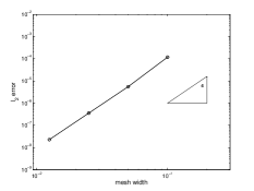
Figure 1: Numerical convergence rate in space for HOC ($\theta=\frac{1}{2}$) and $\mu=0.4$.

The results of several numerical tests are reported in Table 0.4.2 for fixed parabolic mesh ratio $\mu=\Delta_{t}/\Delta_{x}^{2}$ while $\Delta_{x},\,\Delta_{t}\to 0$. In all situations, the new HOC scheme shows a good performance with fourth-order convergence rates in space, independent of the parabolic mesh ratio $\mu$.

Table 5: Numerical convergence rates of $l_{2}$-error and $l_{\infty}$-error for HOC ($\theta=\frac{1}{2}$) for different constant values of $\mu$ (Dirichlet boundary conditions).

	$\mu=0.4$	$\mu=0.2$	$\mu=0.1$	$\mu=0.05$
$l_{2}$ rate	4.0971	4.1875	4.2129	4.2196
$l_{\infty}$ rate	4.1530	4.2372	4.2717	4.2806

0.5 Conclusion

We have presented new high-order Alternating Direction Implicit (ADI) schemes for the numerical solution of initial-boundary value problems for convection-diffusion equations with mixed derivative terms. Using the unconditionally stable ADI scheme from Hund02 we have proposed different spatial discretizations which lead to schemes which are fourth-order accurate in space and second-order accurate in time.

We have performed a numerical convergence analysis with periodic and Dirichlet boundary conditions where high-order convergence is observed. In some cases, the order depends on the parabolic mesh ratio. More detailed discussions of these schemes including this dependence and a stability analysis will be presented in a forthcoming paper.

References

- (1) D.W. Peaceman and H.H. Rachford Jr., The numerical solution of parabolic and elliptic differential equations, J. Soc. Ind. Appl. Math., 3, 28–41, (1959).
- (2) R.M. Beam and R.F. Warming, Alternating Direction Implicit methods for parabolic equations with a mixed derivative, Siam J. Sci. Stat. Comput., 1(1), (1980).
- (3) M. Fournié and S. Karaa, Iterative methods and high-order difference schemes for 2D elliptic problems with mixed derivative, J. Appl. Math. Computing, 22 (3), 349–363, (2006).
- (4) J. Douglas, Alternating direction methods for three space variables, Numer. Math., 4, 41–63, (1962).
- (5) J. Douglas and J. E. Gunn, A general formulation of alternating direction methods. I. Parabolic and hyperbolic problems, Numer. Math., 6, 428–453, (1964).
- (6) B. Düring and M. Fournié, High-order compact finite difference scheme for option pricing in stochastic volatility models. J. Comput. Appl. Math. 236(17), 4462–4473, (2012).
- (7) G. Fairweather and A. R. Mitchell, A new computational procedure for A.D.I. methods, SIAM J. Numer. Anal., 4, 163–170, (1967).
- (8) M.M. Gupta, R.P. Manohar and J.W. Stephenson, A single cell high-order scheme for the convection-diffusion equation with variable coefficients, Int. J. Numer. Methods Fluids, 4, 641–651, (1984).
- (9) B. Gustafsson, The convergence rate for difference approximation to general mixed initial-boundary value problems, SIAM J. Numer. Anal. 18(2), 179–190, (1981).
- (10) K.J. in ’t Hout and B.D. Welfert, Stability of ADI schemes applied to convection-diffusion equations with mixed derivative terms, Appl. Num. Math., 57, 19–35, (2007).
- (11) W. Hundsdorfer and J.G Verwer, Numerical solution of time-dependent advection-diffusion-reaction equations, Springer Series in Computational Mathematics, 33, Springer-Verlag, Berlin, (2003).
- (12) W. Hundsdorfer, Accuracy and stability of splitting with stabilizing corrections, Appl. Num. Math., 42, 213–233, (2002).
- (13) S. Karaa and J. Zhang, High-order ADI method for solving unsteady convection-diffusion problems, J. Comput. Phys., 198(1), 1–9, (2004).
- (14) A. Rigal, Schémas compacts d’ordre élevé: application aux problèmes bidimensionnels de diffusion-convection instationnaire I, C.R. Acad. Sci. Paris. Sr. I Math., 328, 535–538, (1999).