Constraining Big Bang lithium production with recent solar neutrino data

Abstract

The ³He($\alpha,\gamma$)⁷Be reaction affects not only the production of ⁷Li in Big Bang nucleosynthesis, but also the fluxes of ⁷Be and ⁸B neutrinos from the Sun. This double role is exploited here to constrain the former by the latter. A number of recent experiments on ³He($\alpha,\gamma$)⁷Be provide precise cross section data at $E$ = 0.5-1.0 MeV center-of-mass energy. However, there is a scarcity of precise data at Big Bang energies, 0.1-0.5 MeV, and below. This problem can be alleviated, based on precisely calibrated ⁷Be and ⁸B neutrino fluxes from the Sun that are now available, assuming the neutrino flavour oscillation framework to be correct. These fluxes and the standard solar model are used here to determine the ³He($\alpha,\gamma$)⁷Be astrophysical S-factor at the solar Gamow peak, $S_{34}^{\nu}(23^{+6}_{-5}\,\text{keV})$ = 0.548$\pm$0.054 keV b. This new data point is then included in a re-evaluation of the ³He($\alpha,\gamma$)⁷Be S-factor at Big Bang energies, following an approach recently developed for this reaction in the context of solar fusion studies. The re-evaluated S-factor curve is then used to re-determine the ³He($\alpha,\gamma$)⁷Be thermonuclear reaction rate at Big Bang energies. The predicted primordial lithium abundance is ${}^{7}{\rm Li/H}$ = 5.0 $\times 10^{-10}$, far higher than the Spite plateau.

I Introduction

The prediction of the light element abundances in Big Bang nucleosynthesis (BBN) is a pillar of modern cosmology. The consistent description of abundances over ten orders of magnitude can be considered as a big success. Latest data on the cosmic microwave background obtained by the Planck mission fix the baryon density and thus the baryon-photon ratio $\eta$ Planck Collaboration et al. (2014). However, there is still a puzzling disagreement between the observed abundance of ⁷Li in metal poor stars of ⁷Li/H = (1.6$\pm$0.3)$\times$10^-10 Olive and Particle Data Group (2014) and the prediction from BBN of ⁷Li/H = (4.95$\pm$0.39)$\times$10^-10 Coc et al. (2014). For a recent review of the lithium problem, see Ref. Fields (2011).

The production of ⁷Li in BBN depends on thermonuclear reaction rates $N_{\rm A}\langle\sigma v\rangle$, in particular that of the ³He($\alpha,\gamma$)⁷Be reaction called hereafter $R_{34}$. The thermonuclear reaction rate $R_{34}$, in turn, depends on the ³He($\alpha,\gamma$)⁷Be cross section $\sigma_{34}(E)$ and on the temperature $T$ prevalent in the astrophysical scenario under study:

$$R_{34}\equiv N_{\rm A}\langle\sigma v\rangle_{34}(T)=\\ N_{\rm A}\frac{(8/\pi)^{1/2}}{\mu^{1/2}(k_{\rm B}T)^{3/2}}\int\limits_{0}^{\infty}E\sigma_{34}(E)\exp\left(-\frac{E}{k_{\rm B}T}\right)dE$$ (1)

with $E$ the center-of-mass energy and $\mu=m_{3}m_{4}/(m_{3}+m_{4})$ the reduced mass of the two reaction partners ³He and ⁴He.

At astrophysical energies, the cross section $\sigma_{34}(E)$ exhibits an exponential-like energy dependence and can be parameterized as the astrophysical S-factor $S_{34}(E)$ which varies only very slowly with energy in the case of ³He($\alpha,\gamma$)⁷Be Adelberger et al. (2011). The S-factor is defined by the following equation:

$$\sigma_{34}(E)=\frac{1}{E}S_{34}(E)\exp\left[-2\pi Z_{1}Z_{2}\frac{e^{2}}{\hbar}\sqrt{\frac{\mu}{2E}}\right]$$ (2)

where $Z_{1}Z_{2}e^{2}$ is the product of the nuclear charges of the two reacting nuclei. Inserting Eq. (2) in Eq. (1), it follows:

$$R_{34}\propto\int\limits_{0}^{\infty}S_{34}(E)\exp\left[-\frac{E}{k_{\rm B}T}-2\pi Z_{1}Z_{2}\frac{e^{2}}{\hbar}\sqrt{\frac{\mu}{2E}}\right]dE$$ (3)

The exponential term is the so-called Gamow peak. The first term inside the exponential function forms the high-energy edge of the Gamow peak, given by the exponential decrease of the Maxwell-Boltzmann energy distribution. The second term forms the low-energy edge, given by the exponential-like decrease of the cross section. The energy range of this peak indicates where $S_{34}(E)$ must be integrated in order to obtain the thermonuclear reaction rate.

In the case of BBN, the S-factor must be known over a wide range in center-of-mass energies $E$. This range is estimated here by measuring the effect of a small change in the assumed S-factor at one given energy on the final ⁷Li abundance at the end of BBN, following the approach of Nollett and Burles Nollett and Burles (2000). The relevant energy range is found to be $E$ = 0.1-0.5 MeV (Fig. 1), consistent with the previous result by Ref. Nollett and Burles (2000). Subsequently, also the relevant temperature range for ⁷Be production in BBN is determined by arbitrarily setting $R_{34}$ to zero above a certain temperature, resulting in $T_{9}$=0.30-0.65, if a relevant effect is defined as a 2.5% contribution on the ⁷Be yield. When converting these temperatures to Gamow energies, the resultant relevant energy range is consistent with the one based on the Nollett and Burles Nollett and Burles (2000) approach, adopted here.

A number of recent $S_{34}(E)$ determinations are available at $E$ $>$ 0.3 MeV Nara Singh et al. (2004); Brown et al. (2007); di Leva et al. (2009); Carmona-Gallardo et al. (2012); Bordeanu et al. (2013); Kontos et al. (2013), allowing to form a weighted average and judge the precision of the recommended value (Fig. 1). However, this abundance of recent experimental data covers only the upper third of the relevant energy range. At lower energy, the exceedingly low cross section is a challenge for experimentalists. As a consequence, recent data for $E$ $\leq$ 0.3 MeV are available only from one experiment Bemmerer et al. (2006), performed at the LUNA accelerator deep underground in the Gran Sasso laboratory, Italy.

It should be noted that $S_{34}(E)$ data reported in the period from the 1950s to the 1980s Holmgren and Johnston (1959); Parker and Kavanagh (1963); Nagatani et al. (1969); Kräwinkel et al. (1982); Osborne et al. (1982); Alexander et al. (1984); Hilgemeier et al. (1988) are omitted from the present discussion, following the approach of a recent review Adelberger et al. (2011). These data Holmgren and Johnston (1959); Parker and Kavanagh (1963); Nagatani et al. (1969); Kräwinkel et al. (1982); Osborne et al. (1982); Alexander et al. (1984); Hilgemeier et al. (1988) are usually less well documented than the more recent works Nara Singh et al. (2004); Bemmerer et al. (2006); Brown et al. (2007); di Leva et al. (2009); Carmona-Gallardo et al. (2012); Bordeanu et al. (2013); Kontos et al. (2013) and have larger error bars.

The scarcity of recent low-energy $S_{34}(E)$ is addressed here based on the fact that actually the Gamow peak is rather narrow for low temperatures (see the solar Gamow peak in Fig. 1). Here, $S_{34}(E_{\rm Gamow}^{\rm Sun})$ is determined from $N_{\rm A}\langle\sigma v\rangle_{34}(T^{\rm Sun})$. The latest solar neutrino and cosmological data are used. The additional low-energy data point is used to re-determine the primordial lithium abundance.

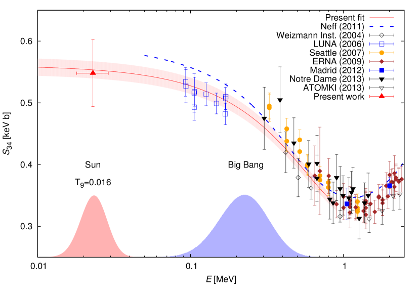
Figure 1: Cross section of the ³He($\alpha$,$\gamma$)⁷Be reaction, parameterized as the astrophysical $S$-factor. The present new data point (sec. V) is plotted together with previous experimental data Nara Singh et al. (2004); Bemmerer et al. (2006); Brown et al. (2007); di Leva et al. (2009); Carmona-Gallardo et al. (2012); Bordeanu et al. (2013); Kontos et al. (2013). The previous theoretical curve (dashed blue curve, Neff (2011)), and the present new extrapolation (red curve, shaded area for the uncertainty) are shown. The solar Gamow peak and the relevant energy range for BBN (see text) are displayed at the lower end of the plot.

A related idea has previously been explored by Cyburt et al. a decade ago Cyburt et al. (2004). That work was based on the neutrino data available at the time from the Sudbury Neutrino Observatory (SNO), and on the WMAP cosmological survey.

The present work uses newly available cross section, solar neutrino, microwave background, and neutron lifetime data, which are summarized in sec. II. Using an approach and errors described in sections III and IV, respectively, $S_{34}(E_{\rm Gamow}^{\rm Sun})$ is determined, limiting the use of the solar neutrino data to its strict range of applicability, the temperature range of the solar Gamow peak (sec. V.1). Subsequently, the new data point is included in a re-evaluation of the ³He($\alpha$,$\gamma$)⁷Be S-factor at Big Bang energies (sec. V.2). The predicted lithium abundance from BBN is subsequently updated (sec. VI), and a summary and outlook are given (sec. VII). In the appendix, the reaction rate is given both in parameterized and in tabular forms.

II Input data

The Sudbury Neutrino Observatory (SNO) reports a ⁸B solar neutrino flux of

$$\phi^{\text{exp}}_{\text{B}}=5.25\pm 0.16\text{ (stat)}^{+0.11}_{-0.13}\text{ (sys)}\times 10^{6}{\rm cm}^{-2}{\rm s}^{-1}$$

taking into account the loss in the amount of electron neutrinos due to the mixing among the neutrino families Aharmim et al. (2013). This is equivalent to 3.9% precision (systematical and statistical uncertainties combined in quadrature) and consistent with the determination made by Super-Kamiokande Smy (2013).

The flux of ⁷Be neutrinos was measured by BOREXINO Bellini et al. (2014), resulting in a value of

$$\phi^{\text{exp}}_{\text{Be}}=4.75^{+0.26}_{-0.22}\times 10^{9}{\rm cm}^{-2}{\rm s}^{-1}$$

with 5.5% total uncertainty.

The value for the baryonic density found by the Planck mission Planck Collaboration et al. (2014) is

$$\Omega_{b}h^{2}=0.02205\pm 0.00028$$

This parameter is an important input for BBN calculations, in addition to the thermonuclear reaction rates of the relevant nuclear reactions. The lifetime of the neutron has only a weak effect on Big Bang ⁷Li. For the present work, the recently recommended value of $\tau_{\rm n}=880.3\pm 1.1\text{ s}$ Olive and Particle Data Group (2014) is used for consistency. However, different values from 878-885 s change the final ⁷Li abundance only slightly.

III Description of the approach

In this work, no solar model calculations are performed. Instead, the so-called standard solar model developed by John Bahcall and co-workers is used, hereafter called SSM. The partial derivatives for the various SSM input parameters are available in tabulated form in the most recent SSM publication by Serenelli et al. Serenelli et al. (2013). Henceforth, the terminology and numbers from this work are used.

The SSM uses a number of input parameters, including the solar age, luminosity, opacity, diffusion rate, the key thermonuclear reaction rates (herein called $R_{i}$, where $i$ denotes the nuclear reaction under study), and the zero-age abundance of important elements (He, C, N, O, Ne, Mg, Si, S, Ar, Fe). A change in one or several of these input parameters may cause a change in the predicted neutrino fluxes. The sensitivity of flux $\phi_{i}$ for a variation in an arbitrary parameter $\beta_{j}$ can be expressed by the logarithmic partial derivatives $\alpha(i,j)$ given by the following relation:

$$\alpha(i,j)=\frac{\partial ln[\phi_{i}/\phi^{\rm SSM}_{i}]}{\partial ln[\beta_{j}/\beta^{\rm SSM}_{j}]}$$ (4)

where $\phi^{\rm SSM}_{i}$ and $\beta^{\rm SSM}_{j}$ represent the best theoretical values from the SSM. In the present work, the derivatives from Ref. Serenelli et al. (2013) are used (Table 1). The above defined logarithmic partial derivatives can be used to approximate relatively small changes in the neutrino flux as a simple power law:

$$\frac{\phi_{i}}{\phi^{\rm SSM}_{i}}=\prod\limits_{j}\limits^{N}\Big{(}\frac{\beta_{j}}{\beta^{\rm SSM}_{j}}\Big{)}^{\alpha(i,j)}$$ (5)

The parameter of interest in the present work is the $S$-factor of the ³He($\alpha,\gamma$)⁷Be reaction, here denoted as $S_{34}$. This nuclear reaction is located at the beginning of the pp-2 and pp-3 branches of the pp-chain of hydrogen burning, and thus the value of $S_{34}$ strongly affects the ⁷Be and ⁸B neutrino fluxes, which is reflected in partial derivatives that are close to unity: $\alpha(Be,S_{34})\approx\alpha(B,S_{34})\approx 0.8$.

Now, by fixing all parameters except for $R_{34}$ at their SSM best-fit value, Eq. (5) is shortened to:

$$\frac{\phi^{\text{exp}}_{\text{Be}}}{\phi^{\text{SSM}}_{\text{Be}}}=\left(\frac{R^{\nu,\rm Be}_{34}}{R^{\rm SSM}_{34}}\right)^{\alpha(\text{Be},S_{34}^{\text{SSM}})}$$ (6)

when using the experimental flux of ⁷Be neutrinos $\phi^{\text{exp}}_{\text{Be}}$. An analogous relation is obtained based on the ⁸B neutrino flux $\phi^{\text{exp}}_{\text{B}}$. Both numbers can be found in sec. II.

Solving for the thermonuclear reaction rate $R^{\nu,\rm Be/B}_{34}$, the following relations are obtained:

$$R_{34}^{\nu,\text{Be}} = \Big{(}\frac{\phi^{\text{exp}}_{\text{Be}}}{\phi^{\text{SSM}}_{\text{Be}}}\Big{)}^{\alpha^{-1}(\text{Be},S_{34})}R_{34}^{\text{SSM}}$$ (7)

$$R_{34}^{\nu,\text{B}} = \Big{(}\frac{\phi^{\text{exp}}_{\text{B}}}{\phi^{\text{SSM}}_{\text{B}}}\Big{)}^{\alpha^{-1}(\text{B},S_{34})}R_{34}^{\text{SSM}}$$ (8)

The nuclear reaction rate $R_{34}$ used for Equations (6-8) applies to a certain range of temperatures. The emission of ⁷Be neutrinos is known to originate from a narrow burning zone at the center of the Sun, at radii below 0.15$R_{\odot}$ (where $R_{\odot}$ is the the solar radius), with a temperature $T_{9}$ = 0.011-0.016, close to the nominal central temperature. The ⁸B neutrino emission originates from an even narrower burning zone, below 0.10$R_{\odot}$. Therefore, it can be assumed that to good approximation the relevant temperature for the ³He($\alpha$,$\gamma$)⁷Be reaction is the central temperature of the Sun, $T_{9}$ = 0.016. Thus, equations (6-8) apply to the nuclear reaction rate in the energy range of the solar Gamow peak (fig. 1). The value of the reaction rate at energies that lie outside the Gamow peak does not affect solar fusion.

Parameter	$\alpha(\text{Be},j)$	$\frac{\Delta\phi_{\text{Be}}}{\phi_{\text{Be}}}(\%)$	$\alpha(\text{B},j)$	$\frac{\Delta\phi_{\text{B}}}{\phi_{\text{B}}}(\%)$
Luminosity	3.434	1.4	6.914	2.8
Opacity	1.210	3.0	2.611	6.5
Age	0.760	0.3	1.345	0.6
Diffusion	0.126	1.9	0.267	4.0
$R_{11}$ - p+p	-1.024	1.0	-2.651	2.6
$R_{33}$ - 3He +3He	-0.428	2.2	-0.405	2.1
$R_{34}$ - 3He +4He	0.853	(4.6)	0.806	(4.3)
$R_{17}$ - p +7Be	-	-	1.000	7.7
$R_{e7}$ - e +7Be	-	-	-1.000	2.0
Composition*	-	4.6	-	9.7
Total uncertainty		6.5		15.3

Table 1: Logarithmic partial derivatives $\alpha(\text{Be},j)$ and $\alpha(\text{B},j)$, as defined by Eq. (4) and their contributions to the total uncertainty of the predicted SSM flux. Values and uncertainties are taken from Serenelli et al. (2013), except for the solar composition (see text). See sec. IV for details.

IV Error analysis

Table 1 lists the most important logarithmic partial derivatives $\alpha(\text{Be/B},j)$ discussed here. In addition, the Table lists the contribution of each parameter to the SSM error budget. Values and errors are taken from the most recent SSM paper by Serenelli et al. Serenelli et al. (2013). Two parameters merit a more detailed discussion:

First, the elemental composition of the Sun. It has undergone a significant revision from the GS98 Grevesse and Sauval (1998) to the AGSS09 Asplund et al. (2009) abundance compilations. The determination of the abundance of a given element requires the modelling of the related absorption lines in the solar spectrum thus modelling the solar atmosphere. In the time interval from 1998 to 2005/2009, the modeling of the solar atmosphere was updated from a one-dimensional, time-independent, hydrostatic Grevesse and Sauval (1998) to a three-dimensional, time-dependent hydrodynamical model Asplund et al. (2009).

The adoption of three-dimensional modeling in AGSS09 led to a significant downward reduction of the abundances of the so-called ”metals”, the name given in solar physics to all elements that are heavier than helium. The mass fraction $Z$ for ”metals” in the Sun changed from 0.0169 Grevesse and Sauval (1998) to 0.0134 Asplund et al. (2009). The carbon and nitrogen abundances decreased by 19%, and the oxygen abundance even by 28% from GS98 to AGSS09.

These significant revisions in the abundances of important elements lead to a contradiction between SSM predictions and helioseismological observations Serenelli et al. (2009), when the new abundances are incorporated in the SSM. For the present purposes, the problem of the elemental abundances must be set aside. This is accomplished by adopting the average of the two different SSM predictions (the first one based on GS98, the second one based on AGSS09) as value and half the difference as uncertainty (Table 2). In this manner, within their error bars the present conclusions apply to both the GS98 and AGSS09 elemental abundances.

Elemental comp.	$\phi(\mbox{${}^{7}$Be })$	$\phi(\mbox{${}^{8}$B })$	Ref.
GS98 Grevesse and Sauval (1998)	5.00	5.58	Serenelli et al. (2011)
AGSS09 Asplund et al. (2009)	4.56	4.59	Serenelli et al. (2011)
Average	4.78 $\pm$ 0.22	5.09 $\pm$ 0.49	This work

Table 2: Predicted solar neutrino fluxes from the SSM for two different elemental abundances, taken from Serenelli et al. (2013). The average adopted here includes both results with its error bar.

Second, the astrophysical reaction rate of the ³He($\alpha$,$\gamma$)⁷Be reaction, $R_{34}$. The value of $R_{34}$ taken in the SSM calculations followed here Serenelli et al. (2013) is the recommended curve by the ”Solar Fusion cross sections II” review Adelberger et al. (2011). However, in order to avoid double counting, the uncertainty of $R_{34}$ is left out when computing the total uncertainty (Table 1). Instead, this parameter and its uncertainty are re-determined here based on all the other parameters.

With these two modifications, the total uncertainty of the flux prediction is 6.5% for $\phi_{\rm Be}^{\rm SSM}$ and 15.3% for $\phi_{\rm B}^{\rm SSM}$. If one were to select just one of the two solar elemental compositions and its uncertainty, the total error budget would decrease to 4.5% and 11.9%, respectively.

The thermonuclear reaction rate $R_{34}$ is directly proportional to the astrophysical S-factor $S_{34}$ (Eq. 3) in the relevant energy range. Therefore, the relative errors derived for $R_{34}$ have to be used also for $S_{34}$.

V S-factor result

V.1 Determination of $S_{34}$ at the solar Gamow peak

Using Eqns. (7, 8), the astrophysical S-factor is now determined here. For $R_{34}^{\rm SSM}$, the ”Solar Fusion II” S-factor parameterization Adelberger et al. (2011) has been used, therefore the new S-factor is found by rescaling the value of this parameterization at the solar Gamow peak energy:

$$S_{34}^{{}^{7}\text{Be}}(23^{+6}_{-5}\,\text{keV}) = 0.548\pm 0.054\text{ keV b}$$ (9)

$$S_{34}^{{}^{8}\text{B}}(23^{+6}_{-5}\,\text{keV}) = 0.58\pm 0.11\text{ keV b}$$ (10)

The two data points are in good agreement with each other. Most of the contributions to the error budget that are common to both data points are from factors such as the elemental abundances that affect both the ⁷Be and ⁸B fluxes in the same direction, and at the same time affect the ⁸B-based result more strongly than the ⁷Be-based one. Therefore, an averaging of the two numbers actually leads to a higher total uncertainty than the error bar of the ⁷Be-based value. Therefore, $S_{34}^{{}^{7}\text{Be}}(23^{+6}_{-5}\,\text{keV})$ is adopted as the final result here.

The $S_{34}^{{}^{7}\text{Be}}(23^{+6}_{-5}\,\text{keV})$ value confirms that the shape of the ”Solar Fusion II” recommended S-factor curve is correct at low energy (Fig. 1). The present new value cannot be directly compared to the theory curve by Neff, which does not extend to such low energies for numerical reasons Neff (2011).

Reference	$S_{34}(0)$ [keV b]		Inflation factor
Weizmann Nara Singh et al. (2004)	0.538$\pm$	0.015	1.00
LUNA Bemmerer et al. (2006); Gyürky et al. (2007); Confortola et al. (2007)	0.550$\pm$	0.017	1.06
Seattle Brown et al. (2007)	0.598$\pm$	0.019	1.15
ERNA di Leva et al. (2009)	0.582$\pm$	0.029	1.03
Notre Dame Kontos et al. (2013)	0.593$\pm$	0.048	1.00
Present work	0.556$\pm$	0.055	1.00
Combined result	0.561$\pm$	0.011	1.32

Table 3: Determination of $S_{34}(0)$ from recent experimental data, using Eq. (11) as fit function. See text for details.

V.2 Combined fit of $S_{34}$ for BBN purposes

As a next step, the combined analysis of all experimental data points is carried out, repeating the approach of ”Solar Fusion II” but adding the present new neutrino-based data point and the new data set from Notre Dame that became available in the meantime Kontos et al. (2013). The same analytical function as in ”Solar Fusion II” is again used here, namely

$$S_{34}(E)=S_{34}(0)\exp(-0.580E)\\ (1-0.4054E^{2}+0.577E^{3}-0.1353E^{4})$$ (11)

The curve is based on the microscopic model by Nollett (Kim A potential) Nollett (2001) and was already previously used for fitting the experimental data Adelberger et al. (2011). A previous similar fit with the alternative microscopic model by Kajino Kajino (1986) gave consistent results. See Ref. Adelberger et al. (2011) for more details on those two models and the fitting approach. In the present work, only eq. (11), based on Ref. Nollett (2001), is used. All the experimental data (Nara Singh et al., 2004; Bemmerer et al., 2006; Brown et al., 2007; di Leva et al., 2009; Kontos et al., 2013, present) lie near this curve (fig. 1).

For the analysis, each experimental data set (Nara Singh et al., 2004; Bemmerer et al., 2006; Brown et al., 2007; di Leva et al., 2009; Kontos et al., 2013, present) is fitted with the analytical function (11) in the energy range 0$\leq E\leq$1.002 MeV, and a value of $S_{34}(0)$ is then found for this particular data set. The data from Madrid and from ATOMKI Carmona-Gallardo et al. (2012); Bordeanu et al. (2013) are excluded, because for those two cases all of the data points fall outside the energy range of applicability of Eq. (11). However, these data Carmona-Gallardo et al. (2012); Bordeanu et al. (2013) are in good agreement with other data sets which include data points both in the Madrid/ATOMKI energy range and in the range of applicability of the fit di Leva et al. (2009); Kontos et al. (2013). Therefore, no bias is introduced by the necessary omission of Refs. Carmona-Gallardo et al. (2012); Bordeanu et al. (2013). For each fitted data set, an inflation factor is determined from the goodness of the fit to the data, again following Ref. Adelberger et al. (2011).

The resulting $S_{34}(0)$ values for each data set are then again fitted together in order to obtain one combined value, again as in Ref. Adelberger et al. (2011). The result, based on Refs. (Nara Singh et al., 2004; Bemmerer et al., 2006; Brown et al., 2007; di Leva et al., 2009; Kontos et al., 2013, present), is $0.561\pm 0.014_{\rm stat}$ keV b, with the uncertainty obtained by multiplying the raw uncertainty resulting from the fit with the inflation factor. This can be compared with the ”Solar Fusion II” result of $S(0)$ = $(0.56\pm 0.02_{\rm stat}\pm 0.02_{\rm syst})$ keV b Adelberger et al. (2011).

In ”Solar Fusion II”, the systematic uncertainty results from the extrapolation from the energies where many different experiments are available to the solar Gamow peak. For the purposes of BBN, instead of an extrapolation only an interpolation is needed (fig. 1). Therefore, this latter error bar can be omitted here.

This result is lower than the previously evaluated value of $S_{34}(0)=0.580\pm$0.043 keV b Cyburt and Davids (2008) that has been used in several BBN calculationsPospelov and Pradler (2010); Kusakabe et al. (2013); Coc et al. (2014). When converting to the peak of the BBN sensitivity range, from the present work a value of $S_{34}(226\,{\rm keV})=0.485\pm$0.012 keV b is found, very close to the previous $0.487\pm$0.036 keV b Cyburt and Davids (2008) but more precise. The increase in precision is due to three factors. First, the adoption of the ”Solar Fusion II” approach that gives prominence to the fact that $S_{34}(E)$ has been measured in a number of independent precision experiments, with mutually consistent results. Second, the addition of new data points, including the present one, since 2008. Third, the theory error used in ”Solar Fusion II” is not applicable here, as no extrapolation is needed.

VI BBN reaction rate

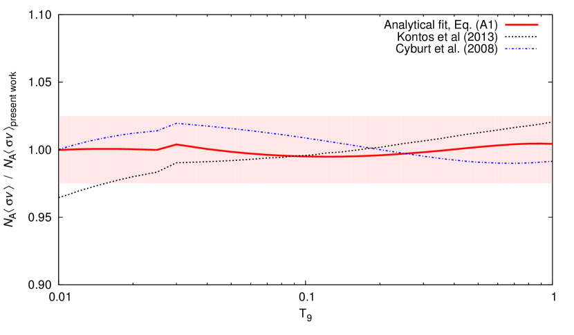
Figure 2: Thermonuclear reaction rate for the ³He($\alpha,\gamma$)⁷Be reaction, relative to the present rate, by Kontos et al. (black dashed curve, Kontos et al. (2013)) and by Cyburt et al. (blue dot-dashed curve, Cyburt and Davids (2008)). The analytical fit function from Eq. (A) is also shown (red full curve).

The S-factor curve resulting from the combined fit described in the previous section (Fig. 1) has subsequently been used to compute the thermonuclear reaction rate $R_{34}$ for its range of applicability, i.e. for $0.001\leq T_{9}\leq 1.0$, which includes the relevant temperature range for BBN (sec. I and Fig. 2).

For higher temperatures $T_{9}>1.0$, the conclusions depend on the slope of the excitation function above 1 MeV. Different theoretical papers give different slopes for $E$ $>$ 1 MeV Kajino (1986); Mertelmeier and Hoffmann (1986); Nollett (2001); Neff (2011). However, this temperature range is irrelevant for BBN (sec. I) and thus excluded from consideration here. The tabulated reaction rate and an analytical fitting function can be found in the Appendix.

The new rate was then used as input in the PArthENoPE BBN code Pisanti et al. (2008). Among publicly available codes Smith et al. (1993); Pisanti et al. (2008), PArthENoPE incorporates the more recent reaction rate data. For the present purposes, the physics input to PArthENoPE was updated for the following three parameters: ³He($\alpha,\gamma$)⁷Be reaction rate (present work), baryonic density Planck Collaboration et al. (2014) and neutron lifetime Olive and Particle Data Group (2014). See also sec. II for the latter two parameters.

The resulting BBN lithium abundance is

$${}^{7}{\rm Li/H}=5.0\times 10^{-10}$$ (12)

By repeating the BBN calculation with the upper and lower limits given by the error on $R_{34}$, it is found that the present 2.5% error for $R_{34}$ contributes just 2.4% uncertainty to the error budget of ${}^{7}{\rm Li/H}$. This value is to be compared with a previous contribution of 5.3% that can be estimated by using the previous $R_{34}$ error Cyburt and Davids (2008) and the previous correlation coefficient Coc et al. (2014). The total uncertainty of ${}^{7}{\rm Li/H}$ has previously been estimated to be 8% Coc et al. (2014). When subtracting the previous $R_{34}$ contribution in quadrature and adding the present, new $R_{34}$ contribution, a new total relative uncertainty of 6% can be estimated for ${}^{7}{\rm Li/H}$, leading to a final value of ${}^{7}{\rm Li/H}=(5.0\pm 0.3)\times 10^{-10}$. However, this estimated total uncertainty still needs to be borne out in a full BBN calculation re-analyzing in detail also the error budget contributions by parameters other than $R_{34}$.

The present ${}^{7}{\rm Li/H}$ value is well above the so-called Spite plateau of lithium abundances Fields (2011), and even further above the lithium values or limits found in extremely metal-poor stars (Caffau et al., 2011, e.g.). The recent predicted lithium isotopic ratio Anders et al. (2014) does not change outside the error bar with the present new ⁷Li/H result, it remains ⁶Li/⁷Li = (1.5$\pm$0.3)$\times 10^{-5}$.

VII Summary and outlook

The astrophysical S-factor of the ³He($\alpha,\gamma$)⁷Be reaction rate has been determined from the measured ⁷Be solar neutrino flux, using the standard solar model. The new data point of $S_{34}^{{}^{7}\text{Be}}(23^{+6}_{-5}\,\text{keV})$ = 0.548$\pm$0.054 keV b was then used to re-evaluate the excitation function in the energy range relevant for Big Bang nucleosynthesis. A combined average of $S_{34}(0)=0.561\pm$0.014 keV b is found.

Using the new excitation function, the ³He($\alpha,\gamma$)⁷Be thermonuclear reaction rate was re-computed for the Big Bang energy range, and the fit coefficients for the new recommended rate are given.

The present results are consistent with, but more precise than previous evaluations. The precision of this solar neutrino based approach will increase even further once the puzzle given by the solar elemental abundances is solved.

*

Appendix A Tabulated values and parameterization of the reaction rate

The reaction rate (Table 5) is reproduced within $\pm$0.5% for $0.01<T_{9}<1.0$ (Fig. 2) by the following analytical function:

$$R_{34} = p_{1}{T_{9}}^{-\frac{2}{3}}\exp(p_{2}{T_{9}}^{-\frac{1}{3}})\times$$

$$(1+p_{3}T_{9}+p_{4}T_{9}^{2}+p_{5}T_{9}^{3}+p_{6}T_{9}^{4})$$

The fit parameters are given in Table 4.

$p_{1}$	=	5.497	$\times 10^{6}$
$p_{2}$	=	-1.281	$\times 10^{1}$
$p_{3}$	=	-2.335	$\times 10^{-1}$
$p_{4}$	=	5.108	$\times 10^{-2}$
$p_{5}$	=	-1.672	$\times 10^{-3}$
$p_{6}$	=	-4.724	$\times 10^{-4}$

Table 4: Coefficients for the reaction rate fit in Eq. A.

$T_{9}$	Reaction rate	$T_{9}$	Reaction rate
0.001	$1.339\times 10^{-47}$	0.07	$1.013\times 10^{-6}$
0.002	$2.475\times 10^{-36}$	0.08	$3.581\times 10^{-6}$
0.003	$7.147\times 10^{-31}$	0.09	$1.038\times 10^{-5}$
0.004	$1.975\times 10^{-27}$	0.10	$2.589\times 10^{-5}$
0.005	$5.518\times 10^{-25}$	0.11	$5.747\times 10^{-5}$
0.006	$4.040\times 10^{-23}$	0.12	$1.162\times 10^{-4}$
0.007	$1.243\times 10^{-21}$	0.13	$2.178\times 10^{-4}$
0.008	$2.096\times 10^{-20}$	0.14	$3.832\times 10^{-4}$
0.009	$2.279\times 10^{-19}$	0.15	$6.398\times 10^{-4}$
0.010	$1.778\times 10^{-18}$	0.16	$1.021\times 10^{-3}$
0.011	$1.071\times 10^{-17}$	0.18	$2.331\times 10^{-3}$
0.012	$5.240\times 10^{-17}$	0.20	$4.731\times 10^{-3}$
0.013	$2.166\times 10^{-16}$	0.25	$1.936\times 10^{-2}$
0.014	$7.789\times 10^{-16}$	0.30	$5.619\times 10^{-2}$
0.015	$2.490\times 10^{-15}$	0.35	$1.306\times 10^{-1}$
0.016	$7.203\times 10^{-15}$	0.40	$2.606\times 10^{-1}$
0.018	$4.712\times 10^{-14}$	0.45	$4.652\times 10^{-1}$
0.020	$2.372\times 10^{-13}$	0.50	$7.636\times 10^{-1}$
0.025	$6.018\times 10^{-12}$	0.60	$1.714\times 10^{0}$
0.03	$7.019\times 10^{-11}$	0.70	$3.243\times 10^{0}$
0.04	$2.515\times 10^{-9}$	0.80	$5.454\times 10^{0}$
0.05	$3.177\times 10^{-8}$	0.90	$8.422\times 10^{0}$
0.06	$2.184\times 10^{-7}$	1.00	$1.220\times 10^{1}$

Table 5: ³He($\alpha,\gamma$)⁷Be reaction rate in cm³s^-1mole^-1.