Improved minimax estimation of a multivariate normal mean under heteroscedasticity

Abstract

Consider the problem of estimating a multivariate normal mean with a known variance matrix, which is not necessarily proportional to the identity matrix. The coordinates are shrunk directly in proportion to their variances in Efron and Morris’ (J. Amer. Statist. Assoc. 68 (1973) 117–130) empirical Bayes approach, whereas inversely in proportion to their variances in Berger’s (Ann. Statist. 4 (1976) 223–226) minimax estimators. We propose a new minimax estimator, by approximately minimizing the Bayes risk with a normal prior among a class of minimax estimators where the shrinkage direction is open to specification and the shrinkage magnitude is determined to achieve minimaxity. The proposed estimator has an interesting simple form such that one group of coordinates are shrunk in the direction of Berger’s estimator and the remaining coordinates are shrunk in the direction of the Bayes rule. Moreover, the proposed estimator is scale adaptive: it can achieve close to the minimum Bayes risk simultaneously over a scale class of normal priors (including the specified prior) and achieve close to the minimax linear risk over a corresponding scale class of hyper-rectangles. For various scenarios in our numerical study, the proposed estimators with extreme priors yield more substantial risk reduction than existing minimax estimators.

1 Introduction

A fundamental statistical problem is shrinkage estimation of a multivariate normal mean. See, for example, the February 2012 issue of Statistical Science for a broad range of theory, methods, and applications. Let $X=(X_{1},\ldots,X_{p})^{\mathrm{T}}$ be multivariate normal with unknown mean vector $\theta=(\theta_{1},\ldots,\theta_{p})^{\mathrm{T}}$ and known variance matrix $\Sigma$. Consider the problem of estimating $\theta$ by an estimator $\delta=\delta(X)$ under the loss $L(\delta,\theta)=(\delta-\theta)^{\mathrm{T}}Q(\delta-\theta)$, where $Q$ is a known positive definite, symmetric matrix. The risk of $\delta$ is $R(\delta,\theta)=E_{\theta}\{L(\delta,\theta)\}$. The general problem can be transformed into a canonical form such that $\Sigma$ is diagonal and $Q=I$, the identity matrix (e.g., Lehmann and Casella [21], Problem 5.5.11). For simplicity, assume except in Section 3.2 that $\Sigma$ is $D=\operatorname{diag}(d_{1},\ldots,d_{p})$ and $L(\delta,\theta)=\|\delta-\theta\|^{2}$, where $\|x\|^{2}=x^{\mathrm{T}}x$ for a column vector $x$. The letter $D$ is substituted for $\Sigma$ to emphasize that it is diagonal.

For this problem, we aim to develop shrinkage estimators that are both minimax and capable of effective risk reduction over the usual estimator $\delta_{0}=X$ even in the heteroscedastic case (i.e., $d_{1},\ldots,d_{p}$ are not equal). An estimator of $\theta$ is minimax if and only if, regardless of $\theta\in\mathbb{R}^{p}$, its risk is always no greater than $\sum_{j=1}^{p}d_{j}$, the risk of $\delta_{0}$. For $p\geq 3$, minimax estimators different from and hence dominating $\delta_{0}$ are first discovered in the homoscedastic case where $D=\sigma^{2}I$ (i.e., $d_{1}=\cdots=d_{p}=\sigma^{2}$). James and Stein [19] showed that $\delta_{c}^{\mathrm{JS}}=(1-c\sigma^{2}/\|X\|^{2})X$ is minimax provided $0\leq c\leq 2(p-2)$. Stein [26] suggested the positive-part estimator $\delta_{c}^{\mathrm{JS}+}=(1-c\sigma^{2}/\|X\|^{2})_{+}X$, which dominates $\delta_{c}^{\mathrm{JS}}$. Throughout, $a_{+}=\max(0,a)$. Shrinkage estimation has since been developed into a general methodology with various approaches, including empirical Bayes (Efron and Morris [17]; Morris [22]) and hierarchical Bayes (Strawderman [28]; Berger and Robert [7]). While these approaches are prescriptive for constructing shrinkage estimators, minimaxity is not automatically achieved but needs to be checked separately.

For the heteroscedastic case, there remain challenging issues on how much observations with different variances should be shrunk relatively to each other (e.g., Casella [15], Morris [22]). For the empirical Bayes approach (Efron and Morris [17]), the coordinates of $X$ are shrunk directly in proportion to their variances. But the existing estimators are, in general, non-minimax (i.e., may have a greater risk than the usual estimator $\delta_{0}$). On the other hand, Berger [3] proposed minimax estimators, including admissible minimax estimators, such that the coordinates of $X$ are shrunk inversely in proportion to their variances. But the risk reduction achieved over $\delta_{0}$ is insubstantial unless all the observations have similar variances.

To address the foregoing issues, we develop novel minimax estimators for multivariate normal means under heteroscedasticity. There are two central ideas in our approach. The first is to develop a class of minimax estimators by generalizing a geometric argument essentially in Stein [25] (see also Brandwein and Strawderman [11]). For the homoscedastic case, the argument shows that $\delta_{c}^{\mathrm{JS}}$ can be derived as an approximation to the best linear estimator of the form $(1-\lambda)X$, where $\lambda$ is a scalar. In fact, the optimal choice of $\lambda$ in minimizing the risk is $p\sigma^{2}/E_{\theta}(\|X\|^{2})$. Replacing $E_{\theta}(\|X\|^{2})$ by $\|X\|^{2}$ leads to $\delta_{c}^{\mathrm{JS}}$ with $c=p$. This derivation is highly informative, even though it does not yield the optimal value $c=p-2$.

Our class of minimax estimators are of the linear form $(I-\lambda A)X$, where $A$ is a nonnegative definite, diagonal matrix indicating the direction of shrinkage and $\lambda$ is a scalar indicating the magnitude of shrinkage. The matrix $A$ is open to specification, depending on the variance matrix $D$ but not on the data $X$. For a fixed $A$, the scalar $\lambda$ is determined to achieve minimaxity, depending on both $D$ and $X$. Berger’s [3] minimax estimator corresponds to the special choice $A=D^{-1}$, thereby leading to the unusual pattern of shrinkage discussed above.

The second idea of our approach is to choose $A$ by approximately minimizing the Bayes risk with a normal prior in our class of minimax estimators. The Bayes risk is used to measure average risk reduction for $\theta$ in an elliptical region as in Berger [4, 5]. It turns out that the solution of $A$ obtained by our approximation strategy has an interesting simple form. In fact, the coordinates of $X$ are automatically segmented into two groups, based on their Bayes “importance” (Berger [5]), which is of the same order as the coordinate variances when the specified prior is homoscedastic. The coordinates of high Bayes “importance” are shrunk inversely in proportion to their variances, whereas the remaining coordinates are shrunk in the direction of the Bayes rule. This shrinkage pattern may appear paradoxical: it may be expected that the coordinates of high Bayes “importance” are to be shrunk in the direction of the Bayes rule. But that scheme is inherently aimed at reducing the Bayes risk under the specified prior and, in general, fails to achieve minimaxity (i.e., it may lead to even a greater risk than the usual estimator $\delta_{0}$).

In addition to simplicity and minimaxity, we further show that the proposed estimator is scale adaptive in reducing the Bayes risk: it achieves close to the minimum Bayes risk, with the difference no greater than the sum of the 4 highest Bayes “importance” of the coordinates of $X$, simultaneously over a scale class of normal priors (including the specified prior). To our knowledge, the proposed estimator seems to be the first one with such a property in the general heteroscedastic case. Previously, in the homoscedastic case, $\delta_{p-2}^{\mathrm{JS}}$ is known to achieve the minimum Bayes risk up to the sum of 2 (equal-valued) Bayes “importance” of the coordinates over the scale class of homoscedastic normal priors (Efron and Morris [17]).

The rest of this article is organized as follows. Section 2 gives a review of existing estimators. Section 3 develops the new approach and studies risk properties of the proposed estimator. Section 4 presents a simulation study. Section 5 provides concluding remarks. All proofs are collected in the Appendix.

2 Existing estimators

We describe a number of existing shrinkage estimators. See Lehmann and Casella [21] for a textbook account and Strawderman [29] and Morris and Lysy [23] for recent reviews. Throughout, $\operatorname{tr}(\cdot)$ denotes the trace and $\lambda_{\max}(\cdot)$ denotes the largest eigenvalue. Then $\operatorname{tr}(D)=\sum_{j=1}^{p}d_{j}$ and $\lambda_{\max}(D)=\max(d_{1},\ldots,d_{p})$.

For a Bayes approach, assume the prior distribution: $\theta\sim\mathrm{N}(0,\gamma I)$, where $\gamma$ is the prior variance. The Bayes rule is given componentwise by $\delta^{\mathrm{Bayes}}_{j}=\{1-d_{j}/(d_{j}+\gamma)\}X_{j}$. Then the greater $d_{j}$ is, the more $X_{j}$ is shrunk whether $\gamma$ is fixed or estimated from the data. For the empirical Bayes approach of Efron and Morris [17], $\gamma$ is estimated by the maximum likelihood estimator $\hat{\gamma}$ such that

$$\hat{\gamma}=\sum_{j=1}^{p}\frac{X_{j}^{2}-d_{j}}{(d_{j}+\hat{\gamma})^{2}}\biggl{/}\sum_{j=1}^{p}\frac{1}{(d_{j}+\hat{\gamma})^{2}}.$$ (1)

Morris [22] suggested the modified estimator

$$\delta^{\mathrm{EB}}_{j}=\biggl{(}1-\frac{p-2}{p}\frac{d_{j}}{d_{j}+\hat{\gamma}_{+}}\biggr{)}X_{j}.$$ (2)

In our implementation, the right-hand side of (1) is computed to update $\hat{\gamma}$ from the initial guess, $p^{-1}\{\sum_{j=1}^{p}(X_{j}^{2}-d_{j})\}_{+}$, for up to 100 iterations until the successive absolute difference in $\hat{\gamma}$ is $\leq$$10^{-4}$, or $\hat{\gamma}$ is set to $\infty$ so that $\delta^{\mathrm{EB}}=X$ otherwise.

Alternatively, Xie et al. [31] proposed empirical Bayes-type estimators based on minimizing Stein’s [27] unbiased risk estimate (SURE) under heteroscedasticity. Their basic estimator is defined componentwise by

$$\delta^{\mathrm{XKB}}_{j}=\biggl{(}1-\frac{d_{j}}{d_{j}+\tilde{\gamma}}\biggr{)}X_{j},$$ (3)

where $\tilde{\gamma}$ is obtained by minimizing the SURE of $\delta^{\mathrm{Bayes}}$, that is, $\operatorname{SURE}(\gamma)=X^{\mathrm{T}}D\{D+\gamma I\}^{-1}X+2\gamma\operatorname{tr}\{D(D+\gamma I)^{-1}\}-\operatorname{tr}(D)$. In general, the two types of empirical Bayes estimators, $\delta^{\mathrm{EB}}$ and $\delta^{\mathrm{XKB}}$, are non-minimax, as shown in Section 4.

For a direct extension of $\delta_{c}^{\mathrm{JS}}$, consider the estimator $\delta_{c}^{\mathrm{S}}=(1-c/\|X\|^{2})X$ and, more generally, $\delta_{r}^{\mathrm{S}}=\{1-r(\|X\|^{2})/\|X\|^{2}\}X$, where $c$ is a scalar constant and $r(\cdot)$ a scalar function. See Lehmann and Casella [21], Theorem 5.7, although there are some typos. Both $\delta_{c}^{\mathrm{S}}$ and $\delta_{r}^{\mathrm{S}}$ are spherically symmetric. The estimator $\delta_{c}^{\mathrm{S}}$ is minimax provided

$$0\leq c\leq 2\bigl{\{}\operatorname{tr}(D)-2\lambda_{\max}(D)\bigr{\}},$$ (4)

and $\delta_{r}^{\mathrm{S}}$ is minimax provided $0\leq r(\cdot)\leq 2\{\operatorname{tr}(D)-2\lambda_{\max}(D)\}\mbox{ and }r(\cdot)\mbox{ is nondecreasing}$. No such $c\neq 0$ exists unless $\operatorname{tr}(D)>2\lambda_{\max}(D)$, which restricts how much $(d_{1},\ldots,d_{p})$ can differ from each other. For example, condition (4) fails when $p=10$ and

$$d_{1}=40,\qquad d_{2}=20,\qquad d_{3}=10,\qquad d_{4}=\cdots=d_{10}=1,$$ (5)

because $\operatorname{tr}(D)=77$ and $\lambda_{\max}(D)=40$.

Berger [3] proposed estimators of the form $\delta_{c}^{\mathrm{B}}=\{I-cD^{-1}/(X^{\mathrm{T}}D^{-2}X)\}X$ and $\delta_{r}^{\mathrm{B}}=\{I-r(X^{\mathrm{T}}D^{-2}X)/(X^{\mathrm{T}}D^{-2}X)D^{-1}\}X$, where $c$ is a scalar constant and $r(\cdot)$ a scalar function. Then $\delta_{c}^{\mathrm{B}}$ is minimax provided $0\leq c\leq 2(p-2)$, and $\delta_{r}^{\mathrm{B}}$ is minimax provided $0\leq r(\cdot)\leq 2(p-2)\mbox{ and }r(\cdot)\mbox{ is nondecreasing}$, regardless of differences between $(d_{1},\ldots,d_{p})$. However, a striking feature of $\delta_{c}^{\mathrm{B}}$ and $\delta_{r}^{\mathrm{B}}$, compared with $\delta^{\mathrm{EB}}$ and $\delta^{\mathrm{XKB}}$, is that the smaller $d_{j}$ is, the more $X_{j}$ is shrunk. For example (5), under $\delta_{c}^{\mathrm{B}}$, the coordinates $(X_{1},X_{2},X_{3})$ are shrunk only slightly, whereas $(X_{4},\ldots,X_{10})$ are shrunk as if they were shrunk as a 7-dimensional vector under $\delta_{c}^{\mathrm{JS}}$. The associated risk reduction is insubstantial, because the risk of estimating $(\theta_{4},\ldots,\theta_{10})$ is a small fraction of the overall risk of estimating $\theta$.

Define the positive-part version of $\delta_{c}^{\mathrm{B}}$ componentwise as

$$\bigl{(}\delta_{c}^{\mathrm{B}+}\bigr{)}_{j}=\biggl{(}1-\frac{cd_{j}^{-1}}{X^{\mathrm{T}}D^{-2}X}\biggr{)}_{+}X_{j}.$$ (6)

The estimator $\delta_{c}^{\mathrm{B}+}$ dominates $\delta_{c}^{\mathrm{B}}$ by Baranchik [1], Section 2.5. Berger [6], Equation (5.32), stated a different positive-part estimator, $\delta_{r}^{\mathrm{B}}$ with $r(t)=\min(p-2,t)$, but the $j$th component may not be of the same sign as $X_{j}$.

Given a prior $\theta\sim\mathrm{N}(0,\Gamma)$, Berger [5] suggested an approximation of Berger’s [4] robust generalized Bayes estimator as

$$\delta^{\mathrm{RB}}=\biggl{[}I-\min\biggl{\{}1,\frac{p-2}{X^{\mathrm{T}}(D+\Gamma)^{-1}X}\biggr{\}}D(D+\Gamma)^{-1}\biggr{]}X.$$ (7)

The estimator is expected to provide significant risk reduction over $\delta_{0}=X$ if the prior is correct and be robust to misspecification of the prior, but it is, in general, non-minimax. In the case of $\Gamma=0$, $\delta^{\mathrm{RB}}$ becomes $\{1-(p-2)/(X^{\mathrm{T}}D^{-1}X)\}_{+}X$, in the form of spherically symmetric estimators $\delta^{\mathrm{SS}}_{r}=\{1-r(X^{\mathrm{T}}D^{-1}X)/(X^{T}D^{-1}X)\}X$, where $r(\cdot)$ is a scalar function (Bock [10], Brown [12]). The estimator $\delta_{r}^{\mathrm{SS}}$ is minimax provided $0\leq r(\cdot)\leq 2\{\operatorname{tr}(D)/\lambda_{\max}(D)-2\}$ and $r(\cdot)$ is nondecreasing. Moreover, if $\operatorname{tr}(D)\leq 2\lambda_{\max}(D)$, then $\delta_{r}^{\mathrm{SS}}$ is non-minimax unless $r(\cdot)=0$.

To overcome the non-minimaxity of $\delta^{\mathrm{RB}}$, Berger [5] developed a minimax estimator $\delta^{\mathrm{MB}}$ by combining $\delta_{r}^{\mathrm{B}}$, $\delta^{\mathrm{RB}}$, and a minimax estimator of Bhattacharya [9]. Suppose that $\Gamma=\operatorname{diag}(\gamma_{1},\ldots,\gamma_{p})$ and the indices are sorted such that $d_{1}^{*}\geq\cdots\geq d_{p}^{*}$, where $d_{j}^{*}=d_{j}^{2}/(d_{j}+\gamma_{j})$. Define $\delta^{\mathrm{MB}}$ componentwise as

$$\delta^{\mathrm{MB}}_{j}=X_{j}-\Biggl{[}\frac{1}{d_{j}^{*}}\sum_{k=j}^{p}\bigl{(}d_{k}^{*}-d_{k+1}^{*}\bigr{)}\min\biggl{\{}1,\frac{(k-2)_{+}}{\sum_{\ell=1}^{k}X_{\ell}^{2}/(d_{\ell}+\gamma_{\ell})}\biggr{\}}\Biggr{]}\frac{d_{j}}{d_{j}+\gamma_{j}}X_{j},$$ (8)

where $d_{p+1}^{*}=0$. In the case of $\Gamma=0$, $\delta^{\mathrm{MB}}$ reduces to the original estimator of Bhattacharya [9]. The factor $(k-2)_{+}$ is replaced by $2(k-2)_{+}$ in Berger’s [5] original definition of $\delta^{\mathrm{MB}}$, corresponding to replacing $p-2$ by $2(p-2)$ in $\delta^{\mathrm{RB}}$. In our simulations, the two versions of $\delta^{\mathrm{MB}}$ somehow yield rather different risk curves, and so do the corresponding versions of other estimators. But there has been limited theory supporting one version over the other. Therefore, we focus on comparisons of only the corresponding versions of $\delta^{\mathrm{MB}}$ and other estimators.

3 Proposed approach

We develop a useful approach for shrinkage estimation under heteroscedasticity, by making explicit how different coordinates are shrunk differently. The approach not only sheds new light on existing results, but also lead to new minimax estimators.

3.1 A sketch

Assume that $\Sigma=D$ (diagonal) and $Q=I$. Consider estimators of the linear form

$$\delta=(I-\lambda A)X=X-\lambda AX,$$ (9)

where $A$ is a nonnegative definite, diagonal matrix indicating the direction of shrinkage and $\lambda$ is a scalar indicating the magnitude of shrinkage. Both $A$ and $\lambda$ are to be determined. A sketch of our approach is as follows.

1. [(iii)]

2. For a fixed $A$, the optimal choice of $\lambda$ in minimizing the risk is

   $$\lambda_{\mathrm{opt}}=\frac{\operatorname{tr}(DA)}{E_{\theta}(X^{\mathrm{T}}A^{\mathrm{T}}AX)}.$$

3. For a fixed $A$ and a scalar constant $c\geq 0$, consider the estimator

   $$\delta_{A,c}=X-\frac{c}{X^{\mathrm{T}}A^{\mathrm{T}}AX}AX.$$

   By Theorem 1, an upper bound on the risk function of $\delta_{A,c}$ is

   $$R(\delta_{A,c},\theta)\leq\operatorname{tr}(D)+E_{\theta}\biggl{[}\frac{c\{c-2c^{*}(D,A)\}}{X^{\mathrm{T}}A^{\mathrm{T}}AX}\biggr{]},$$ (10)

   where $c^{*}(D,A)=\operatorname{tr}(DA)-2\lambda_{\max}(DA)$. Requiring the second term to be no greater than 0 shows that if $c^{*}(D,A)\geq 0$, then $\delta_{A,c}$ is minimax provided

   $$0\leq c\leq 2c^{*}(D,A).$$ (11)

   If $c^{*}(D,A)\geq 0$, then the upper bound (10) has a minimum at $c=c^{*}(D,A)$.

4. By taking $c=c^{*}(D,A)$ in $\delta_{A,c}$, consider the estimator

   $$\delta_{A}=X-\frac{c^{*}(D,A)}{X^{\mathrm{T}}A^{\mathrm{T}}AX}AX$$

   subject to $c^{*}(D,A)\geq 0$, so that $\delta_{A}$ is minimax by step (ii). A positive-part estimator dominating $\delta_{A}$ is defined componentwise by

   $$\bigl{(}\delta_{A}^{+}\bigr{)}_{j}=\biggl{\{}1-\frac{c^{*}(D,A)a_{j}}{X^{\mathrm{T}}A^{\mathrm{T}}AX}\biggr{\}}_{+}X_{j},$$ (12)

   where $(a_{1},\ldots,a_{p})$ are the diagonal elements of $A$. The upper bound (10) on the risk functions of $\delta_{A}$ and $\delta^{+}_{A}$, subject to $c^{*}(D,A)\geq 0$, gives

   $$R(\delta_{A},\theta)\leq\operatorname{tr}(D)-E_{\theta}\biggl{\{}\frac{{c^{*}}^{2}(D,A)}{X^{\mathrm{T}}A^{\mathrm{T}}AX}\biggr{\}}.$$ (13)

   We propose to choose $A$ based on some optimality criterion, such as minimizing the Bayes risk with a normal prior centered at 0 (Berger [5]).

Further discussions of steps (i)–(iii) are provided in Sections 3.2–3.3.

3.2 Constructing estimators: Steps (i)–(ii)

We first develop steps (i)–(ii) for the general problem where neither $\Sigma$ nor $Q$ may be diagonal. The results can be as concisely stated as those just presented for the canonical problem where $\Sigma$ is diagonal and $Q=I$. Such a unification adds to the attractiveness of the proposed approach.

Consider estimators of the form (9), where $A$ is not necessarily diagonal, but

$$A\Sigma\mbox{ is nonnegative definite.}$$ (14)

Condition (14) is invariant under a linear transformation. To see this, let $B$ be a nonsingular matrix and $\Sigma^{*}=B\Sigma B^{\mathrm{T}}$ and $A^{*}=BAB^{-1}$. For the transformed problem of estimating $\theta^{*}=B\theta$ based on $X^{*}=BX$ with variance matrix $\Sigma^{*}$, the transformed estimator from (9) is $\delta^{*}=X^{*}-\lambda A^{*}X^{*}$. The application of condition (14) to $\delta^{*}$ says that $A^{*}\Sigma^{*}=BA\Sigma B^{\mathrm{T}}$ is nonnegative definite and therefore is equivalent to (14) itself. For the canonical problem where $\Sigma=D$ (diagonal), condition (14) only requires that $AD$ is nonnegative definite, allowing $A$ to be non-diagonal. On the other hand, it seems intuitively appropriate to restrict $A$ to be diagonal. Then condition (14) is equivalent to saying that $A$ is nonnegative definite (and diagonal), which is the condition introduced on $A$ in the sketch in Section 3.1.

The risk of an estimator of the form (9) is

$$E_{\theta}\bigl{\{}(X-\theta-\lambda AX)^{\mathrm{T}}Q(X-\theta-\lambda AX)\bigr{\}}$$

$$\quad=E_{\theta}\bigl{\{}(X-\theta)^{\mathrm{T}}Q(X-\theta)\bigr{\}}+\lambda^{2}E_{\theta}\bigl{(}X^{\mathrm{T}}A^{\mathrm{T}}QAX\bigr{)}-2\lambda E_{\theta}\bigl{\{}(X-\theta)^{\mathrm{T}}QAX\bigr{\}}.$$

For a fixed $A$, the optimal $\lambda$ in minimizing the risk is

$$\lambda_{\mathrm{opt}}=\frac{E_{\theta}\{(X-\theta)^{\mathrm{T}}QAX\}}{E_{\theta}(X^{\mathrm{T}}A^{\mathrm{T}}QAX)}=\frac{\operatorname{tr}(\Sigma QA)}{E_{\theta}(X^{\mathrm{T}}A^{\mathrm{T}}QAX)}.$$

Replacing $E_{\theta}(X^{\mathrm{T}}A^{\mathrm{T}}QAX)$ by $X^{\mathrm{T}}A^{\mathrm{T}}QAX$ and $\operatorname{tr}(\Sigma QA)$ by a scalar constant $c\geq 0$ leads to the estimator

$$\delta_{A,c}=X-\frac{c}{X^{\mathrm{T}}A^{\mathrm{T}}QAX}AX.$$

For a generalization, replacing $c$ by $r(X^{\mathrm{T}}A^{\mathrm{T}}QAX)$ with a scalar function $r(\cdot)\geq 0$ leads to the estimator

$$\delta_{A,r}=X-\frac{r(X^{\mathrm{T}}A^{\mathrm{T}}QAX)}{X^{\mathrm{T}}A^{\mathrm{T}}QAX}AX.$$

We provide in Theorem 1 an upper bound on the risk function of $\delta_{A,r}$.

Theorem 1

Assume that $r(\cdot)$ almost differentiable (Stein [27]). If (14) holds and $r(\cdot)\geq 0$ is nondecreasing, then for each $\theta$,

$$R(\delta_{A,r},\theta)\leq\operatorname{tr}(\Sigma Q)+E_{\theta}\biggl{[}\frac{r\{r-2c^{*}(\Sigma,Q,A)\}}{X^{\mathrm{T}}A^{\mathrm{T}}QAX}\biggr{]},$$ (15)

where $r=r(X^{\mathrm{T}}A^{\mathrm{T}}QAX)$ and $c^{*}(\Sigma,Q,A)=\operatorname{tr}(A\Sigma Q)-\lambda_{\max}(A\Sigma Q+\Sigma A^{\mathrm{T}}Q)$. Taking $r(\cdot)\equiv c\geq 0$ in (15) gives an upper bound on $R(\delta_{A,c},\theta)$.

Requiring the second term in the risk upper bound (15) to be no greater than 0 leads to a sufficient condition for $\delta_{A,r}$ to be minimax.

Corollary 1

If (14) holds and $c^{*}(\Sigma,Q,A)\geq 0$, then $\delta_{A,r}$ is minimax provided

$$0\leq r(\cdot)\leq 2c^{*}(\Sigma,Q,A)\quad\mbox{and}\quad r(\cdot)\mbox{ is nondecreasing}.$$ (16)

Particularly, $\delta_{A,c}$ is minimax provided $0\leq c\leq 2c^{*}(\Sigma,Q,A)$.

For the canonical problem, inequality (15) and condition (16) for $\delta_{A,c}$ give respectively (10) and (11). These results generalize the corresponding ones for $\delta_{c}^{\mathrm{S}}$ and $\delta_{c}^{\mathrm{B}}$ in Section 2, by the specific choices $A=I$ or $D^{-1}$. The generalization also holds if $c$ is replaced by a scalar function $r(\cdot)>0$. In fact, condition (16) reduces to Baranchik’s [2] condition in the homoscedastic case.

If $c^{*}(\Sigma,Q,A)\geq 0$, then the risk upper bound (15) has a minimum at $r(\cdot)\equiv c=c^{*}(\Sigma,Q,A)$. As a result, consider the estimator

$$\delta_{A}=X-\frac{c^{*}(\Sigma,Q,A)}{X^{\mathrm{T}}A^{\mathrm{T}}QAX}AX,$$

which is minimax provided $c^{*}(\Sigma,Q,A)\geq 0$. If $A=Q^{-1}\Sigma^{-1}$ (Berger [3]), then $c^{*}(\Sigma,Q,A)=p-2$ and, by the proof of Theorem 1 in the Appendix, the risk upper bound (15) becomes exact for $\delta_{A,c}$. Therefore, for $A=Q^{-1}\Sigma^{-1}$, the estimator $\delta_{A}=\delta_{A,p-2}$ is uniformly best in the class $\delta_{A,c}$, in agreement with the result that $\delta_{p-2}^{\mathrm{JS}}$ is uniformly best among $\delta_{c}^{\mathrm{JS}}$ in the homoscedastic case.

The estimator $\delta_{A}$ has desirable properties of invariance. First, $\delta_{A}$ is easily shown to be invariant under a multiplicative transformation $A\mapsto aA$ for a scalar $a>0$. Second, $\delta_{A}$ is invariant under a linear transformation of the inference problem. Similarly as discussed below (14), let $B$ be a nonsingular matrix and $\Sigma^{*}=B\Sigma B^{\mathrm{T}}$, $Q^{*}={B^{\mathrm{T}}}^{-1}QB^{-1}$, and $A^{*}=BAB^{-1}$. For the transformed problem of estimating $\theta^{*}=B\theta$ based on $X^{*}=BX$, the transformed estimator from $\delta_{A}$ is $X^{*}-\{c^{*}(\Sigma,Q,A)/({X^{*}}^{\mathrm{T}}{A^{*}}^{\mathrm{T}}Q^{*}A^{*}X^{*})\}A^{*}X^{*}$, whereas the application of $\delta_{A}$ is $X^{*}-\{c^{*}(\Sigma^{*},Q^{*},A^{*})/({X^{*}}^{\mathrm{T}}{A^{*}}^{\mathrm{T}}Q^{*}A^{*}X^{*})\}A^{*}X^{*}$. The two estimators are identical because $A^{*}\Sigma^{*}Q^{*}=BA\Sigma QB^{-1}$, $\Sigma^{*}{A^{*}}^{\mathrm{T}}Q^{*}=B\Sigma A^{\mathrm{T}}QB^{-1}$, and hence $c^{*}(\Sigma^{*},Q^{*},A^{*})=c^{*}(\Sigma,Q,A)$.

Finally, we present a positive-part estimator dominating $\delta_{A}$ in the case where both $A\Sigma$ and $QA$ are symmetric, that is,

$$A\Sigma=\Sigma A^{\mathrm{T}}\quad\mbox{and}\quad QA=A^{\mathrm{T}}Q.$$ (17)

Similarly to (14), it is easy to see that this condition is invariant under a linear transformation. Condition (17) is trivially true if $\Sigma$, $Q$, and $A$ are diagonal. In the Appendix, we show that (17) holds if and only if there exists a nonsingular matrix $B$ such that $Q=B^{\mathrm{T}}B$, $\Sigma=B^{-1}D{B^{\mathrm{T}}}^{-1}$, and $A=B^{-1}A^{*}B$, where $D$ and $A^{*}$ are diagonal and the diagonal elements of $D$ or $A^{*}$ are, respectively, the eigenvalues of $\Sigma Q$ or $A$. In the foregoing notation, $\Sigma^{*}=D$ and $Q^{*}=I$. For the problem of estimating $\theta^{*}=B\theta$ based on $X^{*}=BX$, consider the estimator $\eta=X-\{c^{*}(D,A^{*})/({X^{*}}^{\mathrm{T}}{A^{*}}^{\mathrm{T}}A^{*}X^{*})\}A^{*}X$ and the positive-part estimator $\eta^{+}$ with the $j$th component,

$$\biggl{\{}1-\frac{c^{*}(D,A^{*})}{{X^{*}}^{\mathrm{T}}{A^{*}}^{\mathrm{T}}A^{*}X^{*}}a_{j}^{*}\biggr{\}}_{+}X^{*}_{j},$$

where $(a_{1}^{*},\ldots,a_{p}^{*})$ are the diagonal elements of $A^{*}$. The estimator $\eta^{+}$ dominates $\eta$ by a simple extension of Baranchik [1], Section 2.5. By a transformation back to the original problem, $\eta$ yields $\delta_{A}$, whereas $\eta^{+}$ yields

$$\delta_{A}^{+}=B^{-1}\operatorname{diag}\biggl{[}\biggl{\{}1-\frac{c^{*}(\Sigma,Q,A)}{X^{\mathrm{T}}A^{\mathrm{T}}QAX}a^{*}_{1}\biggr{\}}_{+},\ldots,\biggl{\{}1-\frac{c^{*}(\Sigma,Q,A)}{X^{\mathrm{T}}A^{\mathrm{T}}QAX}a^{*}_{p}\biggr{\}}_{+}\biggr{]}BX.$$

Then $\delta_{A}^{+}$ dominates $\delta_{A}$. Therefore, (15) also gives an upper bound on the risk of $\delta_{A}^{+}$, with $r(\cdot)\equiv c^{*}(\Sigma,Q,A)$, even though $\delta_{A}^{+}$ is not of the form $\delta_{A,r}$.

In practice, a matrix $A$ satisfying (17) can be specified in two steps. First, find a nonsingular matrix $B$ such that $Q=B^{\mathrm{T}}B$ and $\Sigma=B^{-1}D{B^{\mathrm{T}}}^{-1}$, where $D$ is diagonal. Second, pick a diagonal matrix $A^{*}$ and define $A=B^{-1}A^{*}B$. The first step is always feasible by taking $B=OC$, where $C$ is a nonsingular matrix such that $Q=C^{\mathrm{T}}C$ and $O$ is an orthogonal matrix $O$ such that $O(C\Sigma C^{\mathrm{T}})O^{\mathrm{T}}$ is diagonal. Given $(\Sigma,Q)$ and $D$, it can be shown that $A$ and $\delta_{A}^{+}$ depend on the choice of $A^{*}$, but not on that of $B$, provided that $a^{*}_{j}=a^{*}_{k}$ if $d_{j}=d_{k}$ for any $j,k=1,\ldots,p$. In the canonical case where $\Sigma=D$ and $Q=I$, this condition amounts to saying that any coordinates of $X$ with the same variances should be shrunk in the same way.

3.3 Constructing estimators: Step (iii)

Different choices of $A$ lead to different estimators $\delta_{A}$ and $\delta_{A}^{+}$. We study how to choose $A$, depending on $(\Sigma,Q)$ but not on $X$, to approximately optimize risk reduction while preserving minimaxity for $\delta_{A}$. The estimator $\delta_{A}^{+}$ provides even greater risk reduction than $\delta_{A}$. We focus on the canonical problem where $\Sigma=D$ (diagonal) and $Q=I$. Further, we restrict $A$ to be diagonal and nonnegative definite.

As discussed in Berger [4], any estimator can have significantly smaller risk than $\delta_{0}=X$ only for $\theta$ in a specific region. Berger [4, 5] considered the situation where significant risk reduction is desired for an elliptical region

$$\bigl{\{}\theta\colon\ (\theta-\mu)^{\mathrm{T}}\Gamma^{-1}(\theta-\mu)\leq p\bigr{\}},$$ (18)

with $\mu$ and $\Gamma$ the prior mean and prior variance matrix. See $\delta^{\mathrm{RB}}$ and $\delta^{\mathrm{MB}}$ reviewed in Section 2. To measure average risk reduction for $\theta$ in region (18), Berger [5] used the Bayes risk with the normal prior $\theta\sim\mathrm{N}(\mu,\Gamma)$. For simplicity, assume throughout that $\mu=0$ and $\Gamma=\operatorname{diag}(\gamma_{1},\ldots,\gamma_{p})$ is diagonal.

We adopt Berger’s [5] ideas of specifying an elliptical region and using the Bayes risk to quantify average risk reduction in this region. We aim to find $A$, subject to $c^{*}(D,A)\geq 0$, minimizing the Bayes risk of $\delta_{A}$ with the prior $\pi_{\Gamma}$, $\theta\sim\mathrm{N}(0,\Gamma)$,

$$R(\delta_{A},\pi_{\Gamma})=E^{\pi_{\Gamma}}E_{\theta}\bigl{(}\|\delta_{A}-\theta\|^{2}\bigr{)},$$

where $E^{\pi_{\Gamma}}$ denotes the expectation with respect to the prior $\pi_{\Gamma}$. Given $A$, the risk $R(\delta_{A},\pi_{\Gamma})$ can be numerically evaluated. A simple Monte Carlo method is to repeatedly draw $\theta\sim\mathrm{N}(0,\Gamma)$ and $X|\theta\sim\mathrm{N}(\theta,D)$ and then take the average of $\|\delta_{A}(X)-\theta\|^{2}$. But it seems difficult to literally implement the foregoing optimization. Alternatively, we develop a simple method for choosing $A$ by two approximations.

First, if $c^{*}(D,A)\geq 0$, then taking the expectation of both sides of (13) with respect to the prior $\pi_{\Gamma}$ gives an upper bound on the Bayes risk of $\delta_{A}$:

$$R(\delta_{A},\pi_{\Gamma})\leq\operatorname{tr}(D)-E^{m}\biggl{\{}\frac{{c^{*}}^{2}(D,A)}{X^{\mathrm{T}}A^{\mathrm{T}}AX}\biggr{\}},$$ (19)

where $E^{m}$ denotes the expectation with respect to the marginal distribution of $X$ in the Bayes model, that is, $X\sim\mathrm{N}(0,D+\Gamma)$. An approximation strategy for choosing $A$ is to minimize the upper bound (19) on the Bayes risk or to maximize the second term. The expectation $E^{m}\{(X^{\mathrm{T}}A^{\mathrm{T}}AX)^{-1}\}$ can be evaluated as a 1-dimensional integral by results on inverse moments of quadratic forms in normal variables (e.g., Jones [20]). But the required optimization problem remains difficult.

Second, approximations can be made to the distribution of the quadratic form $X^{\mathrm{T}}A^{\mathrm{T}}AX$. Suppose that $X^{\mathrm{T}}A^{\mathrm{T}}AX$ is approximated with the same mean by $\{\sum_{j=1}^{p}(d_{j}+\gamma_{j})a_{j}^{2}\}\chi^{2}_{p}/p$, where $\chi^{2}_{p}$ is a chi-squared variable with $p$ degrees of freedom. Then $E^{m}\{(X^{\mathrm{T}}A^{\mathrm{T}}AX)^{-1}\}$ is approximated by $\{p/(p-2)\}\{\sum_{j=1}^{p}(d_{j}+\gamma_{j})a_{j}^{2}\}^{-1}$. We show in the Appendix that this approximation gives a valid lower bound:

$$E^{m}\biggl{(}\frac{1}{X^{\mathrm{T}}A^{\mathrm{T}}AX}\biggr{)}\geq\frac{p}{p-2}\cdot\frac{1}{\sum_{j=1}^{p}(d_{j}+\gamma_{j})a_{j}^{2}}.$$ (20)

A direct application of Jensen’s inequality shows that $E^{m}\{(X^{\mathrm{T}}A^{\mathrm{T}}AX)^{-1}\}\geq\{\sum_{j=1}^{p}(d_{j}+\gamma_{j})a_{j}^{2}\}^{-1}$. But the lower bound (20) is strictly tighter and becomes exact when $(d_{1}+\gamma_{1})a_{1}^{2}=\cdots=(d_{p}+\gamma_{p})a_{p}^{2}$. No simple bounds such as (20) seem to hold if more complicated approximations (e.g., Satterthwaite [24]) are used.

Combining (19) and (20) shows that if $c^{*}(D,A)\geq 0$, then

$$R(\delta_{A},\pi_{\Gamma})\leq\operatorname{tr}(D)-\frac{p}{p-2}\cdot\frac{{c^{*}}^{2}(D,A)}{\sum_{j=1}^{p}(d_{j}+\gamma_{j})a_{j}^{2}}.$$ (21)

Notice that $\delta_{A}$ is invariant under a multiplicative transformation $A\mapsto aA$ for a scalar $a>0$, and so is the upper bound (21). Our strategy for choosing $A$ is to minimize the upper bound (21) subject to $c^{*}(D,A)\geq 0$ or, equivalently, to solve the constrained optimization problem:

$$\max_{A}\quad c^{*}(D,A)=\sum_{j=1}^{p}d_{j}a_{j}-2\max_{j=1,\ldots,p}d_{j}a_{j}$$

(22)

$$\quad\mbox{subject to}\quad\sum_{j=1}^{p}(d_{j}+\gamma_{j})a_{j}^{2}=\mbox{fixed}.$$

The condition $c^{*}(D,A)\geq 0$ is dropped, because for $p\geq 3$, the achieved maximum is at least $c^{*}(D,aD^{-1})=a(p-2)>0$ for some scalar $a>0$. In spite of the approximations used in our approach, Theorem 2 shows that not only the problem (3.3) admits a non-iterative solution, but also the solution has a very interesting interpretation. For convenience, assume thereafter that the indices are sorted such that $d_{1}^{2}/(d_{1}+\gamma_{1})\geq d_{2}^{2}/(d_{2}+\gamma_{2})\geq\cdots\geq d_{p}^{2}/(d_{p}+\gamma_{p})$.

Theorem 2

Assume that $p\geq 3$, $D=\operatorname{diag}(d_{1},\ldots,d_{p})$ with $d_{j}>0$ and $\Gamma=\operatorname{diag}(\gamma_{1},\ldots,\gamma_{p})$ with $\gamma_{j}\geq 0$ ($j=1,\ldots,p$). For problem (3.3), assume that $A=\operatorname{diag}(a_{1},\ldots,a_{p})$ with $a_{j}\geq 0$ ($j=1,\ldots,p$) and $\sum_{j=1}^{p}(d_{j}+\gamma_{j})a_{j}^{2}=\sum_{j=1}^{p}d_{j}^{2}/(d_{j}+\gamma_{j})$, satisfied by $a_{j}=d_{j}/(d_{j}+\gamma_{j})$. Then the following results hold.

1. [(iii)]

2. There exists a unique solution, $A^{\dagger}=\operatorname{diag}(a_{1}^{\dagger},\ldots,a_{p}^{\dagger})$, to problem (3.3).

3. Let $\nu$ be the largest index such that $d_{\nu}a^{\dagger}_{\nu}=\max(d_{1}a_{1}^{\dagger},\ldots,d_{p}a_{p}^{\dagger})$. Then $\nu\geq 3$, $d_{1}a_{1}^{\dagger}=\cdots=d_{\nu}a_{\nu}^{\dagger}>d_{j}a_{j}^{\dagger}$ for $j\geq\nu+1$, and

   $$a_{j}^{\dagger} = K_{\nu}\Biggl{(}\sum_{k=1}^{\nu}\frac{d_{k}+\gamma_{k}}{d_{k}^{2}}\Biggr{)}^{-1}\frac{\nu-2}{d_{j}}\qquad(j=1,\ldots,\nu),$$

   $$a_{j}^{\dagger} = K_{\nu}\frac{d_{j}}{d_{j}+\gamma_{j}}\qquad(j=\nu+1,\ldots,p),$$

   where $K_{\nu}=\{\sum_{j=1}^{p}d_{j}^{2}/(d_{j}+\gamma_{j})\}^{1/2}M_{\nu}^{-1/2}$ and

   $$M_{\nu}=\frac{(\nu-2)^{2}}{\sum_{j=1}^{\nu}(d_{j}+\gamma_{j})/d_{j}^{2}}+\sum_{j=\nu+1}^{p}\frac{d_{j}^{2}}{d_{j}+\gamma_{j}}.$$

   The achieved maximum value, $c^{*}(D,A^{\dagger})$, is $K_{\nu}M_{\nu}\ (>0)$.

4. The resulting estimator $\delta_{A^{\dagger}}$ is minimax.

We emphasize that, although $A$ can be considered a tuning parameter, the solution $A^{\dagger}$ is data independent, so that $\delta_{A^{\dagger}}$ is automatically minimax. If a data-dependent choice of $A$ were used, minimaxity would not necessarily hold. This result is achieved both because each estimator $\delta_{A}$ with $c^{*}(D,A)\geq 0$ is minimax and because a global criterion (such as the Bayes risk) is used, instead of a pointwise criterion (such as the frequentist risk at the unknown $\theta$), to select $A$. By these considerations, our approach differs from the usual exercise of selecting a tuning parameter in a data-dependent manner for a class of candidate estimators.

There is a remarkable property of monotonicity for the sequence $(M_{3},M_{4},\ldots,M_{p})$, which underlies the uniqueness of $\nu$ and $A^{\dagger}$.

Corollary 2

The sequence $(M_{3},M_{4},\ldots,M_{p})$ is nonincreasing: for $3\leq k\leq p-1$, $M_{k}\geq M_{k+1}$, where the equality holds if and only if

$$\frac{k-2}{\sum_{j=1}^{k}(d_{j}+\gamma_{j})/d_{j}^{2}}=\frac{d_{k+1}^{2}}{d_{k+1}+\gamma_{k+1}}.$$

The condition $d_{\nu}a_{\nu}^{\dagger}>d_{\nu+1}a_{\nu+1}^{\dagger}$ is equivalent to saying that the left side is greater than the right-hand side in the above expression for $k=\nu$. Therefore, $\nu$ is the smallest index $3\leq k\leq p-1$ with this property, and $M_{\nu}>M_{\nu+1}$.

The estimator $\delta_{A^{\dagger}}$ is invariant under scale transformations of $A^{\dagger}$. Therefore, the constant $K_{\nu}$ can be dropped from the expression of $A^{\dagger}$ in Theorem 1.

Corollary 3

The solution $A^{\dagger}=\operatorname{diag}(a_{1}^{\dagger},\ldots,a_{p}^{\dagger})$ can be rescaled such that

$$a_{j}^{\dagger} = \Biggl{(}\sum_{k=1}^{\nu}\frac{d_{k}+\gamma_{k}}{d_{k}^{2}}\Biggr{)}^{-1}\frac{\nu-2}{d_{j}}\qquad(j=1,\ldots,\nu),$$ (23)

$$a_{j}^{\dagger} = \frac{d_{j}}{d_{j}+\gamma_{j}}\qquad(j=\nu+1,\ldots,p).$$ (24)

Then $c^{*}(D,A^{\dagger})=\sum_{j=1}^{p}{a_{j}^{{\dagger}}}^{2}(d_{j}+\gamma_{j})=M_{\nu}$. Moreover, it holds that

$$a_{j}^{\dagger}\leq\frac{d_{j}}{d_{j}+\gamma_{j}}\qquad(j=1,\ldots,\nu).$$ (25)

The estimator $\delta_{A^{\dagger}}$ can be expressed as

$$\delta_{A^{\dagger}}=X-\frac{\sum_{j=1}^{p}{a_{j}^{{\dagger}}}^{2}(d_{j}+\gamma_{j})}{\sum_{j=1}^{p}{a_{j}^{{\dagger}}}^{2}X_{j}^{2}}A^{\dagger}X.$$ (26)

The foregoing results lead to a simple algorithm for solving problem (3.3):

1. [(iii)]

2. Sort the indices such that $d_{1}^{2}/(d_{1}+\gamma_{1})\geq\cdots\geq d_{p}^{2}/(d_{p}+\gamma_{p})$.

3. Take $\nu$ to be the smallest index $k$ (corresponding to the largest $M_{k}$) such that $3\leq k\leq p-1$ and

   $$\frac{k-2}{\sum_{j=1}^{k}(d_{j}+\gamma_{j})/d_{j}^{2}}>\frac{d_{k+1}^{2}}{d_{k+1}+\gamma_{k+1}},$$

   or take $\nu=p$ if there exists no such $k$.

4. Compute $(a_{1}^{\dagger},\ldots,a_{p}^{\dagger})$ by (23)–(24).

This algorithm is guaranteed to find the (unique) solution to problem (3.3) by a fixed number of numerical operations. No iteration or convergence diagnosis is required. Therefore, the algorithm is exact and non-iterative, in contrast with usual iterative algorithms for nonlinear, constrained optimization.

The estimator $\delta_{A^{\dagger}}$ has an interesting interpretation. By (23)–(24), there is a dichotomous segmentation in the shrinkage direction of the coordinates of $X$ based on $d_{j}^{*}=d_{j}^{2}/(d_{j}+\gamma_{j})$. This quantity $d_{j}^{*}$ is said to reflect the Bayes “importance” of $\theta_{j}$, that is, the amount of reduction in Bayes risk obtainable in estimating $\theta_{j}$ in Berger [5]. The coordinates with high $d_{j}^{*}$ are shrunk inversely in proportion to their variances $d_{j}$ as in Berger’s [3] estimator $\delta_{c}^{\mathrm{B}}$, whereas the coordinates with low $d_{j}^{*}$ are shrunk in the direction of the Bayes rule. Therefore, $\delta_{A^{\dagger}}$ mimics the Bayes rule to reduce the Bayes risk, except that $\delta_{A^{\dagger}}$ mimics $\delta_{c}^{\mathrm{B}}$ for some coordinates of highest Bayes “importance” in order to achieve minimaxity. In fact, by inequality (25), the relative shrinkage, $a_{j}^{\dagger}/\{d_{j}/(d_{j}+\gamma_{j})\}$, of each $X_{j}$ ($j=1,\ldots,\nu$) in $\delta_{A^{\dagger}}$ versus the Bayes rule is always no greater than that of $X_{k}$ ($k=\nu+1,\ldots,p$).

The expression (26) suggests that there is a close relationship in beyond the shrinkage direction between $\delta_{A^{\dagger}}$ and the Bayes rule under the Bayes model, $X\sim\mathrm{N}(0,D+\Gamma)$. In this case, $E^{m}(\sum_{j=1}^{p}{a_{j}^{{\dagger}}}^{2}X_{j}^{2})=\sum_{j=1}^{p}{a_{j}^{{\dagger}}}^{2}(d_{j}+\gamma_{j})$, and hence $\delta_{A^{\dagger}}$ behaves similarly to $X-A^{\dagger}X$. Therefore, on average under the Bayes model, the coordinates of $X$ are shrunk in $\delta_{A^{\dagger}}$ the same as in the Bayes rule, except that some coordinates of highest Bayes “importance” are shrunk no greater than in the Bayes rule. While this discussion seems heuristic, we provide in Section 3.4 a rigorous analysis of the Bayes risk of $\delta_{A^{\dagger}}$, compared with that of the Bayes rule.

We now examine $\delta_{A^{\dagger}}$ for two types of priors: $\gamma_{1}=\cdots=\gamma_{p}=\gamma$ and $\gamma_{j}=\gamma d_{j}$ ($j=1,\ldots,p$), referred to as the homoscedastic and heteroscedastic priors. For both types, $(d_{1}^{*},\ldots,d_{p}^{*})$ are of the same order as the variances $(d_{1},\ldots,d_{p})$. Recall that $\delta_{A}$ is invariant under a multiplicative transformation of $A$. For both the homoscedastic prior with $\gamma=0$ and the heteroscedastic prior regardless of $\gamma\geq 0$, the solution $A^{\dagger}=\operatorname{diag}(a_{1}^{\dagger},\ldots,a_{p}^{\dagger})$ can be rescaled such that

$$a_{j}^{\dagger} = \Biggl{(}\sum_{k=1}^{\nu}d_{k}^{-1}\Biggr{)}^{-1}\frac{\nu-2}{d_{j}}\qquad(j=1,\ldots,\nu),$$

$$a_{j}^{\dagger} = 1\qquad(j=\nu+1,\ldots,p).$$

Denote by $A^{\dagger}_{0}$ this rescaled matrix $A^{\dagger}$, corresponding to $\Gamma=0$. Then coordinates with high variances are shrunk inversely in proportion to their variances, whereas coordinates with low variances are shrunk symmetrically. For $\Gamma=0$, the proposed method has a purely frequentist interpretation: it seeks to minimize the upper bound (21) on the pointwise risk of $\delta_{A}$ at $\theta=0$.

For the homoscedastic prior with $\gamma\to\infty$, the proposed method is then to minimize the upper bound (21) on the Bayes risk of $\delta_{A}$ with an extremely flat, homoscedastic prior. As $\gamma\to\infty$, the solution $A^{\dagger}$ can be rescaled such that

$$a_{j}^{\dagger} = \Biggl{(}\sum_{k=1}^{\nu}d_{k}^{-2}\Biggr{)}^{-1}\frac{\nu-2}{d_{j}}\qquad(j=1,\ldots,\nu),$$

$$a_{j}^{\dagger} = d_{j}\qquad(j=\nu+1,\ldots,p).$$

Denote by $A^{\dagger}_{\infty}$ this rescaled matrix $A^{\dagger}$. Then coordinates with low (or high) variances are shrunk directly (or inversely) in proportion to their variances. The direction $A^{\dagger}_{\infty}$ can also be obtained by using a fixed prior in the form $\gamma_{j}=\gamma d_{1}-d_{j}$ ($j=1,\ldots,p$) for arbitrary $\gamma\geq 1$, where $d_{1}=\max_{j=1,\ldots,p}d_{j}$.

Finally, in the homoscedastic case ($d_{1}=\cdots=d_{p}=\sigma^{2}$), if the prior is also homoscedastic ($\gamma_{1}=\cdots=\gamma_{p}=\gamma$), then $\nu=p$, $a_{1}^{\dagger}=\cdots=a_{p}^{\dagger}$, and $\delta_{A^{\dagger}}$ reduces to the James–Stein estimator $\delta_{p-2}^{\mathrm{JS}}$, regardless of $\sigma^{2}$ and $\gamma$.

3.4 Evaluating estimators

The estimator $\delta_{A^{\dagger}}$ is constructed by minimizing the upper bound (21) on the Bayes risk subject to minimaxity. In addition to simplicity, interpretability, and minimaxity demonstrated for $\delta_{A^{\dagger}}$, it remains important to further study risk properties of $\delta_{A^{\dagger}}$ and show that $\delta_{A^{\dagger}}$ can provide effective risk reduction over $\delta_{0}=X$. Write $\delta_{A^{\dagger}}=\delta_{A^{\dagger}(\Gamma)}$ whenever needed to make explicit the dependency of $A^{\dagger}$ on $\Gamma$.

First, we study how close the Bayes risk of $\delta_{A^{\dagger}(\Gamma)}$ can be to that of the Bayes rule, which is the smallest possible among all estimators including non-minimax ones, under the prior $\pi_{\Gamma}$, $\theta\sim\mathrm{N}(0,\Gamma)$. The Bayes rule $\delta_{\Gamma}^{\mathrm{Bayes}}$ is given componentwise by $(\delta^{\mathrm{Bayes}}_{\Gamma})_{j}=\{1-d_{j}/(d_{j}+\gamma_{j})\}X_{j}$, with the Bayes risk

$$R\bigl{(}\delta^{\mathrm{Bayes}}_{\Gamma},\pi_{\Gamma}\bigr{)}=\operatorname{tr}(D)-\sum_{j=1}^{p}d^{*}_{j},$$

where $d^{*}_{j}=d_{j}^{2}/(d_{j}+\gamma_{j})$, indicating the Bayes “importance” of $\theta_{j}$ (Berger [5]). The upper bound (21) on the Bayes risk of $\delta_{A^{\dagger}(\Gamma)}$ gives

$$R\{\delta_{A^{\dagger}(\Gamma)},\pi_{\Gamma}\}\leq\operatorname{tr}(D)-\frac{p}{p-2}M_{\nu}=\operatorname{tr}(D)-\frac{p}{p-2}\Biggl{\{}\frac{(\nu-2)^{2}}{\sum_{j=1}^{\nu}{d_{j}^{*}}^{-1}}+\sum_{j=\nu+1}^{p}d^{*}_{j}\Biggr{\}},$$ (27)

because $c^{*}(D,A^{\dagger})=\sum_{j=1}^{p}(d_{j}+\gamma_{j}){a_{j}^{\dagger}}^{2}=M_{\nu}$ and hence ${c^{*}}^{2}(D,A^{\dagger})/\{\sum_{j=1}^{p}(d_{j}+\gamma_{j}){a_{j}^{\dagger}}^{2}\}=M_{\nu}$ by Corollary 3. It appears that the difference between $R\{\delta_{A^{\dagger}(\Gamma)},\pi_{\Gamma}\}$ and $R(\delta^{\mathrm{Bayes}}_{\Gamma},\allowbreak\pi_{\Gamma})$ tends to be large if $\nu$ is large. But $d_{1}^{*}\geq\cdots\geq d_{\nu}^{*}$ cannot differ too much from each other because by Corollary 1,

$$k-2\leq\sum_{j=1}^{k}\frac{d_{k+1}^{*}}{d_{j}^{*}}\leq k\qquad(k=3,\ldots,\nu-1).$$

Then the difference between $R\{\delta_{A^{\dagger}(\Gamma)},\pi_{\Gamma}\}$ and $R(\delta^{\mathrm{Bayes}}_{\Gamma},\pi_{\Gamma})$ should be limited even if $\nu$ is large. A careful analysis using these ideas leads to the following result.

Theorem 3

Suppose that the prior is $\theta\sim\mathrm{N}(0,\Gamma)$. If $\nu=3$, then

$$R\{\delta_{A^{\dagger}(\Gamma)},\pi_{\Gamma}\} \leq \operatorname{tr}(D)-\sum_{j=3}^{p}d_{j}^{*}+\Biggl{(}d_{3}^{*}-\frac{2}{p-2}\sum_{j=4}^{p}d_{j}^{*}-\frac{p}{p-2}\frac{d_{3}^{*}}{3}\Biggr{)}$$ (28)

$$\leq \operatorname{tr}(D)-\sum_{j=3}^{p}d_{j}^{*}+\frac{2}{3}d_{3}^{*}.$$ (29)

If $\nu\geq 4$, then

$$R\{\delta_{A^{\dagger}(\Gamma)},\pi_{\Gamma}\} \leq \operatorname{tr}(D)-\sum_{j=3}^{p}d_{j}^{*}+\Biggl{(}d_{3}^{*}+d_{4}^{*}-\frac{2}{p-2}\sum_{j=5}^{p}d_{j}^{*}-\frac{4p}{p-2}\frac{d_{\nu}^{*}}{\nu}\Biggr{)}$$ (30)

$$\leq \operatorname{tr}(D)-\sum_{j=3}^{p}d_{j}^{*}+\bigl{(}d_{3}^{*}+d_{4}^{*}\bigr{)}.$$ (31)

Throughout, an empty summation is 0.

There are interesting implications of Theorem 3. By (29) and (31),

$$R\{\delta_{A^{\dagger}(\Gamma)},\pi_{\Gamma}\}\leq R\bigl{(}\delta^{\mathrm{Bayes}}_{\Gamma},\pi_{\Gamma}\bigr{)}+\bigl{(}d_{1}^{*}+d_{2}^{*}+d_{3}^{*}+d_{4}^{*}\bigr{)}.$$ (32)

Then $\delta_{A^{\dagger}(\Gamma)}$ achieves almost the minimum Bayes risk if $d_{1}^{*}/\{\operatorname{tr}(D)-\sum_{j=1}^{p}d_{j}^{*}\}\approx 0$. In terms of Bayes risk reduction, the bound (32) shows that

$$\operatorname{tr}(D)-R\{\delta_{A^{\dagger}(\Gamma)},\pi_{\Gamma}\}\geq\biggl{(}1-\frac{d_{1}^{*}+d_{2}^{*}+d_{3}^{*}+d_{4}^{*}}{\sum_{j=1}^{p}d_{j}^{*}}\biggr{)}\bigl{\{}\operatorname{tr}(D)-R\bigl{(}\delta^{\mathrm{Bayes}}_{\Gamma},\pi_{\Gamma}\bigr{)}\bigr{\}}.$$

Therefore, $\delta_{A^{\dagger}(\Gamma)}$ achieves Bayes risk reduction within a negligible factor of that achieved by the Bayes rule if $d_{1}^{*}/\sum_{j=1}^{p}d_{j}^{*}\approx 0$.

In the homoscedastic case where both $D=\sigma^{2}I$ and $\Gamma=\gamma I$, $\delta_{A^{\dagger}}$ reduces to $\delta_{p-2}^{\mathrm{JS}}$, regardless of $\gamma\geq 0$ (Section 3.3). Then the bounds (28) and (30) become exact and give Efron and Morris’s [17] result that $R(\delta_{p-2}^{\mathrm{JS}},\pi_{\gamma I})=\operatorname{tr}(D)-(p-2)\{\sigma^{4}/(\sigma^{2}+\gamma)\}$ or equivalently $\operatorname{tr}(D)-R(\delta_{p-2}^{\mathrm{JS}},\pi_{\gamma I})=(1-2/p)\{\operatorname{tr}(D)-R(\delta^{\mathrm{Bayes}}_{\gamma I},\pi_{\gamma I})\}$.

It is interesting to compare the Bayes risk bound of $\delta_{A^{\dagger}(\Gamma)}$ with that of the following simpler version of Berger’s [5] estimator $\delta^{\mathrm{MB}}$:

$$\delta^{\mathrm{MB}2}_{j}=X_{j}-\Biggl{\{}\frac{1}{d_{j}^{*}}\sum_{k=j}^{p}\bigl{(}d_{k}^{*}-d_{k+1}^{*}\bigr{)}\frac{(k-2)_{+}}{\sum_{\ell=1}^{k}X_{\ell}^{2}/(d_{\ell}+\gamma_{\ell})}\Biggr{\}}\frac{d_{j}}{d_{j}+\gamma_{j}}X_{j}.$$

By Berger [5], $\delta^{\mathrm{MB}2}$ is minimax and

$$R\bigl{(}\delta^{\mathrm{MB}2},\pi_{\Gamma}\bigr{)} = \operatorname{tr}(D)-\sum_{j=3}^{p}d_{j}^{*}-2\sum_{j=3}^{p}\frac{d_{j}^{*}}{j}\Biggl{(}1-\frac{d_{j}^{*}}{j-1}\sum_{k=1}^{j-1}\frac{1}{d_{k}^{*}}\Biggr{)}$$ (33)

$$\leq \operatorname{tr}(D)-\sum_{j=3}^{p}d_{j}^{*}.$$ (34)

There seems to be no definite comparison between the bounds (28) and (30) on $R\{\delta_{A^{\dagger}(\Gamma)},\pi_{\Gamma}\}$ and the exact expression (33) for $R(\delta^{\mathrm{MB2}},\pi_{\Gamma})$, although the simple bounds (29) and (31) is slightly higher, by at most $d_{3}^{*}+d_{4}^{*}$, than the bound (34). Of course, each risk upper bound gives a conservative estimate of the actual performance, and comparison of two upper bounds should be interpreted with caution. In fact, the positive-part estimator $\delta_{A^{\dagger}}^{+}$ yields lower risks than those of the non-simplified estimator $\delta^{\mathrm{MB}}$ in our simulation study (Section 4).

The simplicity of $\delta_{A^{\dagger}}$ and $\delta_{A^{\dagger}}^{+}$ makes it easy to further study them in other ways than using the Bayes (or average) risk. No similar result to the following Theorem 4 has been established for $\delta^{\mathrm{MB}}$ or $\delta^{\mathrm{MB2}}$. Corresponding to the prior $\mathrm{N}(0,\Gamma)$, consider the worst-case (or maximum) risk

$$R(\delta,\mathcal{H}_{\Gamma})=\sup_{\theta\in\mathcal{H}_{\Gamma}}R(\delta,\theta)$$

over the hyper-rectangle $\mathcal{H}_{\Gamma}=\{\theta\colon\ \theta_{j}^{2}\leq\gamma_{j},j=1,\ldots,p\}$ (e.g., Donoho et al. [16]). Applying Jensen’s inequality to (13) shows that if $c^{*}(D,A)>0$, then

$$R(\delta_{A},\theta)\leq\operatorname{tr}(D)-\frac{{c^{*}}^{2}(D,A)}{\sum_{j=1}^{p}(d_{j}+\theta_{j}^{2})a_{j}^{2}},$$

which immediately leads to

$$R(\delta_{A},\mathcal{H}_{\Gamma})\leq\operatorname{tr}(D)-\frac{{c^{*}}^{2}(D,A)}{\sum_{j=1}^{p}(d_{j}+\gamma_{j})a_{j}^{2}}.$$ (35)

By the discussion after (20), a direct application of Jensen’s inequality to (19) shows that the Bayes risk $R(\delta_{A},\pi_{\Gamma})$ is also no greater than the right-hand side of (35), whereas inequality (20) leads to a strictly tighter bound (21). Nevertheless, the upper bound (35) on the worst-case risk of $\delta_{A^{\dagger}(\Gamma)}$ gives

$$R\{\delta_{A^{\dagger}(\Gamma)},\mathcal{H}_{\Gamma}\}\leq\operatorname{tr}(D)-M_{\nu}=\operatorname{tr}(D)-\Biggl{\{}\frac{(\nu-2)^{2}}{\sum_{j=1}^{\nu}{d_{j}^{*}}^{-1}}+\sum_{j=\nu+1}^{p}d^{*}_{j}\Biggr{\}},$$

similarly as how (21) leads to (27) on the Bayes risk of $\delta_{A^{\dagger}(\Gamma)}$. Therefore, the following result holds by the same proof of Theorem 3.

Theorem 4

Suppose that $\mathcal{H}_{\Gamma}=\{\theta\colon\ \theta_{j}^{2}\leq\gamma_{j},j=1,\ldots,p\}$. If $\nu=3$, then

$$R\{\delta_{A^{\dagger}(\Gamma)},\mathcal{H}_{\Gamma}\}\leq\operatorname{tr}(D)-\sum_{j=3}^{p}d_{j}^{*}+\frac{2}{3}d_{3}^{*}.$$

If $\nu\geq 4$, then

$$R\{\delta_{A^{\dagger}(\Gamma)},\mathcal{H}_{\Gamma}\} \leq \operatorname{tr}(D)-\sum_{j=3}^{p}d_{j}^{*}+\biggl{(}d_{3}^{*}+d_{4}^{*}-4\frac{d_{\nu}^{*}}{\nu}\biggr{)}$$

$$\leq \operatorname{tr}(D)-\sum_{j=3}^{p}d_{j}^{*}+\bigl{(}d_{3}^{*}+d_{4}^{*}\bigr{)}.$$

There are similar implications of Theorem 4 to those of Theorem 3. By Donoho et al. [16], the minimax linear risk over $\mathcal{H}_{\Gamma}$, $R^{L}(\mathcal{H}_{\Gamma})=\inf_{\delta\,\mathrm{linear}}R(\delta,\mathcal{H}_{\Gamma})$, coincides with the minimum Bayes risk $R(\delta^{\mathrm{Bayes}}_{\Gamma},\pi_{\Gamma})$, and is no greater than $1.25$ times the minimax risk over $\mathcal{H}_{\Gamma}$, $R^{N}(\mathcal{H}_{\Gamma})=\inf_{\delta}R(\delta,\mathcal{H}_{\Gamma})$. These results are originally obtained in the homoscedastic case ($d_{1}=\cdots=d_{p}$), but they remain valid in the heteroscedastic case by the independence of the observations $X_{j}$ and the separate constraints on $\theta_{j}$. Therefore, a similar result to (32) holds:

$$R\{\delta_{A^{\dagger}(\Gamma)},\mathcal{H}_{\Gamma}\} \leq R^{L}(\mathcal{H}_{\Gamma})+\bigl{(}d_{1}^{*}+d_{2}^{*}+d_{3}^{*}+d_{4}^{*}\bigr{)}$$

$$\leq 1.25R^{N}(\mathcal{H}_{\Gamma})+\bigl{(}d_{1}^{*}+d_{2}^{*}+d_{3}^{*}+d_{4}^{*}\bigr{)}.$$

If $d_{1}^{*}/\{\operatorname{tr}(D)-\sum_{j=1}^{p}d_{j}^{*}\}\approx 0$, then $\delta_{A^{\dagger}}$ achieves almost the minimax linear risk (or the minimax risk up to a factor of $1.25$) over the hyper-rectangle $\mathcal{H}_{\Gamma}$, in addition to being globally minimax with $\theta$ unrestricted.

The foregoing results might be considered non-adaptive in that $\delta_{A^{\dagger}(\Gamma)}$ is evaluated with respect to the prior $\mathrm{N}(0,\Gamma)$ or the parameter set $\mathcal{H}_{\Gamma}$ with the same $\Gamma$ used to construct $\delta_{A^{\dagger}(\Gamma)}$. But, by the invariance of $\delta_{A}$ under scale transformations of $A$, $\delta_{A^{\dagger}(\Gamma)}$ is identical to the estimator, $\delta_{A^{\dagger}(\Gamma_{\alpha})}$, that would be obtained if $\Gamma$ is replaced by $\Gamma_{\alpha}=\alpha(D+\Gamma)-D$ for any scalar $\alpha$ such that the diagonal matrix $\Gamma_{\alpha}$ is nonnegative definite. By Theorems 3–4, this observation leads directly to the following adaptive result. In contrast, no adaptive result seems possible for $\delta^{\mathrm{MB}}$.

Corollary 4

Let $\Gamma_{\alpha}=\alpha(D+\Gamma)-D$ and $\alpha_{0}=\max_{j=1,\ldots,p}\{d_{j}/(d_{j}+\gamma_{j})\}\ (\leq 1)$. Then for each $\alpha\geq\alpha_{0}$,

$$\max\bigl{[}R\{\delta_{A^{\dagger}(\Gamma)},\pi_{\Gamma_{\alpha}}\},R\{\delta_{A^{\dagger}(\Gamma)},\mathcal{H}_{\Gamma_{\alpha}}\}\bigr{]} \leq R\bigl{(}\delta^{\mathrm{Bayes}}_{\Gamma_{\alpha}},\pi_{\Gamma_{\alpha}}\bigr{)}+\alpha^{-1}\bigl{(}d_{1}^{*}+d_{2}^{*}+d_{3}^{*}+d_{4}^{*}\bigr{)}$$

$$= R^{L}(\mathcal{H}_{\Gamma_{\alpha}})+\alpha^{-1}\bigl{(}d_{1}^{*}+d_{2}^{*}+d_{3}^{*}+d_{4}^{*}\bigr{)},$$

where $R(\delta^{\mathrm{Bayes}}_{\Gamma_{\alpha}},\pi_{\Gamma_{\alpha}})=\operatorname{tr}(D)-\alpha^{-1}\sum_{j=1}^{p}d_{j}^{*}$.

For fixed $\Gamma$, $\delta_{A^{\dagger}(\Gamma)}$ can achieve close to the minimum Bayes risk or the minimax linear risk with respect to each prior in the class $\{\mathrm{N}(0,\Gamma_{\alpha})\colon\ \alpha\geq\alpha_{0}\}$ or each parameter set in the class $\{\mathcal{H}_{\Gamma_{\alpha}}\colon\ \alpha\geq\alpha_{0}\}$ under mild conditions. For illustration, consider the case of a heteroscedastic prior with $\Gamma\propto D$. Then $\{\Gamma_{\alpha}\colon\ \alpha\geq\alpha_{0}\}$ can be reparameterized as $\{\gamma D\colon\ \gamma\geq 0\}$. By Corollary 4, for each $\gamma\geq 0$,

$$\max\bigl{\{}R(\delta_{A^{\dagger}_{0}},\pi_{\gamma D}),R(\delta_{A^{\dagger}_{0}},\mathcal{H}_{\gamma D})\bigr{\}}\leq R\bigl{(}\delta^{\mathrm{Bayes}}_{\gamma D},\pi_{\gamma D}\bigr{)}+\frac{d_{1}+d_{2}+d_{3}+d_{4}}{1+\gamma},$$

where $R(\delta^{\mathrm{Bayes}}_{\gamma D},\pi_{\gamma D})=\{\gamma/(1+\gamma)\}\operatorname{tr}(D)$ and $d_{1}\geq d_{2}\geq\cdots\geq d_{p}$. Therefore, if $d_{1}/\operatorname{tr}(D)\approx 0$, then $\delta_{A^{\dagger}_{0}}$ achieves the minimum Bayes risk, within a negligible factor, under the prior $\mathrm{N}(0,\gamma D)$ for each $\gamma>0$. This can be seen as an extension of the result that in the homoscedastic case, $\delta_{p-2}^{\mathrm{JS}}$ asymptotically achieves the minimum Bayes risk under the prior $\mathrm{N}(0,\gamma I)$ for each $\gamma>0$ as $p\to\infty$.

Finally, we compare the estimator $\delta_{A^{\dagger}}$ with a block shrinkage estimator, suggested by the differentiation in the shrinkage of low- and high-variance coordinates by $\delta_{A^{\dagger}}$. Consider the estimator

$$\delta^{\mathrm{block}}=\left\{\begin{array}[]{c}\delta_{\tau-2}^{\mathrm{B}}(X_{1},\ldots,X_{\tau})\\ \vspace*{2pt}\cr\delta_{p-\tau-2}^{\mathrm{B}}(X_{\tau+1},\ldots,X_{p})\end{array}\right\},$$

where $\tau$ is a cutoff index, and $\delta_{c}^{\mathrm{B}}(Y)=Y$ if $Y$ is of dimension 1 or 2. The index $\tau$ can be selected such that the coordinate variances are relatively homogeneous in each block. Alternatively, a specific strategy for selecting $\tau$ is to minimize an upper bound on the Bayes risk of $\delta^{\mathrm{block}}$, similarly as in the development of $\delta_{A^{\dagger}}$. Applying (21) with $A=D^{-1}$ to $\delta_{p-2}^{\mathrm{B}}$ in the two blocks shows that $R(\delta^{\mathrm{block}},\pi_{\Gamma})\leq\operatorname{tr}(D)-L_{\tau}$, where

$$L_{k}=\frac{k-2}{(1/k)\sum_{j=1}^{k}(d_{j}+\gamma_{j})/d_{j}^{2}}+\frac{p-k-2}{({1}/({p-k}))\sum_{j=k+1}^{p}(d_{j}+\gamma_{j})/d_{j}^{2}}.$$

The first (or second) term in $L_{k}$ is set to 0 if $k\leq 2$ (or $k\geq p-2$). Then $\tau$ can be defined as the smallest index such that $L_{\tau}=\max(L_{1},L_{2},\ldots,L_{p})$. But the upper bound (27) on $R(\delta_{A^{\dagger}},\pi_{\Gamma})$ is likely to be smaller than the corresponding bound on $R(\delta^{\mathrm{block}},\pi_{\Gamma})$, because $\{k/(k-2)\}M_{k}\geq L_{k}$ for each $k\geq 3$ by the Cauchy–Schwarz inequality $\{\sum_{j=k+1}^{p}d_{j}^{2}/(d_{j}+\gamma_{j})\}\{\sum_{j=k+1}^{p}(d_{j}+\gamma_{j})/d_{j}^{2}\}\geq(p-k)^{2}$. Therefore, $\delta_{A^{\dagger}}$ tends to yield greater risk reduction than $\delta^{\mathrm{block}}$. This analysis also indicates that $\delta_{A^{\dagger}}$ can be advantageous over $\delta^{\mathrm{block}}$ extended to multiple blocks.

The rationale of forming blocks in $\delta_{A^{\dagger}}$ and $\delta^{\mathrm{block}}$ differs from that in existing block shrinkage estimators (e.g., Brown and Zhao [13]). As discussed in Cai [14], block shrinkage has been developed mainly in the homoscedastic case as a technique for pooling information: the coordinate means are likely to be similar to each other within a block. Nevertheless, it is possible to both deal with heterogeneity among coordinate variances and exploit homogeneity among coordinate means within individual blocks in our approach using a block-homoscedastic prior (i.e., the prior variances are equal within each block). This topic can be pursued in future work.

4 Simulation study

4.1 Setup

We conduct a simulation study to compare the following 8 estimators,

1. [(ii)]

2. Non-minimax estimators: $\delta^{\mathrm{EB}}$ by (2), $\delta^{\mathrm{XKB}}$ by (3), $\delta^{\mathrm{RB}}$ by (7) with $\Gamma=0$;

3. Minimax estimators: $\delta_{p-2}^{\mathrm{B}+}$ by (6), $\delta^{\mathrm{MB}}$ by (8) with $\Gamma=0$ or $\gamma I$ for some large $\gamma$, $\delta^{+}_{A}$ by (12) with $A=A^{\dagger}_{0}$ and $A^{\dagger}_{\infty}$.

Recall that $A_{0}^{\dagger}$ corresponds to $\Gamma=0$ or $\Gamma\propto D$ and $A_{\infty}^{\dagger}$ corresponds to $\Gamma=\gamma I$ with $\gamma\to\infty$. In contrast, letting the diagonal elements of $\Gamma$ tend to $\infty$ in any direction in $\delta^{\mathrm{RB}}$ and $\delta^{\mathrm{MB}}$ leads to $\delta_{0}=X$. Setting $\Gamma$ to 0 or $\infty$ is used here to specify the relevant estimators, rather than to restrict the prior on $\theta$.

For completeness, we also study the following estimators: $\delta^{\mathrm{B}+}_{2(p-2)}$ by (6), $\delta^{\mathrm{RB}}$ with $p-2$ replaced by $2(p-2)$ in (7), $\delta^{\mathrm{MB}}$ with $(k-2)_{+}$ replaced by $2(k-2)_{+}$ in (8), and $\delta^{+}_{A}$ with $c^{*}(D,A)$ replaced by $2c^{*}(D,A)$ in (12), referred to as the alternative versions of $\delta^{\mathrm{B}+}_{p-2}$, $\delta^{\mathrm{RB}}$, $\delta^{\mathrm{MB}}$, and $\delta^{+}_{A}$ respectively. The usual choices of the factors, $p-2$, $(k-2)_{+}$, and $c^{*}(D,A)$, are motivated to minimize the risks of the non-positive-part estimators, but may not be the most desirable for the positive-part estimators. As seen below, the alternative choices $2(p-2)$, $2(k-2)_{+}$, and $2c^{*}(D,A)$ can lead to risk curves for the positive-part estimators rather different from those based on the usual choices $(p-2)$, $(k-2)_{+}$, and $c^{*}(D,A)$. Therefore, we compare the estimators $\delta^{\mathrm{B}+}_{p-2}$, $\delta^{\mathrm{RB}}$, $\delta^{\mathrm{MB}}$, and $\delta^{+}_{A}$ and, separately, their alternative versions.

Each estimator $\delta$ is evaluated by the pointwise risk function $R(\delta,\theta)$ as $\theta$ moves in a certain direction or the Bayes risk function $R(\delta,\pi)$ as $\pi$ varies in a set of priors on $\theta$. Consider the homoscedastic prior $\mathrm{N}(0,\eta^{2}I/p)$ or the heteroscedastic prior $\mathrm{N}\{0,\eta^{2}D/\operatorname{tr}(D)\}$ for $\eta\geq 0$. As discussed in Section 3.3, the Bayes risk with the first or second prior is meant to measure average risk reduction over the region $\{\theta\colon\ \|\theta\|^{2}\leq\eta^{2}\}$ or $\{\theta\colon\ \theta^{\mathrm{T}}D^{-1}\theta\leq p\eta^{2}/\operatorname{tr}(D)\}$. Corresponding to the two priors, consider the direction along $(\eta/\sqrt{p},\ldots,\eta/\sqrt{p})$ or $(\eta\sqrt{d_{1}},\ldots,\eta\sqrt{d_{p}})/\sqrt{\operatorname{tr}(D)}$, where $\eta$ gives the Euclidean distance from 0 to the point indexed by $\eta$. The two directions are referred to as the homoscedastic and heteroscedastic directions.

We investigate several configurations for $D$, including (5) and

$$(d_{1},d_{2},\ldots,d_{10}) = (40,20,10,5,5,5,1,1,1,1)\quad\mbox{or}$$ (37)

$$= (40,20,10,7,6,5,4,3,2,1)\quad\mbox{or}$$

$$= 5\%,15\%,\ldots,95\%\mbox{ quantiles of }8/\chi^{2}_{3}\mbox{ or }24/\chi^{2}_{5},$$

where $\chi^{2}_{k}$ is a chi-squared variable with $k$ degrees of freedom. In the last case, $(d_{1},\ldots,d_{10})$ can be considered a typical sample from a scaled inverse chi-squared distribution, which is the conjugate distribution for normal variances. In the case (37), the coordinates may be segmented intuitively into three groups with relatively homogeneous variances. In the case (4.1), there is no clear intuition about how the coordinates should be segmented into groups.

For fixed $D$, the pointwise risk $R(\delta,\theta)$ is computed by repeatedly drawing $X\sim\mathrm{N}(\theta,D)$ and then taking the average of $\|\delta-\theta\|^{2}$. The Bayes risk is computed by repeatedly drawing $\theta\sim\mathrm{N}(0,\Gamma)$ and $X|\theta\sim\mathrm{N}(\theta,D)$ and then taking the average of $\|\delta-\theta\|^{2}$. Each Monte Carlo sample size is set to $10^{5}$.

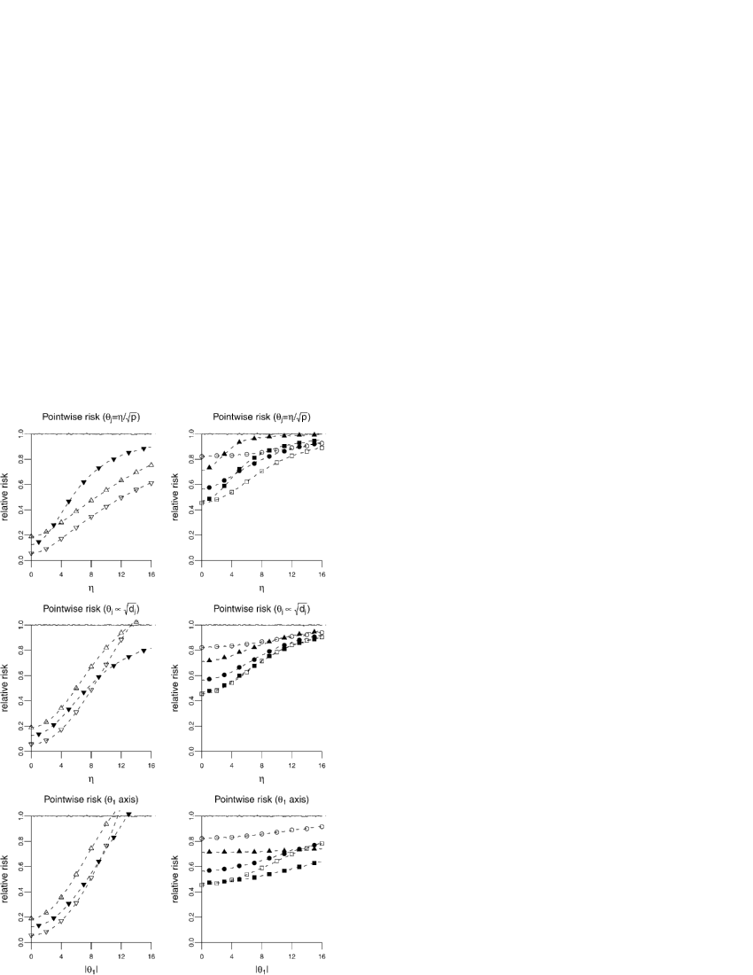
Figure 1: Pointwise risks along the homoscedastic (first row) and heteroscedastic (second row) directions and $\theta_{1}$ axis (third row) in the case (37). Left: non-minimax estimators $\delta^{\mathrm{EB}}$ ($\triangledown$), $\delta^{\mathrm{RB}}$ ($\blacktriangledown$), $\delta^{\mathrm{XKB}}$ ($\vartriangle$). Right: minimax estimators $\delta_{p-2}^{\mathrm{B}+}$ ($\blacktriangle$), $\delta^{\mathrm{MB}}$ with $\Gamma=0$ ($\bullet$) and $\Gamma=(16^{2}/p)I$ ($\circ$), $\delta^{+}_{A}$ with $A=A^{\dagger}_{0}$ ($\blacksquare$) and $A^{\dagger}_{\infty}$ ($\square$).

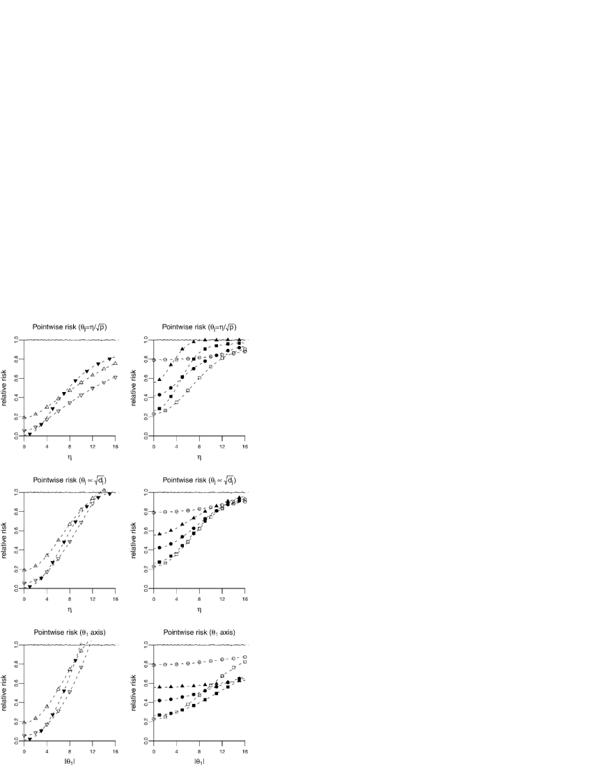
Figure 2: Pointwise risks along the homoscedastic (first row) and heteroscedastic (second row) directions and $\theta_{1}$ axis (third row) in the case (37), with the same legend as in Figure 1. The alternative versions of $\delta^{\mathrm{B}+}_{p-2}$, $\delta^{\mathrm{RB}}$, $\delta^{\mathrm{MB}}$, and $\delta^{+}_{A}$ are used.

4.2 Results

The relative performances of the estimators are found to be consistent across different configurations of $D$ studied. Moreover, the Bayes risk curves under the homoscedastic prior are similar to the pointwise risk curves along the homoscedastic direction. The Bayes risk curves under the heteroscedastic prior are similar to the pointwise risk curves along the heteroscedastic direction. Figure 1 shows the pointwise risks of the estimators with the usual versions of $\delta^{\mathrm{B}+}_{p-2}$, $\delta^{\mathrm{RB}}$, $\delta^{\mathrm{MB}}$, and $\delta^{+}_{A}$ and Figure 2 shows those of the estimators with the alternative versions of $\delta^{\mathrm{B}+}_{p-2}$, $\delta^{\mathrm{RB}}$, $\delta^{\mathrm{MB}}$, and $\delta^{+}_{A}$ for the case (37), with roughly three groups of coordinate variances, which might be considered unfavorable to our approach. For both $A^{\dagger}_{0}$ and $A^{\dagger}_{\infty}$, the cutoff index $\nu$ is found to be 3. See the supplementary material (Tan [30]) for the Bayes risk curves of all these estimators for the case (37) and the results for other configurations of $D$.

A number of observations can be drawn from Figures 1–2. First, $\delta^{\mathrm{EB}}$, $\delta^{\mathrm{XKB}}$, and $\delta^{\mathrm{RB}}$ have among the lowest risk curves along the homoscedastic direction. But along the heteroscedastic direction, the risk curves of $\delta^{\mathrm{EB}}$ and $\delta^{\mathrm{XKB}}$ rise quickly above the constant risk of $X$ as $\eta$ increases. Moreover, all the risk curves of $\delta^{\mathrm{EB}}$, $\delta^{\mathrm{XKB}}$, and $\delta^{\mathrm{RB}}$ along the $\theta_{1}$ axis exceed the constant risk of $X$ as $|\theta_{1}|$ increases. Therefore, $\delta^{\mathrm{EB}}$, $\delta^{\mathrm{XKB}}$, and $\delta^{\mathrm{RB}}$ fail to be minimax, as mentioned in Section 2.

Second, $\delta_{p-2}^{\mathrm{B}+}$ or $\delta_{2(p-2)}^{\mathrm{B}+}$ has among the highest risk curve, except where the risk curves of $\delta^{\mathrm{EB}}$ and $\delta^{\mathrm{XKB}}$ exceed the constant risk of $X$ along the heteroscedastic direction. The poor performance is expected for $\delta_{p-2}^{\mathrm{B}+}$ or $\delta_{2(p-2)}^{\mathrm{B}+}$, because there are considerable differences between the coordinate variances in (37).

Third, among the minimax estimators, $\delta^{+}_{A}$ with $A=A^{\dagger}_{0}$ or $A^{\dagger}_{\infty}$ has the lowest risk curve along various directions, whether the usual versions of $\delta^{\mathrm{B}+}_{p-2}$, $\delta^{\mathrm{MB}}$, and $\delta^{+}_{A}$ are compared (Figure 1) or the alternative versions are compared (Figure 2).

Fourth, the risk curve of $\delta^{+}_{A}$ with $A=A^{\dagger}_{0}$ is similar to that of $\delta^{+}_{A}$ with $A=A^{\dagger}_{\infty}$ along the heteroscedastic direction. But the former is noticeably higher than the latter along the homoscedastic direction as $\eta$ increases, whereas is noticeably lower than the latter along the $\theta_{1}$ axis as $|\theta_{1}|$ increases. These results agree with the construction of $A^{\dagger}_{0}$ using a heteroscedastic prior and $A^{\dagger}_{\infty}$ using a flat, homoscedastic prior. Their relative performances depend on the direction in which the risks are evaluated.

Fifth, $\delta^{\mathrm{MB}}$ with $\Gamma=0$ has risk curves below that of $\delta_{p-2}^{\mathrm{B}+}$ or $\delta_{2(p-2)}^{\mathrm{B}+}$, but either above or crossing those of $\delta^{+}_{A}$ with $A=A^{\dagger}_{0}$ and $A^{\dagger}_{\infty}$. Moreover, $\delta^{\mathrm{MB}}$ with $\Gamma=(16^{2}/p)I$ has elevated, almost flat risk curves for $\eta$ from 0 to 16. This seems to indicate an undesirable consequence of using a non-degenerate prior for $\delta^{\mathrm{MB}}$ in that the risk tends to increase for $\theta$ near 0, and remains high for $\theta$ far away from 0.

The foregoing discussion involves the comparison of the risk curves as $\theta$ moves away from 0 between $\delta^{\mathrm{MB}}$ and $\delta_{A^{\dagger}}^{+}$ specified with fixed priors. Alternatively, we compare the pointwise risks at $\theta=(\eta/\sqrt{p},\ldots,\eta/\sqrt{p})$ or $(\eta\sqrt{d_{1}},\ldots,\eta\sqrt{d_{p}})/\sqrt{\operatorname{tr}(D)}$ and the Bayes risks under the prior $\mathrm{N}(0,\eta^{2}I/p)$ or $\mathrm{N}\{0,\eta^{2}D/\operatorname{tr}(D)\}$ between $\delta^{\mathrm{MB}}$ and $\delta_{A^{\dagger}}^{+}$ specified with the prior $\mathrm{N}(0,\eta^{2}I/p)$ for a range of $\eta$. The homoscedastic prior used in the specification of $\delta^{\mathrm{MB}}$ and $\delta_{A^{\dagger}}^{+}$ can be considered correctly specified or misspecified, when the Bayes risks are evaluated under, respectively, the homoscedastic or heteroscedastic prior or when the pointwise risks are evaluated along the homoscedastic or heteroscedastic direction. For each situation, $\delta_{A^{\dagger}}^{+}$ has lower pointwise or Bayes risks than $\delta^{\mathrm{MB}}$. See Figure A2 in the supplementary material (Tan [30]).

5 Conclusion

The estimator $\delta_{A^{\dagger}}$ and its positive-part version $\delta^{+}_{A^{\dagger}}$ are not only minimax and but also have desirable properties including simplicity, interpretability, and effectiveness in risk reduction. In fact, $\delta_{A^{\dagger}}$ is defined by taking $A=A^{\dagger}$ in a class of minimax estimators $\delta_{A}$. The simplicity of $\delta_{A^{\dagger}}$ holds because $\delta_{A}$ is of the linear form $(I-\lambda A)X$, with $A$ and $\lambda$ indicating the direction and magnitude of shrinkage. The interpretability of $\delta_{A^{\dagger}}$ holds because the form of $A^{\dagger}$ indicates that one group of coordinates are shrunk in the direction of Berger’s [3] minimax estimator whereas the remaining coordinates are shrunk in the direction of the Bayes rule. The effectiveness of $\delta_{A^{\dagger}}$ in risk reduction is supported, in theory, by showing that $\delta_{A^{\dagger}}$ can achieve close to the minimum Bayes risk simultaneously over a scale class of normal priors (Corollary 4). For various scenarios in our numerical study, the estimators $\delta_{A^{\dagger}}^{+}$ with extreme priors yield more substantial risk reduction than existing minimax estimators.

It is interesting to discuss a special feature of $\delta_{A,r}$ and hence of $\delta_{A,c}$ and $\delta_{A}$ among linear, shrinkage estimators of the form

$$\delta=X-h\bigl{(}X^{\mathrm{T}}BX\bigr{)}AX,$$ (39)

where $A$ and $B$ are nonnegative definite matrices and $h(\cdot)$ is a scalar function. The estimator $\delta_{A,r}$ corresponds to the choice $B\propto A^{\mathrm{T}}QA$, which is motivated by the form of the optimal $\lambda$ in minimizing the risk of $(I-\lambda A)X$ for fixed $A$. On the other hand, Berger and Srinivasan [8] showed that under certain regularity conditions on $h(\cdot)$, an estimator (39) can be generalized Bayes or admissible only if $B\propto\Sigma^{-1}A$. This condition is incompatible with $B\propto A^{\mathrm{T}}QA$, unless $A\propto Q^{-1}\Sigma^{-1}$ as in Berger’s [3] estimator. Therefore, $\delta_{A}$ including $\delta_{A^{\dagger}}$ is, in general, not generalized Bayes or admissible. This conclusion, however, does not apply directly to the positive-part estimator $\delta_{A}^{+}$, which is no longer of the linear form $(I-\lambda A)X$.

There are various topics that can be further studied. First, the prior on $\theta$ is fixed, independently of data in the current paper. A useful extension is to allow the prior to be estimated within a certain class, for example, homoscedastic priors $N(0,\gamma I)$, from the data, in the spirit of empirical Bayes estimation (e.g., Efron and Morris [17]). Second, the Bayes risk with a normal prior is used to measure average risk reduction in an elliptical region (Section 3.3). It is interesting to study how our approach can be extended when using a non-normal prior on $\theta$, corresponding to a non-elliptical region in which risk reduction is desired.

Appendix

The following extends Stein’s [27] lemma for computing the expectation of the inner product of $X-\theta$ and a vector of functions of $X$.

Lemma 1

Let $X=(X_{1},\ldots,X_{p})^{\mathrm{T}}$ be multivariate normal with mean $\theta$ and variance matrix $\Sigma$. Assume that $g=(g_{1},\ldots,g_{p})^{\mathrm{T}}\mathchoice{\nobreak\,\colon}{\nobreak\,\colon}{\nobreak\,\colon\;}{\nobreak\,\colon\;}\mathcal{R}^{p}\to\mathcal{R}^{p}$ is almost differentiable Stein [27] with $E_{\theta}\{|\nabla_{j}g_{i}(X)|\}<\infty$ for $i,j=1,\ldots,p$, where $\nabla_{j}=\partial/\partial x_{j}$. Then

$$E_{\theta}\bigl{\{}(X-\theta)^{\mathrm{T}}g(X)\bigr{\}}=\operatorname{tr}\bigl{[}\Sigma E_{\theta}\bigl{\{}\nabla g(X)\bigr{\}}\bigr{]},$$

where $\nabla g(x)$ is the matrix with $(i,j)$th element $\nabla_{j}g_{i}(x)$.

Proof.

A direct generalization of Lemma 2 in Stein [27] to a normal random vector with non-identity variance matrix gives

$$E_{\theta}\bigl{\{}(X-\theta)g_{i}(X)\bigr{\}}=\Sigma E_{\theta}^{\mathrm{T}}\bigl{\{}\nabla g_{i}(X)\bigr{\}},$$

where $\nabla g_{i}(x)$ is the row vector with $j$th element $\nabla_{j}g_{i}(x)$. Taking the $i$th element of both sides of the equation gives

$$E_{\theta}\bigl{\{}(X_{i}-\theta_{i})g_{i}(X)\bigr{\}}=\sum_{j=1}^{p}\sigma_{ij}E_{\theta}\bigl{\{}\nabla_{j}g_{i}(X)\bigr{\}},$$

where $\sigma_{ij}$ is the $(i,j)$th element of $\Sigma$. Summing both sides of the preceding equation over $i$ gives the desired result. ∎

Proof of Theorem 1 By direct calculation, the risk of $\delta_{A,r}$ is

$$R(\delta_{A,r},\theta)=\operatorname{tr}(\Sigma Q)+E_{\theta}\biggl{(}\frac{r^{2}}{X^{\mathrm{T}}A^{\mathrm{T}}QAX}\biggr{)}-2E_{\theta}\biggl{\{}(X-\theta)^{\mathrm{T}}\frac{rQAX}{X^{\mathrm{T}}A^{\mathrm{T}}QAX}\biggr{\}}.$$

By Lemma 1 and the fact that $\operatorname{tr}(\Sigma QAXX^{\mathrm{T}}A^{\mathrm{T}}QA)=X^{\mathrm{T}}A^{\mathrm{T}}QA\Sigma QAX$, the third term after the minus sign in $R(\delta_{A,r},\theta)$ is

$$2E_{\theta}\biggl{\{}r\frac{\operatorname{tr}(\Sigma QA)}{X^{\mathrm{T}}A^{\mathrm{T}}QAX}\biggr{\}}-4E_{\theta}\biggl{\{}r\frac{X^{\mathrm{T}}A^{\mathrm{T}}QA\Sigma QAX}{(X^{\mathrm{T}}A^{\mathrm{T}}QAX)^{2}}\biggr{\}}+4E_{\theta}\biggl{(}r^{\prime}\frac{X^{\mathrm{T}}A^{\mathrm{T}}QA\Sigma QAX}{X^{\mathrm{T}}A^{\mathrm{T}}QAX}\biggr{)}.$$

By condition (14), $A^{\mathrm{T}}QA\Sigma QA$ is nonnegative definite. By Section 21.14 and Exercise 21.32 in Harville [18], $(x^{\mathrm{T}}A^{\mathrm{T}}QA\Sigma QAx)/(x^{\mathrm{T}}A^{\mathrm{T}}QAx)\leq\lambda_{\max}(A\Sigma Q+\Sigma A^{\mathrm{T}}Q)/2$ for $x\neq 0$. Then the preceding expression is bounded from below by

$$2E_{\theta}\biggl{\{}r\frac{\operatorname{tr}(\Sigma QA)-\lambda_{\max}(A\Sigma Q+\Sigma A^{\mathrm{T}}Q)}{X^{\mathrm{T}}A^{\mathrm{T}}QAX}\biggr{\}},$$

which leads immediately to the upper bound on $R(\delta_{A,r},\theta)$. Proof for condition (17) We show that if condition (17) holds, then there exists a nonsingular matrix $B$ with the claimed properties. The converse is trivially true. Let $R$ be the unique symmetric, positive definite matrix such that $R^{2}=Q$. Then $RAR^{-1}$ is symmetric, that is, $RAR^{-1}=R^{-1}A^{\mathrm{T}}R$, because $QA=A^{\mathrm{T}}Q$. Moreover, $R\Sigma R$ and $RAR^{-1}$ commute, that is, $RAR^{-1}(R\Sigma R)=R\Sigma R(RAR^{-1})^{\mathrm{T}}=R\Sigma R(RAR^{-1})$, because $A\Sigma=\Sigma A^{\mathrm{T}}$ and $RAR^{-1}$ is symmetric. Therefore, $R\Sigma R$ and $RAR^{-1}$ are simultaneously diagonalizable (Harville [18], Section 21.13). There exists an orthogonal matrix $O$ such that $O(R\Sigma R)O^{\mathrm{T}}=D$ and $O(RAR^{-1})O^{\mathrm{T}}=A^{*}$ for some diagonal matrices $D$ and $A^{*}$. Then $B=OR$ satisfies the claimed properties. Proof of inequality (20) We show that if $(Z_{1},\ldots,Z_{p})$ are independent standard normal variables, then $E\{(\sum_{j=1}^{p}a_{j}^{2}Z_{j}^{2})^{-1}\}\geq\{p/(p-2)\}(\sum_{j=1}^{p}a_{j}^{2})^{-1}$. Let $S=\sum_{j=1}^{p}Z_{j}^{2}$. Then $S$ and $(Z_{1}^{2}/S,\ldots,Z_{p}^{2}/S)$ are independent, $S\sim\chi^{2}_{p}$, and $(Z_{1}^{2}/S,\ldots,Z_{p}^{2}/S)\sim\operatorname{Dirichlet}(1/p,\ldots,1/p)$. The claimed inequality follows because $E\{(\sum_{j=1}^{p}a_{j}^{2}Z_{j}^{2})^{-1}\}=E\{(\sum_{j=1}^{p}a_{j}^{2}Z_{j}^{2}/S)^{-1}\}E(S^{-1})$, $E(S^{-1})=1/(p-2)$, and $E\{(\sum_{j=1}^{p}$ $a_{j}^{2}Z_{j}^{2}/S)^{-1}\}\geq\break(\sum_{j=1}^{p}a_{j}^{2}/p)^{-1}$ by Jensen’s inequality. Proofs of Theorem 2 and Corollary 2 Consider the transformation $\delta_{j}=d_{j}^{2}/(d_{j}+\gamma_{j})$ and $\alpha_{j}=\{(d_{j}+\gamma_{j})/d_{j}\}a_{j}$, so that $\delta_{j}\alpha_{j}=d_{j}a_{j}$ and $\delta_{j}\alpha_{j}^{2}=(d_{j}+\gamma_{j})a_{j}^{2}$. Problem (3.3) is then transformed to $\max_{\alpha_{1},\ldots,\alpha_{p}}\{\sum_{j=1}^{p}\delta_{j}\alpha_{j}-2\max(\delta_{1}\alpha_{1},\ldots,\delta_{p}\alpha_{p})\}$, subject to $\alpha_{j}\geq 0$ ($j=1,\ldots,p$) and $\sum_{j=1}^{p}\delta_{j}\alpha_{j}^{2}=\sum_{j=1}^{p}\delta_{j}$, which is of the form of the special case of (3.3) with $\gamma_{j}=0$ ($j=1,\ldots,p$). But it is easy to verify that if the claimed results hold for the transformed problem, then the results hold for original problem (3.3). Therefore, assume in the rest of proof that $\gamma_{j}=0$ ($j=1,\ldots,p$).

There exists at least a solution, $A^{\dagger}$, to problem (3.3) by boundedness of the constraint set. Let $\mathcal{K}=\{k\colon\ d_{k}a^{\dagger}_{k}=d_{\nu}a^{\dagger}_{\nu},k=1,\ldots,p\}$ and $\mathcal{K}^{c}=\{j\colon\ d_{j}a^{\dagger}_{j}<d_{\nu}a^{\dagger}_{\nu},j=1,\ldots,p\}$. A key of the proof is to exploit the fact that, by the setup of problem (3.3), $(a_{1}^{\dagger},\ldots,a_{p}^{\dagger})$ is automatically a solution to the problem

$$\max_{a_{1},\ldots,a_{p}}\quad\sum_{j=1}^{p}d_{j}a_{j}-2d_{\nu}a_{\nu},$$

$$\quad\mbox{subject to}\quad a_{j}\geq 0,\qquad d_{j}a_{j}\leq d_{\nu}a_{\nu}\qquad(j=1,\ldots,p),\quad\mbox{and}$$ (1)

$$\hphantom{\quad\mbox{subject to}\quad}\sum_{j=1}^{p}d_{j}a_{j}^{2}=\sum_{j=1}^{p}d_{j}.$$

The Karush–Kuhn–Tucker condition for this problem gives

$$-1+2\lambda a_{j}^{\dagger}-d_{j}^{-1}\rho_{j} = 0\qquad\mbox{for}j\in\mathcal{K}^{c},$$ (2)

$$-1+2\lambda a_{k}^{\dagger}+\mu_{k}-d_{k}^{-1}\rho_{k} = 0\qquad\mbox{for }k\ (\neq\nu)\in\mathcal{K},$$ (3)

$$-1+2\lambda a_{\nu}^{\dagger}+\biggl{(}2-\sum_{k\in\mathcal{K}\setminus\{\nu\}}\mu_{k}\biggr{)}-d_{\nu}^{-1}\rho_{\nu} = 0,$$ (4)

where $\lambda$, $\mu_{k}\geq 0$ ($k\in\mathcal{K}\setminus\{\nu\}$), and $\rho_{j}\geq 0$ satisfying $\rho_{j}a_{j}^{\dagger}=0$ ($j=1,\ldots,p$) are Lagrange multipliers.

First, we show that $a_{j}^{\dagger}>0$ and hence $\rho_{j}=0$ for $j=1,\ldots,p$. If $\mathcal{K}^{c}=\varnothing$, then either $a_{j}^{\dagger}>0$ for $j=1,\ldots,p$, or $a_{1}^{\dagger}=\cdots=a_{p}^{\dagger}=0$. The latter case is infeasible by the constraint $\sum_{j=1}^{p}d_{j}a_{j}^{2}=\sum_{j=1}^{p}d_{j}$. Suppose $\mathcal{K}^{c}\neq\varnothing$. By (2), $a_{j}^{\dagger}>0$ for each $j\in\mathcal{K}^{c}$. Then $a_{k}^{\dagger}>0$ for each $k\in\mathcal{K}$ because $d_{k}a_{k}^{\dagger}>d_{j}a_{j}^{\dagger}$.

Second, we show that $\nu\geq 3$. If $\mathcal{K}^{c}=\varnothing$, then $\nu=p\geq 3$. Suppose $\mathcal{K}^{c}\neq\varnothing$. Then $\lambda>0$ by (2). Summing (3) over $k\ (\neq\nu)\in\mathcal{K}$ and (4) shows that $-\nu+2\lambda\sum_{k=1}^{\nu}a_{k}^{\dagger}+2=0$. Therefore, $\nu>2$ or equivalently $\nu\geq 3$.

Third, we show that $\mathcal{K}=\{1,2,\ldots,\nu\}$ and $\mathcal{K}^{c}=\{\nu+1,\ldots,p\}$. For each $k\ (\neq\nu)\in\mathcal{K}$ and $j\in\mathcal{K}^{c}$, $a_{k}^{\dagger}\leq a_{j}^{\dagger}$ by (2)–(3) and then $d_{k}>d_{j}$ because $d_{k}a_{k}^{\dagger}>d_{j}a_{j}^{\dagger}$. The inequalities also hold for $k=\nu$, by application of the argument to problem (Appendix) with $\nu$ replaced by some $k\ (\neq\nu)\in\mathcal{K}$. Then $\mathcal{K}^{c}=\{\nu+1,\ldots,p\}$ because $d_{\nu}>d_{j}$ for each $j\in\mathcal{K}^{c}$, $d_{1}\geq d_{2}\geq\cdots\geq d_{p}$, and $\nu$ is the largest element in $\mathcal{K}$.

Fourth, we show the expressions for $(a_{1}^{\dagger},\ldots,a_{p}^{\dagger})$ and the achieved maximum value. By the definition of $\mathcal{K}$, $a_{k}^{\dagger}\propto d_{k}^{-1}$ for $k=1,\ldots,\nu$. By (2), $a_{j}^{\dagger}\propto 1$ for $j=\nu+1,\ldots,p$. Let $y^{\dagger}=d_{\nu}a^{\dagger}_{\nu}$ and $z^{\dagger}=a^{\dagger}_{\nu+1}$. Then $(y^{\dagger},z^{\dagger})$ is a solution to the problem

$$\max_{y,z}\quad(\nu-2)y+\Biggl{(}\sum_{j=\nu+1}^{p}d_{j}\Biggr{)}z,$$

$$\quad\mbox{subject to}\quad y\geq 0,\qquad z\geq 0,\qquad y\geq d_{\nu+1}z,\quad\mbox{and}$$

$$\hphantom{\quad\mbox{subject to}\quad}\Biggl{(}\sum_{k=1}^{\nu}d_{k}^{-1}\Biggr{)}y^{2}+\Biggl{(}\sum_{j=\nu+1}^{p}d_{j}\Biggr{)}z^{2}=\sum_{j=1}^{p}d_{j}.$$

By the definition of $\mathcal{K}$, $y^{\dagger}>d_{\nu+1}z^{\dagger}$ and hence $(y^{\dagger},z^{\dagger})$ lies off the boundary in the constraint set. Then $(y^{\dagger},z^{\dagger})$ is a solution to the foregoing problem with the constraint $y\geq d_{\nu+1}z$ removed. The problem is of the form of maximizing a linear function of $(y,z)$ subject to an elliptical constraint. Straightforward calculation shows that

$$y^{\dagger}=\biggl{(}\frac{\sum_{j=1}^{p}d_{j}}{M_{\nu}}\biggr{)}^{1/2}\frac{\nu-2}{\sum_{j=1}^{\nu}d_{j}^{-1}},\qquad z^{\dagger}=\biggl{(}\frac{\sum_{j=1}^{p}d_{j}}{M_{\nu}}\biggr{)}^{1/2},$$

and the achieved maximum value is $(\sum_{j=1}^{p}d_{j})^{1/2}M_{\nu}^{1/2}$, where $M_{\nu}=(\nu-2)^{2}/(\sum_{j=1}^{\nu}d_{j}^{-1})$ $+\sum_{j=\nu+1}^{p}d_{j}$ .

Finally, we show that the sequence $(M_{3},M_{4},\ldots M_{p})$ is nonincreasing: $M_{k}\geq M_{k+1}$, where the equality holds if and only if $k-2=\sum_{j=1}^{k}d_{k+1}/d_{j}$. Because $y^{\dagger}>d_{\nu+1}z^{\dagger}$ or $\nu-2>\sum_{j=1}^{\nu}d_{\nu+1}/d_{j}$, this result implies that $M_{\nu}>M_{\nu+1}$ and hence $A^{\dagger}$ is a unique solution to (3.3). Let $L_{k}=\{(\sum_{j=1}^{k}d_{j})(\sum_{j=1}^{k}d_{j}^{-1})-(k-2)^{2}\}/\sum_{j=1}^{k}d_{j}^{-1}$ so that $M_{k}=\sum_{j=1}^{p}d_{j}-L_{k}$. By the identity $(b+\beta)/(a+\alpha)-b/a=(\beta/\alpha-b/a)\{\alpha/(a+\alpha)\}$ and simple calculation,

$$L_{k+1}-L_{k} = \Biggl{[}\frac{\sum_{j=1}^{k}(d_{j}/d_{k+1}+d_{k+1}/d_{j})-2k+4}{d_{k+1}^{-1}}-\Biggl{\{}\sum_{j=1}^{k}d_{j}-\frac{(k-2)^{2}}{\sum_{j=1}^{k}d_{j}^{-1}}\Biggr{\}}\Biggr{]}\frac{d_{k+1}^{-1}}{\sum_{j=1}^{k+1}d_{j}^{-1}}$$

$$= d_{k+1}\frac{\{r_{k}-(k-2)\}^{2}}{r_{k}(r_{k}+1)},$$

where $r_{k}=\sum_{j=1}^{k}d_{k+1}/d_{j}$. Therefore, $L_{k}\leq L_{k+1}$. Moreover, $L_{k}=L_{k+1}$ if and only if $r_{k}=k-2$, that is, $\sum_{j=1}^{k}d_{k+1}/d_{j}=k-2$. Proof of Corollary 3 It suffices to show (25). By Corollary 2, $\sum_{k=1}^{\nu-1}d_{\nu}^{*}/d_{k}^{*}\geq\nu-3$ and hence $\sum_{k=1}^{\nu}d_{\nu}^{*}/d_{k}^{*}\geq\nu-2$. Then for $j=1,\ldots,\nu$.

$$a_{j}^{\dagger}=\frac{(\nu-2){d_{j}^{*}}^{-1}}{\sum_{k=1}^{\nu}{d_{k}^{*}}^{-1}}\frac{d_{j}}{d_{j}+\gamma_{j}}\leq\frac{(\nu-2){d_{\nu}^{*}}^{-1}}{\sum_{k=1}^{\nu}{d_{k}^{*}}^{-1}}\frac{d_{j}}{d_{j}+\gamma_{j}}\leq\frac{d_{j}}{d_{j}+\gamma_{j}},$$

because $d_{j}^{*}\geq d_{\nu}^{*}$ for $j\leq\nu$. Proof of Theorem 3 Let $L_{k}=\sum_{j=1}^{k}d_{j}^{*}-(k-2)^{2}/\sum_{j=1}^{k}{d_{j}^{*}}^{-1}$ so that $M_{k}=\sum_{j=1}^{p}d_{j}^{*}-L_{k}$, similarly as in the proof of Theorem 2. By equation (Appendix) with $r_{k}=\sum_{j=1}^{k}d_{k+1}^{*}/d_{j}^{*}$ and $d_{k+1}$ replaced by $d_{k+1}^{*}$,

$$L_{\nu}=L_{3}+\sum_{k=3}^{\nu-1}(L_{k+1}-L_{k})=L_{3}+\sum_{k=3}^{\nu-1}d_{k+1}^{*}\frac{\{r_{k}-(k-2)\}^{2}}{r_{k}(r_{k}+1)}.$$

By the relationship $r_{k}=(d_{k+1}^{*}/d_{k}^{*})(1+r_{k-1})$ and simple calculation,

$$L_{3} = d_{1}^{*}+d_{2}^{*}+d_{3}^{*}-\frac{1}{{d_{1}^{*}}^{-1}+{d_{2}^{*}}^{-1}+{d_{3}^{*}}^{-1}}$$

$$= d_{1}^{*}+d_{2}^{*}+d_{3}^{*}-\sum_{k=3}^{\nu-1}d_{k+1}^{*}\biggl{(}\frac{1}{r_{k}}-\frac{1}{r_{k}+1}\biggr{)}-\frac{d_{\nu}^{*}}{r_{\nu-1}+1}.$$

If $\nu\geq 4$, combining the two preceding equation gives

$$L_{\nu} = d_{1}^{*}+d_{2}^{*}+d_{3}^{*}+\sum_{k=3}^{\nu-1}d_{k+1}^{*}\frac{\{r_{k}-(k-2)\}^{2}-1}{r_{k}(r_{k}+1)}-\frac{d_{\nu}^{*}}{r_{\nu-1}+1}$$

$$\leq d_{1}^{*}+d_{2}^{*}+d_{3}^{*}+\sum_{k=3}^{\nu-1}d_{k+1}^{*}\frac{3}{k(k+1)}-\frac{d_{\nu}^{*}}{\nu}$$

$$= d_{1}^{*}+d_{2}^{*}+d_{3}^{*}+d_{4}^{*}-3\sum_{k=3}^{\nu-2}\frac{d_{k+1}^{*}-d_{k+2}^{*}}{k+1}-4\frac{d_{\nu}^{*}}{\nu}$$

$$\leq d_{1}^{*}+d_{2}^{*}+d_{3}^{*}+d_{4}^{*}-4\frac{d_{\nu}^{*}}{\nu}.$$

The first inequality follows because $k-2\leq r_{k}\leq k$ for $k=3,\ldots,\nu-1$ and $\{t-(k-2)\}^{2}/\{t(t+1)\}$ is increasing for $k-2\leq t\leq k$ with a maximum at $t=k$. The second inequality follows because $d_{1}^{*}\geq d_{2}^{*}\geq\cdots\geq d_{p}^{*}$. Therefore, if $\nu\geq 4$ then

$$\frac{p}{p-2}M_{\nu} \geq \frac{p}{p-2}\Biggl{\{}\sum_{j=1}^{p}d_{j}^{*}-\biggl{(}d_{1}^{*}+d_{2}^{*}+d_{3}^{*}+d_{4}^{*}-4\frac{d_{\nu}^{*}}{\nu}\biggr{)}\Biggr{\}}$$

$$= \sum_{j=3}^{p}d_{j}^{*}-\Biggl{(}d_{3}^{*}+d_{4}^{*}-\frac{2}{p-2}\sum_{j=5}^{p}d_{j}^{*}-\frac{4p}{p-2}\frac{d_{\nu}^{*}}{\nu}\Biggr{)}.$$

If $\nu=3$, then $L_{\nu}\leq d_{1}^{*}+d_{2}^{*}+d_{3}^{*}-d_{3}^{*}/3$ and hence

$$\frac{p}{p-2}M_{\nu} \geq \frac{p}{p-2}\Biggl{\{}\sum_{j=1}^{p}d_{j}^{*}-\bigl{(}d_{1}^{*}+d_{2}^{*}+d_{3}^{*}-d_{3}^{*}/3\bigr{)}\Biggr{\}}$$

$$= \sum_{j=3}^{p}d_{j}^{*}-\Biggl{(}d_{3}^{*}-\frac{2}{p-2}\sum_{j=4}^{p}d_{j}^{*}-\frac{p}{p-2}\frac{d_{3}^{*}}{3}\Biggr{)}.$$

This completes the proof.

References

• [1] {bmisc}[mr] \bauthor\bsnmBaranchik, \bfnmAlvin John\binitsA.J. (\byear1964). \bhowpublishedMultiple regression and estimation of the mean of a multivariate normal distribution. Technical Report 51, Dept. Statistics, Stanford Univ. \bptokimsref\endbibitem
• [2] {barticle}[mr] \bauthor\bsnmBaranchik, \bfnmA. J.\binitsA.J. (\byear1970). \btitleA family of minimax estimators of the mean of a multivariate normal distribution. \bjournalAnn. Math. Statist. \bvolume41 \bpages642–645. \bidissn=0003-4851, mr=0253461 \bptokimsref\endbibitem
• [3] {barticle}[mr] \bauthor\bsnmBerger, \bfnmJames O.\binitsJ.O. (\byear1976). \btitleAdmissible minimax estimation of a multivariate normal mean with arbitrary quadratic loss. \bjournalAnn. Statist. \bvolume4 \bpages223–226. \bidissn=0090-5364, mr=0397940 \bptokimsref\endbibitem
• [4] {barticle}[mr] \bauthor\bsnmBerger, \bfnmJames\binitsJ. (\byear1980). \btitleA robust generalized Bayes estimator and confidence region for a multivariate normal mean. \bjournalAnn. Statist. \bvolume8 \bpages716–761. \bidissn=0090-5364, mr=0572619 \bptokimsref\endbibitem
• [5] {barticle}[mr] \bauthor\bsnmBerger, \bfnmJames O.\binitsJ.O. (\byear1982). \btitleSelecting a minimax estimator of a multivariate normal mean. \bjournalAnn. Statist. \bvolume10 \bpages81–92. \bidissn=0090-5364, mr=0642720 \bptokimsref\endbibitem
• [6] {bbook}[mr] \bauthor\bsnmBerger, \bfnmJames O.\binitsJ.O. (\byear1985). \btitleStatistical Decision Theory and Bayesian Analysis, \bedition2nd ed. \bseriesSpringer Series in Statistics. \blocationNew York: \bpublisherSpringer. \bidmr=0804611 \bptokimsref\endbibitem
• [7] {barticle}[mr] \bauthor\bsnmBerger, \bfnmJames O.\binitsJ.O. &\bauthor\bsnmRobert, \bfnmChristian\binitsC. (\byear1990). \btitleSubjective hierarchical Bayes estimation of a multivariate normal mean: On the frequentist interface. \bjournalAnn. Statist. \bvolume18 \bpages617–651. \biddoi=10.1214/aos/1176347619, issn=0090-5364, mr=1056330 \bptokimsref\endbibitem
• [8] {barticle}[mr] \bauthor\bsnmBerger, \bfnmJames O.\binitsJ.O. &\bauthor\bsnmSrinivasan, \bfnmC.\binitsC. (\byear1978). \btitleGeneralized Bayes estimators in multivariate problems. \bjournalAnn. Statist. \bvolume6 \bpages783–801. \bidissn=0090-5364, mr=0478426 \bptokimsref\endbibitem
• [9] {barticle}[mr] \bauthor\bsnmBhattacharya, \bfnmP. K.\binitsP.K. (\byear1966). \btitleEstimating the mean of a multivariate normal population with general quadratic loss function. \bjournalAnn. Math. Statist. \bvolume37 \bpages1819–1824. \bidissn=0003-4851, mr=0201026 \bptokimsref\endbibitem
• [10] {barticle}[mr] \bauthor\bsnmBock, \bfnmM. E.\binitsM.E. (\byear1975). \btitleMinimax estimators of the mean of a multivariate normal distribution. \bjournalAnn. Statist. \bvolume3 \bpages209–218. \bidissn=0090-5364, mr=0381064 \bptokimsref\endbibitem
• [11] {barticle}[mr] \bauthor\bsnmBrandwein, \bfnmAnn Cohen\binitsA.C. &\bauthor\bsnmStrawderman, \bfnmWilliam E.\binitsW.E. (\byear1990). \btitleStein estimation: The spherically symmetric case. \bjournalStatist. Sci. \bvolume5 \bpages356–369. \bidissn=0883-4237, mr=1080957 \bptokimsref\endbibitem
• [12] {barticle}[mr] \bauthor\bsnmBrown, \bfnmLawrence D.\binitsL.D. (\byear1975). \btitleEstimation with incompletely specified loss functions (the case of several location parameters). \bjournalJ. Amer. Statist. Assoc. \bvolume70 \bpages417–427. \bidissn=0162-1459, mr=0373082 \bptokimsref\endbibitem
• [13] {barticle}[mr] \bauthor\bsnmBrown, \bfnmLawrence D.\binitsL.D. &\bauthor\bsnmZhao, \bfnmLinda H.\binitsL.H. (\byear2009). \btitleEstimators for Gaussian models having a block-wise structure. \bjournalStatist. Sinica \bvolume19 \bpages885–903. \bidissn=1017-0405, mr=2536135 \bptokimsref\endbibitem
• [14] {barticle}[mr] \bauthor\bsnmCai, \bfnmT. Tony\binitsT.T. (\byear2012). \btitleMinimax and adaptive inference in nonparametric function estimation. \bjournalStatist. Sci. \bvolume27 \bpages31–50. \biddoi=10.1214/11-STS355, issn=0883-4237, mr=2953494 \bptokimsref\endbibitem
• [15] {barticle}[mr] \bauthor\bsnmCasella, \bfnmGeorge\binitsG. (\byear1985). \btitleCondition numbers and minimax ridge regression estimators. \bjournalJ. Amer. Statist. Assoc. \bvolume80 \bpages753–758. \bidissn=0162-1459, mr=0803264 \bptokimsref\endbibitem
• [16] {barticle}[mr] \bauthor\bsnmDonoho, \bfnmDavid L.\binitsD.L., \bauthor\bsnmLiu, \bfnmRichard C.\binitsR.C. &\bauthor\bsnmMacGibbon, \bfnmBrenda\binitsB. (\byear1990). \btitleMinimax risk over hyperrectangles, and implications. \bjournalAnn. Statist. \bvolume18 \bpages1416–1437. \biddoi=10.1214/aos/1176347758, issn=0090-5364, mr=1062717 \bptokimsref\endbibitem
• [17] {barticle}[mr] \bauthor\bsnmEfron, \bfnmBradley\binitsB. &\bauthor\bsnmMorris, \bfnmCarl\binitsC. (\byear1973). \btitleStein’s estimation rule and its competitors—an empirical Bayes approach. \bjournalJ. Amer. Statist. Assoc. \bvolume68 \bpages117–130. \bidissn=0162-1459, mr=0388597 \bptokimsref\endbibitem
• [18] {bbook}[auto:STB—2014/01/06—10:16:28] \bauthor\bsnmHarville, \bfnmD. A.\binitsD.A. (\byear2008). \btitleMatrix Algebra from a Statistician’s Perspective. \blocationNew York: \bpublisherSpringer. \bptokimsref\endbibitem
• [19] {bincollection}[mr] \bauthor\bsnmJames, \bfnmW.\binitsW. &\bauthor\bsnmStein, \bfnmCharles\binitsC. (\byear1961). \btitleEstimation with quadratic loss. In \bbooktitleProc. 4th Berkeley Sympos. Math. Statist. and Prob., Vol. I \bpages361–379. \blocationBerkeley, CA: \bpublisherUniv. California Press. \bidmr=0133191 \bptokimsref\endbibitem
• [20] {barticle}[mr] \bauthor\bsnmJones, \bfnmM. C.\binitsM.C. (\byear1986). \btitleExpressions for inverse moments of positive quadratic forms in normal variables. \bjournalAustral. J. Statist. \bvolume28 \bpages242–250. \bidissn=0004-9581, mr=0860469 \bptokimsref\endbibitem
• [21] {bbook}[mr] \bauthor\bsnmLehmann, \bfnmE. L.\binitsE.L. &\bauthor\bsnmCasella, \bfnmGeorge\binitsG. (\byear1998). \btitleTheory of Point Estimation, \bedition2nd ed. \bseriesSpringer Texts in Statistics. \blocationNew York: \bpublisherSpringer. \bidmr=1639875 \bptokimsref\endbibitem
• [22] {barticle}[mr] \bauthor\bsnmMorris, \bfnmCarl N.\binitsC.N. (\byear1983). \btitleParametric empirical Bayes inference: Theory and applications. \bjournalJ. Amer. Statist. Assoc. \bvolume78 \bpages47–65. \bnoteWith discussion. \bidissn=0162-1459, mr=0696849 \bptokimsref\endbibitem
• [23] {barticle}[mr] \bauthor\bsnmMorris, \bfnmCarl N.\binitsC.N. &\bauthor\bsnmLysy, \bfnmMartin\binitsM. (\byear2012). \btitleShrinkage estimation in multilevel normal models. \bjournalStatist. Sci. \bvolume27 \bpages115–134. \biddoi=10.1214/11-STS363, issn=0883-4237, mr=2953499 \bptokimsref\endbibitem
• [24] {barticle}[pbm] \bauthor\bsnmSatterthwaite, \bfnmF. E.\binitsF.E. (\byear1946). \btitleAn approximate distribution of estimates of variance components. \bjournalBiometrics \bvolume2 \bpages110–114. \bidissn=0006-341X, pmid=20287815 \bptokimsref\endbibitem
• [25] {binproceedings}[mr] \bauthor\bsnmStein, \bfnmCharles\binitsC. (\byear1956). \btitleInadmissibility of the usual estimator for the mean of a multivariate normal distribution. In \bbooktitleProceedings of the Third Berkeley Symposium on Mathematical Statistics and Probability, 1954–1955, Vol. I \bpages197–206. \blocationBerkeley and Los Angeles: \bpublisherUniv. California Press. \bidmr=0084922 \bptokimsref\endbibitem
• [26] {barticle}[mr] \bauthor\bsnmStein, \bfnmC. M.\binitsC.M. (\byear1962). \btitleConfidence sets for the mean of a multivariate normal distribution. \bjournalJ. Roy. Statist. Soc. Ser. B \bvolume24 \bpages265–296. \bidissn=0035-9246, mr=0148184 \bptnotecheck related \bptokimsref\endbibitem
• [27] {barticle}[mr] \bauthor\bsnmStein, \bfnmCharles M.\binitsC.M. (\byear1981). \btitleEstimation of the mean of a multivariate normal distribution. \bjournalAnn. Statist. \bvolume9 \bpages1135–1151. \bidissn=0090-5364, mr=0630098 \bptokimsref\endbibitem
• [28] {barticle}[mr] \bauthor\bsnmStrawderman, \bfnmWilliam E.\binitsW.E. (\byear1971). \btitleProper Bayes minimax estimators of the multivariate normal mean. \bjournalAnn. Math. Statist. \bvolume42 \bpages385–388. \bidissn=0003-4851, mr=0397939 \bptokimsref\endbibitem
• [29] {binproceedings}[mr] \bauthor\bsnmStrawderman, \bfnmWilliam E.\binitsW.E. (\byear2010). \btitleBayesian decision based estimation and predictive inference. In \bbooktitleFrontiers of Statistical Decision Making and Bayesian Analysis: In Honor of James O. Berger (\beditorM.-H. Chen et al., eds.) \bpages69–82. \blocationNew York: \bpublisherSpringer. \bptokimsref\endbibitem
• [30] {bmisc}[auto:STB—2014/01/06—10:16:28] \bauthor\bsnmTan, \bfnmZ.\binitsZ. (\byear2014). \bhowpublishedSupplement to “Improved minimax estimation of a multivariate normal mean under heteroscedasticity”. DOI:\doiurl10.3150/13-BEJ580SUPP. \bptokimsref\endbibitem
• [31] {barticle}[mr] \bauthor\bsnmXie, \bfnmXianchao\binitsX., \bauthor\bsnmKou, \bfnmS. C.\binitsS.C. &\bauthor\bsnmBrown, \bfnmLawrence D.\binitsL.D. (\byear2012). \btitleSURE estimates for a heteroscedastic hierarchical model. \bjournalJ. Amer. Statist. Assoc. \bvolume107 \bpages1465–1479. \biddoi=10.1080/01621459.2012.728154, issn=0162-1459, mr=3036408 \bptokimsref\endbibitem