A Practical Guide to Randomized Matrix Computations with MATLAB Implementations

Abstract

Matrix operations such as matrix inversion, eigenvalue decomposition, singular value decomposition are ubiquitous in real-world applications. Unfortunately, many of these matrix operations so time and memory expensive that they are prohibitive when the scale of data is large. In real-world applications, since the data themselves are noisy, machine-precision matrix operations are not necessary at all, and one can sacrifice a reasonable amount of accuracy for computational efficiency.

In recent years, a bunch of randomized algorithms have been devised to make matrix computations more scalable. Mahoney [16] and Woodruff [34] have written excellent but very technical reviews of the randomized algorithms. Differently, the focus of this paper is on intuition, algorithm derivation, and implementation. This paper should be accessible to people with knowledge in elementary matrix algebra but unfamiliar with randomized matrix computations. The algorithms introduced in this paper are all summarized in a user-friendly way, and they can be implemented in lines of MATLAB code. The readers can easily follow the implementations even if they do not understand the maths and algorithms.

Keywords: matrix computation, randomized algorithms, matrix sketching, random projection, random selection, least squares regression, randomized SVD, matrix inversion, eigenvalue decomposition, kernel approximation, the Nyström method.

Chapter 1 Introduction

Matrix computation plays a key role in modern data science. However, matrix computations such as matrix inversion, eigenvalue decomposition, SVD, etc, are very time and memory expensive, which limits their scalability and applications. To make large-scale matrix computation possible, randomized matrix approximation techniques have been proposed and widely applied. Especially in the past decade, remarkable progresses in randomized numerical linear algebra has been made, and now large-scale matrix computations are no longer impossible tasks.

This paper reviews the most recent progresses of randomized matrix computation. The papers written by Mahoney [16] and Woodruff [34] provide comprehensive and rigorous reviews of the randomized matrix computation algorithms. However, their focus are on the theoretical properties and error analysis techniques, and readers unfamiliar with randomized numerical linear algebra can have difficulty when implementing their algorithms.

Differently, the focus of this paper is on intuitions and implementations, and the target readers are those who are familiar with basic matrix algebra but has little knowledge in randomized matrix computations. All the algorithms in this paper are described in a user-friend way. This paper also provides MATLAB implementations of the important algorithms. MATLAB code is easy to understand, easy to debug, and easy to translate to other languages. The users can even directly use the provided MATLAB code without understanding it.

This paper covers the following topics:

• Chapter 2 briefly reviews some matrix algebra preliminaries. This chapter can be skipped if the reader is familiar with matrix algebra.

• Chapter 3 introduces the techniques for generating a sketch of a large-scale matrix.

• Chapter 4 studies the least squares regression (LSR) problem where $n\gg d$.

• Chapter 5 studies efficient algorithms for computing the $k$-SVD of arbitrary matrices.

• Chapter 6 introduces techniques for sketching symmetric positive semi-definite (SPSD) matrices. The applications includes spectral clustering, kernel methods (e.g. Gaussian process regression and kernel PCA), and second-order optimization (e.g. Newton’s method).

Chapter 2 Elementary Matrix Algebra

This chapter defines the matrix notation and goes through the very basics of matrix decompositions. Particularly, the singular value decomposition (SVD), the QR decomposition, and the Moore-Penrose inverse are used throughout this paper.

2.1 Notation

Let ${\bf A}=[a_{ij}]$ be a matrix, ${\bf a}=[a_{i}]$ be a column vector, and $a$ be a scalar. The $i$-th row and $j$-th column of ${\bf A}$ are denoted by ${\bf a}_{i:}$ and ${\bf a}_{:j}$, respectively. When there is no ambiguity, either column or row can be written as ${\bf a}_{l}$. Let ${\bf I}_{n}$ be the $n\times n$ identity matrix, that is, the diagonal entries are ones and off-diagonal entries are zeros. The column space (the space spanned by the columns) of ${\bf A}$ is the set of all possible linear combinations of its column vectors. Let $[n]$ be the set $\{1,2,\cdots,n\}$. Let $\mathrm{nnz}({\bf A})$ be the number of nonzero entries of ${\bf A}$.

The squared vector $\ell_{2}$ norm is defined by

$$\|{\bf a}\|_{2}^{2}\;=\;{\sum_{i}a_{i}^{2}}.$$

The squared matrix Frobenius norm is defined by

$$\|{\bf A}\|_{F}\;=\;{\sum_{ij}a_{ij}^{2}},$$

and the matrix spectral norm is defined by

$$\|{\bf A}\|_{2}\;=\;\max_{{\bf x}\neq{\bf 0}}\frac{\|{\bf A}{\bf x}\|_{2}}{\|{\bf x}\|_{2}}.$$

2.2 Matrix Decompositions

QR decomposition. Let ${\bf A}$ be an $m\times n$ matrix with $m\geq n$. The QR decomposition of ${\bf A}$ is

$${\bf A}\;=\;\underbrace{{\bf Q}_{\bf A}}_{m\times n}\underbrace{{\bf R}_{\bf A}}_{n\times n}.$$

The matrix ${\bf Q}_{\bf A}$ has orthonormal columns, that is, ${\bf Q}_{{\bf A}}^{T}{\bf Q}_{{\bf A}}={\bf I}_{n}$. The matrix ${\bf R}_{\bf A}$ is upper triangular, that is, for all $i<j$, the $(i,j)$-th entry of ${\bf R}_{\bf A}$ is zero.

SVD. Let ${\bf A}$ be an $m\times n$ matrix and $\rho=\mathrm{rank}({\bf A})$. The condensed singular value decomposition (SVD) of ${\bf A}$ is

$$\underbrace{{\bf A}}_{m\times n}\;=\;\underbrace{{\bf U}_{\bf A}}_{m\times\rho}\underbrace{\mbox{\boldmath$\Sigma$\unboldmath}_{\bf A}}_{\rho\times\rho}\underbrace{{\bf V}_{\bf A}^{T}}_{\rho\times n}\;=\;\sum_{i=1}^{\rho}\sigma_{{\bf A},i}{\bf u}_{{\bf A},i}{\bf v}_{{\bf A},i}^{T}.$$

Here $\sigma_{{\bf A},1}\geq\cdots\geq\sigma_{{\bf A},\rho}>0$ are the singular values, ${\bf u}_{{\bf A},1},\cdots,{\bf u}_{{\bf A},\rho}\in{\mathbb{R}}^{m}$ are the left singular vectors, and ${\bf v}_{{\bf A},1},\cdots,{\bf v}_{{\bf A},\rho}\in{\mathbb{R}}^{n}$ are the right singular vectors. Unless otherwise specified, “SVD” refers to the condensed SVD.

$k$-SVD. In applications such as the principal component analysis (PCA), latent semantic indexing (LSI), word2vec, spectral clustering, we are only interested in the top $k$ ($\ll m,n$) singular values and singular vectors. The rank $k$ truncated SVD ($k$-SVD) is denoted by

$${\bf A}_{k}\;:=\;\sum_{i=1}^{k}\sigma_{{\bf A},i}{\bf u}_{{\bf A},i}{\bf v}_{{\bf A},i}^{T}\;=\;\underbrace{{\bf U}_{{\bf A},k}}_{m\times k}\underbrace{\mbox{\boldmath$\Sigma$\unboldmath}_{{\bf A},k}}_{k\times k}\underbrace{{\bf V}_{{\bf A},k}^{T}}_{k\times n}.$$

Here ${\bf U}_{{\bf A},k}$ consists of the first $k$ singular vectors of ${\bf U}_{\bf A}$, and $\mbox{\boldmath$\Sigma$\unboldmath}_{{\bf A},k}$ and ${\bf V}_{{\bf V},k}$ are analogously defined. Among all the $m\times n$ rank $k$ matrices, ${\bf A}_{k}$ is the closest approximation to ${\bf A}$ in that

$${\bf A}_{k}\;=\;\mathop{\rm argmin}_{{\bf X}}\|{\bf A}-{\bf X}\|_{F}^{2}\;=\;\mathop{\rm argmin}_{{\bf X}}\|{\bf A}-{\bf X}\|_{2}^{2},\qquad\mathsf{s.t.}\;\mathrm{rank}({\bf X})\leq k.$$

Eigenvalue decomposition. The eigenvalue decomposition of an $n\times n$ symmetric matrix ${\bf A}$ is defined by

$${\bf A}\;=\;{\bf U}_{\bf A}\mbox{\boldmath$\Lambda$\unboldmath}_{\bf A}{\bf U}_{\bf A}^{T}\;=\;\sum_{i=1}^{n}\lambda_{{\bf A},i}{\bf u}_{{\bf A},i}{\bf u}_{{\bf A},i}^{T}.$$

Here $\lambda_{{\bf A},1}\geq\cdots\geq\lambda_{{\bf A},n}$ are the eigenvalues of ${\bf A}$, and ${\bf u}_{{\bf A},1},\cdots,{\bf u}_{{\bf A},n}\in{\mathbb{R}}^{n}$ are the corresponding eigenvectors. A symmetric matrix ${\bf A}$ is called symmetric positive semidefinite (SPSD) if and only if all the eigenvalues are nonnegative. If ${\bf A}$ is SPSD, its SVD and eigenvalue decomposition are identical.

2.3 Matrix (Pseudo) Inverse and Orthogonal Projector

For an $n\times n$ square matrix ${\bf A}$, the matrix inverse exists if ${\bf A}$ is non-singular ($\mathrm{rank}({\bf A})=n$). Let ${\bf A}^{-1}$ be the inverse of ${\bf A}$. Then ${\bf A}{\bf A}^{-1}={\bf A}^{-1}{\bf A}={\bf I}_{n}$.

Only square and full rank matrices have inverse. For the general rectangular matrices or rank deficient matrices, matrix pseudo-inverse is used as a generalization of matrix inverse. The book [1] offers a comprehensive study of the pseudo-inverses.

The Moore-Penrose inverse is the most widely used pseudo-inverse, which is defined by

$${\bf A}^{\dagger}\;:=\;{\bf V}_{{\bf A}}\mbox{\boldmath$\Sigma$\unboldmath}_{\bf A}^{-1}{\bf U}_{{\bf A}}^{T}.$$

Let ${\bf A}$ be any $m\times n$ and rank $\rho$ matrix. Then

$${\bf A}{\bf A}^{\dagger}\;=\;{\bf U}_{{\bf A}}\mbox{\boldmath$\Sigma$\unboldmath}_{\bf A}\underbrace{{\bf V}_{{\bf A}}^{T}{\bf V}_{{\bf A}}}_{={\bf I}_{\rho}}\mbox{\boldmath$\Sigma$\unboldmath}_{\bf A}^{-1}{\bf U}_{{\bf A}}^{T}\;=\;\underbrace{{\bf U}_{{\bf A}}}_{m\times\rho}\underbrace{{\bf U}_{{\bf A}}^{T}}_{\rho\times m},$$

which is a orthogonal projector. It is because for any matrix ${\bf B}$, the matrix ${\bf A}{\bf A}^{\dagger}{\bf B}={\bf U}_{\bf A}{\bf U}_{\bf A}^{T}{\bf B}$ is the projection of ${\bf B}$ onto the column space of ${\bf A}$.

2.4 Time and Memory Costs

The time complexities of the matrix operations are listed in the following.

• Multiplying an $m\times n$ matrix ${\bf A}$ by an $n\times p$ matrix ${\bf B}$: ${\mathcal{O}}(mnp)$ float point operations (flops) in general, and ${\mathcal{O}}(p\cdot\mathrm{nnz}({\bf A}))$ if ${\bf A}$ is sparse. Here $\mathrm{nnz}({\bf A})$ is the number of nonzero entries of ${\bf A}$.

• QR decomposition, SVD, or Moore-Penrose inverse of an $m\times n$ matrix ($m\geq n$): ${\mathcal{O}}(mn^{2})$ flops.

• $k$-SVD of an $m\times n$ matrix: ${\mathcal{O}}(nmk)$ flops (assuming that the spectral gap and the logarithm of error tolerance are constant)

• Matrix inversion or full eigenvalue decomposition of an $n\times n$ matrix: ${\mathcal{O}}(n^{3})$ flops

• $k$-eigenvalue decomposition of an $n\times n$ matrix: ${\mathcal{O}}(n^{2}k)$ flops.

Pass-efficient means that the algorithm goes constant passes through the data. For example, the Frobenius norm of a matrix can be computed pass-efficiently, because each entry is visited only once. In comparison, the spectral norm cannot be computed pass-efficiently, because the algorithm goes at least $\log\frac{1}{\epsilon}$ passes through the matrix, which is not constant. Here $\epsilon$ indicates the desired precision.

Memory cost. If an algorithm scans a matrix for constant passes, the matrix can be placed in large volume disks, so the memory cost is not a bottleneck. However, if an algorithm goes through a matrix for many passes (not constant passes), the matrix should be placed in memory, otherwise the swaps between memory and disk would be highly expensive. In this paper, memory cost means the number of entries frequently visited by the algorithm.

Chapter 3 Matrix Sketching

Let ${\bf A}\in{\mathbb{R}}^{m\times n}$ be the given matrix, ${\bf S}\in{\mathbb{R}}^{n\times s}$ be a sketching matrix, e.g. random projection or column selection matrix, and ${\bf C}={\bf A}{\bf S}\in{\mathbb{R}}^{m\times s}$ be a sketch of ${\bf A}$. The size of ${\bf C}$ is much smaller than ${\bf A}$, but ${\bf C}$ preserves some important properties of ${\bf A}$.

3.1 Theoretical Properties

The sketching matrix is useful if it has either or both of the following properties. The two properties are important, and the readers should try to understand them.

Property 3.1 (Subspace Embedding).

For a fixed $m\times n$ ($m\ll n$) matrix ${\bf A}$ and all $m$-dimension vector ${\bf y}$, the inequality

$$\frac{1}{\gamma}\;\leq\;\frac{\|{\bf y}^{T}{\bf A}{\bf S}\|_{2}^{2}}{\|{\bf y}^{T}{\bf A}\|_{2}^{2}}\;\leq\;\gamma$$

holds with high probability. Here ${\bf S}\in{\mathbb{R}}^{n\times s}$ ($s\ll n$) is a certain sketching matrix.

The subspace embedding property can be intuitively understood in the following way. For all $n$ dimensional vectors ${\bf x}$ in the row space of ${\bf A}$ (a rank $m$ subspace within ${\mathbb{R}}^{n}$), the length of vector ${\bf x}$ does not change much after sketching: $\|{\bf x}\|_{2}^{2}\approx\|{\bf x}{\bf S}\|_{2}^{2}$. This property can be applied to speedup the $\ell_{2}$ regression problems.

Property 3.2 (Low-Rank Approximation).

Let ${\bf A}$ be any $m\times n$ matrix and $k$ be any positive integer far smaller than $m$ and $n$. Let ${\bf C}={\bf A}{\bf S}\in{\mathbb{R}}^{m\times s}$ where ${\bf S}\in{\mathbb{R}}^{n\times s}$ is a certain sketching matrix and $s\geq k$. The Frobenius norm error bound

$$\|{\bf A}-{\bf C}{\bf C}^{\dagger}{\bf A}\|_{F}^{2}\;\leq\;\eta\|{\bf A}-{\bf A}_{k}\|_{F}^{2}$$

holds with high probability for some $\eta\geq 1$.

The following error bound is stronger and more interesting:

$$\min_{\mathrm{rank}({\bf X})\leq k}\,\|{\bf A}-{\bf C}{\bf X}\|_{F}^{2}\;\leq\;\eta\|{\bf A}-{\bf A}_{k}\|_{F}^{2}.$$

It is stronger because $\|{\bf A}-{\bf C}{\bf C}^{\dagger}{\bf A}\|_{F}^{2}\leq\min_{\mathrm{rank}({\bf X})\leq k}\,\|{\bf A}-{\bf C}{\bf X}\|_{F}^{2}$.

Intuitively speaking, the low-rank approximation property means that the columns of ${\bf A}_{k}$ are almost in the column space of ${\bf C}={\bf A}{\bf P}$. The low-rank approximation property enables us to solve $k$-SVD more efficiently (for $k\leq s$). Later on we will see that computing the $k$-SVD of ${\bf C}{\bf C}^{\dagger}{\bf A}$ is less expensive than the $k$-SVD of ${\bf A}$.

The two properties can be verified by a few lines of MATLAB code. The readers are encouraged to have a try. With a proper sketching method and a relatively large $s$, both $\gamma$ and $\eta$ should be near one.

3.2 Random Projection

The section presents three matrix sketching techniques: Gaussian projection, subsampled randomized Hadamard transform (SRHT), and count sketch. Gaussian projection and SRHT can be combined with count sketch.

3.2.1 Gaussian Projection

The ${n\times s}$ Gaussian random projection matrix ${\bf S}$ is a matrix is formed by ${\bf S}=\frac{1}{\sqrt{s}}{\bf G}$, where each entry of ${\bf G}$ is sampled i.i.d. from ${\mathcal{N}}(0,1)$. The Gaussian projection is also well knows as the Johnson-Lindenstrauss transform due to the seminal work [15]. Gaussian projection can be implemented in four lines of MATLAB code.

⬇

1function [C] = GaussianProjection(A, s)

2n = size(A, 2);

3S = randn(n, s) / sqrt(s);

4C = A * S;

Gaussian projection has the following properties:

• Time cost: ${\mathcal{O}}(mns)$

• Theoretical guarantees

  1. When $s={\mathcal{O}}(m/\epsilon^{2})$, the subspace embedding property with $\gamma=1+\epsilon$ holds with high probability.

  2. When $s=\frac{k}{\epsilon}+1$, the low-rank approximation property with $\eta=1+\epsilon$ holds in expectation [3].

• Advantages

  1. Easy to implement: four lines of MATLAB code

  2. ${\bf C}$ is a very high quality sketch of ${\bf A}$

• Disadvantages:

  1. High time complexity to perform matrix multiplication

  2. Sparsity is destroyed: ${\bf C}$ is dense even if ${\bf A}$ is sparse

3.2.2 Subsampled Randomized Hadamard Transform (SRHT)

The Subsampled Randomized Hadamard Transform (SRHT) matrix is defined by ${\bf S}=\frac{1}{\sqrt{sn}}{\bf D}{\bf H}_{n}{\bf P}$, where

• ${\bf D}\in{\mathbb{R}}^{n\times n}$ is a diagonal matrix with diagonal entries sampled uniformly from $\{+1,-1\}$;

• ${\bf H}_{n}\in{\mathbb{R}}^{n\times n}$ is defined recursively by

  $${\bf H}_{n}=\left[\begin{array}[]{cc}{\bf H}_{n/2}&{\bf H}_{n/2}\\ {\bf H}_{n/2}&-{\bf H}_{n/2}\\ \end{array}\right]\qquad\textrm{ and }\qquad{\bf H}_{2}=\left[\begin{array}[]{cc}+1&+1\\ +1&-1\\ \end{array}\right];$$

  For all ${\bf y}\in{\mathbb{R}}^{n}$, the matrix vector product ${\bf y}^{T}{\bf H}_{n}$ can be performed in ${\mathcal{O}}(n\log n)$ time by the fast Walsh–Hadamard transform algorithm in a divide-and-conquer fashion;

• ${\bf P}\in{\mathbb{R}}^{n\times s}$ samples $s$ from the $n$ columns.

SRHT can be implemented in nine lines of MATLAB code below. Notice that this implementation of SRHT is has ${\mathcal{O}}(mN\log N)$ ($N\geq n$ is a power of two) time complexity, which is not efficient.

⬇

1function [C] = srht(A, s)

2n = size(A, 2);

3sgn = randi(2, [1, n]) * 2 - 3; % one half are +1 and the rest are -1

4A = bsxfun(@times, A, sgn); % flip the signs of each column w.p. 50%

5n = 2^(ceil(log2(n)));

6C = (fwht(A’, n))’; % fast Walsh-Hadarmard transform

7idx = sort(randsample(n, s));

8C = C(:, idx); % subsampling

9C = C * (n / sqrt(s));

The SRHT matrix has the following properties:

• Time complexity: the matrix product ${\bf A}{\bf S}$ can be performed in ${\mathcal{O}}(mn\log s)$ time, which makes SRHT more efficient than Gaussian projection. (Unfortunately, the MATLAB code above does not have such low time complexity.)

• Theoretical property: when $s={\mathcal{O}}(\epsilon^{-2}(m+\log n)\log m)$, SRHT satisfies the subspace embedding property with $\gamma=1+\epsilon$ holds with probability $0.99$ [34, Theorem 7].

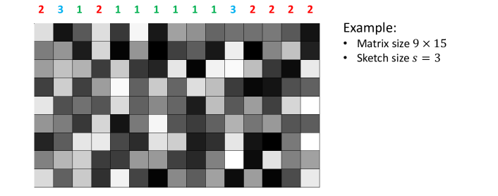
(a) Hash each column with a value uniformly sampled from $[s]=\{1,2,3\}$.

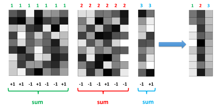
(b) Flip the sign of each column with probability $50\%$, and then sum up columns with the same hash value.

Figure 3.1: Count sketch in the map-reduce fashion.

3.2.3 Count Sketch

Count sketch stems from the data stream literature [4; 26]. It was applied to speedup matrix computation by [6; 21]. We describe in the following the count sketch for matrix data.

There are different ways to implementing count sketch. This paper describe two quite different ways and refer to them as “map-reduce fashion” and “streaming fashion”. Of course, the two are equivalent.

• The map-reduce fashion has three steps. First, hash each column with a discrete value uniformly sampled from $[s]$. Second, flip the sign of each column with probability $50\%$. Third, sum up columns with the same hash value. This procedure is illustrated in Figure 3.1. As its name suggests, this approach naturally fits the map-reduce systems.

• The streaming fashion has two steps. First, initialize ${\bf C}$ to be the $m\times s$ all-zero matrix. Second, for each column of ${\bf A}$, flip its sign with probability $50\%$, and add it to a uniformly selected column of ${\bf C}$. It is described in Algorithm 1 an illustrated in Figure 3.2. It can be implemented in 9 lines of MATLAB code as below. The streaming fashion implementation keeps the sketch ${\bf C}$ in memory and scans the data ${\bf A}$ in only one pass. If ${\bf A}$ does not fit in memory, this approach is better than the map-reduce fashion for it scans the columns sequentially. If ${\bf A}$ is sparse matrix, randomly accessing the entries may not be efficient, and thus it is better to accessing the column sequentially.

⬇

1function [C] = CountSketch(A, s) % the streaming fashion

2[m, n] = size(A);

3sgn = randi(2, [1, n]) * 2 - 3; % one half are +1 and the rest are -1

4A = bsxfun(@times, A, sgn); % flip the signs of each column w.p. 50%

5ll = randsample(s, n, true); % sample n items from [s] with replacement

6C = zeros(m, s); % initialize C

7for j = 1: n

8 C(:, ll(j)) = C(:, ll(j)) + A(:, j);

9end

Algorithm 1 Count Sketch in the Streaming Fashion.

1:  input: ${\bf A}\in{\mathbb{R}}^{m\times n}$.

2:  Initialize ${\bf C}$ to be an $m\times s$ all-zero matrix;

3:  for $i=1$ to $n$ do

4:        sample $l$ from the set $[s]$ uniformly at random;

5:        sample $g$ from the set $\{+1,-1\}$ uniformly at random;

6:        update the $l$-th column of ${\bf C}$ by ${\bf c}_{:l}\longleftarrow{\bf c}_{:l}+g{\bf a}_{:i}$;

7:  end for

8:  return  ${\bf C}\in{\mathbb{R}}^{m\times s}$.

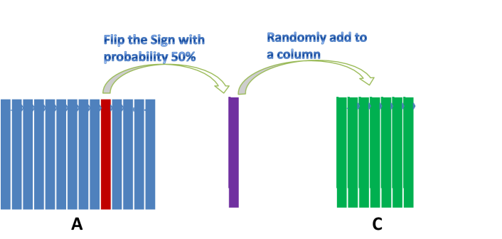
Figure 3.2: Count sketch in the streaming fashion.

The readers may have noticed that count sketch does not explicitly form the sketching matrix ${\bf S}$. In fact, ${\bf S}$ is such a matrix that each row has only one nonzero entry. In the example of Figure 3.1, the matrix ${\bf S}^{T}$ can be explicitly expressed as

$${\bf S}^{T}\;=\;\left[\begin{array}[]{ccccccccccccccc}0&0&1&0&1&-1&1&-1&-1&1&0&0&0&0&0\\ -1&0&0&-1&0&0&0&0&0&0&0&-1&1&-1&-1\\ 0&-1&0&0&0&0&0&0&0&0&1&0&0&0&0\\ \end{array}\right].$$

Count sketch has the following properties:

• Time cost: ${\mathcal{O}}(\mathrm{nnz}({\bf A}))$

• Memory cost: ${\mathcal{O}}(ms)$. When ${\bf A}$ does not fit in memory, the algorithm keeps only ${\bf C}$ in memory and goes one pass through the columns of ${\bf A}$.

• Theoretical guarantees

  1. When $s={\mathcal{O}}({m^{2}}/{\epsilon^{2}})$, the subspace embedding property holds with $\gamma=1+\epsilon$ with high probability.

  2. When $s={\mathcal{O}}({k}/{\epsilon}+k^{2})$, the low-rank approximation property holds with $\eta=1+\epsilon$ relative error with high probability.

• Advantage: the count sketch is very efficient, especially when ${\bf A}$ is sparse.

• Disadvantage: compared with Gaussian projection, the count sketch requires larger $s$ to attain the same accuracy. One simple improvement is to combine the count sketch with Gaussian projection or SRHT.

3.2.4 GaussianProjection + CountSketch

Let ${\bf S}_{sc}$ be $n\times s_{cs}$ count sketch matrix, ${\bf S}_{gp}$ be $s_{cs}\times s$ Gaussian projection matrix, and ${\bf S}={\bf S}_{cs}{\bf S}_{gp}\in{\mathbb{R}}^{n\times s}$. Then ${\bf S}$ satisfies the following properties.

• Time complexity: the matrix product ${\bf A}{\bf S}$ can be computed in

  $${\mathcal{O}}\big{(}\underbrace{\mathrm{nnz}({\bf A})}_{\textrm{count sketch}}+\underbrace{ms_{cs}s}_{\textrm{Gaussian projection}}\big{)}$$

  time.

• Theoretical properties:

  1. When $s_{cs}={\mathcal{O}}(m^{2}/\epsilon^{2})$ and $s={\mathcal{O}}(m/\epsilon^{2})$, the GaussianProjection+CountSketch matrix ${\bf S}$ satisfy the subspace embedding property with $\gamma=1+\epsilon$ holds with high probability.

  2. When $s_{cs}={\mathcal{O}}(k^{2}+k/\epsilon)$ and $s={\mathcal{O}}(k/\epsilon)$, the GaussianProjection+CountSketch matrix ${\bf S}$ satisfies the low-rank approximation property with $\eta=1+\epsilon$ [2, Lemma 12].

• Advantages:

  1. the size of GaussianProjection+CountSketch is as small as Gaussian projection.

  2. the time complexity is much lower than Gaussian projection when $n\gg m$.

3.3 Column Selection

This section presents three column selection techniques: uniform sampling, leverage score sampling, and local landmark selection. Different from random projection, column selection do not have to visit every entry of ${\bf A}$, and column selection preserves the sparsity/non-negativity properties of ${\bf A}$.

3.3.1 Uniform Sampling

Uniform sampling is the most efficient way to form a sketch. The most important advantage is that uniform sampling forms a sketch without seeing the whole data matrix. When applied to kernel methods, uniform sampling avoids computing every entry of the kernel matrix.

The performance of uniform sampling is data-dependent. When the leverage scores (defined in Section 3.3.2) are uniform, or equivalently, the matrix coherence (namely the greatest leverage score) is small, uniform sampling has good performance. The analysis of uniform sampling can be found in [12; 13].

3.3.2 Leverage Score Sampling

Before studying leverage score sampling, let’s first define leverage scores. Let ${\bf A}$ be an $m\times n$ matrix, with $\rho=\mathrm{rank}({\bf A})<n$, and ${\bf V}\in{\mathbb{R}}^{n\times\rho}$ be the right singular vectors. The (column) leverage scores of ${\bf A}$ are defined by

$$l_{i}\;:=\;\|{\bf v}_{i:}\|_{2}^{2},\qquad\textrm{ for }i=1,\cdots,n.$$

Leverage score sampling is to select each columns of ${\bf A}$ with probability proportional to its leverage scores. (Sometimes each selected column should be scaled by $\sqrt{\frac{\rho}{sl_{i}}}$.) It can be roughly implemented in 8 lines MATLAB code.

⬇

1function [C, idx] = LeverageScoreSampling(A, s)

2n = size(A, 2);

3[~, ~, V] = svd(A, ’econ’);

4leveragescores = sum(V.^2, 2);

5prob = leveragescores / sum(leveragescores);

6idx = randsample(n, s, true, prob);

7idx = unique(idx); % eliminate duplicates

8C = A(:, idx);

There are a few things to remark:

• To sample columns according to the leverage scores of ${\bf A}_{k}$ where $k\ll m,n$, Line 3 can be replaced by

  ⬇

  3[~, ~, V] = svds(A, k);

• Theoretical properties

  1. When $s={\mathcal{O}}(m/\epsilon+m\log m)$, the leverage score sampling satisfies the subspace embedding property with $\gamma=1+\epsilon$ holds with high probability.

  2. When $s={\mathcal{O}}(k/\epsilon+k\log k)$, the leverage score sampling (according to the leverage scores of ${\bf A}_{k}$) satisfies the low-rank approximation property with $\eta=1+\epsilon$.

• Computing the leverage scores is as expensive as computing SVD, so leverage score sampling is not a practical way to sketch the matrix ${\bf A}$ itself.

• When the leverage scores are near uniform, there is little difference between uniform sampling and leverage score sampling.

3.3.3 Local Landmark Selection

Local landmark selection is a very effective heuristic for finding representative columns. Zhang and Kwok [36] proposed to set $k=s$ and run $k$-means or $k$-centroids clustering algorithm to cluster the columns of ${\bf A}$ to $s$ class, and use the $s$ centroids as the sketch of ${\bf A}$. This heuristic works very well in practice, though it has little theoretical guarantee.

There are several tricks to make the local landmark selection more efficient.

• One can simply solve $k$-centroids clustering approximately rather than accurately. For example, it is unnecessary to wait for $k$-centroids clustering to converge; running $k$-centroids for a few iterations suffices.

• When $n$ is large, one can uniformly sample a subset of the data, e.g. $\max\{0.2n,20s\}$ data points, and perform local landmark selection on this smaller dataset.

• In supervised learning problems, each datum ${\bf a}_{i}$ is associated with a label $y_{i}$. We can partition the data to $g$ groups according to the labels and run $k$-centroids clustering independently on the data in each group. In this way, $s=gk$ data points are selected as a sketch of ${\bf A}$.

Chapter 4 Regression

Let ${\bf A}$ be an $n\times d$ ($n\geq d$) matrix whose rows correspond to data and columns correspond to features, and let ${\bf b}\in{\mathbb{R}}^{n}$ contain the response/label of each datum. The least squares regression (LSR)

$$\min_{\bf x}\;\|{\bf A}{\bf x}-{\bf b}\|_{2}^{2}$$ (4.1)

is a ubiquitous problem in statistics, computer science, economics, etc. When $n\gg d$, LSR can be efficiently solved using randomized algorithms.

4.1 Standard Solutions

The least squares regression (LSR) problem (4.1) has closed form solution

$${\bf x}^{\star}\;=\;{\bf A}^{\dagger}{\bf b}.$$

The Moore-Penrose inverse can be computed by SVD which costs ${\mathcal{O}}(nd^{2})$ time.

LSR can also be solved by numerical algorithms such as the conjugate gradient (CG) algorithm, and machine-precision can be attained in a reasonable number of iterations. Let $\kappa({\bf A}):=\frac{\sigma_{1}({\bf A})}{\sigma_{d}({\bf A})}$ be the condition number of ${\bf A}$. The convergence of CG depends on $\kappa({\bf A})$:

$$\frac{\|{\bf A}({\bf x}^{(t)}-{\bf x}^{\star})\|_{2}^{2}}{\|{\bf A}({\bf x}^{(0)}-{\bf x}^{\star})\|_{2}^{2}}\;\leq\;2\bigg{(}\frac{\kappa({\bf A})-1}{\kappa({\bf A})+1}\bigg{)}^{t},$$

where ${\bf x}^{(t)}$ is the model in the $t$-th iteration of CG. The per-iteration time cost of CG is ${\mathcal{O}}(\mathrm{nnz}({\bf A}))$. To attain $\|{\bf A}({\bf x}^{(t)}-{\bf x}^{\star})\|_{2}^{2}\leq\epsilon$, the number of iteration is roughly

$$\Big{(}\log\frac{1}{\epsilon}+\log(\textrm{InitialError})\Big{)}\frac{\kappa({\bf A})-1}{2}.$$

Since the time cost of CG heavily depends on the unknown condition number $\kappa({\bf A})$, CG can be very slow if ${\bf A}$ is ill-conditioned.

4.2 Inexact Solution

Any sketching matrix ${\bf S}\in{\mathbb{R}}^{n\times s}$ can be used to solve LSR approximately as long as it satisfies the subspace embedding property. We consider the following LSR problem:

$$\tilde{\bf x}\;=\;\min_{\bf x}\;\|\underbrace{({\bf S}^{T}{\bf A})}_{s\times d}{\bf x}-{\bf S}^{T}{\bf b}\|_{2}^{2},$$ (4.2)

which can be solved in ${\mathcal{O}}(sd^{2})$ time.

If ${\bf S}$ is a Gaussian projection matrix, SRHT matrix, count sketch, or leverage score sampling matrix, and $s=\mathrm{poly}(d/\epsilon)$ for any error parameter $\epsilon\in(0,1]$, then

$$\|{\bf A}\tilde{\bf x}-{\bf b}\|_{2}^{2}\;\leq\;(1+\epsilon)^{2}\min_{\bf x}\|{\bf A}{\bf x}-{\bf b}\|_{2}^{2}$$

is guaranteed.

4.2.1 Implementation

If ${\bf S}$ is count sketch matrix, the inexact LSR algorithm can be implemented in 5 lines of MATLAB code. Here CountSketch is a MATLAB function described in Section 3.2.3. The total time cost is ${\mathcal{O}}(\mathrm{nnz}({\bf A})+\mathrm{poly}(d/\epsilon))$ and memory cost is ${\mathcal{O}}(\mathrm{poly}(d/\epsilon))$, which are lower than the cost of exact LSR when $d\ll n$.

⬇

1function [xtilde] = InexactLSR(A, b, s)

2d = size(A, 2);

3sketch = (CountSketch([A, b]’, s))’;

4Asketch = sketch(:, 1:d); % Asketch = S’ * A

5bsketch = sketch(:, end); % bsketch = S’ * b

6xtilde = Asketch \ bsketch;

There are a few things to remark:

• The inexact LSR is useful only when $n=\Omega(d/\epsilon+d^{2})$.

• The size of sketch $s$ is a polynomial function of $\epsilon^{-1}$ rather than logarithm of $\epsilon^{-1}$, thus the algorithm cannot attain high precision.

4.2.2 Theoretical Explanation

By the subspace embedding property, it can be easily shown that $\tilde{\bf x}$ is a good solution. Let ${\bf D}=[{\bf A},{\bf b}]\in{\mathbb{R}}^{n\times(d+1)}$ and ${\bf z}=[{\bf x};-1]\in{\mathbb{R}}^{n+1}$. Then

$${\bf A}{\bf x}-{\bf b}={\bf D}{\bf z}\qquad\textrm{ and }\qquad{\bf S}^{T}{\bf A}{\bf x}-{\bf S}^{T}{\bf b}={\bf S}^{T}{\bf D}{\bf z},$$

and the subspace embedding property indicates $\frac{1}{\eta}\|{\bf D}{\bf z}\|_{2}^{2}\leq\|{\bf S}^{T}{\bf D}{\bf z}\|_{2}^{2}\leq\eta\|{\bf D}{\bf z}\|_{2}^{2}$ for all ${\bf z}$. Thus

$$\frac{1}{\eta}\|{\bf A}\tilde{\bf x}-{\bf b}\|_{2}^{2}\;\leq\;\|{\bf S}^{T}({\bf A}\tilde{\bf x}-{\bf b})\|_{2}^{2}\qquad\textrm{ and }\qquad\|{\bf S}^{T}({\bf A}{\bf x}^{\star}-{\bf b})\|_{2}^{2}\;\leq\;\eta\|{\bf A}{\bf x}^{\star}-{\bf b}\|_{2}^{2}$$

The optimality of $\tilde{\bf x}$ indicates $\|{\bf S}^{T}({\bf A}\tilde{\bf x}-{\bf b})\|_{2}^{2}\leq\|{\bf S}^{T}({\bf A}{\bf x}^{\star}-{\bf b})\|_{2}^{2}$, and thus

$$\frac{1}{\eta}\|{\bf A}\tilde{\bf x}-{\bf b}\|_{2}^{2}\;\leq\;\|{\bf S}^{T}({\bf A}\tilde{\bf x}-{\bf b})\|_{2}^{2}\;\leq\;\|{\bf S}^{T}({\bf A}{\bf x}^{\star}-{\bf b})\|_{2}^{2}\;\leq\;\eta\|{\bf A}{\bf x}^{\star}-{\bf b}\|_{2}^{2}.$$

$$\Rightarrow\|{\bf A}\tilde{\bf x}-{\bf b}\|_{2}^{2}\;\leq\;\eta^{2}\|{\bf A}{\bf x}^{\star}-{\bf b}\|_{2}^{2}.$$

Therefore, as long as ${\bf S}$ satisfies the subspace embedding property, the approximate solution to LSR is nearly as good as the optimal solution (in terms of objective function value).

4.3 Machine-Precision Solution

Randomized algorithms can also be applied to find machine-precision solution to LSR, and the time complexity is lower than the standard solutions. The state-of-the-art algorithm [18] is based on very similar idea described in this section.

4.3.1 Basic Idea: Preconditioning

We have discussed previously that the time cost of the conjugate gradient (CG) algorithm is roughly

$$\frac{{\color[rgb]{1,0,0}\kappa({\bf A})}-1}{2}\Big{(}\log\frac{1}{\epsilon}+\log(\textrm{InitialError})\Big{)}\mathrm{nnz}({\bf A}),$$

which dependents on the condition number of ${\bf A}$. To make CG efficient, one can find a $d\times d$ preconditioning matrix ${\bf T}$ such that $\kappa({\bf A}{\bf T})$ is small, solve

$${\bf z}^{\star}\;=\;\mathop{\rm argmin}_{\bf z}\|({\bf A}{\bf T}){\bf z}-{\bf b}\|_{2}^{2}$$ (4.3)

by CG, and let ${\bf x}^{\star}={\bf T}{\bf z}^{\star}$. In this way, the time cost of CG is roughly

$$\frac{{\color[rgb]{1,0,0}\kappa({\bf A}{\bf T})}-1}{2}\Big{(}\log\frac{1}{\epsilon}+\log(\textrm{InitialError})\Big{)}\mathrm{nnz}({\bf A}).$$

If $\kappa({\bf A}{\bf T})$ is a small constant, e.g. $\kappa({\bf A}{\bf T})=2$, then (4.3) can be very efficiently solved by CG.

Now let’s consider how to find the preconditioning matrix ${\bf T}$. Let ${\bf A}={\bf Q}_{\bf A}{\bf R}_{\bf A}$ be the QR decomposition. Obviously ${\bf T}={\bf R}_{\bf A}^{-1}$ is a perfect preconditioning matrix because $\kappa({\bf A}{\bf R}_{\bf A}^{-1})=\kappa({\bf Q}_{\bf A})=1$. Unfortunately, the preconditioning matrix ${\bf T}={\bf R}_{\bf A}^{-1}$ is not a practical choice because computing the QR decomposition is as expensive as solving LSR.

Woodruff [34] proposed to use sketching to find ${\bf R}_{\bf A}$ approximately in ${\mathcal{O}}(\mathrm{nnz}({\bf A})+\mathrm{poly}(d))$ time. Let ${\bf S}\in{\mathbb{R}}^{n\times s}$ be a sketching matrix and form ${\bf Y}={\bf S}^{T}{\bf A}$. Let ${\bf Y}={\bf Q}_{\bf Y}{\bf R}_{\bf Y}$ be the QR decomposition of ${\bf Y}$. Theory shows that the sketch size $s={\mathcal{O}}(d^{2})$ suffices for $\kappa({\bf A}{\bf R}_{\bf Y}^{-1})\leq 2$ holding with high probability. Thus ${\bf R}_{\bf Y}^{-1}\in{\mathbb{R}}^{d\times d}$ is a good preconditioning matrix.

Algorithm 1 Machine-Precision Solution to LSR.

1:  input: ${\bf A}\in{\mathbb{R}}^{n\times d}$, ${\bf b}\in{\mathbb{R}}^{n}$, and step size $\theta$.

2:  Draw a sketching matrix ${\bf S}\in{\mathbb{R}}^{n\times s}$ where $s={\mathcal{O}}(d^{2})$;

3:  Form the sketch ${\bf Y}={\bf S}^{T}{\bf A}\in{\mathbb{R}}^{s\times d}$;

4:  Compute the QR decomposition ${\bf Y}={\bf Q}_{\bf Y}{\bf R}_{\bf Y}$;

5:  Compute the preconditioning matrix ${\bf T}={\bf R}_{\bf Y}^{-1}$;

6:  Compute the initial solution ${\bf z}^{(0)}=({\bf S}^{T}{\bf A}{\bf T})^{\dagger}({\bf S}^{T}{\bf b})={\bf Q}_{\bf Y}^{T}({\bf S}^{T}{\bf b})$;

7:  for $t=1,\cdots,{\mathcal{O}}(\log\epsilon^{-1})$ do

8:        ${\bf r}^{(t)}={\bf b}-{\bf A}{\bf T}{\bf z}^{(t-1)}$ ;      // the residual

9:        ${\bf z}^{(t)}={\bf z}^{(t-1)}+\theta{\bf T}^{T}{\bf A}^{T}{\bf r}^{(t)}$;   // gradient descent

10:  end for

11:  return  ${\bf x}^{\star}={\bf T}{\bf z}^{(t)}\in{\mathbb{R}}^{d}$.

4.3.2 Algorithm Description

The algorithm is described in Algorithm 1. We first form a sketch ${\bf Y}={\bf S}^{T}{\bf A}\in{\mathbb{R}}^{s\times d}$ and compute its QR decomposition ${\bf Y}={\bf Q}_{\bf Y}{\bf R}_{\bf Y}$. We can use this QR decomposition to find the initial solution ${\bf z}^{(0)}$ and the preconditioning matrix ${\bf T}={\bf R}_{\bf Y}^{-1}$. If we set $s={\mathcal{O}}(d^{2})$, the initial solution is only constant times worse than the optimal in terms of objective function value. Theory also ensures that the condition number $\kappa({\bf A}{\bf T})\leq 2$. With the good initialization and good condition number, the vanilla gradient descent or CG takes only ${\mathcal{O}}(\log\epsilon^{-1})$ steps to attain $1+\epsilon$ solution. Notice that Lines 8 and 9 in the algorithm should be cautiously implemented. Do not compute the matrix product ${\bf A}{\bf T}$ because it would take ${\mathcal{O}}(\mathrm{nnz}({\bf A})d)$ time!

4.4 Extension: CX-Type Regression

Given any matrix ${\bf A}\in{\mathbb{R}}^{m\times n}$, CX decomposition considers decomposing ${\bf A}$ into ${\bf A}\approx{\bf C}{\bf X}^{\star}$, where ${\bf C}\in{\mathbb{R}}^{m\times c}$ is a sketch of ${\bf A}$ and ${\bf X}^{\star}\in{\mathbb{R}}^{c\times n}$ is computed by

$${\bf X}^{\star}\;=\;\mathop{\rm argmin}_{\bf X}\,\big{\|}{\bf A}-{\bf C}{\bf X}\big{\|}_{F}^{2}\;=\;{\bf C}^{\dagger}{\bf A}.$$

It takes ${\mathcal{O}}(mnc)$ time to compute ${\bf X}^{\star}$. If $c\ll m$, this problem can be solved more efficiently by sketching. Specifically, we can draw a sketching matrix ${\bf S}\in{\mathbb{R}}^{m\times s}$ and compute the approximate solution

$$\tilde{\bf X}\;=\;\mathop{\rm argmin}_{\bf X}\|\underbrace{{\bf S}^{T}{\bf C}}_{s\times c}\underbrace{{\bf X}}_{c\times n}-\underbrace{{\bf S}^{T}{\bf A}}_{s\times n}\|_{F}^{2}\;=\;({\bf S}^{T}{\bf C})^{\dagger}({\bf S}^{T}{\bf A})$$

If ${\bf S}$ is a count sketch matrix, we set $s={\mathcal{O}}(c/\epsilon+c^{2})$; if ${\bf S}$ samples columns according to the row leverage scores of ${\bf C}$, we set $s={\mathcal{O}}(c/\epsilon+c\log c)$. It holds with high probability that

$$\big{\|}{\bf A}-{\bf C}\tilde{\bf X}\big{\|}_{F}^{2}\;\leq\;(1+\epsilon)\,\min_{\bf X}\big{\|}{\bf A}-{\bf C}{\bf X}\big{\|}_{F}^{2}.$$

4.5 Extension: CUR-Type Regression

A more complicated problem has also been considered in the literature [25; 29; 24]:

$${\bf X}^{\star}\;=\;\mathop{\rm argmin}_{\bf X}\|\underbrace{{\bf C}}_{n\times c}\underbrace{{\bf X}}_{c\times r}\underbrace{{\bf R}}_{r\times n}-\underbrace{{\bf A}}_{m\times n}\|_{F}^{2}$$ (4.4)

where $c,r\ll m,n$. The solution is:

$${\bf X}^{\star}\;=\;{\bf C}^{\dagger}{\bf A}{\bf R}^{\dagger},$$

which cost ${\mathcal{O}}(mn\cdot\min\{c,r\})$ time. Wang et al. [31] proposed an algorithm to solve (4.4) approximately by

$$\tilde{\bf X}\;=\;\mathop{\rm argmin}_{\bf X}\|{\bf S}_{C}^{T}({\bf C}{\bf X}{\bf R}-{\bf A}){\bf S}_{R}\|_{F}^{2}$$

where ${\bf S}_{C}\in{\mathbb{R}}^{m\times s_{c}}$ and ${\bf S}_{R}\in{\mathbb{R}}^{n\times s_{r}}$ are leverage score sampling matrices. When $s_{c}=c\sqrt{q/\epsilon}$ and $s_{r}=r\sqrt{q/\epsilon}$ (where $q=\min\{m,n\}$), it holds with high probability that

$$\|{\bf C}\tilde{\bf X}{\bf R}-{\bf A}\|_{F}^{2}\;\leq\;(1+\epsilon)\,\min_{\bf X}\|{\bf C}{\bf X}{\bf R}-{\bf A}\|_{F}^{2}.$$

The total time cost is

$${\mathcal{O}}(s_{c}s_{r}\cdot\min\{c,r\})\;=\;{\mathcal{O}}(cr\epsilon^{-1}\cdot\min\{m,n\}\cdot\min\{c,r\})$$

time, which is useful when $\max\{m,n\}\gg c,r$. The algorithm can be implemented in 4 lines of MATLAB code:

⬇

1function [Xtilde] = InexactCurTypeRegression(C, R, A, sc, sr)

2[~, idxC] = LeverageScoreSampling(C’, sc);

3[~, idxR] = LeverageScoreSampling(R, sr);

4Xtilde = pinv(C(idxC, :)) * A(idxC, idxR) * pinv(R(:, idxR));

Here the function “$\mathrm{LeverageScoreSampling}$” is described in Section 3.3.2. Empirically, setting $s_{1}=s_{2}={\mathcal{O}}(d_{1}+d_{2})$ suffices for high precision. The experiments in [31] indicates that uniform sampling performs equally well as leverage score sampling.

Chapter 5 Rank $k$ Singular Value Decomposition

This chapter considers the $k$-SVD of a large scale matrix ${\bf A}\in{\mathbb{R}}^{m\times n}$, which may not fit in memory.

5.1 Standard Solutions

The standard solutions to $k$-SVD include the power iteration algorithm and the Krylov subspace methods. Their time complexities are considered to be $\tilde{\mathcal{O}}(mnk)$, where the $\tilde{\mathcal{O}}$ notation hides parameters such as the spectral gap and logarithm of error tolerance. Here we introduce a simplified version of the block Lanczos method [19] which costs time ${\mathcal{O}}(mnkq)$, where $q=\log\frac{n}{\epsilon}$ is the number of iterations, and the inherent constant depends weakly on the spectral gap. The block Lanczos algorithm is described in Algorithm 1 can be implemented in 18 lines of MATLAB code.

⬇

1function [U, S, V] = BlockLanczos(A, k, q)

2s = 2 * k; % can be tuned

3[m, n] = size(A);

4C = A * randn(n, s);

5Krylov = zeros(m, s * q);

6Krylov(:, 1:s) = C;

7for i = 2: q

8 C = A’ * C;

9 C = A * C;

10 [C, ~] = qr(C, 0); % optional

11 Krylov(:, (i-1)*s+1: i*s) = C;

12end

13[Q, ~] = qr(Krylov, 0);

14[Ubar, S, V] = svd(Q’ * A, ’econ’);

15Ubar = Ubar(:, 1:k);

16S = S(1:k, 1:k);

17V = V(:, 1:k);

18U = Q * Ubar;

Although the block Lanczos algorithm can attain machine precision, it inevitably goes many passes through ${\bf A}$, and it is thus slow when ${\bf A}$ does not fit in memory.

Facing large-scale data, we must trade off between precision and computational costs. We are particularly interested in approximate algorithm that satisfies:

1. The algorithm goes constant passes through ${\bf A}$. Then ${\bf A}$ can be stored in large volume disks, and there are only constant swaps between disk and memory.

2. The algorithm only keeps a small-scale sketch of ${\bf A}$ in memory.

3. The time cost is ${\mathcal{O}}(mnk)$ or lower.

Algorithm 1 $k$-SVD by the Block Lanczos Algorithm.

1:  Input: an $m\times n$ matrix ${\bf A}$ and the target rank $k$.

2:  Set $s=k+{\mathcal{O}}(1)$ be the over-sampling parameter;

3:  Set $q={\mathcal{O}}(\log\frac{n}{\epsilon})$ be the number of iteration;

4:  Draw a $n\times s$ sketching matrix ${\bf S}$;

5:  ${\bf C}={\bf A}{\bf S}$;

6:  Set ${\bf K}=\big{[}{\bf C},\;({\bf A}{\bf A}^{T}){\bf C},\;({\bf A}{\bf A}^{T})^{2}{\bf C},\;\cdots,\;({\bf A}{\bf A}^{T})^{q-1}{\bf C}\big{]}$;

7:  QR decomposition: $[\underbrace{{\bf Q}_{\bf C}}_{m\times sq},{\bf R}_{\bf C}]=qr(\underbrace{{\bf K}}_{m\times sq})$;

8:  SVD: $[\underbrace{\bar{\bf U}}_{sq\times sq},\underbrace{\mbox{\boldmath$\Sigma$\unboldmath}}_{sq\times sq},\underbrace{{\bf V}}_{n\times sq}]=svd(\underbrace{{\bf Q}_{\bf C}^{T}{\bf A}}_{s\times n})$;

9:  Retain the top $k$ components of $\bar{\bf U}$, $\Sigma$, and ${\bf V}$ to form $sq\times k$, $k\times k$, $n\times k$ matrices;

10:  ${\bf U}={\bf Q}\bar{\bf U}\in{\mathbb{R}}^{m\times k}$;

11:  return  ${\bf U}\mbox{\boldmath$\Sigma$\unboldmath}{\bf V}^{T}\approx{\bf A}_{k}$.

5.2 Prototype Randomized $k$-SVD Algorithm

This section describes a randomized algorithm that computes the $k$-SVD of ${\bf A}$ up to $1+\epsilon$ Frobenius norm relative error. The algorithm is proposed by [14], and it is described in Algorithm 2.

Algorithm 2 Prototype Randomized $k$-SVD Algorithm.

1:  Input: an $m\times n$ matrix ${\bf A}$ and the target rank $k$.

2:  Draw a $n\times s$ sketching matrix ${\bf S}$ where $s={\mathcal{O}}(\frac{k}{\epsilon})$;

3:  ${\bf C}={\bf A}{\bf S}$;

4:  QR decomposition: $[\underbrace{{\bf Q}_{\bf C}}_{m\times s},{\bf R}_{\bf C}]=qr(\underbrace{{\bf C}}_{m\times s})$;

5:  $k$-SVD: $[\underbrace{\bar{\bf U}}_{s\times k},\underbrace{\tilde{}\mbox{\boldmath$\Sigma$\unboldmath}}_{k\times k},\underbrace{\tilde{\bf V}}_{n\times k}]=svds(\underbrace{{\bf Q}_{\bf C}^{T}{\bf A}}_{s\times n},k)$;

6:  $\tilde{\bf U}={\bf Q}_{\bf C}\bar{\bf U}\in{\mathbb{R}}^{m\times k}$;

7:  return  $\tilde{\bf U}\tilde{}\mbox{\boldmath$\Sigma$\unboldmath}\tilde{\bf V}^{T}\approx{\bf A}_{k}$.

5.2.1 Theoretical Explanation

If ${\bf C}={\bf A}{\bf S}\in{\mathbb{R}}^{m\times s}$ is a good sketch of ${\bf A}$, the column space of ${\bf C}$ should roughly contain the columns of ${\bf A}_{k}$—this is the low-rank approximation property. If ${\bf S}\in{\mathbb{R}}^{n\times s}$ is Gaussian projection matrix or count sketch and $s={\mathcal{O}}(k/\epsilon)$, then the low-rank approximation property

$$\min_{\mathrm{rank}({\bf Z})\leq k}\|{\bf C}{\bf Z}-{\bf A}\|_{F}^{2}\;\leq\;(1+\epsilon)\|{\bf A}-{\bf A}_{k}\|_{F}^{2}$$ (5.1)

holds in expectation.

5.2.2 Algorithm Derivation

Let ${\bf Q}_{\bf C}$ be any orthonormal bases of ${\bf C}$. Since the column space of ${\bf C}$ is the same to the column space of ${\bf Q}_{\bf C}$, the minimization problem in (5.1) can be equivalently converted to

$${\bf X}^{\star}\;=\;\mathop{\rm argmin}_{\mathrm{rank}({\bf X})\leq k}\|\underbrace{{\bf Q}_{\bf C}}_{m\times s}\underbrace{{\bf X}}_{s\times n}-\underbrace{{\bf A}}_{m\times n}\|_{F}^{2}\;=\;({\bf Q}_{\bf C}^{T}{\bf A})_{k}.$$ (5.2)

Here the second equality is a well known fact. The matrix ${\bf A}_{k}$ is well approximated by $\tilde{\bf A}_{k}:={\bf Q}_{\bf C}{\bf X}^{\star}$, so we need only to find the $k$-SVD of $\tilde{\bf A}_{k}$:

$$\tilde{\bf A}_{k}\;:=\;\underbrace{{\bf Q}_{\bf C}}_{m\times s}\underbrace{{\bf X}^{\star}}_{s\times n}\;=\;{\bf Q}_{\bf C}\underbrace{({\bf Q}_{\bf C}^{T}{\bf A})_{k}}_{:=\bar{\bf U}{\tilde{\bf\Sigma}}\tilde{\bf V}^{T}}\;=\;\underbrace{{\bf Q}_{\bf C}\bar{\bf U}}_{:=\tilde{\bf U}}\tilde{}\mbox{\boldmath$\Sigma$\unboldmath}\tilde{\bf V}^{T}\;=\;\underbrace{\tilde{\bf U}}_{m\times k}\underbrace{\tilde{}\mbox{\boldmath$\Sigma$\unboldmath}}_{k\times k}\underbrace{\tilde{\bf V}^{T}}_{k\times n}.$$

It is easy to check that $\tilde{\bf U}$ and $\tilde{\bf V}$ have orthonormal columns and $\tilde{}\mbox{\boldmath$\Sigma$\unboldmath}$ is a diagonal matrix. Notice that the accuracy of the randomized $k$-SVD depends only on the quality of the sketch matrix ${\bf C}$.

5.2.3 Implementation

The algorithm is described in Algorithm 2 and can be implemented in 5 lines of MATLAB code. Here $s={\mathcal{O}}(\frac{k}{\epsilon})$ is the size of the sketch.

⬇

1function [Utilde, Stilde, Vtilde] = ksvdPrototype(A, k, s)

2C = CountSketch(A, s);

3[Q, R] = qr(C, 0);

4[Ubar, Stilde, Vtilde] = svds(Q’ * A, k);

5Utilde = Q * Ubar;

Empirically, using “$\mathrm{svd(Q^{\prime}*A,\,^{\prime}econ^{\prime})}$” followed by discarding the $k+1$ to $s$ components should be faster than the “$\mathrm{svds}$” function in Line 4.

The algorithm has the following properties:

1. The algorithm goes 2 passes through ${\bf A}$;

2. The algorithm only keeps an $m\times{\mathcal{O}}(\frac{k}{\epsilon})$ sketch ${\bf C}$ in memory;

3. The time cost is ${\mathcal{O}}(\mathrm{nnz}({\bf A})k/\epsilon)$.

5.3 Faster Randomized $k$-SVD

The prototype algorithm spends most of its time on solving (5.2); if (5.2) can be solved more efficiently, the randomized $k$-SVD can be even faster. The readers may have noticed that (5.2) is the least squares regression (LSR) problem discussed in Section 4.4. Yes, we can solve (5.2) efficiently by the inexact LSR algorithm presented in the previous section.

5.3.1 Theoretical Explanation

Now we draw a $m\times p$ GaussianProjection+CountSketch matrix ${\bf P}$ and solve this problem:

$$\tilde{\bf X}\;=\;\mathop{\rm argmin}_{\mathrm{rank}({\bf X})\leq k}\|\underbrace{{\bf P}^{T}{\bf Q}_{\bf C}}_{p\times s}\underbrace{{\bf X}}_{s\times n}-\underbrace{{\bf P}^{T}{\bf A}}_{p\times n}\|_{F}^{2}.$$ (5.3)

To understand this trick, the readers can retrospect the extension of LSR in Section 4.4. Let

$${\bf P}=\underbrace{{\bf P}_{cs}}_{m\times p_{cs}}\underbrace{{\bf P}_{srht}}_{p_{cs}\times p}$$

where $p_{cs}={\mathcal{O}}(k/\epsilon+k^{2})$ and $p={\mathcal{O}}(k/\epsilon)$. The subspace embedding property of RSHT+CountSketch [6, Theorem 46] implies that

$$(1+\epsilon)^{-1}\|{\bf Q}_{\bf C}\tilde{\bf X}-{\bf A}\|_{F}^{2}\;\leq\;\|{\bf P}^{T}({\bf Q}_{\bf C}\tilde{\bf X}-{\bf A})\|_{F}^{2}\;\leq\;\|{\bf P}^{T}({\bf Q}_{\bf C}{\bf X}^{\star}-{\bf A})\|_{F}^{2}\;\leq\;(1+\epsilon)\|{\bf Q}_{\bf C}{\bf X}^{\star}-{\bf A}\|_{F}^{2},$$

$$\Rightarrow\;\|{\bf Q}_{\bf C}\tilde{\bf X}-{\bf A}\|_{F}^{2}\;\leq\;(1+\epsilon)^{2}\|{\bf Q}_{\bf C}{\bf X}^{\star}-{\bf A}\|_{F}^{2}\;\leq\;(1+\epsilon)^{3}\|{\bf A}-{\bf A}_{k}\|_{F}^{2}.$$

Here the second inequality follows from the optimality of $\tilde{\bf X}$, and the last inequality follows from the low-rank approximation property of the sketch ${\bf C}={\bf A}{\bf S}$. Thus, by solving (5.3) we get $k$-SVD up to $1+{\mathcal{O}}(\epsilon)$ Frobenius norm relative error.

5.3.2 Algorithm Derivation

The faster randomized $k$-SVD is described in Algorithm 3 and derived in the following. The algorithm solves

$$\tilde{\bf X}\;=\;\mathop{\rm argmin}_{\mathrm{rank}({\bf X})\leq k}\|\underbrace{{\bf P}^{T}{\bf C}}_{p\times s}\underbrace{{\bf X}}_{s\times n}-\underbrace{{\bf P}^{T}{\bf A}}_{p\times n}\|_{F}^{2}$$ (5.4)

to obtain the rank $k$ matrix $\tilde{\bf X}\in{\mathbb{R}}^{c\times n}$, and approximates ${\bf A}_{k}$ by

$${\bf A}_{k}\approx{\bf C}\tilde{\bf X}.$$

Define ${\bf D}={\bf P}^{T}{\bf C}$, ${\bf L}={\bf P}^{T}{\bf A}$, and let ${\bf Q}_{\bf D}{\bf R}_{\bf D}={\bf D}$ be the QR decomposition. Then (5.4) becomes

$$\tilde{\bf X}\;=\;\mathop{\rm argmin}_{\mathrm{rank}({\bf X})\leq k}\|\underbrace{{\bf D}}_{p\times s}\underbrace{{\bf X}}_{s\times n}-\underbrace{{\bf L}}_{p\times n}\|_{F}^{2}\;=\;\underbrace{{\bf R}_{{\bf D}}^{\dagger}}_{s\times s}\underbrace{({\bf Q}_{\bf D}^{T}{\bf L})_{k}}_{s\times n}.$$

Based on the defined notation, we decompose ${\bf A}_{k}\approx{\bf C}\tilde{\bf X}$ by

$${\bf A}_{k} \approx {\bf C}\tilde{\bf X}\;=\;{\bf C}{\bf R}_{{\bf D}}^{\dagger}\underbrace{({\bf Q}_{\bf D}^{T}{\bf L})_{k}}_{:=\bar{\bf U}\bar{\bf\Sigma}\bar{\bf V}^{T}}\;=\;\underbrace{{\bf C}{\bf R}_{{\bf D}}^{\dagger}\bar{\bf U}\bar{}\mbox{\boldmath$\Sigma$\unboldmath}}_{:=\tilde{\bf U}\tilde{\bf\Sigma}\hat{\bf V}^{T}}\bar{\bf V}^{T}\;=\;\tilde{\bf U}\tilde{\bf\Sigma}\underbrace{\hat{\bf V}^{T}\bar{\bf V}^{T}}_{:=\tilde{\bf V}^{T}}\;=\;\underbrace{\tilde{\bf U}}_{m\times k}\underbrace{\tilde{}\mbox{\boldmath$\Sigma$\unboldmath}}_{k\times k}\underbrace{\tilde{\bf V}^{T}}_{k\times n}.$$

Algorithm 3 Faster Randomized $k$-SVD Algorithm.

1:  Input: an $m\times n$ matrix ${\bf A}$ and the target rank $k$.

2:  Set the parameters as $s=\tilde{\mathcal{O}}(\frac{k}{\epsilon})$, $p_{cs}=s^{2}\log^{6}\frac{s}{\epsilon}+\frac{s}{\epsilon}$, and $p=\frac{s}{\epsilon}\log\frac{s}{\epsilon}$;

3:  Draw a $n\times s$ count sketch matrix ${\bf S}$ and perform sketching: ${\bf C}={\bf A}{\bf S}$;

4:  Draw an $m\times p_{cs}$ count sketch matrix ${\bf P}_{cs}$ and an $p_{cs}\times p$ matrix ${\bf P}_{srht}$;

5:  Perform Sketching: ${\bf D}={\bf P}_{srht}^{T}{\bf P}_{cs}^{T}{\bf C}\in{\mathbb{R}}^{p\times s}$ and ${\bf L}={\bf P}_{srht}^{T}{\bf P}_{cs}^{T}{\bf A}\in{\mathbb{R}}^{p\times n}$;

6:  QR decomposition: $[\underbrace{{\bf Q}_{\bf D}}_{p\times s},\underbrace{{\bf R}_{\bf D}}_{s\times s}]=qr(\underbrace{{\bf D}}_{p\times s})$;

7:  $k$-SVD: $[\underbrace{\bar{\bf U}}_{s\times k},\underbrace{\bar{}\mbox{\boldmath$\Sigma$\unboldmath}}_{k\times k},\underbrace{\bar{\bf V}}_{n\times k}]=svds(\underbrace{{\bf Q}_{\bf D}^{T}{\bf L}}_{s\times n},k)$;

8:  SVD: $[\underbrace{\tilde{\bf U}}_{n\times k},\underbrace{\tilde{}\mbox{\boldmath$\Sigma$\unboldmath}}_{k\times k},\underbrace{\hat{\bf V}}_{k\times k}]=svd(\underbrace{{\bf C}{\bf R}_{{\bf D}}^{\dagger}\bar{\bf U}\bar{}\mbox{\boldmath$\Sigma$\unboldmath}}_{s\times k})$;

9:  $\tilde{\bf V}=\underbrace{\bar{\bf V}}_{n\times k}\underbrace{\hat{\bf V}}_{k\times k}$;

10:  return  $\tilde{\bf U}\tilde{}\mbox{\boldmath$\Sigma$\unboldmath}\tilde{\bf V}^{T}\approx{\bf A}_{k}$.

5.3.3 Implementation

The faster randomized $k$-SVD is described in Algorithm 3 and implemented in 18 lines of MATLAB code.

⬇

1function [Utilde, Stilde, Vtilde] = ksvdFaster(A, k, s, p1, p2)

2n = size(A, 2);

3C = CountSketch(A, s);

4A = [A, C];

5A = A’;

6sketch = CountSketch(A, p1);

7clear A % A (m-by-n) will not be used

8sketch = GaussianProjection(sketch, p2);

9sketch = sketch’;

10L = sketch(:, 1:n);

11D = sketch(:, n+1:end);

12clear sketch % sketch (p2-by-(n+c)) will not be used

13[QD, RD] = qr(D, 0);

14[Ubar, Sbar, Vbar] = svds(QD’ * L, k);

15clear L % L (p2-by-n) will not be used

16C = C * (pinv(RD) * (Ubar * Sbar));

17[Utilde, Stilde, Vhat] = svd(C, ’econ’);

18Vtilde = Vbar * Vhat;

There are a few things to remark:

1. The algorithm goes only two passes through ${\bf A}$.

2. The algorithm costs time ${\mathcal{O}}\big{(}\mathrm{nnz}({\bf A})+(m+n)\mathrm{poly}(k/\epsilon)\big{)}$.

3. The parameters should be set as $k<s<p2<p1\ll m,n$.

4. Line 8 can be removed or replaced by other sketching methods.

5. “A”, “sketch”, and “L” are the most memory expensive variables in the program, but fortunately, they are swept only one or two passes. If “A”, “sketch”, and “L” do not fit in memory, they should be stored in disk and loaded to memory block-by-block to perform computations.

6. Unless both $m$ and $n$ are large enough, this algorithm may be slower than the prototype algorithm.

Chapter 6 SPSD Matrix Sketching

This chapter considers SPSD matrix ${\bf K}\in{\mathbb{R}}^{n\times n}$, which can be a kernel matrix, a social network graph, a Hessian matrix, or a Fisher information matrix. Our objective is to find a low-rank decomposition ${\bf K}\approx{\bf L}{\bf L}^{T}$. (Notice that ${\bf L}{\bf L}^{T}$ is always SPSD, no matter what ${\bf L}$ is.) If ${\bf K}$ is symmetric but not SPSD, it can be approximated by ${\bf K}\approx{\bf C}{\bf Z}{\bf C}^{T}$ where ${\bf Z}$ is symmetric but not necessarily SPSD.

6.1 Motivations

This section provides three motivation examples to show why we seek to sketch ${\bf K}$ by ${\bf K}\approx{\bf L}{\bf L}^{T}$ or ${\bf K}\approx{\bf C}{\bf Z}{\bf C}^{T}$.

6.1.1 Forming a Kernel Matrix

In the kernel approximation problems, we are given

• an $n\times d$ matrix ${\bf X}$, whose rows are data points ${\bf x}_{1},\cdots,{\bf x}_{n}\in{\mathbb{R}}^{d}$,

• a kernel function, e.g. the Gaussian RBF kernel function defined by

  $$\kappa({\bf x}_{i},{\bf x}_{j})=\exp\Big{(}-\frac{1}{2\sigma^{-2}}\|{\bf x}_{i}-{\bf x}_{j}\|_{2}^{2}\Big{)}$$

  where $\sigma>0$ is the kernel width parameter.

The RBF kernel matrix can be computed by the following MATLAB code:

⬇

1function [K] = rbf(X1, X2, sigma)

2K = X1 * X2’;

3X1_row_sq = sum(X1.^2, 2) / 2;

4X2_row_sq = sum(X2.^2, 2) / 2;

5K = bsxfun(@minus, K, X1_row_sq);

6K = bsxfun(@minus, K, X2_row_sq’);

7K = K / (sigma^2);

8K = exp(K);

If ${\bf X}_{1}$ and ${\bf X}_{2}$ are respectively $n_{1}\times d$ and $n_{2}\times d$ matrices, then the output of “$\mathrm{rbf}$” is an $n_{1}\times n_{2}$ matrix.

Kernel methods requires forming the $n\times n$ kernel matrix ${\bf K}$ whose the $(i,j)$-th entry is $\kappa({\bf x}_{i},{\bf x}_{j})$. The RBF kernel matrix can be computed by the MATLAB function

⬇

1K = rbf(X, X, sigma)

in ${\mathcal{O}}(n^{2}d)$ time.

In presence of millions of data points, it is prohibitive to form such a kernel matrix. Fortunately, a sketch of ${\bf K}$ can be obtained very efficiently. Let ${\bf S}\in{\mathbb{R}}^{n\times s}$ be a uniform column selection matrix described in Section 3.3, then ${\bf C}={\bf K}{\bf S}$ can be obtained in ${\mathcal{O}}(nsd)$ time by the following MATLAB code.

⬇

1function [C] = rbfSketch(X, sigma, s)

2n = size(X, 1);

3idx = sort(randsample(n, s));

4C = rbf(X, X(idx, :), sigma);

6.1.2 Matrix Inversion

Let ${\bf K}$ be an $n\times n$ kernel matrix, ${\bf y}$ be an $n$ dimensional vector, and $\alpha$ be a positive constant. Kernel methods such as the Gaussian process regression (or the equivalent the kernel ridge regression) and the least squares SVM require solving

$$({\bf K}+\alpha{\bf I}_{n}){\bf w}\;=\;{\bf y}$$

to obtain ${\bf w}\in{\mathbb{R}}^{n}$. The exact solution costs ${\mathcal{O}}(n^{3})$ time and ${\mathcal{O}}(n^{2})$ memory.

If we have a rank $l$ approximation ${\bf K}\approx{\bf L}{\bf L}^{T}$, then ${\bf w}$ can be approximately obtained in ${\mathcal{O}}(nl^{2})$ time and ${\mathcal{O}}(nl)$ memory. Here we need to apply the Sherman-Morrison-Woodbury matrix identity

$$({\bf A}+{\bf B}{\bf C}{\bf D})^{-1}\;=\;{\bf A}^{-1}-{\bf A}^{-1}{\bf B}({\bf C}^{-1}+{\bf D}{\bf A}^{-1}{\bf B})^{-1}{\bf D}{\bf A}^{-1}.$$

We expand $({\bf L}{\bf L}^{T}+\alpha{\bf I}_{n})^{-1}$ by the above identity and obtain

$$({\bf L}{\bf L}^{T}+\alpha{\bf I}_{n})^{-1}\;=\;\alpha^{-1}{\bf I}_{n}-\alpha^{-1}{\bf L}(\underbrace{\alpha{\bf I}_{l}+{\bf L}^{T}{\bf L}}_{l\times l})^{-1}{\bf L}^{T},$$

and thus

$${\bf w}\;=\;({\bf K}+\alpha{\bf I}_{n})^{-1}{\bf y}\;\approx\;\alpha^{-1}{\bf y}-\alpha^{-1}{\bf L}(\alpha{\bf I}_{l}+{\bf L}^{T}{\bf L})^{-1}{\bf L}^{T}{\bf y}.$$

The matrix inversion problem not only appears in the kernel methods, but also in the second order optimization problems. Newton’s method and the so-called natural gradient method require computing ${\bf H}^{-1}{\bf g}$, where ${\bf g}$ is the gradient and ${\bf H}$ is the Hessian matrix or the Fisher information matrix. Since low-rank matrices are not invertible, the naive low-rank approximation ${\bf H}\approx{\bf C}{\bf Z}{\bf C}^{T}$ does not work. To make matrix inversion possible, one can use the spectral shifting trick of [30]: fix a small constant $\alpha>0$, form the low-rank approximation ${\bf H}-\alpha{\bf I}_{n}\approx{\bf C}{\bf Z}{\bf C}^{T}$, and compute ${\bf H}^{-1}{\bf g}\approx({\bf C}{\bf Z}{\bf C}^{T}+\alpha{\bf I}_{n})^{-1}{\bf g}$. Besides the low-rank approximation approach, one can approximate ${\bf H}$ by a block diagonal matrix or even its diagonal, because it is easy to invert a diagonal matrix or a block diagonal matrix.

6.1.3 Eigenvalue Decomposition

With the low-rank decomposition ${\bf K}\approx{\bf L}{\bf L}^{T}$ at hand, we first approximately decompose ${\bf K}$ by

$${\bf K}\;\approx\;{\bf L}{\bf L}^{T}\;=\;({\bf U}_{\bf L}\mbox{\boldmath$\Sigma$\unboldmath}_{\bf L}{\bf V}_{\bf L}^{T})({\bf U}_{\bf L}\mbox{\boldmath$\Sigma$\unboldmath}_{\bf L}{\bf V}_{\bf L}^{T})^{T}\;=\;{\bf U}_{\bf L}\mbox{\boldmath$\Sigma$\unboldmath}_{\bf L}^{2}{\bf U}_{\bf L}^{T},$$

and then discard the $k+1$ to $l$ components in ${\bf U}_{\bf L}$ and $\mbox{\boldmath$\Sigma$\unboldmath}_{\bf L}$. Here ${\bf L}={\bf U}_{\bf L}\mbox{\boldmath$\Sigma$\unboldmath}_{\bf L}{\bf V}_{\bf L}^{T}$ is the SVD of ${\bf L}$, which can be obtained in ${\mathcal{O}}(nl^{2})$ time and ${\mathcal{O}}(nl)$ memory. In this way, the rank $k$ ($k\leq\mathrm{rank}({\bf L})$) eigenvalue decomposition is approximately computed.

6.2 Prototype Algorithm

From now on, we will consider how to find the low-rank approximation ${\bf K}\approx{\bf L}{\bf L}^{T}$. As usual, the simplest approach is to form a sketch ${\bf C}={\bf K}{\bf S}\in{\mathbb{R}}^{n\times s}$ and solve

$${\bf X}^{\star}\;=\;\min_{\bf X}\|{\bf K}-{\bf C}{\bf X}{\bf C}^{T}\|_{F}^{2}\;=\;{\bf C}^{\dagger}{\bf K}({\bf C}^{\dagger})^{T}\quad\textrm{ or }\quad{\bf Z}^{\star}\;=\;\min_{\bf Z}\|{\bf K}-{\bf Q}_{\bf C}{\bf Z}{\bf Q}_{\bf C}\|_{F}^{2}\;=\;{\bf Q}_{\bf C}^{T}{\bf K}{\bf Q}_{\bf C},$$ (6.1)

where ${\bf Q}_{\bf C}$ is the orthonormal bases of ${\bf C}$ computed by SVD or QR decomposition. It is obvious that ${\bf C}{\bf X}^{\star}{\bf C}={\bf Q}_{\bf C}{\bf Z}^{\star}{\bf Q}_{\bf C}^{T}$. In this way, a rank $c$ approximation to ${\bf K}$ is obtained. This approach is first studied by [14]. Wang et al. [30] showed that if ${\bf C}$ contains $s={\mathcal{O}}(k/\epsilon)$ columns of ${\bf K}$ chosen by adaptive sampling, the error bound

$${\mathbb{E}}\|{\bf K}-{\bf Q}_{\bf C}{\bf Z}^{\star}{\bf Q}_{\bf C}^{T}\|_{F}^{2}\;\leq\;(1+\epsilon)\|{\bf K}-{\bf K}_{k}\|_{F}^{2}$$

is guaranteed. Other sketching methods can also be applied, although currently they do not have $1+\epsilon$ error bound. In the following we implement the prototype algorithm (with the count sketch) in 5 lines of MATLAB code. Since the algorithm goes only two passes through ${\bf K}$, when ${\bf K}$ does not fit in memory, we can store ${\bf K}$ in the disk and keep one block of ${\bf K}$ in memory at a time. In this way, ${\mathcal{O}}(ns)$ memory is enough.

⬇

1function [QC, Z] = spsdPrototype(K, s)

2n = size(K, 2);

3C = CountSketch(K, s);

4[QC, ~] = qr(C, 0);

5Z = QC’ * K * QC;

Despite its simplicity, the algorithm has several drawbacks.

• The time cost of this algorithm is ${\mathcal{O}}(ns^{2}+\mathrm{nnz}({\bf K})s)$, which can be quadratic in $n$.

• The algorithm must visit every entry of ${\bf K}$, which can be a serious drawback when applied to kernel methods. It is because computing the kernel matrix ${\bf K}$ costs ${\mathcal{O}}(n^{2}d)$ time, where $d$ is the dimension of the data points.

Therefore, we are interested in computing a low-rank approximation in linear time (w.r.t. $n$) and avoiding visiting every entry of ${\bf K}$.

6.3 Faster SPSD Matrix Sketching

The readers may have noticed that (6.1) is the problem studied in Section 4.5. We can thus draw a column selection matrix ${\bf P}\in{\mathbb{R}}^{n\times p}$ and approximately solve (6.1) by

$$\tilde{\bf Z}\;=\;\min_{\bf Z}\|{\bf P}^{T}({\bf K}-{\bf Q}_{\bf C}{\bf Z}{\bf Q}_{\bf C}){\bf P}\|_{F}^{2}\;=\;\underbrace{({\bf P}^{T}{\bf Q}_{\bf C})^{\dagger}}_{s\times p}\underbrace{({\bf P}^{T}{\bf K}{\bf P})}_{p\times p}\underbrace{({\bf Q}_{\bf C}^{T}{\bf P})^{\dagger}}_{p\times s}.$$ (6.2)

Then we can approximate ${\bf K}$ by ${\bf Q}_{\bf C}\tilde{\bf Z}{\bf Q}_{\bf C}^{T}$. We describe the faster SPSD matrix sketching in Algorithm 1.

Algorithm 1 Faster SPSD Matrix Sketching.

1:  Input: an $n\times n$ matrix ${\bf K}$ and integers $s$ and $p$ ($s\leq p\ll n$).

2:  Draw a column selection matrix ${\bf S}\in{\mathbb{R}}^{n\times s}$;

3:  Perform sketching: ${\bf C}={\bf A}{\bf S}$;

4:  QR decomposition: $[{\bf Q}_{\bf C},{\bf R}_{\bf C}]=qr({\bf C})$;

5:  Draw a column selection matrix ${\bf P}\in{\mathbb{R}}^{n\times p}$;

6:  Compute $\tilde{\bf Z}=({\bf P}^{T}{\bf Q}_{\bf C})^{\dagger}({\bf P}^{T}{\bf K}{\bf P})({\bf Q}_{\bf C}^{T}{\bf P})^{\dagger}$;

7:  return  ${\bf Q}_{\bf C}\tilde{\bf Z}{\bf Q}_{\bf C}^{T}\approx{\bf A}$.

There are a few things to remark.

• Since we are trying to avoid computing every entry of ${\bf K}$, we should use uniform sampling or local landmark selection to form ${\bf C}={\bf K}{\bf S}$.

• Let ${\bf P}\in{\mathbb{R}}^{n\times p}$ be a leverage score sampling matrix according to the columns of ${\bf C}^{T}$. That is, it samples the $i$-th column with probability proportional to $q_{i}$, where $q_{i}$ is the squared $\ell_{2}$ norm of the $i$-th row of ${\bf Q}_{\bf C}$ (for $i=1$ to $n$). When $p={\mathcal{O}}(\sqrt{n}s\epsilon^{-1/2})$, the following error bounds holds with high probability [31]

  $$\|{\bf K}-{\bf Q}_{\bf C}\tilde{\bf Z}{\bf Q}_{\bf C}^{T}\|_{F}^{2}\;\leq\;(1+\epsilon)\min_{{\bf Z}}\|{\bf K}-{\bf Q}_{\bf C}{\bf Z}{\bf Q}_{\bf C}^{T}\|_{F}^{2}.$$

• Let ${\bf S}$ be a uniform sampling matrix and ${\bf P}$ be a leverage score sampling matrix. The algorithm visits only $ns+p^{2}={\mathcal{O}}(n)$ entries of ${\bf K}$. The overall time and memory costs are linear in $n$.

• Assume ${\bf S}$ is a column selection matrix. Let the sketch ${\bf C}={\bf K}{\bf S}$ contains the columns of ${\bf K}$ indexed by ${\mathcal{S}}\subset[n]$, and the columns selected by ${\bf P}$ are indexed by ${\mathcal{P}}\subset[n]$. Empirically, enforcing ${\mathcal{S}}\subset{\mathcal{P}}$ significantly improves the approximation quality.

• Empirically, letting $p$ be several times larger than $s$, e.g. $p=4s$, is sufficient for a high quality.

The algorithm can be implemented in 12 lines of MATLAB code.

⬇

1function [QC, Z] = spsdFaster(K, s)

2p = 4 * s; % can be tuned

3n = size(K, 2);

4S = sort(randsample(n, s)); % uniform sampling

5C = K(:, S);

6[QC, ~] = qr(C, 0);

7q = sum(QC.^2, 2); % the sampling probability

8q = q / sum(q);

9P = randsample(n, p,true, q); % leverage score sampling

10P = unique([P; S]); % enforce P to contain S

11PQCinv = pinv(QC(P, :));

12Z = PQCinv * K(P, P) * PQCinv’;

The above implementation assumes that ${\bf K}$ is a given matrix. In the kernel approximation problems, we are only given a $n\times d$ matrix ${\bf X}$, whose rows are data points, and a kernel function, e.g. the RBF kernel with width parameter $\sigma$. We should implement the faster SPSD sketching algorithm in the following way.

⬇

1function [QC, Z] = spsdFaster(X, sigma, s)

2p = 4 * s; % can be tuned

3n = size(X, 1);

4S = sort(randsample(n, s)); % uniform sampling

5C = rbf(X, X(S, :), sigma);

6[QC, ~] = qr(C, 0);

7q = sum(QC.^2, 2); % the sampling probability

8q = q / sum(q);

9P = randsample(n, p,true, q);

10P = unique([P; S]); % enforce P contains S

11PQCinv = pinv(QC(P, :));

12Ksub = rbf(X(P, :), X(P, :), sigma);

13Z = PQCinv * Ksub * PQCinv’;

The above implementation avoids computing the whole kernel matrix, and is thus highly efficient when applied to kernel methods.

6.4 The Nyström Method

Let ${\bf S}$ be an $n\times s$ column selection matrix and ${\bf C}={\bf K}{\bf S}\in{\mathbb{R}}^{n\times s}$ be a sketch of ${\bf K}$. Recall the model (6.2) proposed in the previous section. It is easy to verify that ${\bf Q}_{\bf C}\tilde{\bf Z}{\bf Q}_{\bf C}^{T}={\bf C}\tilde{\bf X}{\bf C}^{T}$, where $\tilde{\bf X}$ is defined by

$$\tilde{\bf X}\;=\;\min_{\bf X}\|{\bf P}^{T}({\bf K}-{\bf C}{\bf X}{\bf C}){\bf P}\|_{F}^{2}\;=\;\underbrace{({\bf P}^{T}{\bf C})^{\dagger}}_{s\times p}\underbrace{({\bf P}^{T}{\bf K}{\bf P})}_{p\times p}\underbrace{({\bf C}^{T}{\bf P})^{\dagger}}_{p\times s}.$$

One can simply set ${\bf P}={\bf S}\in{\mathbb{R}}^{n\times s}$ and let ${\bf W}={\bf S}^{T}{\bf C}={\bf S}^{T}{\bf K}{\bf S}$. Then the solution $\tilde{\bf X}$ becomes

$$\tilde{\bf X}\;=\;({\bf S}^{T}{\bf C})^{\dagger}({\bf S}^{T}{\bf K}{\bf S})({\bf C}^{T}{\bf S})^{\dagger}\;=\;{\bf W}^{\dagger}{\bf W}{\bf W}^{\dagger}\;=\;{\bf W}^{\dagger}.$$

The low-rank approximation

$${\bf K}\approx{\bf C}{\bf W}^{\dagger}{\bf C}^{T}$$

is called the Nyström method [20; 32]. The Nyström method is perhaps the most extensively used kernel approximation approach in the literature. See Figure 6.1 for the illustration of the Nyström method.

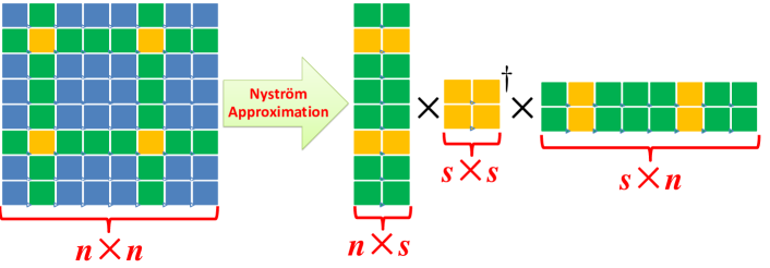
Figure 6.1: The illustration of the Nyström method.

There are a few things to remark:

• The Nyström is highly efficient. When applied to speedup kernel methods, the scalability can be as large as $n=10^{6}$.

• The Nyström method is a rough approximation to ${\bf K}$ and is well known to be of low accuracy. If a moderately high accuracy is required, one had better use the method in the previous section.

• The $s\times s$ matrix ${\bf W}$ is usually ill-conditioned, and thus the Moore-Penrose inverse can be numerically instable. (It is because the bottom singular values of ${\bf W}$ blow up during the Moore-Penrose inverse.) A very effective heuristic is to drop the bottom singular values of ${\bf W}$: set a parameter $k<s$, e.g. $k=\lceil 0.8s\rceil$, and approximate ${\bf K}$ by ${\bf C}({\bf W}_{k})^{\dagger}{\bf C}^{T}$.

• There are many choices of the sampling matrix ${\bf S}$. See [13] for more discussions.

The Nyström method can be implemented in $11$ lines of MATLAB code. The output of the algorithm is ${\bf L}\in{\mathbb{R}}^{n\times k}$, where ${\bf L}{\bf L}^{T}$ is the Nyström approximation to ${\bf K}$.

⬇

1function [L] = Nystrom(X, sigma, s)

2k = ceil(0.8 * s); % can be tuned

3n = size(X, 1);

4S = sort(randsample(n, s)); % uniform sampling

5C = rbf(X, X(S, :), sigma); % C = K(:, S)

6W = C(S, :);

7[UW, SW, ~] = svd(W);

8SW = diag(SW);

9SW = 1 ./ sqrt(SW(1:k));

10UW = bsxfun(@times, UW(:, 1:k), SW’);

11L = C * UW; % K is approximated by L * L’

Here we use the RBF kernel function implemented in Section 6.1. Line 8 sets $k=\lceil 0.8c\rceil$, which can be better tuned to enhance numerical stability. Notice that $k$ should not be set too small, otherwise the accuracy would be affected.

6.5 More Efficient Extensions

Several SPSD matrix approximation methods has been proposed recently, and they are more scalable than the Nyström method in certain applications. This section briefly describes some of these methods.

6.5.1 Memory Efficient Kernel Approximation (MEKA)

MEKA [24] exploits the block structure of kernel matrices and is more memory efficient than the Nyström method. MEKA first partitions the data ${\bf x}_{1},\cdots,{\bf x}_{n}$ into $b$ groups (e.g. by inexact $k$means clustering), accordingly, the kernel matrix ${\bf K}$ has $b\times b$ blocks:

$${\bf K}\;=\;\left[\begin{array}[]{ccc}{\bf K}_{[1,1]}&\cdots&{\bf K}_{[1,b]}\\ \vdots&\ddots&\vdots\\ {\bf K}_{[b,1]}&\cdots&{\bf K}_{[b,b]}\\ \end{array}\right]\;=\;\left[\begin{array}[]{c}{\bf K}_{[1:]}\\ \vdots\\ {\bf K}_{[b:]}\\ \end{array}\right].$$

Then MEKA approximately computes the top left singular vectors of ${\bf K}_{[1:]},\cdots,{\bf K}_{[b:]}$, denote ${\bf U}_{[1]}$, $\cdots,{\bf U}_{[b]}$, respectively. For each $(i,j)\in[b]\times[b]$, MEKA finds a very small-scale matrix ${\bf Z}_{[i,j]}$ by solving

$${\bf Z}_{[i,j]}\;=\;\mathop{\rm argmin}_{\bf Z}\big{\|}{\bf K}_{[i,j]}-{\bf U}_{[i]}{\bf Z}_{[i,j]}{\bf U}_{[j]}^{T}\big{\|}_{F}^{2}.$$

This can be done efficiently using the approach in Section 4.5. Finally, the low-rank approximation is

$${\bf K}\;\approx\;\left[\begin{array}[]{ccc}{\bf U}_{[1]}&&{\bf 0}\\ &\ddots&\\ {\bf 0}&&{\bf U}_{[b]}\\ \end{array}\right]\left[\begin{array}[]{ccc}{\bf Z}_{[1,1]}&\cdots&{\bf Z}_{[1,b]}\\ \vdots&\ddots&\vdots\\ {\bf Z}_{[b,1]}&\cdots&{\bf Z}_{[b,b]}\\ \end{array}\right]\left[\begin{array}[]{ccc}{\bf U}_{[1]}&&{\bf 0}\\ &\ddots&\\ {\bf 0}&&{\bf U}_{[b]}\\ \end{array}\right]^{T}\;=\;{\bf U}{\bf Z}{\bf U}^{T}.$$

Since ${\bf Z}$ and ${\bf U}_{[1]},\cdots,{\bf U}_{[b]}$ are small-scale matrices, MEKA is thus very memory efficient. There are several things to remark:

• MEKA can be used to speedup Gaussian process regression and least squares SVM. However, MEKA can be hardly applied to speedup $k$-eigenvalue decomposition, because it requires the $k$-SVD of ${\bf U}{\bf Z}^{1/2}$, which destroys the sparsity and significantly increases memory cost.

• Indiscreet implementation, e.g. the implementation provided by [24], can make MEKA numerically unstable, as was reported by [30; 28]. The readers had better to follow the stabler implementation in [28].

6.5.2 Structured Kernel Interpolation (SKI)

SKI [33] is a memory efficient extension of the Nyström method. Let ${\bf S}$ be a column selection matrix, ${\bf C}={\bf K}{\bf S}$, and ${\bf W}={\bf S}^{T}{\bf C}={\bf S}^{T}{\bf K}{\bf S}$. The Nyström method approximates ${\bf K}$ by ${\bf C}{\bf W}^{\dagger}{\bf C}^{T}$. SKI further approximates each row of ${\bf C}$ by a convex combination of two rows of ${\bf W}$ and obtain ${\bf C}\approx{\bf X}{\bf W}$. Notice that each row of ${\bf X}$ has only two nonzero entries, which makes ${\bf X}$ extremely sparse. In this way, ${\bf K}$ is approximated by

$${\bf K}\;\approx\;{\bf C}{\bf W}^{\dagger}{\bf C}\;\approx\;({\bf X}{\bf W}){\bf W}^{\dagger}({\bf X}{\bf W})^{T}\;=\;{\bf X}{\bf W}{\bf X}^{T}.$$

Much accuracy is lost in the second approximation, so SKI is much less accurate than the Nyström method. For the same reason as MEKA, there is no point in applying SKI to speedup $k$-eigenvalue decomposition of ${\bf K}$.

6.6 Extension to Rectangular Matrices: CUR Matrix Decomposition

This section considers the problem of sketching any rectangular matrix ${\bf A}$ by the CUR matrix decomposition [16]. The CUR matrix decomposition is an extension of the previously discussed SPSD matrix sketching methods.

6.6.1 Motivation

Suppose we are given $n$ training data ${\bf x}_{1},\cdots,{\bf x}_{n}\in{\mathbb{R}}^{d}$, $m$ test data ${\bf x}_{1}^{\prime},\cdots,{\bf x}_{m}^{\prime}\in{\mathbb{R}}^{d}$, and a kernel function $\kappa(\cdot,\cdot)$. In their generalization (test) stage, kernel methods such as GPR and KPCA form an $m\times n$ matrix ${\bf K}_{*}$, where $({\bf K}_{*})_{ij}=\kappa({\bf x}_{i}^{\prime},{\bf x}_{j})$, and apply ${\bf K}_{*}$ to some vectors or matrices. Notice that it takes ${\mathcal{O}}(mnd)$ time to form ${\bf K}_{*}$ and ${\mathcal{O}}(mnp)$ time to multiply ${\bf K}_{*}$ by an $n\times p$ matrix. If $m$ is as large as $n$, the generalization stage of such kernel methods can be very expensive. Fortunately, with the help of the CUR matrix decomposition, the generalization stage of GPR or KPCA merely costs time linear in $m+n$.

6.6.2 Prototype CUR Decomposition

Suppose we are given an arbitrary $m\times n$ rectangular matrix ${\bf A}$, which can be the aforementioned ${\bf K}_{*}$. We sample $c$ columns of ${\bf A}$ to form ${\bf C}={\bf A}{\bf S}_{\bf C}\in{\mathbb{R}}^{m\times c}$, sample $r$ rows of ${\bf A}$ to form ${\bf R}={\bf A}{\bf S}_{\bf R}\in{\mathbb{R}}^{r\times n}$, and compute the intersection matrix ${\bf U}^{\star}\in{\mathbb{R}}^{c\times r}$ by solving

$${\bf U}^{\star}\;=\;\mathop{\rm argmin}_{{\bf U}}\|\underbrace{{\bf A}}_{m\times n}-\underbrace{{\bf C}}_{m\times c}\underbrace{{\bf U}}_{c\times r}\underbrace{{\bf R}}_{r\times n}\|_{F}^{2}\;=\;{\bf C}^{\dagger}{\bf A}{\bf R}^{\dagger}.$$ (6.3)

The approximation ${\bf A}\approx{\bf C}{\bf U}^{\star}{\bf R}$ is well known as the CUR decomposition [16]. This formulation bears a strong resemblance with the prototype SPSD matrix sketching method in (6.1).

The prototype CUR decomposition is not very useful because (1) its time cost is ${\mathcal{O}}(mn\cdot\min\{c,r\})$ and (2) it visits every entry of ${\bf A}$.

6.6.3 Faster CUR Decomposition

Analogous to the SPSD matrix sketching, we can compute ${\bf U}^{\star}$ approximately and significantly more efficiently. Let ${\bf P}_{\bf C}\in{\mathbb{R}}^{m\times p_{c}}$ and ${\bf P}_{\bf R}\in{\mathbb{R}}^{n\times p_{r}}$ be some column selection matrices. Then we solve this problem in stead of (6.3):

$$\tilde{\bf U}\;=\;\mathop{\rm argmin}_{{\bf U}}\|\underbrace{{\bf P}_{\bf C}^{T}{\bf A}{\bf P}_{\bf R}}_{p_{c}\times p_{r}}-\underbrace{{\bf P}_{\bf C}^{T}{\bf C}}_{p_{c}\times c}\underbrace{{\bf U}}_{c\times r}\underbrace{{\bf R}{\bf P}_{\bf R}}_{r\times p_{r}}\|_{F}^{2}\;=\;({\bf P}_{\bf C}^{T}{\bf C})^{\dagger}({\bf P}_{\bf C}^{T}{\bf A}{\bf P}_{\bf R})({\bf R}{\bf P}_{\bf R})^{\dagger}.$$ (6.4)

The faster CUR decomposition is very similar to the faster SPSD matrix sketching method in Section 6.3. The faster CUR decomposition has the following properties:

• It visits only $mc+nr+p_{c}p_{r}$ entries of ${\bf A}$, which is linear in $m+n$. This is particularly useful when applied to kernel methods, because it avoids forming the whole kernel matrix.

• The overall time and memory costs are linear in $m+n$.

• If ${\bf P}_{\bf C}$ is the leverage score sampling matrix corresponding to the columns of ${\bf C}^{T}$ and ${\bf P}_{\bf R}$ is the leverage score sampling matrix corresponding to the columns of ${\bf R}$, then $\tilde{\bf U}$ is a very high quality approximation to ${\bf U}^{\star}$ [31]:

  $$\|{\bf A}-{\bf C}\tilde{\bf U}{\bf R}\|_{F}^{2}\;\leq\;(1+\epsilon)\min_{\bf U}\|{\bf A}-{\bf C}{\bf U}{\bf R}\|_{F}^{2}$$

  holds with high probability.

Empirically speaking, setting ${\bf P}_{\bf C}$ and ${\bf P}_{\bf R}$ be uniform sampling matrices works nearly as well as leverage score sampling matrices, and setting $p_{c}=p_{r}={\mathcal{O}}(c+r)$ suffices for a high approximation quality. If ${\bf A}$ is a full-observed matrix, the CUR matrix decomposition can be computed by the following MATLAB code.

⬇

1function [C, U, R] = curFaster(A, c, r)

2pc = 2 * (r + c); % can be tuned

3pr = 2 * (r + c); % can be tuned

4[m, n] = size(A);

5SC = sort(randsample(n, c));

6SR = sort(randsample(m, r));

7C = A(:, SC);

8R = A(SR, :);

9PC = sort(randsample(m, pc));

10PR = sort(randsample(n, pr));

11PC = unique([PC; SR]); % enforce PC to contain SR

12PR = unique([PR; SC]); % enforce PR to contain SC

13U = pinv(C(PC, :)) * A(PC, PR) * pinv(R(:, PR));

Let’s consider the kernel approximation problem in Section 6.6.1. Let ${\bf X}_{\textrm{train}}\in{\mathbb{R}}^{n\times d}$ be the training data and ${\bf X}_{\textrm{test}}\in{\mathbb{R}}^{m\times d}$ be the test data. We use the RBF kernel with kernel width parameter $\sigma$. The $m\times n$ matrix ${\bf K}_{*}$ can be approximated by $\tilde{\bf K}_{*}={\bf C}{\bf U}{\bf R}$, which is the output of the following MATLAB procedure.

⬇

1function [C, U, R] = curFasterKernel(Xtest, Xtrain, sigma, c, r)

2pc = 2 * (r + c); % can be tuned

3pr = 2 * (r + c); % can be tuned

4m = size(Xtest, 1);

5n = size(Xtrain, 1);

6SC = sort(randsample(n, c));

7SR = sort(randsample(m, r));

8C = rbf(Xtest, Xtrain(SC, :), sigma);

9R = rbf(Xtest(SR, :), Xtrain, sigma);

10PC = sort(randsample(m, pc));

11PR = sort(randsample(n, pr));

12PC = unique([PC; SR]); % enforce PC to contain SR

13PR = unique([PR; SC]); % enforce PR to contain SC

14Kblock = rbf(Xtest(PC, :), Xtrain(PR, :), sigma);

15U = pinv(C(PC, :)) * Kblock * pinv(R(:, PR));

The time cost of this procedure is linear in $m+n$, and $\tilde{\bf K}_{*}={\bf C}{\bf U}{\bf R}$ can be applied to $n$ dimensional vector in ${\mathcal{O}}\big{(}nr+mc)$ time. In this way, the generalization of GPR and KPCA can be efficient.

6.7 Applications

This section provides the implementations of kernel PCA, spectral clustering, Gaussian process regression, all sped-up by randomized algorithms.

6.7.1 Kernel Principal Component Analysis (KPCA)

Suppose we are given

• $n$ training data ${\bf x}_{1},\cdots,{\bf x}_{n}\in{\mathbb{R}}^{d}$,

• $m$ test data ${\bf x}_{1}^{\prime},\cdots,{\bf x}_{m}^{\prime}\in{\mathbb{R}}^{d}$, (${\bf x}_{i}^{\prime}$ is not the transpose ${\bf x}_{i}^{T}$),

• a kernel function $\kappa(\cdot,\cdot)$, e.g. the RBF kernel function,

• a target rank $k$ ($\ll n,d$).

The goal of KPCA is to extract $k$ features of each training datum and each test datum, which may be used in clustering or classification. The standard KPCA consists of the following steps:

1. Training

   1. Form the $n\times n$ kernel matrix ${\bf K}$ of the training data, whose the $(i,j)$-th entry is $\kappa({\bf x}_{i},{\bf x}_{j})$;

   2. Compute the $k$-eigenvalue decomposition ${\bf K}_{k}={\bf U}_{k}\mbox{\boldmath$\Lambda$\unboldmath}_{k}{\bf U}_{k}^{T}$;

   3. Form the $n\times k$ matrix ${\bf U}_{k}\mbox{\boldmath$\Lambda$\unboldmath}_{k}^{1/2}$, whose the $i$-th row is the feature of ${\bf x}_{i}$;

2. Generalization (test)

   1. Form the $m\times n$ kernel matrix ${\bf K}_{*}$ whose the $(i,j)$-th entry is $\kappa({\bf x}_{i}^{\prime},{\bf x}_{j})$;

   2. Form the $m\times k$ matrix ${\bf K}_{*}{\bf U}_{k}\mbox{\boldmath$\Lambda$\unboldmath}_{k}^{-1/2}$, whose the $i$-th row is the feature of ${\bf x}_{i}^{\prime}$.

The most time and memory expensive step in training is the $k$-eigenvalue decomposition of ${\bf K}$, which can be sped-up by the sketching techniques discussed in this section. Empirically, the faster SPSD matrix sketching in Section 6.3 is much more accurate than the Nyström method in Section 6.4, and their time and memory costs are all linear in $n$. Thus the faster SPSD matrix sketching can be better choice. KPCA can be approximately solved by several lines of MATLAB code.

⬇

1function [U, lambda, featuretrain] = kpcaTrain(Xtrain, sigma, k)

2s = k * 10; % can be tuned

3[QC, Z] = spsdFaster(Xtrain, sigma, s); % QC has orthogonal columns

4clear Xtrain

5[UZ, SZ, ~] = svd(Z);

6U = QC * UZ(:, 1:k); % U contains the top k eigenvectors

7lambda = diag(SZ);

8lambda = lambda(1:k); % lambda is the vector containing the top k eigenvalues

9featuretrain = bsxfun(@times, U, (sqrt(lambda))’);

10end

⬇

1function [featuretest] = kpcaTest(Xtrain, Xtest, sigma, U, lambda)

2Ktest = rbf(Xtest, Xtrain, sigma);

3U = bsxfun(@times, U, (1 ./ sqrt(lambda))’);

4featuretest = Ktest * U;

5end

In the function “$\mathrm{kpcaTrain}$”, the input variable “$\mathrm{Xtrain}$” has $n$ rows, each of which corresponds to a training datum. The rows of the output “$\mathrm{featuretrain}$” and “$\mathrm{featuretest}$” are the features extracted by KPCA, and the features can be used to perform classification. For example, suppose each datum ${\bf x}_{i}$ is associated with a label $y_{i}$, and let ${\bf y}=[y_{1},\cdots,y_{n}]^{T}\in{\mathbb{R}}^{n}$. We can use $k$-nearest-neighbor

⬇

1[ytest] = knnclassify(featuretest, featuretrain, y)

to predict the labels of the test data.

When the number of test data $m$ is large, the function “kpcaTest” is costly. The users should apply the CUR decomposition in Section 6.6.3 to speedup computation.

⬇

1function [featuretest] = kpcaTestCUR(Xtrain, Xtest, sigma, U, lambda)

2c = max(100, ceil(size(Xtrain, 1) / 20)); % can be tuned

3r = max(100, ceil(size(Xtest, 1) / 20)); % can be tuned

4[C, Utilde, R] = curFasterKernel(Xtest, Xtrain, sigma, c, r);

5U = bsxfun(@times, U, (1 ./ sqrt(lambda))’);

6featuretest = C * (Utilde * (R * U));

7end

6.7.2 Spectral Clustering

Spectral clustering is one of the most popular clustering algorithms. Suppose we are given

• $n$ data points ${\bf x}_{1},\cdots,{\bf x}_{n}\in{\mathbb{R}}^{d}$,

• a kernel function $\kappa(\cdot,\cdot)$,

• $k$: the number of classes.

Spectral clustering performs the following operations:

1. Form an $n\times n$ kernel matrix ${\bf K}$, where big $k_{ij}$ indicates ${\bf x}_{i}$ and ${\bf x}_{j}$ are similar;

2. Form the degree matrix ${\bf D}$ with $d_{ii}=\sum_{j}k_{ij}$ and $d_{ij}=0$ for all $i\neq j$;

3. Compute the normalized graph Laplacian ${\bf G}={\bf D}^{-1/2}{\bf K}{\bf D}^{-1/2}\in{\mathbb{R}}^{n\times n}$;

4. Compute the top $k$ eigenvectors of ${\bf G}$, denote ${\bf U}\in{\mathbb{R}}^{n\times k}$, and normalize the rows of ${\bf U}$;

5. Apply $k$means clustering on the rows of ${\bf V}$ to obtain the class labels.

The first step costs ${\mathcal{O}}(n^{2}d)$ time and the fourth step costs ${\mathcal{O}}(n^{2}k)$ times, which limit the scalability of spectral clustering. Fowlkes et al. [11] proposed to apply the Nyström method to make spectral clustering more scalable by avoiding forming the whole kernel matrix and speeding-up the $k$-eigenvalue decomposition. Empirically, the algorithm in Section 6.3 is more accurate than the Nyström method in Section 6.4, and they both runs in linear time. Spectral clustering with the randomized algorithm in Section 6.3 can be implemented in 16 lines of MATLAB code.

⬇

1function [labels] = SpectralClusteringFaster(X, sigma, k)

2s = k * 10; % can be tuned

3n = size(X, 1);

4[QC, Z] = spsdFaster(X, sigma, s); % K is approximated by QC * Z * QC’

5[UZ, SZ, ~] = svd(Z);

6SZ = sqrt(diag(SZ));

7UZ = bsxfun(@times, UZ, SZ’); % now Z = UZ * UZ’

8L = QC * UZ; % now K is approximated by L * L’

9d = ones(n, 1);

10d = L * (L’ * d); % diagonal of the degree matrix D

11d = 1 ./ sqrt(d);

12L = bsxfun(@times, L, d); % now G is approximated by L*L’

13[U, ~, ~] = svd(L, ’econ’);

14U = U(:, 1:k);

15U = normr(U); % normalize the rows of U

16labels = kmeans(U, k, ’Replicates’, 3);

When the scale of data is too large for the faster SPSD matrix sketching algorithm in Section 6.3, one can instead use the more efficient Nyström method in Section 6.4: simply replace Lines 4 to 8 by

⬇

1L = Nystrom(X, sigma, s);

6.7.3 Gaussian Process Regression (GPR)

The Gaussian process regression (GPR) is one of the most popular machine learning methods. GPR is the foundation of Bayesian optimization and has important applications such as automatically tuning the hyper-parameters of deep neural networks. Suppose we are given

• $n$ training data ${\bf x}_{1},\cdots,{\bf x}_{n}\in{\bf R}^{d}$,

• labels ${\bf y}=[y_{1},\cdots y_{n}]^{T}\in{\mathbb{R}}^{n}$ of the training data,

• $m$ test data ${\bf x}_{1}^{\prime},\cdots,{\bf x}_{m}^{\prime}\in{\mathbb{R}}^{d}$, (${\bf x}_{i}^{\prime}$ is not the transpose ${\bf x}_{i}^{T}$),

• and a kernel function $\kappa(\cdot,\cdot)$, e.g. the RBF kernel with kernel width parameter $\sigma$.

Training. In the training stage, GPR requires forming the $n\times n$ kernel matrix ${\bf K}$ where $k_{ij}=\kappa({\bf x}_{i},{\bf x}_{j})$ and computing the model

$${\bf w}\;=\;({\bf K}+\alpha{\bf I}_{n})^{-1}{\bf y}.$$

Here $\alpha$ is a tuning parameter that indicates the noise intensity in the labels ${\bf y}$. It takes ${\mathcal{O}}(n^{2}d)$ time to form the kernel matrix and ${\mathcal{O}}(n^{3})$ time to compute the matrix inversion. To make the training efficient, we can first sketch the SPSD matrix ${\bf K}$ to obtain ${\bf K}\approx{\bf L}{\bf L}^{T}$ and then apply the technique in Section 6.1.2 to obtain ${\bf w}$. Empirically, when applied to speedup GPR, the algorithms discussed in Section 6.3 and Section 6.4 has similar accuracy, thus we choose to use the Nyström method which is more efficient.

The training GPR with the Nyström approximation can be implemented in the following MATLAB code. The time cost is ${\mathcal{O}}(nl^{2}+nld)$ and the space cost is ${\mathcal{O}}(nl+nd)$.

⬇

1function [w] = gprTrain(Xtrain, ytrain, sigma, alpha)

2l = 100; % can be tuned

3L = Nystrom(Xtrain, sigma, l); % K is approximated by L * L’

4l = size(L, 2);

5w = L’ * ytrain;

6w = (alpha * eye(l) + L’ * L) \ w;

7w = ytrain - L * w;

8w = w / alpha;

9end

The input “$\mathrm{sigma}$” is the kernel width parameter and “$\mathrm{alpha}$” indicates the noise intensity in the observation.

Generalization (test). After obtaining the trained model ${\bf w}\in{\mathbb{R}}^{n}$, GPR can predict the unknown labels of the $m$ test data ${\bf x}_{1}^{\prime},\cdots,{\bf x}_{m}^{\prime}\in{\mathbb{R}}^{d}$. GPR forms an $m\times n$ kernel matrix ${\bf K}_{*}$ whose the $(i,j)$-th entry is $\kappa({\bf x}_{i}^{\prime},{\bf x}_{j})$ and compute ${\bf y}_{*}={\bf K}_{*}{\bf w}\in{\mathbb{R}}^{m}$. The $i$-th entry in ${\bf y}_{*}$ is the predictive label of ${\bf x}_{i}^{\prime}$. The generalization can be implemented in four lines of MATLAB code.

⬇

1function [ytest] = gprTest(Xtrain, Xtest, sigma, w)

2Ktest = rbf(Xtest, Xtrain, sigma);

3ytest = Ktest * w;

4end

It costs ${\mathcal{O}}(mnd)$ time to compute ${\bf K}_{*}$ and ${\mathcal{O}}(mn)$ time to apply ${\bf K}_{*}$ to ${\bf w}$. If $m$ is small, the generalization stage can be performed straightforwardly. However, if $m$ is as large as $n$, the time cost will be quadratic in $n$, and the user should apply the CUR decomposition in Section 6.6.3 to speedup computation.

⬇

1function [ytest] = gprTestCUR(Xtrain, Xtest, sigma, w)

2c = max(100, ceil(size(Xtrain, 1) / 20)); % can be tuned

3r = max(100, ceil(size(Xtest, 1) / 20)); % can be tuned

4[C, Utilde, R] = curFasterKernel(Xtest, Xtrain, sigma, c, r);

5ytest = C * (Utilde * (R * w));

6end

Appendix A Several Facts of Matrix Algebra

This chapter lists some facts that has been applied in this paper.

Fact A.1.

The matrices ${\bf Q}_{1}\in{\mathbb{R}}^{m\times n}$ and ${\bf Q}_{n\times p}$ ($m\geq n\geq p$) have orthonormal columns. Then the matrix ${\bf Q}={\bf Q}_{1}{\bf Q}_{2}$ has orthonormal columns.

Fact A.2.

Let ${\bf A}$ be any $m\times n$ and rank $\rho$ matrix. Then ${\bf A}{\bf A}^{\dagger}{\bf B}={\bf U}_{\bf A}{\bf U}_{\bf A}^{T}{\bf B}={\bf A}{\bf X}^{\star}={\bf U}_{\bf A}{\bf Z}^{\star},$ where

$${\bf X}^{\star}\;=\;\mathop{\rm argmin}_{\bf X}\|{\bf B}-{\bf A}{\bf X}\|_{F}^{2},\qquad\textrm{ and }\qquad{\bf Z}^{\star}\;=\;\mathop{\rm argmin}_{\bf Z}\|{\bf B}-{\bf U}_{\bf A}{\bf Z}\|_{F}^{2}.$$

This is the reason why ${\bf A}{\bf A}^{\dagger}{\bf B}$ and ${\bf U}_{\bf A}{\bf U}_{\bf A}^{T}{\bf B}$ are called the projection of ${\bf B}$ onto the column space of ${\bf A}$.

Fact A.3.

[34, Lemma 44] The matrices ${\bf Q}\in{\mathbb{R}}^{m\times s}$ ($m\geq s$) has orthonormal columns. The solution to

$$\mathop{\rm argmin}_{\mathrm{rank}({\bf X})\leq k}\|{\bf A}-{\bf Q}{\bf X}\|_{F}^{2}$$

is ${\bf X}^{\star}=({\bf Q}^{T}{\bf A})_{k}$, where $({\bf Q}^{T}{\bf A})_{k}$ denotes the closest rank $k$ approximation to ${\bf Q}^{T}{\bf A}$.

Fact A.4.

Let ${\bf A}^{\dagger}$ be the Moore-Penrose inverse of ${\bf A}$. Then ${\bf A}{\bf A}^{\dagger}{\bf A}={\bf A}$ and ${\bf A}^{\dagger}{\bf A}{\bf A}^{\dagger}={\bf A}^{\dagger}$.

Fact A.5.

Let ${\bf A}$ be an $m\times n$ ($m\geq n$) matrix and ${\bf A}={\bf Q}_{\bf A}{\bf R}_{\bf A}$ be the QR decomposition of ${\bf A}$. Then

$$\underbrace{{\bf A}^{\dagger}}_{n\times m}\;=\;\underbrace{{\bf R}_{\bf A}^{\dagger}}_{n\times n}\underbrace{{\bf Q}_{\bf A}^{T}}_{n\times m}.$$

Fact A.6.

Let ${\bf C}$ be a full-rank matrix with more rows than columns. Let ${\bf C}={\bf Q}_{\bf C}{\bf R}_{\bf C}$ be the QR decomposition and ${\bf C}={\bf U}_{\bf C}\mbox{\boldmath$\Sigma$\unboldmath}_{\bf C}{\bf V}_{\bf C}$ be the condensed SVD. Then the leverage scores of ${\bf C}$, ${\bf Q}_{\bf C}$, ${\bf U}_{\bf C}$ are the same.

Appendix B Notes and Further Reading

The $\ell_{p}$ Regression Problems. Chapter 4 has applied the sketching methods to solve the $\ell_{2}$ norm regression problem more efficiently. The more general $\ell_{p}$ regression problems have also been studied in the literature [5; 7; 17; 8]. Especially, the $\ell_{1}$ is of great interest because it demonstrate strong robustness to noise. Currently the strongest result is the $\ell_{p}$ row sampling by Lewis weights [8].

Distributed SVD. In the distributed model, each machine holds a subset of columns of ${\bf A}$, and the system outputs the top singular values and singular vectors. In this model, the communication cost should also be considered, as well as the time and memory costs. The seminal work [10] proposed to build a coreset to capture the properties of ${\bf A}$, which facilitates low computation and communication costs. Later on, several algorithms with stronger error bound and lower communication and computation costs have been proposed. Currently, the state of the art is [2].

Random Feature for Kernel Methods. Chapter 6 has introduced the sketching methods for kernel methods. A parallel line of work is the random feature methods [22] which also form low-rank approximations to kernel matrices. Section 6.5.3 of [27] offers simple and elegant proof of a random feature method. Since the sketching methods usually works better than the random feature methods (see the examples in [35]), the users are advised to apply the sketching methods introduced in Chapter 6. Besides the two kinds of low-rank approximation approaches, the stochastic optimization approach [9] also demonstrates very high scalability.

References

- Ben-Israel and Greville [2003] Adi Ben-Israel and Thomas N.E. Greville. Generalized Inverses: Theory and Applications. Second Edition. Springer, 2003.
- Boutsidis and Woodruff [2015] Christos Boutsidis and David P Woodruff. Communication-optimal distributed principal component analysis in the column-partition model. arXiv preprint arXiv:1504.06729, 2015.
- Boutsidis et al. [2014] Christos Boutsidis, Petros Drineas, and Malik Magdon-Ismail. Near-optimal column-based matrix reconstruction. SIAM Journal on Computing, 43(2):687–717, 2014.
- Charikar et al. [2004] Moses Charikar, Kevin Chen, and Martin Farach-Colton. Finding frequent items in data streams. Theoretical Computer Science, 312(1):3–15, 2004.
- Clarkson [2005] Kenneth L Clarkson. Subgradient and sampling algorithms for l1 regression. In Proceedings of the sixteenth annual ACM-SIAM symposium on Discrete algorithms, pages 257–266. Society for Industrial and Applied Mathematics, 2005.
- Clarkson and Woodruff [2013] Kenneth L. Clarkson and David P. Woodruff. Low rank approximation and regression in input sparsity time. In Annual ACM Symposium on theory of computing (STOC). ACM, 2013.
- Clarkson et al. [2013] Kenneth L Clarkson, Petros Drineas, Malik Magdon-Ismail, Michael W Mahoney, Xiangrui Meng, and David P Woodruff. The fast cauchy transform and faster robust linear regression. In Proceedings of the Twenty-Fourth Annual ACM-SIAM Symposium on Discrete Algorithms, pages 466–477. SIAM, 2013.
- Cohen and Peng [2014] Michael B Cohen and Richard Peng. row sampling by lewis weights. arXiv preprint arXiv:1412.0588, 2014.
- Dai et al. [2014] Bo Dai, Bo Xie, Niao He, Yingyu Liang, Anant Raj, Maria-Florina F Balcan, and Le Song. Scalable kernel methods via doubly stochastic gradients. In Advances in Neural Information Processing Systems (NIPS). 2014.
- Feldman et al. [2013] Dan Feldman, Melanie Schmidt, and Christian Sohler. Turning big data into tiny data: Constant-size coresets for k-means, pca and projective clustering. In Proceedings of the Twenty-Fourth Annual ACM-SIAM Symposium on Discrete Algorithms, pages 1434–1453. SIAM, 2013.
- Fowlkes et al. [2004] Charless Fowlkes, Serge Belongie, Fan Chung, and Jitendra Malik. Spectral grouping using the Nyström method. IEEE Transactions on Pattern Analysis and Machine Intelligence, 26(2):214–225, 2004.
- Gittens [2011] Alex Gittens. The spectral norm error of the naive Nyström extension. arXiv preprint arXiv:1110.5305, 2011.
- Gittens and Mahoney [2013] Alex Gittens and Michael W. Mahoney. Revisiting the nyström method for improved large-scale machine learning. In International Conference on Machine Learning (ICML), 2013.
- Halko et al. [2011] Nathan Halko, Per-Gunnar Martinsson, and Joel A. Tropp. Finding structure with randomness: Probabilistic algorithms for constructing approximate matrix decompositions. SIAM Review, 53(2):217–288, 2011.
- Johnson and Lindenstrauss [1984] William B. Johnson and Joram Lindenstrauss. Extensions of Lipschitz mappings into a Hilbert space. Contemporary mathematics, 26(189-206), 1984.
- Mahoney [2011] Michael W. Mahoney. Randomized algorithms for matrices and data. Foundations and Trends in Machine Learning, 3(2):123–224, 2011.
- Meng and Mahoney [2013] Xiangrui Meng and Michael W Mahoney. Low-distortion subspace embeddings in input-sparsity time and applications to robust linear regression. In Proceedings of the forty-fifth annual ACM symposium on theory of computing, pages 91–100. ACM, 2013.
- Meng et al. [2014] Xiangrui Meng, Michael A Saunders, and Michael W Mahoney. Lsrn: A parallel iterative solver for strongly over-or underdetermined systems. SIAM Journal on Scientific Computing, 36(2):C95–C118, 2014.
- Musco and Musco [2015] Cameron Musco and Christopher Musco. Stronger approximate singular value decomposition via the block Lanczos and power methods. Advances in Neural Information Processing Systems (NIPS), 2015.
- Nyström [1930] Evert J. Nyström. Über die praktische auflösung von integralgleichungen mit anwendungen auf randwertaufgaben. Acta Mathematica, 54(1):185–204, 1930.
- Pham and Pagh [2013] Ninh Pham and Rasmus Pagh. Fast and scalable polynomial kernels via explicit feature maps. In the 19th ACM SIGKDD international conference on Knowledge discovery and data mining (KDD), pages 239–247. ACM, 2013.
- Rahimi and Recht [2007] Ali Rahimi and Benjamin Recht. Random features for large-scale kernel machines. In Advances in neural information processing systems (NIPS), pages 1177–1184, 2007.
- Saad [2011] Yousef Saad. Numerical methods for large eigenvalue problems. preparation. Available from: http://www-users. cs. umn. edu/saad/books. html, 2011.
- Si et al. [2014] Si Si, Cho-Jui Hsieh, and Inderjit Dhillon. Memory efficient kernel approximation. In International Conference on Machine Learning (ICML), pages 701–709, 2014.
- Stewart [1999] G. W. Stewart. Four algorithms for the efficient computation of truncated pivoted QR approximations to a sparse matrix. Numerische Mathematik, 83(2):313–323, 1999.
- Thorup and Zhang [2012] Mikkel Thorup and Yin Zhang. Tabulation-based 5-independent hashing with applications to linear probing and second moment estimation. SIAM J. Comput., 41(2):293–331, April 2012. ISSN 0097-5397.
- Tropp [2015] Joel A Tropp. An introduction to matrix concentration inequalities. arXiv preprint arXiv:1501.01571, 2015.
- Wang et al. [2015a] Ruoxi Wang, Yingzhou Li, Michael W Mahoney, and Eric Darve. Structured block basis factorization for scalable kernel matrix evaluation. arXiv preprint arXiv:1505.00398, 2015a.
- Wang and Zhang [2013] Shusen Wang and Zhihua Zhang. Improving CUR matrix decomposition and the Nyström approximation via adaptive sampling. Journal of Machine Learning Research, 14:2729–2769, 2013.
- Wang et al. [2014] Shusen Wang, Luo Luo, and Zhihua Zhang. Spsd matrix approximation via column selection: Theories, algorithms, and extensions. CoRR, abs/1406.5675, 2014.
- Wang et al. [2015b] Shusen Wang, Zhihua Zhang, and Tong Zhang. Towards more efficient symmetric matrix sketching and CUR matrix decomposition. arXiv preprint arXiv:1503.08395, 2015b.
- Williams and Seeger [2001] Christopher Williams and Matthias Seeger. Using the Nyström method to speed up kernel machines. In Advances in Neural Information Processing Systems (NIPS), 2001.
- Wilson and Nickisch [2015] Andrew Gordon Wilson and Hannes Nickisch. Kernel interpolation for scalable structured gaussian processes (kiss-gp). arXiv preprint arXiv:1503.01057, 2015.
- Woodruff [2014] David P Woodruff. Sketching as a tool for numerical linear algebra. arXiv preprint arXiv:1411.4357, 2014.
- Yang et al. [2012] Tianbao Yang, Yu-Feng Li, Mehrdad Mahdavi, Rong Jin, and Zhi-Hua Zhou. Nyström method vs random fourier features: A theoretical and empirical comparison. In Advances in Neural Information Processing Systems (NIPS), 2012.
- Zhang and Kwok [2010] Kai Zhang and James T. Kwok. Clustered Nyström method for large scale manifold learning and dimension reduction. IEEE Transactions on Neural Networks, 21(10):1576–1587, 2010.