The Cosmic Dawn and Epoch of Reionization with the Square Kilometre Array

Abstract:

Concerted effort is currently ongoing to open up the Epoch of Reionization ($z\sim$15-6) for studies with IR and radio telescopes. Whereas IR detections have been made of sources (Lyman-$\alpha$ emitters, quasars and drop-outs) in this redshift regime in relatively small fields of view, no direct detection of neutral hydrogen, via the redshifted 21-cm line, has yet been established. Such a direct detection is expected in the coming years, with ongoing surveys, and could open up the entire universe from $z\sim$6-200 for astrophysical and cosmological studies, opening not only the Epoch of Reionization, but also its preceding Cosmic Dawn ($z\sim$30-15) and possibly even the later phases of the Dark Ages ($z\sim$200-30). All currently ongoing experiments attempt statistical detections of the 21-cm signal during the Epoch of Reionization, with limited signal-to-noise. Direct imaging, except maybe on the largest (degree) scales at lower redshifts, as well as higher redshifts will remain out of reach. The Square Kilometre Array (SKA) will revolutionize the field, allowing direct imaging of neutral hydrogen from scales of arc-minutes to degrees over most of the redshift range $z\sim$6-28 with SKA1-LOW, and possibly even higher redshifts with the SKA2-LOW. In this SKA will be unique, and in parallel provide enormous potential of synergy with other upcoming facilities (e.g. JWST). In this chapter we summarize the physics of 21-cm emission, the different phases the universe is thought to go through, and the observables that the SKA can probe, referring where needed to detailed chapters in this volume. This is done within the framework of the current SKA1 baseline design and a nominal CD/EoR straw-man survey, consisting of a shallow, medium-deep and deep survey, the latter probing down to $\sim$1 mK brightness temperature on arc-minute scales at the end of reionization. Possible minor modifications to the design of SKA1 and the upgrade to SKA2 are discussed, in addition to science that could be done already during roll-out when SKA1 still has limited capabilities and/or core collecting area.

1 Context and Layout

In this review chapter the impact of the Square Kilometre Array (hereafter SKA1 and SKA2 for the first and second phases of construction) in the field of high-redshift 21-cm observations of neutral hydrogen during the EoR and CD is outlined, building partly on the white paper of Mellema et al. (2013) and referring to more than a dozen related science chapters in this volume that discuss particular aspects in much greater detail. In Section 2 an overview of processes occurring during the Dark Ages, Cosmic Dawn and Epoch of Reionization (hereafter DA/CD/EoR) eras are given. In Section 3 the main physical processes that take place during these eras are discussed, with reference to the relevant accompanying chapters in this volume. In Section 4 observables of the redshifted 21-cm line are discussed, whereas in Section 5 we discuss the relevant parameters for any 21-cm survey design. In Section 6, we discuss a three-tiered survey with the SKA of the redshifted 21-cm emission from the CD/EoR. In Section 7 we discuss what can be done with a half (50% collecting area) and a full SKA1 and with SKA2 (nominally 4 times SKA1), during the rollout and build-out of SKA1 to SKA2. In Section 8 we draw some general conclusions and provide suggestions. Throughout this chapter when referring to SKA1/2, we mean SKA1/2-LOW.

2 A Short History of Neutral Hydrogen from Recombination to Reionization

This section shortly summarizes the main events that occurred in the Universe between recombination and reionization (see Fig.1), focussing on those aspects that are relevant to interferometric measurements of the 21-cm hyperfine transition line of neutral hydrogen with the SKA. We refer to Barkana & Loeb (2001); Furlanetto & Briggs (2004); Lewis & Challinor (2007); Pritchard & Loeb (2008); Morales & Wyithe (2010); Loeb & Furlanetto (2013); Fialkov et al. (2014a) for many more details.

2.1 Emission and absorption at 21-cm from z$\sim$1100 to z$\sim$6

Just after recombination at $z\sim 1100$, the spin temperature of neutral hydrogen coupled very effectively to the neutral gas temperature, which itself coupled to the Cosmic Microwave Background (CMB hereafter) photons via Compton heating because of a small trace density of electrons, making it impossible to observe 21-cm radiation either in emission or absorption. This period can truly be regarded as an ”Age of Ignorance” in cosmology with no known directly observable tracer of either dark matter or baryons. Around $z\sim 200$, the neutral gas temperature decoupled from the CMB and adiabatically cooled in an expanding Universe. During this period (lasting to $z\sim 30$), called the Dark Ages, the 21-cm line can be seen in absorption and the physics of this period is relatively well-understood. At the end of the Dark Ages, the spin-temperature coupling to the CMB started to dominate over its coupling to the cold gas, increasing the spin-temperature such that its differential brightness temperature approached zero once more. Around the same time, at $z\sim 30$, haloes of $\sim 10^{6}$ solar masses started to form in sufficiently large numbers. Gas could cool sufficiently in to their potential wells to form the first (Pop-III) stars. These stars both radiated and heated their surrounding gas. Via the Wouthuysen-Field (W-F) effect, the spin-temperature was able to couple to the cold gas temperature, creating a second period (the Cosmic Dawn) where the 21-cm line was seen in absorption. While star-formation continued, it is thought that the first X-ray emitting sources appeared, heating the neutral gas and thereby (again via the Wouthuysen-Field effect) raising the overall spin-temperature to a level at or above the CMB temperature. Consequently, the 21-cm line became visible in emission around $z\sim 15$. While radiating and heating, these first sources (possibly including mini-quasars) also ionized the gas around them and a period of Reionization started that is thought to have lasted until $z\sim 5-6$. During the latter phase most of the neutral hydrogen became ionized and is thought to still reside in the IGM today. During the same period the gas was metal enriched and seed black-holes grew to super-massive black holes already seen at redshifts as high as $z\sim 7$. As discussed in the accompanying chapters in this volume, observing the Dark Ages, Cosmic Dawn and Epoch of Reionization is crucial for our understanding of the Universe which we see from the present day up to high redshifts and provide an enormous potential for synergy with other IR to sub-mm facilities (e.g.  Euclid, ELT/TMT/GMT, JWST, ALMA, etc). As such, their study features high on nearly all future science and instrumental roadmaps, including that of the SKA, and is one of the main science drivers for a range of SKA precursors and pathfinders (e.g. LOFAR, MWA, PAPER and GMRT, and the planned HERA).

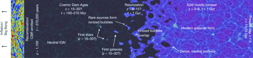
Figure 1: A graphical overview of the main phases of neutral and ionized hydrogen in the Universe. From Robertson et al. (2010).

2.2 Current constraints on the Cosmic Dawn and Epoch of Reionization

Even though the history of neutral hydrogen is crucial to our understanding of the high-redshift Universe, very little is known about it. There is only a handful of observations that currently constrains physical models of the evolution of neutral hydrogen:

• the Gunn-Peterson trough at/near the end of reionization from which (a limit on) the HI optical depth can be inferred (e.g. Becker et al., 2001; Fan et al., 2002, 2006),

• the discovery of Gamma-Ray Bursts (GRB) during and after reionization (e.g. Ruiz-Velasco et al., 2007; Sparre et al., 2014) from which the high-mass star-formation rate (SFR) can be inferred,

• the metal abundances and old stellar populations (e.g. Simcoe et al., 2012) possibly in Damped Lyman Absorbers (DLAs),

• the evolution of the IGM temperature after reionization from which a nominal reionization redshift can be inferred, if the IGM cooled adiabatically and did not re-heat (e.g. Theuns et al., 2002; Bolton et al., 2010),

• the polarization of the CMB due to ionized gas (basically electrons) integrated along the line-of-sight to the present day from which a median reionization redshift and duration can be inferred (see e.g. Robertson et al., 2015),

• the integrated IR and X-ray backgrounds setting limits on the emission from the first (Population III & II) stars, X-ray sources and quasars (e.g. Zemcov et al., 2014; Fernandez & Zaroubi, 2013; Helgason et al., 2014)

• the observations of the first galaxies through drop-out techniques, currently out to $z\sim 12$ already (e.g. Ellis et al., 2013), or Lyman-$\alpha$ emission (e.g. Matthee et al., 2014), providing limits on ionizing (stellar) sources, and the HI content in the IGM from Lyman-$\alpha$ emitters.

Although theoretical models are highly degenerate especially at increasingly larger redshifts, it does appear from these observations that reionization is roughly half-way at $z\sim 10$, followed by a rapid increase in the SFR-density below this redshift (e.g. Lorenzoni et al., 2011; Bouwens et al., 2012; Ellis et al., 2013). Around $z\sim 5-7$ potentially 10% of hydrogen could still be in neutral patches (e.g. Mesinger, 2010), although most of it was (re)ionized by then, making most of the the universe transparent to uv-radiation all the way to the present day. Beyond $z\sim 10$ even less is known and most of what we think was happening is actually based on theory (e.g. Pop-III stars) and simulations that are constrained by physical models extrapolated from lower redshifts (e.g. X-ray heating via XRBs; Fialkov et al., 2014b). It it therefore crucial that new observational avenues are explored to open up these early phases in the Universe for observational studies. The redshifted 21-cm emission of neutral hydrogen provides just such a possibility. Neutral hydrogen is all-pervasive until its (re)ionization completes and it complements (i.e. anti-correlates) with sources of ionization, with the CMB and with the IR/X-ray background (although see Fialkov et al., 2015). Moreover due to the line-nature of the 21-cm hyperfine transition, redshift (and velocity) information can be gained directly from 21-cm emission by fine-tuning observations to different radio frequencies [i.e. to $1420/(1+z)$ MHz]. Hence tomography of (redshifted) 21-cm emission can be done by covering a wide range of frequencies.

In the case of the SKA, frequencies of 50 MHz (during phase 1) and higher allow HI mapping at redshifts below $z\sim 27$ ($\sim\,120$ Myr after the Big Bang) all the way to the end of reionization $z\sim 5-6$ ($\sim 1$ Gyr after the Big Bang). Especially the highest redshifts are extremely hard to reach with other instruments, even with the James Webb Space Telescope (JWST) in the next decade.

2.3 Current 21-cm detection experiments

There are two general approaches to observe HI emission via the 21-cm line: (i) its spatially-averaged global signal and (ii) its spatial fluctuations, both as function of frequency (i.e. redshift, time, distance). In the former case the average redshifted 21-cm emission at a given redshift is measured over a very large (possibly global) area of the sky such that spatial fluctuations are averaged away, in general via single dipoles or fully-filled antennae (e.g. dish, aperture arrays with near unity filling factor). The global signal can vary between a few mK brightness temperature near the end of reionization and around those redshift where the HI spin temperature and the CMB were almost same, to as much as +30 mK when the spin temperature was well above the CMB temperature, and to as low as $-$100 mK or even less during the Cosmic Dawn when HI was seen in absorption against the CMB and the spin-temperature coupled to the cold neutral gas. Whereas in principle these signals could be detected in a few hours to a few days based purely on thermal noise limits, such a detection turns out to be extremely difficult to the high dynamic range that is needed in band-pass calibration (i.e. $>10^{6}$), in the presence of RFI and the complex spatially-temporal-frequency varying sky that couples to a generally polarized and frequency-dependent receiver beam. Whereas many global experiments are ongoing (e.g. EDGES, CORES, SARAS, LEDA, etc; see Subrahmanyan et al. 2015) none have reached the few to tens of mK level yet required for a solid detection although bandpass stability of $\sim 1$ K has now been reached (Patra et al., 2013, 2015).

An alternative/complementary approach to detect the redshifted 21-cm emission is via an interferometer, which is insensitive to the global signal (which is detectable on the (near)zero spacings only), but can only detect fluctuations in the 21-cm brightness temperature. Although these fluctuations can be considerable, they are far smaller in amplitude than the global signal hence requiring long ($\sim$1000 hrs) of integration time to detect. At lower redshifts during the Epoch of Reionization, however, ionized bubbles could be $-30$ mK in depth and detectable on somewhat longer baselines with arcmin resolution. Apart from the ionized bubbles, brightness temperature fluctuations are sourced by density fluctuations in the time-evolving dark-matter distribution and via the spin-temperature coupling to the neutral gas and/or the CMB, though the Wouthuysen-Field effect and through heating. In addition, fluctuations are sourced by peculiar and bulk-flow velocities that Doppler-shift the 21-cm line, affecting its brightness temperature. Whereas this complex astrophysics make interpretation of the 21-cm signal harder, it also provides a wealth of information on sources and physical process occurring during that period. In combination with the global signal and other observables (e.g. galaxies, CMB polarization, etc) these brightness-temperature fluctuations provide a treasure trove of information. The second advantage of using an interferometer is to reduce the levels of foreground emission from the Milky Way (several Kelvin versus several hundred Kelvin) that could potentially contaminate the feeble 21-cm signal, as well as the fact that interferometers are often easier to calibrate than total-power experiments. At the moment each of these approaches are pursued by multiple teams and valuable in their own right and targeting different parameter spaces, thereby complementing each other. Current HI detection experiments are ongoing with the GMRT (e.g. Paciga et al., 2011), LOFAR (e.g. Yatawatta et al., 2013; van Haarlem et al., 2013), PAPER (e.g. Ali et al., 2015; Pober et al., 2015), MWA (e.g. Dillon et al., 2014) and observations with the LWA (i.e. LEDA) (e.g. Greenhill et al., 2014), as well as with NenuFAR, under construction, are planned.

2.4 Planned high-redshift 21-cm arrays

Despite great strides forward over the last decade, no high-redshift 21-cm detection has yet been successfully claimed, neither of the global HI signal nor of its fluctuations. Even if successful, all current observational programs (except for those targeting the global signal) aim for a statistical detection via power-spectra (and high-order statistics) and only on the very largest angular scales (degrees) could one potentially reach a S/N$\sim$few in a few MHz frequency bin, comparable to the first CMB maps with COBE (Smoot et al., 1992). To overcome the current S/N$\sim$1 barrier substantially more collecting area is required, especially on short baselines corresponding to a few to tens of arc minute scales, by an order of magnitude over the current LOFAR-core collecting area, the latter being the largest low frequency array currently aiming to detect high-$z$ 21-cm emission. Such a collecting area is foreseen in the current baseline design of SKA1 and might evolve in to SKA2 with four times the SKA1 collecting area (see this volume), allowing one to move from upcoming statistical detections to tomographic (i.e. direct imaging) measurements of HI in the next decade. A similar US-lead effort called HERA is also planned extending the current PAPER project in South-Africa, and NenuFAR in France that aims for a nearly fully filled low-frequency (10-80MHz) array of 400-m diameter.

3 Some relevant physics during the CD/EoR eras

Radio-telescopes measure the sky’s intensity distribution (more precisely its Fourier transform), which traditionally is expressed in terms of a brightness temperature $T_{\rm b}$ in the Rayleigh-Jeans regime. It can be shown that the brightness temperature of neutral hydrogen as function of redshift z, seen against the CMB, can be written as (e.g. Madau et al., 1997):

$$\delta T_{\rm b}=27x_{\rm HI}(1+\delta)\sqrt{\frac{1+z}{10}}\left(\frac{T_{\rm s}-T_{\rm CMB}}{T_{\rm s}}\right)\left(\frac{\Omega_{\rm b}}{0.044}\frac{h}{0.7}\right)\sqrt{\frac{\Omega_{m}}{0.27}}$$

$$\times\left(\frac{1-Y_{\rm p}}{1-0.248}\right)\left(1+\frac{1}{H(z)}\frac{dv_{||}}{dr_{||}}\right)^{-1}{\rm~{}~{}~{}mK}.$$ (1)

This equation contains several terms set by cosmology (i.e. the global baryonic density and spatial density fluctuations, $\Omega_{\rm b}$ and $\delta$, respectively; the total mass density and the Hubble constant $\Omega_{\rm m}$ and $H(z)$ or $h$, respectively), by (g)astro-physics (i.e. the spin-temperature $T_{\rm s}$ of HI, the CMB temperature $T_{\rm CMB}$) and by Doppler effects ($dv_{||}/dr_{||}$; e.g. due to peculiar motions and bulk-flows of the gas). Via the brightness temperature and different measures of it, e.g. variance, higher-order statistics, power-spectra, $n$-point correlations, tomographic cubes (i.e. images), HI-absorption spectra, cross-correlation, etc., one can address questions about the physics and sources responsible for processes during the CD/EoR such as heating (changing $T_{\rm gas}$), Lyman-$\alpha$ emission and the Wouthuysen-Field effect (changing $T_{\rm s}$ via $T_{\rm gas}$; Wouthuysen (1952); Field (1958, 1959)), reionization (changing $x_{\rm HI}$) and the growth of density fluctuations and peculiar velocities (changing $\delta$ and $dv_{||}/dr_{||}$).

3.1 Phases of 21-cm emission and absorption

Largely due to the expansion of the universe and within it the gravitational collapse of matter, the universe at some point becomes non-linear in its (evolving) density structures producing the first stars, stellar remnants, black holes, and galaxies. These objects in turn will impact the IGM/HI surrounding them, leading to a host of observational effects that can be used to assess their properties. Below we shortly summarize the main phases of HI after recombination ($z\sim 1100$) and before complete reionization ($z\sim 5-6$). We again refer to Barkana & Loeb (2001); Furlanetto & Briggs (2004); Lewis & Challinor (2007); Pritchard & Loeb (2008); Morales & Wyithe (2010); Loeb & Furlanetto (2013); Fialkov et al. (2014a) for many more details.

• Age of Ignorance (z$\sim$1100-200): Just after recombination the spin-temperature of neutral hydrogen tightly coupled to the CMB temperature, indirectly via the gas temperature (via Compton scattering), making the 21-cm line invisible against the CMB temperature. At the moment no known observational technique is able to probe this era, even if it were possible at these high redshifts. Observing these high redshift using the 21-cm line would first of all have to be carried out in space to avoid the ionospheric plasma frequency, but most likely would be limited by self-absorption in the MW (Novaco & Brown, 1978). In case of dark-matter annihilation (see e.g. Valdés et al., 2013) or other heating sources (Lyman-$\alpha$ photons from recombination; (see Fialkov & Loeb, 2013)) could one conceivably have the spin-temperature decouple from the CMB temperature. However, it is likely that this period in the history of the Universe will remain out of reach till far in the future, and remain a true Age of Ignorance.

• Dark Ages (z$\sim$200-30): About five million years after recombination the spin-temperature of hydrogen coupled – via trace electrons – to the colder-than-the-CMB gas-temperature. Neutral hydrogen became visible in absorption again the CMB during that era. At the end of the Dark Ages the density of trace electrons, however, dropped sufficiently (through expansion of the Universe) to make the coupling of the spin and gas temperature inefficient. The spin temperature started to follow the CMB temperature again and $T_{\rm b}$ approached zero from below. However, this phase just preceded the formation of the first radiating sources and probably only lasted briefly or might not even have been fully reached (i.e. $T_{\rm b}\sim 0$ mK). Processes that can be studied through measurements of $T_{\rm b}$ during the Dark Ages are the dark-matter power-spectrum evolution and its annihilation physics, baryonic bulk-flows (Tseliakhovich & Hirata, 2010) and the physics of gravity and general relativity. The physics during this era can largely be understood through linear theory (Lewis & Challinor, 2007), or linear corrections thereof (e.g. Ali-Haïmoud et al., 2014) and deviations of observation from CDM predictions will immediately indicate new physics. Studying HI deep in to the Dark Ages however will remain out of reach in the near future and requires space-based radio telescopes because 21-cm emission will have been redshifted to near or below the ionospheric plasma frequency.

• Cosmic Dawn (z$\sim$30-15): The Cosmic Dawn is typically defined as the time when the first stars (or other radiating sources) were formed. Lyman-$\alpha$ emission from these sources efficiently coupled the spin temperature to that of the cold gas (via the Wouthuysen-Field effect), again leading to neutral hydrogen seen in absorption. At the same time, however, the gas itself was heated supposedly via X-ray heating or, possibly, via the hot ISM and Lyman-$\alpha$ photons (Pacucci et al. 2014). This gas-heating and the parallel process of coupling the spin and gas temperature led to a rapid rise in the brightness temperature of neutral hydrogen until it is finally seen in emission around $z\sim 15$. One should note that many of these processes are still ill-understood and all these effects (heating, coupling, etc) could shift around in redshift substantially, especially between the Cosmic Dawn and the Epoch of Reionization. Hence when these processes exactly occurred is not known and redshifts indicated here are merely indicative numbers currently expected from nominal models. Processes that can be studied during the CD are the formation of the first (pop-III) stars, the first BHs, X-ray heating sources, W-F coupling, bulk-flows, etc.

• Epoch of Reionization (z$\sim$15-6): While heating together with the W-F effect change the spin-temperature of the neutral hydrogen, the same radiation field (i.e. uv-radiation) starts to ionize hydrogen leading to the percolation of bubbles around the first mini-haloes containing (Pop-III) stars and possible intermediate mass black holes, i.e. mini-quasars. As time progresses and the universe becomes increasingly more non-linear (on small scales), more stars and quasars are formed. Although recombination can have some impact (see e.g. Sobacchi & Mesinger, 2014), it can not stop or balance ionization in an expanding universe and by $z\sim 6$ the entire universe, apart from pockets of neutral hydrogen (mostly in galaxies), will be ionized once more. Processes that can be studied during the Epoch of Reionization are the physics of the ionizing sources, such as pop-III and II stars, mini-quasars, feedback to the IGM and the transition to the currently visible universe.

• Post-Reionization (z¡6): Whereas most neutral hydrogen will have been ionized, pockets of neutral hydrogen might remain even at lower redshifts and in galaxies (e.g. Mesinger, 2010), which could be studied though intensity mapping and via cross-correlations with other e.g. IR surveys (see this volume).

3.2 Sources of heating, radiation, feedback and ionization

Whereas the above situation delineates general eras during which certain physical processes (e.g. Lyman-$\alpha$ emission, heating, ionization, etc) might dominate, the understanding of these processes is far from certain and depends strongly on the types of sources responsible for uv- and X-ray emission. Via their imprint on the brightness temperature of neutral hydrogen one can gain insight in to these first radiating sources, which is one of the main reasons to study high-$z$ 21-cm emission. Below a range of sources is listed that are currently thought to play a role. We refer to the accompanying chapter in this volume for more details.

• Population-III and -II Stars

  The first stars presumably formed just after the Dark Ages from relatively pristine gas (primordial abundances), and will soon be detectable by upcoming missions, such as JWST, through their supernova explosions (de Souza et al. 2013, 2014). These first stars (Pop-III) are thought to have been of high mass, although recent work suggests they fragmented possible into stars of several tens of solar masses (e.g. Stacy & Bromm, 2013). It is the uv-radiation of these stars that is thought to couple the hydrogen spin temperature to that of the cold gas. Emission from resulting X-ray binaries (XRB) could subsequently lead to X-ray heating. In addition, the first and second generation (Pop-II) stars are thought to be responsible for the ultimate (re)ionization of nearly all neutral hydrogen during the Epoch of Reionization. What the relative roles of Pop-III and Pop-II stars exactly are in these processes, i.e. W-F coupling, heating and ionization, is currently ill-understood and the processes involved in the formation of Pop-III stars and whether they form the seeds for SMBHs is also not clear. At lower redshifts where the first galaxies can be observed, however, it is clear that stars responsible for reionization must be in mini-haloes and in galaxies $\sim$500 times fainter ($\sim$7 mag.) than current observational limits (e.g. Davé et al., 2006). Hence enormous extrapolations are needed to make any inference from current observations, let alone to redshifts even higher. Redshifted 21-cm emission observations clearly are important in setting limits on star formation and the types of stars (or AGN) that partake in the early phases of the CD/EoR eras.

• Mini-Quasars and AGN

  A second source of ionization and heating can be intermediate-mass black holes (IMBHs) and resulting mini-quasars due to accretion discs or Bondi accretion (e.g. Dijkstra, 2006). Whereas it is thought that mini-quasars are not the dominant source of ionizing photons, they can still play a secondary role and possibly be a source of harder X-ray photons that can more uniformly heat the IGM well above the CMB temperature. These IMBHs are also thought to be the seed-BHs of present-day SMBHs and AGN, although the process of accretion appears to be super-Eddington to have them grow from 100 solar masses (expected from massive Pop-III stars) to $10^{9}$ solar masses in the AGN seen already at $z\sim 7$ (Mortlock et al., 2011).

• X-ray Binaries

  Great uncertainty also remains whether X-ray binaries are sources of heating at high redshifts and whether heating takes place on global scales. If heating is inefficient some IGM patches could remain very cold and below the CMB temperature causing the redshifted 21-cm brightness temperature to remain in absorption substantially impacting the level of strength of the total-intensity and fluctuation signals from neutral hydrogen. This could lead to considerable effects even at very low redshifts during the Epoch of Reionization (e.g. Pritchard & Loeb, 2008).

• Dark-Matter Annihilation

  Literately a ”Dark Horse” is whether dark matter could be a source of ionization or heating at very high redshifts during the Dark Ages, already influencing the evolution of the IGM well before the Cosmic Dawn (e.g Taoso et al., 2008; Ripamonti et al., 2010).

Having outlined a number of important eras as well as the physics and source responsible for the brightness temperature evolution of neutral hydrogen (both spatially and in time), we now continue to discuss which observables the SKA can obtain and use to constrain these processes and from it learn about the sources responsible. We also shortly mention possible synergies with other (planned) facilities.

4 Observables via the redshifted 21-cm brightness temperature

Redshifted 21-cm emission from neutral hydrogen manifests itself in multiple ways and various methods and techniques can be used to extract information from it. In the following section we discuss a number of such approaches, whereas in the subsequent section a short summary is given of other observables (and facilities) that the 21-cm brightness temperature could be cross-correlated with. We refer to Mellema et al. (2013), as well as to Chang et al. (2015) and Jelic et al. (2015) in this volume, for more details on the synergy between the SKA and other observatories.

4.1 Measures of the brightness temperature field

All of the information one hopes to gain from the physics occurring during the Dark Ages, Cosmic Dawn and Epoch of Reionization from neutral hydrogen is obtained via its redshifted 21-cm brightness temperature. As shown in Section 3, this temperature is set by a combination of many different physical processes which need to be disentangled. As of yet, it is not fully clear whether this can be done completely or not. In addition, it is likely that in the first experiments, also with the SKA1, only limited measurements of the brightness temperature will be made. Below we summarize some of the standard measures of $T_{\rm b}$:

• Total Intensity Redshifted 21-cm emission of neutral hydrogen averaged inside ”shells” of common redshift (or observed frequency) are close to impossible to measure with interferometers since they measure intensity differences (Subrahmanyan et al. 2015). However, as seen in Section 3, the total expected brightness temperature is of order $\sim 27x_{\rm HI}(1+\delta)$ mK at $z\sim 10$ if $T_{\rm s}\gg T_{\rm CMB}$. When averaging over large areas of the sky ($\gg 1$ degree) $\langle\delta\rangle\approx 0$ and assuming no reionization (i.e.  $x_{\rm HI}=1$), one can determine the total intensity of the signal. This is ”most easily” achieved with single receiver/dipole measurements and is discussed in much greater detail in Subrahmanyan et al. (2015). Measuring this signal as function of redshift allows one to learn about different physical processes such as Lyman-$\alpha$ coupling by the first stars, heating by (X-ray) sources, reionization, etc. At this point it is not clear whether the SKA will be capable of measuring this signal since it requires a very accurately calibrated instrument.

• Variance or second moment The second-order effect comes from variations in the brightness temperature due to variations of $\delta$, $x_{\rm HI}$, $T_{\rm s}$ and $v_{||}$. These variations lead to a spatial variance in $T_{\rm b}$ as function of observed frequency or redshift (see Mellema et al. 2015 and Wyithe et al. 2015) which can be measured in interferometric images, assuming that systematics and thermal noise are under control and/or known (although thermal noise can be removed via cross-variance techniques over small time-frequency steps). By measuring the variance one can again learn how HI evolved over cosmic time, in particular when reionization peaked (the contrast between HI and bubbles is very large and leads to a large variance). However, the shape of PDF($T_{\rm b}$) also teaches us about its moment (skewness and/or kurtosis) again revealing information about reionization (e.g. Harker et al., 2009). In particular the skewness of the PDF might be a tell-tale signature of reionization that would be hard to mimic by systematic effects (which often are strongly correlated between frequency and scale smoothly with frequency as well).

• (Anisotropic-)Power-spectra One step further would be the analysis of $T_{\rm b}$ in the Fourier domain in terms of the variance as function of spatial (or angular) scales, i.e. the power-spectrum. The power-spectrum depends on the spatially varying parameters in Equation 1, being $x_{\rm HI}$, $\delta$, $T_{\rm s}$ and $v_{||}$. All other parameters can be assumed constant and only enter via the general FRW metric. The power-spectrum is directly related to the underlying local physical processes and sources of reionization (governing $x_{\rm HI}$), heating (governing $T_{\rm s}$), as well as to the evolution of the density field (governing $\delta$ and $v_{||}$). To first order one can Taylor expand equation 1 in these parameters, Fourier transform the result, from which the power-spectrum can be formed. Since the parameters are not independent (e.g. an over-density can also lead to extra heating and ionization), the resulting 21-cm power-spectrum becomes a rather complex function of these parameters and their cross-correlations, and can become anisotropic. These can either be determined via simplified schemes or via direct numerical simulations (which also contain simplified sub-grid physics). Disentangling all effects from the power-spectrum as function of redshift is nontrivial and remains an ongoing and active research field. To first order, the power-spectrum is isotropic and can be spherically averaged (where the frequency direction over some limited bandwidth is a proxy for comoving distance, hence inverse wavenumber), although in the case of SKA (possibly even before) the sensitivity if sufficient to measure anisotropy in the power-spectrum which can be an exciting measure of underlying physics (e.g. Fialkov et al., 2015). Hence it is often better to express the power-spectrum in two dimensions, separating the wave vector in a component perpendicular to the line of sight and a component parallel to it, in particular to study peculiar velocities, the light-cone effect, as well as potentially identify still-remaining systematic errors in the data-processing.

• Higher-order statistics/n-point correlations: Already touched up on above, the brightness temperature field after the Dark Ages will start to deviate from a Gaussian random field. This means that the power-spectrum or two-point correlation function will become an increasingly more incomplete description. The brightness temperature difference between two points will deviate from a Gaussian distribution, and the three and high-point statistics will become non-zero (Pillepich et al., 2007; Cooray et al., 2008). Studying these statistics can therefore provide additional information about physical processes, even if direct imaging might still be infeasible.

• Tomography/Images: The ultimate goal of any HI observation is make direct images and determine the brightness temperature with high significance for each spatial-frequency cell (see Mellema et al. 2015 and Wyithe et al. 2015 this volume). This clearly contains the maximum amount of information obtainable from the data-set, but interpretation is not always straightforward and the analysis of images has been a sorely neglected topic in the literature. In fact, even from direct numerical simulations, results are often presented in limited statistical measures such as the power-spectrum. Developing new ideas on how to analyze brightness temperature images is therefore crucial before the SKA comes online since it will be the first instrument capable of imaging/tomography on scales of several arc minutes to degrees. Only in exceptional cases might one expect to do this pre-SKA.

• Bubbles and HI topology: Whereas initially imaging of HI brightness temperature fluctuations at the level of several mK might not be feasible (e.g. in roll-out, etc), the stark contrast of 20-30mK and size (ten(s) of Mpc) of ionized bubbles will probably allow them to be seen relatively easy on during the roll-out and later phases of SKA1 imaging. Their distribution as function of size, shape, etc. will likely reveal swiftly how reionization proceeded (i.e. inside-out, or otherwise). It might also reveal the nature of the sources causing reionization, in particular if (mini-)quasar play a role. Although some of this information is encoded in the power-spectra (which forms from a combination of the non-ionized HI field times a mask where HI has disappeared) their precise sizes, shapes, etc. will provide a far richer source of information. In addition it might be possible to study the local velocity field structure around bubbles which might reveal additional information that the power-spectra do not.

• 21-cm absorption: Whereas all the above measures of neutral hydrogen are based on its brightness temperature contrast with the CMB, there could be radio sources (mJy or brighter) present at sufficiently high redshift that the 21-cm line could be see in absorption against such source (e.g. Carilli et al. (2002) and Ciardi et al. 2015). A mJy source (e.g. AGN or GRB) of a few arcmin resolution at say 150MHz would already be sufficient to measure the HI forest and from it (equivalent to the Lyman-$\alpha$ forest) measure the line-of-sight power-spectrum of neutral hydrogen. Although success depends on the (still unknown) presence of radio sources at redshifts well beyond the end of reionization, it would provide a unique opportunity to measure $P_{21}(k)$ on $k$-modes far larger (i.e. scales far smaller) than accessible via imaging/tomography or power-spectra as discussed above. As such SKA1 and 2 could provide the first measures of mini-haloes during the Epoch of Reionization something that even JWST will find difficult to do.

4.2 Synergy with other surveys/Cross-correlations

Whereas SKA will characterize the brightness temperature in detail via either power-spectra, direct imaging or 21-cm absorption possible to redshifts of $z\sim 27$ during the Cosmic Dawn, and will be unique at this, complementary observations can further enhance the capability to extract information from this rich data-set. Among these are: (1) the Planck (or future) CMB maps, (2) the Far-Infrared background or emitters, (3) surveys of high-$z$ Lyman-$\alpha$ emitters, (4) high-$z$ Lyman-break Galaxies/Dropouts, (5) high-$z$ SNae/GRB transients, (6) CO/CII emitters and (7) DLAs. We refer to Chang et al. (2015) and Vibor et al. (2015) in this volume for details.

5 Survey Design

In this section we outline a potential observational survey with SKA1 (and 2) to characterize the redshifted 21-cm brightness temperature of HI between $z=27$ ($\nu$=50MHz) and z$\sim$6 (end the EoR), via its two main observable: power-spectra and tomography. We assume throughout that calibration and foreground subtraction is done to a level accurate enough that it does not affect the resulting residual data-cubes (containing both the 21-cm signal as well as noise). For more details on the latter we refer to Mellema et al. (2013). Hence thermal noise and sample variance (in the case of power-spectra) are assumed to dominate the error budget in the power-spectra and thermal noise dominates the error-budget in the images.

5.1 Scaling Relations for power-spectrum sensitivity

To understand the choices of survey specifications we need some guidance. This is most easily understood by assuming a uniform $uv$-coverage in an interferometric experiment. As shown in Mellema et al. (2013) and based on McQuinn et al. (2006), the power-spectrum error due to thermal noise is then given by:

$$\Delta^{2}_{\rm Noise}=\left(\frac{2}{\pi}\right)k^{3/2}\left[D_{\rm c}^{2}\Delta D_{\rm c}\Omega_{\rm FoV}/N_{\rm b}\right]^{1/2}\left(\frac{T_{\rm sys}}{\sqrt{B\,t_{\rm int}}}\right)^{2}\left(\frac{A_{\rm core}A_{\rm eff}}{A_{\rm coll}^{2}}\right)$$ (2)

The total error is obtained by adding the sample variance to this, which depends on the power-spectrum of the signal itself and the number of independent samples per volume. Whereas this equation gives a reasonable idea of the level of thermal noise variance on 21-cm power-spectra, it can be tilted as function of $k=2\pi/L$, depending on the $uv$-density as function of baseline length. In this equation, the co-moving distance to the survey redshift is $D_{\rm c}$, the depth of the survey for a bandwidth $B$ is $\Delta D_{\rm c}$ and the field-of-view of the survey is $\Omega_{\rm FoV}$. In case of multi-beaming, the number of independent beams is $N_{\rm b}$. A system temperature of $T_{\rm sys}$ is assumed and an integration time $t_{\rm int}$. Each station/antenna is assumed to have an effective collecting area $A_{\rm eff}$, that corresponds to the field-of-view as $\Omega_{\rm FoV}\equiv\lambda^{2}/A_{\rm eff}$, where $\lambda$ is the wavelength at the center of the frequency band. The antennae are distributed over a core area $A_{\rm core}$ in such a way that the $uv$-density is uniform and the total collecting area (the sum of all effective collecting areas of each receiver) is assumed to be $A_{\rm coll}$. The equation has been shown to be correct via numerical integration, using the method outlined in McQuinn et al. (2006). Regardless the assumption of a uniform $uv$-density (which affect the exponent in $k^{3/2}$ and the normalization), the scaling with the layout of the array follows

$$\Delta^{2}_{\rm Noise}\propto\left(\frac{A_{\rm core}\sqrt{A_{\rm eff}}}{A_{\rm coll}^{2}}\right)\propto\left(\frac{A_{\rm core}}{N_{\rm stat}^{2}A_{\rm eff}^{3/2}}\right)\propto\left(\frac{A_{\rm core}}{\sqrt{N_{\rm stat}}A_{\rm coll}^{3/2}}\right)$$ (3)

where we assume $A_{\rm coll}=N_{\rm stat}A_{\rm eff}$ with $N_{\rm stat}$ stations/receivers. Given the above equation and scaling relations, a number of conclusions can be drawn for the power-spectrum sensitivity at a given $k$-mode scale: (i) sensitivity scales most rapidly with collecting area, (ii) increasing field-of-view helps, but only with the square root of the field of view, and (iii) more compact arrays (still covering the $k$-modes of interest) are more sensitive. All current arrays (i.e. MWA, LOFAR and PAPER) follow strategies that optimize (or maximize within budgetary limits) these three parameters. SKA1 and 2 will both increase $A_{\rm coll}$ by 1-2 order of magnitude over all current arrays and minimize $A_{\rm core}$ by maximizing the filling factor and placing much of the collecting area in a rather small core area. Finally, based largely on computational limitations, the field of view of SKA is at least of order five degrees at 100 MHz, but during later phases (e.g. SKA2) could be increased through either multi-beaming or through reducing the beam-formed number of receivers. Although in considering optimizing an array for CD/EoR science, one should not forget that the system also needs to be calibrated for instrumental and ionospheric errors, and foregrounds (compact and extended, in all Stokes parameters) need to be removed, which might require the use of long baselines. Any array, also SKA1 and later 2, therefore preferably would consist of a compact core with ”arms” extending to many tens of kilometer.

5.2 Scaling relations for tomography/imaging

Similar to the power-spectrum sensitivity, one can also obtain a scaling relation for imaging or tomography. One readily finds that the thermal noise inside a resolution element corresponding to a scale $k_{\perp}$ scales as:

$$\Delta T = \left(\frac{k_{\perp}}{2\pi}\right)\left[D_{\rm c}^{2}\times\Omega_{\rm FoV}\right]^{1/2}\left(\frac{T_{\rm sys}}{\sqrt{B\,t_{\rm int}}}\right)\sqrt{\left(\frac{A_{\rm core}A_{\rm eff}}{A_{\rm coll}^{2}}\right)}$$ (4)

$$= \left(\frac{k_{\perp}}{2\pi}\right)\left[D_{\rm c}^{2}\times\Omega_{\rm core}\right]^{1/2}\left(\frac{T_{\rm sys}}{\sqrt{B\,t_{\rm int}}}\right)f_{\rm fill}^{-1},$$

assuming a sinc-function as model for the sky-components (i.e. a top-hat in uv-space). In this case $A_{\rm eff}$ drops out of the equation, although we leave it in to retain a similar form to the equation for the power-spectrum. We also see that on larger angular scales (i.e. smaller $k_{\perp}$), the noise decreases and that a more compact array helps to reduce the thermal noise per resolution element, by increasing the number density of visibilities per $uv$-cell. The latter form of the equation expresses this through the filling factor ($f_{\rm fill}$) of the core area in terms of collecting area and the field-of-view in a resolution element of the core. Filtering longer baselines (or smoothing of the image) to a resolution corresponding to $k_{\perp}$ averages down the noise and lowers the brightness temperature error, hence $k_{\perp}$ does not necessarily correspond to the largest baseline afforded by the core area. The latter simply sets the $uv$-density. For example for the inner part of SKA1 the core of 400m diameter has $f_{\rm fill}\sim 1$ and on scales $k_{\perp}=0.1$ cMpc^-1 ($\sim 20^{\prime}$) one expect an error of $\sim 0.2$ mK per MHz in 1000 hrs of integration time at 150MHz, assuming $T_{\rm sys}=400$ K, which is below the expected brightness temperature fluctuations on that scale. However, with increasing resolution the filling factor of the core decreases and $k_{\perp}$ increases, both leading to a rapidly increasing brightness temperature error ultimately limiting the angular scale where imaging can still be done. For SKA1 and 2 this limits occurs on an angular scale of a few to about ten arc minutes in a reasonable ($\sim$1000 hr) integration time.

5.3 Current SKA1-LOW Baseline Design and its Relevant Design Specifications

In the following we assume the current SKA1 baselines design (BLD), based on the station layout provided in Braun (2014). Although the latter is not necessarily the ultimate layout, it represents a ”close-enough” description of the array that no major differences are expected in the resulting sensitivity calculations, except if the array is (i) substantially thinned out (i.e. reducing the total collecting area), (ii) dramatic changes in antenna layout are introduced (i.e. changing the filling factor) or (iii) substantially reducing the instantaneous field of view (i.e. through beam forming larger numbers of receiver elements). We refer to other chapters in this volume for a full description of the current BLD. Using these antenna positions (or radial distribution) we calculate full 12-hr $uv$-tracks in the direction of the South Galactic pole and average the $uv$-density within radial bins. Similar densities are obtained for tracks at lower elevations. We assume a nominal 35m beam-formed ”station” as well, which leads to a frequency-dependent field-of-view, being around 5 degrees FWHM at 100 MHz.

The fiducial layout that we assume in this review is listed below. We emphasize that this is not necessarily the most optimal observing strategy, although in some cases (e.g. freq. coverage) full use of the capabilities of SKA1 and 2 are made. As we will discuss below, multi-beaming can dramatically improve the return of a single CD/EoR survey. Also integration times can be increased. Finally we assume for the nominal survey that phase-tracking of a single field is done, rather than drift-scans although we come back to that in this Section and Section 6.3.

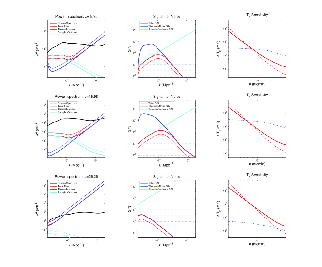
Figure 2: Deep Survey: Shown are the expected brightness temperature power-spectra from Mesinger et al. (2014) and the expected thermal-noise and cosmic-variance errors (following McQuinn et al., 2006) for the fiducial deep-survey parameters outlined in the text for SKA1-LOW. The thick/thin curves are for 5 versus 1 beam. The middle-column panels (red curves) indicate the expected total S/N ratio in such a deep survey, reaching a peak S/N$\sim 70$, in good agreement with the results in Mesinger et al. (2014). The right column panels show the brightness temperature sensitivity as function of resolution, where the $k$-scale is transformed directly to angular scale at the corresponding redshift. The latter does not depend on the number of beams. The dashed line is for a BW that matches the angular scale rather than being fixed to 10MHz. The blue dot-dashed line is the expected variance on that scale by integrating over the power-spectrum.

1. Antenna layout: We assume for SKA1 the layout as (generically) specified the BLD, assuming that for SKA2 the collecting area is increased by a factor of four. The latter is implemented here via a scaling of all baselines by a factor of two and quadrupling the number of stations at each SKA1 station position. This ensures that the filling factor in the core remains of order unity and decreases in a scale-invariant manner to SKA1. Other choices are possible and will be investigated in the future.

2. Frequency range: Based on the current baseline design of SKA1, we assume a full instantaneous frequency coverage of 50–350 MHz (i.e. $z$=27-3). This range is thought to encompass the full Cosmic Dawn and Epoch of Reionization (see Mellema et al., 2013). We assume that during SKA1 the bandwidth can at least be split in two beams of 150-MHz, increasing the survey speed by a factor two. We note again that more beams can reduce on-sky time significantly. In the future one might consider extending SKA1 to lower frequencies (below 50 MHz) during the upgrade/extension to SKA2, although this will not be considered in this chapter.

3. Survey FoV: The field of view of a single primary beam is assumed to be FWHM$\approx 5^{\circ}$ at 100 MHz. At a redshift of $z\sim 10$, the comoving distance is $\sim 9700$ cMpc, hence the comoving scales covered by the primary beam extend up to $\sim$1 cGpc, about ten times larger than the scale where the dark-matter power-spectrum peaks ($\sim 100$ cMpc). For a bandwidth of 10 MHz (see below), the volume depth is $\sim 170$ cMpc. This means that sample variance on scales of a few hundred cMpc is $\sim 10\%$ and less on smaller scales. On larger scales, sample variance rapidly increases and only a larger survey volume (i.e. increased field-of-view via multi-beaming or drift-scanning) can further reduce this source of variance. One might consider increasing the FoV by beam forming a smaller number of log-periodic elements. We discuss the effect of multi-beaming/increased FoV below.

4. Integration times: In this review, we assume an integration time of 10, 100 and 1000 hrs, for the different levels in a three-tiered survey with decreasing survey area, respectively. The reason for this choice is that SKA1 can reach levels of $\sim$1 mK in 1000-hrs integration time (per 1-MHz bandwidth) over a wide range of angular scales. However, this integration should only be thought of as a reference, since the level of brightness temperature can vary between models. This integration time is also often used in the literature as a reference, making comparison between models easier. The overall on-sky time of the assumed (three-tiered) survey, however, will be larger (see Section 6).

5. Frequency Bandwidth/Redshift Binning: We assume a bandwidth of 10 MHz, per redshift bin (not in total!), to maximize sensitivity but minimize light-cone effects, i.e. the impact of the evolution of the hydrogen brightness temperature with redshift mixed with the assumption that redshift can be regarded as a third spatial dimension of the data volume. The assumed bandwidth is a reasonable compromise. We note that bandwidth enters both in the survey depth (via $\Delta D_{\rm c}$) and in the sensitivity per visibility.

6. Multi-Beaming: We assume a single primary beam ($N_{\rm b}=1$) for a 35m station in SKA1 for the full bandwidth (BW), possible two when split in to two 150-MHz bands, increasing for SKA2 potentially to covering the full log-period dipole beam ($N_{\rm b}\gg 1$). The latter would require an increase in correlator capacity beyond the currently envisioned SKA1 correlator. Below we will show the impact of multi-beaming, in particular in dramatically reducing sample variance on large angular scales.

7. System Temperature: We assume $T_{\rm sys}=100+400\times(\nu/150{\,\rm MHz})^{-2.55}$ K. Although this can change from field to field and can increase/decrease towards/away from the Galactic plane, we assume it to hold to reasonable order and is typical for assumptions in the literature.

8. Inner-Cut uv-plane: Finally we assume a 30-$\lambda$ inner cut to the $uv$-plane (i.e. the sky-projected baselines in units of wavelength) to reduce the impact for foreground leakage in to the power-spectrum. This starts limiting scales $k<0.02$ cMpc^-1 in the power-spectrum (See Fig.2) corresponding to scales of about 2 degrees or $\sim 300$ cMpc at 150MHz. Since these scales already well exceed the peak of the DM and brightness temperature power spectra, they provide some information about cosmology, but far less information of the physics of CD/EoR. This cut is not needed if bright and large scale foregrounds can be controlled.

Whereas these assumptions, based on the BLD of SKA1 and 2 should not be regarded as definitive, they are a guide to typical observations specification, also currently used e.g. by MWA, LOFAR and PAPER, and thus serve as a reference.

6 A Three-tiered Cosmic Dawn and Epoch of Reionization Survey

Having specified our assumed nominal observational settings, in this section, we introduce an outline for a three-tiered survey of redshifted 21-cm emission during the CD/EoR that can address the wide range of physics questions posed in Section 3.

6.1 Main Observation Targets:

It should be stressed that observations of HI emission from the CD/EoR have thus far not been made (although upper limits are currently being set) and any present-day expectations are based on relatively sparse observations in different wavelength regimes or through very different observables(see Section 2.2). Any CD/EoR-HI observational strategy should therefore cover as much of parameter space as possible (e.g. redshift, angular and frequency scales, field of view, etc), providing for surprises that the Universe might put up on us, obviously bounded by any reasonable estimate of what is possible. Overall there are three general approaches to detecting and characterizing neutral hydrogen:

• via direct imaging (i.e. tomography) of neutral hydrogen down to the 1$\sigma\approx 1$ mK brightness temperature level on $>$5-arcmin scales at $z\approx 6$, rising to degree scales at $z$=28.

• via statistical (including power-spectrum) methods to variance levels 1$\sigma\approx 0.01-1$ mK² over the redshift regime $z$=6-28, respectively, at k$<$0.1 Mpc^-1 and to k$<$1 Mpc^-1 at $z<15$.

• via 21-cm absorption line observations against high-z radio sources, if present, with 1-5 kHz spectral resolution (2-10 km/s at z=10) with S/N¿5 on 1 mJy.

• Although SKA2 can attain SKA1’s limits 4$\times$ faster or, in the same integration time go 16$\times$ deeper (for power-spectra), new discoveries with SKA1 are expected to guide SKA2 observations, leading to new observational targets. SKA2 can also image smaller ionized bubbles and sub-mK brightness-temperature fluctuations during the Cosmic Dawn, unfeasible with SKA1. An extension of the frequency range from SKA1 to SKA2 could also enable one to probe the late Dark Ages at $z\sim$30-40.

The general target can be reached in a set of surveys and target fields in three tiers (depth versus area), which we will discuss in the following three sub-sections.

6.2 Deep Survey

The direct science goals of a Deep CD/EoR survey are to detect and characterize ionized structures and HI brightness temperature fluctuations on 5–300 arcmin scales (varying) over the EoR/CD redshift range $z=6-28$ to 1-mK brightness temperature level and from it derive the state, thermal history and chemistry of the IGM, study the first stars, black holes and galaxies and constrain cosmology, the physics of dark matter and gravity. To reach this goal, deep 1000hr integrations are considered on 5 separate 20-square degree windows covering a total of 100 square-degree on-sky area, using the 50-200MHz frequency range with 0.1 MHz spectral resolution (for science), using the full SKA1-LOW array, using multi-beaming with $N_{\rm b}=2$ lowering the on-sky time from 5000 to 2500 hrs. This will not be feasible with any current (or funded) array with S/N$>$1 and is unique to SKA1-LOW. This survey lowers the (expected) thermal noise $\sim 10\times$ over LOFAR and allows direct imaging with S/N$\gg$1. The Cosmic Dawn remains inaccessible to current/funded instruments, until this deep survey with SKA1-LOW. The sensitivities for power-spectra and imaging are shown in Fig. reffig:powerspectra1.

6.3 Medium+Shallow Survey

The direct science goals of a Medium+Shallow CD/EoR survey are to detect and characterize the 21-cm power-spectrum with a peak S/N$\sim$70 measured over $k=0.02-1.00$ Mpc^-1 over the CD/EoR redshift range $z\sim 6-28$ and from it derive the state, thermal history and chemistry of the IGM, study the first stars, black holes and galaxies and constrain cosmology, the physics of dark matter and gravity. A medium-deep pointed survey of 50 times 100-hr integrations would cover 1,000 square degrees, and a preceding shallow pointed/drift-scan survey of 500 times 10-hr integrations would cover 10,000 square degrees, using the 50-200 MHz frequency range with 0.1 MHz spectral resolution (for science) and using the full SKA1-LOW array. Both survey can be carried out in 2500 hours each, assuming two beams of 150 MHz. Again multi-beaming could reduce the on-sky time substantially. A gain in power-spectrum sensitivity would be 1-2 orders of magnitude over current arrays (i.e. MWA, PAPER, LOFAR) in the sample-variance limited S/N regime ($k<0.2$ Mpc^-1), but scales $k=0.2-1$ Mpc^-1 are likely to remain inaccessible until SKA1-LOW is build, because of severe thermal-noise limitations. Again the Cosmic Dawn remains inaccessible to current/funded instruments, until SKA1-LOW is realized. The sensitivities for power-spectra and imaging are shown in Fig.3.

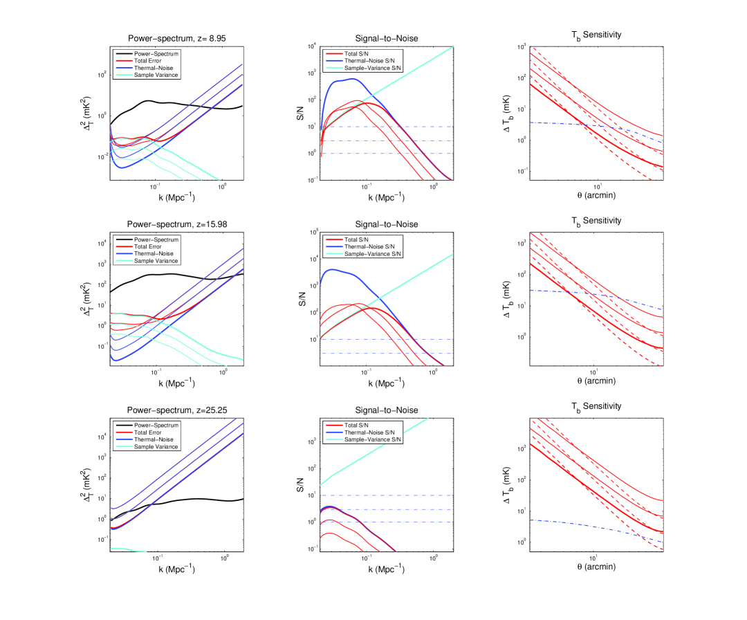
Figure 3: Deep-Medium-Shallow Surveys: Shown are the expected brightness temperature power-spectra from Mesinger et al. (2014) and the expected thermal-noise and cosmic-variance errors (following McQuinn et al. 2006) for the fiducial survey parameters outlined in Section 6 for SKA1. The middle panels (thick red curve) indicate the expected total S/N ratio in such a survey, reaching a peak S/N$\sim 70$, in good agreement with the results in Mesinger et al. (2014). From top to bottom, the red curves for the deep, medium and shallow surveys are shown, clearly showing an increased gain in sensitivity at the larger $k$ modes in the deep survey due to low thermal noise, and an increased gain in sensitivity at the smaller $k$ modes in the medium+shallows surveys due to lower sample variance, leading to a relatively flat S/N curve over one dex in $k$ space. For completeness, the right column show the brightness temperature sensitivity as function of resolution, where $k$-scale is transformed directly to angular scale at the corresponding redshift. From bottom to top are the deep, medium and shallow surveys. The dashed line is for a BW that matches the angular scale rather than being fixed to 10MHz. The blue dot-dashed line is the expected variance on that scale by integrating over the power-spectrum.

6.4 Absorption at 21-cm

The science goal is to obtain 21-cm absorption line spectra from (rare) radio sources at $z>6$ to probe very small scales (i.e. $k\sim 1000$ Mpc^-1) or virialized structures (mini-haloes) and from it derive the state, thermal history and chemistry of the IGM, study the first stars, black holes and galaxies and constrain cosmology, the physics of dark matter and gravity. This can be done through deep 1000-hrs integrations on selected sources with a flux of $>1$ mJy (possibly in the Deep Survey fields; see Ciardi et al. 2015) with a spectral resolution of a few km/s (1-5 khz at 150 MHz) over the 50-200 MHz frequency range ($z\sim 6-28$). We note also here, that no observations of this kind have ever been done and are not expected to be feasible before SKA1-LOW is build, because of the same severe thermal noise limitations that currently limit direct imaging.

6.5 Deep to Shallow Surveys: Multi-beaming and/or Drift-Scans

Optimal observing strategies will depend on many variables: ionospheric conditions, minimization of side-lobe leakage of strong sources, field in the zenith, low galactic brightness temperatures and polarization, optimal $uv$-coverage, multi-beaming versus frequency coverage, inclusion of long baseline information, monitoring of the station beams, RFI excision, drift-scans versus tracking, etc. For SKA1-LOW the field of view is typically 5-10 degrees and hence the sky drifts (see Trott, 2014, for details) though a stationary beam (i.e. non-tracking) in about 0.5-1 hr. Deep integrations of 1000+ hrs would therefore require 1000-2000 nights for every single deep field, which is prohibitively long. Tracking the field over $N$ hrs, would allow the same integration time to be accumulated in $N$ times fewer nights. Hence it appears that drift-scans would only be useful for larger scale shallow surveys, where the total integration per field can be small. On the other hand, because SKA1-LOW allows for two beams in the baseline design, one could conceive of a combination of tracking-drift-scan, where the field drifts from one stationary beam to a second stationary beam and only every 0.5-1 hr would one switch the phase center of the trailing beam to a new phase-center. Since these ideas have not been worked out in detail (but see Trott, 2014), the precise observing strategy remains an open question and will depend on a combination of nights available, sensitivity, resolution in the image, calibration errors, etc.

7 Role-out of SKA1 and expansion to SKA2.

A great advantage of radio interferometers is that it can observe even if incomplete in its number of receiver elements and/or stations/dishes. To enable high-impact science even with an incomplete array it is important to think about rollout from an incomplete SKA1 to a fully complete SKA2.

7.1 Role-out from SKA1 to SKA2: 0.5, 1, 2 and 4 times SKA1

In this section we shortly discuss three stages: (i) roll-out of half of SKA1, (ii) SKA1 and (iii) rollout to a full SKA2, being four times the collecting area of SKA1. We only compare these stagesca assuming a scaling in the number of stations (i.e. collecting area) and no other specification (e.g. frequency coverage, multi-beaming, etc.). The ratio of the number of stations is assumed to be $f_{\rm s}$ where $f_{\rm s}=1$ for SKA1. Since neither half of SKA1 nor SKA2 have any specified baseline designs, we have to make an assumption. Based on the scaling relations in Sections 5, a high filling factor is critical to reach surface brightness levels of $\sim$1 mK. The simplest assumption is therefore to take the current SKA1 BLD and scale the number of visibilities (i.e. the voltage/electric-field coherence between two receivers) by $f^{2}_{\rm s}$, but keeping the radial uv-density profile scale-invariant. The above scalings ensure that the filling factor at the center of the array remains the same during rollout which ensure maximum sensitivity on large angular scales. In Fig.4 we show the impact of $f_{\rm s}=0.5,1.0,4.0$ on the power-spectra and brightness temperature sensitivity for tomography. We conclude a few things in comparison to the SKA1 baseline design:

• For $k<0.1$ Mpc^-1 there is no power-spectrum sensitivity loss in a single beam ($\sim 20$ square degrees) because one is sample-variance limited. Above $k>0.1$ Mpc^-1, however thermal noise dominates the error budget and one quickly gains S/N. Hence SKA1 in roll-out could already carry out a shallow wide-field survey focussed on $k<0.1$ Mpc^-1.

• During the EoR and especially during the CD, SKA1 to SKA2 start to reach $k>1$ Mpc^-1 with good S/N, which is the region where the power-spectrum can rise quickly due to physics on small angular scale (mini-haloes) and where small ionized bubble will exhibit features in the power-spectrum. We note an almost order of magnitude increase in sensitivity from SKA1 to SKA2 at $k$-modes beyond $k\sim 0.2$ Mpc^-1

• Whereas half SKA1 will enable tomography on $\sim 5$ arcmin scale during the EoR, during the CD this ability is lost and only with some luck scales larger than half a degree might be imaged. SKA1 and in particular SKA2, however, will enable tomography during the EoR, CD and late Dark Ages (the latter only for SKA2). As shown in Sections 5 & 6, sheer collecting area and its resulting instantaneous sensitivity is needed. This can only partly be compensated by integrating longer, but at the expensive of substantially increasing the project duration (possibly to a decade or more).

A remarkable result is that for most of the redshift regime ($z\approx 9-15$) cosmic variance limits the survey below $k\approx 0.2$Mpc^-1. We note that because both the thermal and cosmic-variance errors scale identically with number of beams (see text), this transition scale is invariant under increasing the number of beams (i.e. multi-beaming), despite that the S/N increases as $\sqrt{N_{\rm beam}}$.

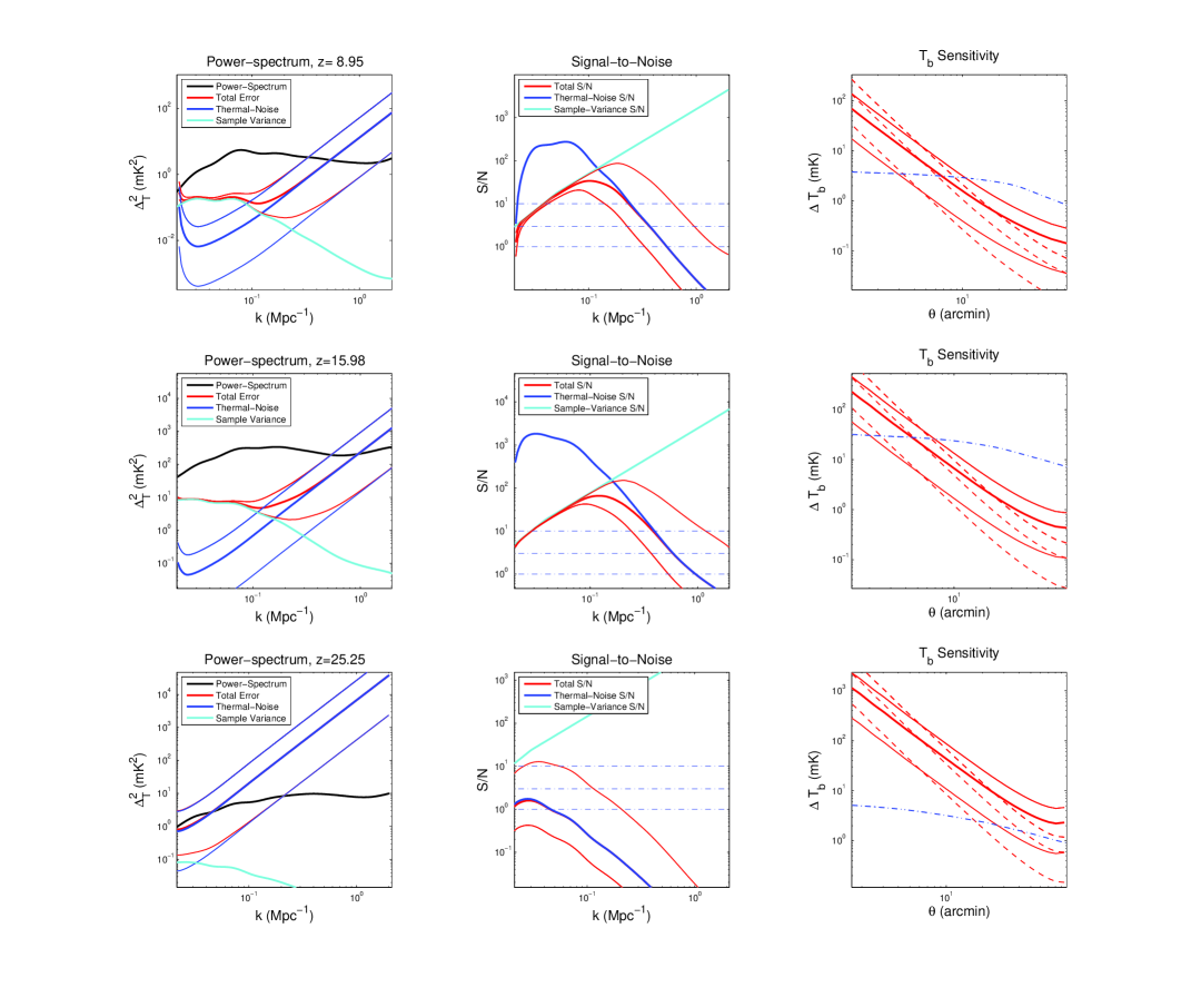
Figure 4: Rollout from half to four times SKA1: Idem to Fig.2 & 3. The solid red lines from bottom to top (middle column) show the S/N for a deep survey for $f_{\rm s}=0.5,1.0,4.0$. In the right column the brightness temperature (from bottom to top) is given for SKA2, SKA1 and half SKA1.

8 Summary, Conclusions and Highlights

SKA1-LOW and finally SKA2-LOW will be a transformational instrument in the study of the physics of the first stars, galaxies and black holes, dark-matter, the IGM, cosmology and possibly gravity during the first one billion years of the Universe, via statistical and direct measurements (e.g. power-spectra and tomography) of the redshifted 21-cm line from neutral hydrogen.

SKA1 will enable brightness temperature levels of $\sim$1 mK to be reached in 1000 hrs of integration (BW=1 MHz) from $z\sim 6$ to $z\sim 28$ ($>$50 MHz) over increasing angular scales ranging $\sim$5–300 arcminutes. SKA2 could potentially enable even higher redshift observations, starting to probe the late Dark Ages, as well as probe a much larger area of the sky (via multi-beaming) to a much greater depth in less time, reducing the thermal noise variance that will still limit SKA1 on the small scales where the dominant source population (e.g. mini-haloes) have their largest impact on neutral hydrogen (both via ionization and spin-temperature effects). The impact of SKA2 is expected in pushing tomography (i.e. direct imaging) to higher redshifts and to greater S/N (e.g. to probe redshift space distortions, higher order statistics, specific regions in the cubes, etc) where the sensitivity of SKA1 will still be insufficient. Although the Cosmic Dawn will be opened by SKA1, SKA2 will allow it to be studied in much great detail similar to the impact of SKA1 on the study of neutral hydrogen during the Epoch of Reionization.

We have outlined a three-tiered survey (deep and shallow/medium-deep and 21-cm absorption line measurements) with SKA1 that allow one to reach the goals of measuring the HI brightness temperature to a level of around 1 mK for tomography (a genuinely unique capability of SKA1 and SKA2) over a range of a few arc minutes up to a degree (depending on redshift), reduce sample variance and reach power-spectrum measurements up to one arcmin scales. Such a three tiered survey (assuming 21-cm absorption measurements can piggy-back on the deep survey) can be carried out in $3\times 2500$ hrs assuming that the full 300 MHz BW of SKA1 can be split in to two beams of 150 MHz. Such a survey is expected to take of order five years, assuming an efficiency of 50% of all night-time data (assuming 8-hr tracks) over such a period by selecting the best observing times and minimizing the impact of the ionosphere and emission from the Milky Way. This is not a project that can be carried out in a few months of full-time observations. Experience with the low-frequency SKA precursors and pathfinders confirms that good ”observing conditions” are necessary for a successful CD/EoR projects.

Finally, a three-tiered survey with SKA1-LOW is expected to generate strong synergy with other major (future) facilities such as JWST, ALMA, Euclid, as well as with (CO/CII) intensity-mapping arrays and large ground-based IR facilities such as the ELT. Many of the details can be found in the accompanying CD/EoR chapters in this volume.

8.1 SKA1 and 2 Science High-lights

Some high-light science results, in random order, expected to be largely unique for SKA1 (and 2) are given below. For each bullet point we refer to the first author of the related chapters in this volume:

• Direct imaging of ionized regions and HI fluctuations on scales of arcminutes and larger during the Epoch of Reionization and Cosmic Dawn — Mellema et al. 2015; Wyithe et al. 2015

• Probing many aspects of cosmology/cosmography out to the highest possible redshifts (i.e. $z=27$ in case of SKA1) — Pritchard et al. 2015

• Enabling one to probe $k\sim 1000$ Mpc^-1 scales via 21-cm absorption, probing mini-halos even out of reach of JWST — Ciardi et al. 2015

• Direct study of the state and chemistry of the IGM in the first billions years of the Universe – Ahn et al. 2015; Subrahmanyan et al. 2015

• Unique studies (i.e. CD) beyond the Epoch of Reionization which will remain out of reach of most of not all other (planned) facilities in particular of the first (Pop-III stars and X-ray heating sources) – Mesinger et al. 2015; Semelin et al. 2015

• Probing the impact of bulk-flows during the later Dark Ages and the Cosmic Dawn allowing physics during the Dark Ages and CMB to be probed in a unique manner – Maio et al. 2015

• Strong synergy with intensity mapping of the CO, CII, Lyman-$\alpha$ lines, possible molecular lines from primordial collapsing gas (e.g. H₂ and HD), as well as the kS-Z effect and NIR/X-ray mission, as well as with many other (planned) facilities in space and on the ground — Chang et al. 2015; Jelic et al. 2015

We conclude to say that direct detection of neutral hydrogen at high redshift, beyond the statistical approaches of current experiments, as well as probing the Cosmic Dawn will be defining abilities of the SKA (1 and 2). SKA can probe the universe back to 100 Myr after the Big Bang, well beyond even the limitations of JWST. This unique science can be carried out in a three-tiered survey of 7500 hrs or total on-sky time.

Appendix A Author Institutions

L.V.E Koopmans, Kapteyn Astronomical Institute, University of Groningen, The Netherlands
J. Pritchard, Imperial College, U.K.
G. Mellema, Dept. of Astronomy and Oskar Klein Centre, Stockholm Univ., Sweden
F. Abdalla, University College London, U.K.
J. Aguirre, University of Pennsylvania, USA
K. Ahn, Dept. of Earth Science, Chosun University, Korea
R. Barkana, Tel Aviv University, Israel
I. van Bemmel, Joint Institute for VLBI in Europe, The Netherlands
G. Bernardi, SKA South Africa & Rhodes University, South Africa
A. Bonaldi, Jodrell Bank Centre for Astrophysics, University of Manchester, U.K.
F. Briggs, Research School of Astronomy & Astrophysics, Australian National University
A.G. de Bruyn, Netherlands Institute for Radio Astronomy (ASTRON), The Netherlands
T.C. Chang, Academia Sinica Institute of Astronomy & Astrophysics, Taiwan
E. Chapman, Department of Physics & Astronomy, University College London, U.K.
X. Chen, National Astronomical Observatories, Chinese Academy of Science, Beijing, China
B. Ciardi, Max Planck Institute for Astrophysics, Garching, Germany
K.K. Datta, Dept. of Physics, Presidency University, Kolkata, India
P. Dayal, Institute for Computational Cosmology, Durham University, U.K.
A. Ferrara, Scuola Normale Superiore, Pisa, Italy
A. Fialkov, Ecole Normale Superieure, Paris, France
F. Fiore, INAF Osservatorio Astronomico di Roma, Italy
K. Ichiki, Nagoya University, Japan
I. T. Iliev, Astronomy Centre, Department of Physics & Astronomy, University of Sussex, U.K.
S. Inoue, Max Planck Institute for Astrophysics, Germany
V. Jelić, Kapteyn Astronomical Institute, University of Groningen, and ASTRON, The Netherlands
M. Jones, Oxford University, U.K.
J. Lazio, Jet Propulsion Laboratory, California Institute of Technology, USA
K. J. Mack, University of Melbourne, Australia
U. Maio, INAF-Trieste, Italy & Leibniz Institute for Astrophysics, Germany
S. Majumdar, Stockholm University, Sweden
A. Mesinger, Scuola Normale Superiore, Pisa, Italy
M.F. Morales, Dark Universe Science Center, University of Washington, USA
A. Parsons, University California Berkeley, USA
U.-L. Pen, Canadian Institute for Theoretical Astrophysics, Toronto, Canada
M. Santos, University of Western Cape, South Africa
R. Schneider, INAF/Osservatorio Astronomico di Roma, Italy
B. Semelin, LERMA, Observatoire de Paris, France
R.S. de Souza, MTA Eotvos University, Hungary
R. Subrahmanyan, Raman Research Institute, Bangalore 560080, India
T. Takeuchi, Nagoya University, Japan
C. Trott, International Centre for Radio Astronomy Research, Curtin University, Australia
H. Vedantham, Kapteyn Astronomical Institute, University of Groningen, The Netherlands
J. Wagg, Square Kilometre Array Organisation
R. Webster, School of Physics, University of Melbourne, Australia
S. Wyithe, School of Physics, University of Melbourne, Australia

References

- Ahnet al. (2015) Ahn, K., et al., 2015, “Probing the First Galaxies and Their Impact on the Intergalactic Medium through 21-cm Observations of the Cosmic Dawn with the SKA”, in proceedings of “Advancing Astrophysics with the Square Kilometre Array”, PoS(AASKA14)003
- Ali et al. (2015) Ali, Z. S., Parsons, A. R., Zheng, H., et al. 2015, ArXiv e-prints
- Ali-Haïmoud et al. (2014) Ali-Haïmoud, Y., Meerburg, P. D., & Yuan, S. 2014, Phys Rev D, 89, 083506
- Barkana & Loeb (2001) Barkana, R., & Loeb, A. 2001, Physics Reports, 349, 125
- Becker et al. (2001) Becker, R. H., Fan, X., White, R. L., et al. 2001, AJ, 122, 2850
- Bolton et al. (2010) Bolton, J. S., Becker, G. D., Wyithe, J. S. B., Haehnelt, M. G., & Sargent, W. L. W. 2010, MNRAS, 406, 612
- Bouwens et al. (2012) Bouwens, R. J., Illingworth, G. D., Oesch, P. A., et al. 2012, ApJL, 752, L5
- Braun (2014) Braun, R., 2014, “SKA1 Array Configurations”, Document Number SKA-OFF.AG.CNF-SKO-TN-001 Revision 1, SKA Organisation
- Carilli et al. (2002) Carilli, C. L., Gnedin, N. Y., & Owen, F. 2002, ApJ, 577, 22
- Cooray et al. (2008) Cooray, A., Li, C., & Melchiorri, A. 2008, Phys Rev D, 77, 103506
- Changet al. (2015) Chang, T.C., et al., 2015, “Synergy of CO/[CII]/Lya Line Intensity Mapping with the SKA”, in proceedings of “Advancing Astrophysics with the Square Kilometre Array”, PoS(AASKA14)004
- Chapmanet al. (2015) Chapman, E., et al., 2015, “Cosmic Dawn and Epoch of Reionization Foreground Removal with the SKA”, in proceedings of “Advancing Astrophysics with the Square Kilometre Array”, PoS(AASKA14)005
- Ciardiet al. (2015) Ciardi, B., et al., 2015, “21-cm forest with the SKA”, in proceedings of “Advancing Astrophysics with the Square Kilometre Array”, PoS(AASKA14)006
- Davé et al. (2006) Davé, R., Finlator, K., & Oppenheimer, B. D. 2006, MNRAS, 370, 273
- de Souza et al. (2013) de Souza, R. S., Ishida, E. E. O., Johnson, J. L., Whalen, D. J., & Mesinger, A. 2013, MNRAS, 436, 1555
- de Souza et al. (2014) de Souza, R. S., Ishida, E. E. O., Whalen, D. J., Johnson, J. L., & Ferrara, A. 2014, MNRAS, 442, 1640
- Dijkstra (2006) Dijkstra, M. 2006, New Astronomy Reviews, 50, 204
- Dillon et al. (2014) Dillon, J. S., Liu, A., Williams, C. L., et al. 2014, Phys Rev D, 89, 023002
- Ellis et al. (2013) Ellis, R. S., McLure, R. J., Dunlop, J. S., et al. 2013, ApJL, 763, L7
- Fan et al. (2002) Fan, X., Narayanan, V. K., Strauss, M. A., et al. 2002, AJ, 123, 1247
- Fan et al. (2006) Fan, X., Strauss, M. A., Becker, R. H., et al. 2006, AJ, 132, 117
- Fernandez & Zaroubi (2013) Fernandez, E. R., & Zaroubi, S. 2013, MNRAS, 433, 2047
- Fialkov et al. (2015) Fialkov, A., Barkana, R., & Cohen, A. 2015, Physical Review Letters, 114, 101303
- Fialkov et al. (2014a) Fialkov, A., Barkana, R., Pinhas, A., & Visbal, E. 2014a, MNRAS, 437, L36
- Fialkov et al. (2014b) Fialkov, A., Barkana, R., & Visbal, E. 2014b, Nature, 506, 197
- Fialkov & Loeb (2013) Fialkov, A., & Loeb, A. 2013, Journal of Cosmology and Astroparticle Physics, 11, 66
- Field (1958) Field, G. B. 1958, Proceedings of the IRE, 46, 240
- Field (1959) —. 1959, ApJ, 129, 536
- Furlanetto & Briggs (2004) Furlanetto, S. R., & Briggs, F. H. 2004, New Astronomy Reviews, 48, 1039
- Greenhill et al. (2014) Greenhill, L. J., Kocz, J., Barsdell, B. R., Clark, M. A., & LEDA Collaboration. 2014, in Exascale Radio Astronomy, 10301
- Harker et al. (2009) Harker, G. J. A., Zaroubi, S., Thomas, R. M., et al. 2009, MNRAS, 393, 1449
- Helgason et al. (2014) Helgason, K., Cappelluti, N., Hasinger, G., Kashlinsky, A., & Ricotti, M. 2014, ApJ, 785, 38
- Ilievet al. (2015) Iliev, I., et al., 2015, “Epoch of Reionization modelling and simulations for SKA”, in proceedings of “Advancing Astrophysics with the Square Kilometre Array”, PoS(AASKA14)007
- Jelicet al. (2015) Jelic, V., et al., 2015, “SKA - EoR correlations and cross-correlations: kSZ, radio galaxies, and NIR background”, in proceedings of “Advancing Astrophysics with the Square Kilometre Array”, PoS(AASKA14)008
- Lewis & Challinor (2007) Lewis, A., & Challinor, A. 2007, Phys Rev D, 76, 083005
- Loeb & Furlanetto (2013) Loeb, A., & Furlanetto, S. R. 2013, The First Galaxies in the Universe
- Lorenzoni et al. (2011) Lorenzoni, S., Bunker, A. J., Wilkins, S. M., et al. 2011, MNRAS, 414, 1455
- Madau et al. (1997) Madau, P., Meiksin, A., & Rees, M. J. 1997, ApJ, 475, 429
- Maioet al. (2015) Maio, U., et al., 2015, “Bulk Flows and End of the Dark Ages with the SKA”, in proceedings of “Advancing Astrophysics with the Square Kilometre Array”, PoS(AASKA14)009
- Matthee et al. (2014) Matthee, J. J. A., Sobral, D., Swinbank, A. M., et al. 2014, MNRAS, 440, 2375
- McQuinn et al. (2006) McQuinn, M., Zahn, O., Zaldarriaga, M., Hernquist, L., & Furlanetto, S. R. 2006, ApJ, 653, 815
- Mellema et al. (2013) Mellema, G., Koopmans, L. V. E., Abdalla, F. A., et al. 2013, Experimental Astronomy, 36, 235
- Mellemaet al. (2015) Mellema, G., et al., 2015, “HI tomographic imaging of the Cosmic Dawn and Epoch of Reionization with SKA”, in proceedings of “Advancing Astrophysics with the Square Kilometre Array”, PoS(AASKA14)010
- Mesinger (2010) Mesinger, A. 2010, MNRAS, 407, 1328
- Mesinger et al. (2014) Mesinger, A., Ewall-Wice, A., & Hewitt, J. 2014, MNRAS, 439, 3262
- Mesingeret al. (2015) Mesinger, A., et al., 2015, “Constraining the Astrophysics of the Cosmic Dawn and the Epoch of Reionization with the SKA”, in proceedings of “Advancing Astrophysics with the Square Kilometre Array”, PoS(AASKA14)011
- Morales & Wyithe (2010) Morales, M. F., & Wyithe, J. S. B. 2010, Ann. Rev. Astron.& Astrophys. , 48, 127
- Mortlock et al. (2011) Mortlock, D. J., Warren, S. J., Venemans, B. P., et al. 2011, Nature, 474, 616
- Novaco & Brown (1978) Novaco, J. C., & Brown, L. W. 1978, ApJ, 221, 114
- Paciga et al. (2011) Paciga, G., Chang, T.-C., Gupta, Y., et al. 2011, MNRAS, 413, 1174
- Pacucci et al. (2014) Pacucci, F., Mesinger, A., Mineo, S., & Ferrara, A. 2014, MNRAS, 443, 678
- Patra et al. (2013) Patra, N., Subrahmanyan, R., Raghunathan, A., & Udaya Shankar, N. 2013, Experimental Astronomy, 36, 319
- Patra et al. (2015) Patra, N., Subrahmanyan, R., Sethi, S., Udaya Shankar, N., & Raghunathan, A. 2015, ApJ, 801, 138
- Pillepich et al. (2007) Pillepich, A., Porciani, C., & Matarrese, S. 2007, ApJ, 662, 1
- Pober et al. (2015) Pober, J. C., Ali, Z. S., Parsons, A. R., et al. 2015, ArXiv e-prints
- Pritchard & Loeb (2008) Pritchard, J. R., & Loeb, A. 2008, Phys Rev D, 78, 103511
- Pritchardet al. (2015) Pritchard, J., et al., 2015, “Cosmology from EoR/Cosmic Dawn with the SKA”, in proceedings of “Advancing Astrophysics with the Square Kilometre Array”, PoS(AASKA14)012
- Ripamonti et al. (2010) Ripamonti, E., Iocco, F., Ferrara, A., et al. 2010, MNRAS, 406, 2605
- Robertson et al. (2010) Robertson, B. E., Ellis, R. S., Dunlop, J. S., McLure, R. J., & Stark, D. P. 2010, Nature, 468, 49
- Robertson et al. (2015) Robertson, B. E., Ellis, R. S., Furlanetto, S. R., & Dunlop, J. S. 2015, ApJL, 802, L19
- Ruiz-Velasco et al. (2007) Ruiz-Velasco, A. E., Swan, H., Troja, E., et al. 2007, ApJ, 669, 1
- Semelinet al. (2015) Semelin, B., et al., 2015, “The physics of Reionization: processes relevant for SKA observations”, in proceedings of “Advancing Astrophysics with the Square Kilometre Array”, PoS(AASKA14)013
- Simcoe et al. (2012) Simcoe, R. A., Sullivan, P. W., Cooksey, K. L., et al. 2012, Nature, 492, 79
- Smoot et al. (1992) Smoot, G. F., Bennett, C. L., Kogut, A., et al. 1992, ApJL, 396, L1
- Sobacchi & Mesinger (2014) Sobacchi, E., & Mesinger, A. 2014, MNRAS, 440, 1662
- Sparre et al. (2014) Sparre, M., Hartoog, O. E., Krühler, T., et al. 2014, ApJ, 785, 150
- Stacy & Bromm (2013) Stacy, A., & Bromm, V. 2013, MNRAS, 433, 1094
- Subrahmanyanet al. (2015) Subramanyan, R., et al., 2015, “All-sky signals from recombination to reionization with the SKA”, in proceedings of “Advancing Astrophysics with the Square Kilometre Array”, PoS(AASKA14)014
- Taoso et al. (2008) Taoso, M., Bertone, G., Meynet, G., & Ekström, S. 2008, Phys Rev D, 78, 123510
- Theuns et al. (2002) Theuns, T., Zaroubi, S., Kim, T.-S., Tzanavaris, P., & Carswell, R. F. 2002, MNRAS, 332, 367
- Trott (2014) Trott, C. M. 2014, PASA, 31, 26
- Tseliakhovich & Hirata (2010) Tseliakhovich, D., & Hirata, C. 2010, Phys Rev D, 82, 083520
- Valdés et al. (2013) Valdés, M., Evoli, C., Mesinger, A., Ferrara, A., & Yoshida, N. 2013, MNRAS, 429, 1705
- van Haarlem et al. (2013) van Haarlem, M. P., Wise, M. W., Gunst, A. W., et al. 2013, A.&A, 556, A2
- Wouthuysen (1952) Wouthuysen, S. A. 1952, AJ, 57, 31
- Wyitheet al. (2015) Wyithe, S., et al., 2015, “Imaging HII Regions from Galaxies and Quasars During Reionisation with SKA”, in proceedings of “Advancing Astrophysics with the Square Kilometre Array”, PoS(AASKA14)015
- Yatawatta et al. (2013) Yatawatta, S., de Bruyn, A. G., Brentjens, M. A., et al. 2013, A.&A, 550, A136
- Zemcov et al. (2014) Zemcov, M., Smidt, J., Arai, T., et al. 2014, Science, 346, 732