Electric Characteristics of Rotational States positive parity in isotopes ${}^{170,172,174}Yb$

Abstract

Accounting for Coriolis mixing of experimentally known rotational bands with $K^{\pi}<3^{+}$, non-adiabatic effects in energy and electric characteristics of excited states are investigated, within phenomenological model.

The energy and wave function structure of excited states are calculated. The finding reveals that the bands mixing has been found to have considerable impact on the wave function of low-lying states $0^{+}$ and $2^{+}$ bands.

In addition, the probabilities of $E2$– transitions have been calculated. The values from calculations of $B(E2)$– transitions from $0_{2}^{+}$, $0_{3}^{+}$, $2_{1}^{+}$, and $2_{2}^{+}$ bands are compared with the experimental data.

I Introduction

Despite the fact that the structure of deformed nuclei and nature of low excited levels have been substantially studies over more than four decades, this still occupies a central part of today’s research Bohr -Burke .

An extensive research interest in the properties of deformed nuclei has risen in recent years with the exploration of a new collective isovector magnetic dipole mode Bohle ; Zilges . The measured values of excited energy of magnetic mode are found to be not so high in an excited spectrum, and consideration of mixing with low-lying exciting states appear to lead to an interesting physical phenomena Usmanov ; Usmanov2010 .

The nuclei ${}^{170,172,174}Yb$ have been well studied. It is important to note that these are investigated in a number of ways such as radioactive decay of ${}^{170,172,174}Lu$, and different nuclear reactions. In these isotopes, many $1^{+}$ states and $K^{\pi}=0^{+},2^{+}$ bands have been observed. For instance, the excited energy $K^{\pi}=0^{+}$ and $2^{+}$ it rises with the increase in number of neutrons (see Figure 1).

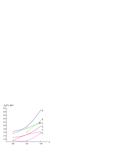
Figure 1: (Color online) The energy of $I=2$ states of $K^{\pi}=0_{2}^{+},0_{3}^{+},0_{4}^{+},0_{5}^{+},2_{1}^{+}$ and $2_{2}^{+}$ bands in isotopes ${}^{170,172,174}Yb$.

The values of probability of $B(E2)$ with low-lying levels of $K^{\pi}=0^{+}$, $2^{+}$ bands, and also Rasmusson’s parameter value $X_{I}(E0/E2)$, dimensionless units matrix element $\rho(E0)$ for the $E0$– transition and a multipole mixture coefficients $\delta(E2/M1)$ are defined experimentally Baglin -Browne .

Numerous conducted experiments on defining spectroscopic characteristics of low-lying exciting states, particular $K^{\pi}=1^{+}$ in deformed nuclei Zilges , have motivated the further theoretical investigations. In this case, investigations influence of $K^{\pi}=1^{+}$ states to the properties of low-lying levels is actual.

Present paper focuses on low-lying states of positive parity of isotopes ${}^{170,172,174}Yb$. The calculation are conducted by utilizing a phenomenological model Usmanov which accounts Coriolis mixture all of the experimentally known low-lying rotational bands states with $K^{\pi}<3^{+}$.

Experimentally observed $K$– forbidden transitions as well as nonadiabaticities of energy and in ratios of $E2$– transitions can be explained by Coriolis mixture states.

II The Model

To analyze the properties of low-lying positive parity states in $Yb$ isotopes, the phenomenological model of Usmanov is exploited. This model takes into account the mixing of states of the $K^{\pi}=0^{+},2^{+}$ and $1^{+}$ bands. The Hamiltonian model is

$$H=H_{rot}(I^{2})+H_{K,K^{\prime}}$$ (1)

$$H_{{}_{K^{\prime}K}}^{\sigma}(I)=\omega_{{}_{K}}\delta_{{}_{K,K^{\prime}}}-\omega_{rot}(I)(j_{x})_{{}_{K,K^{\prime}}}\zeta(I,K)\delta_{{}_{K,K^{\prime}\pm 1}}$$ (2)

where $\omega_{{}_{K}}$– bandhead energy of rotational band, $\omega_{rot}(I)$– an angular frequency of rotational nucleus, $(j_{x})_{{}_{K,K^{\prime}}}$– matrix elements which describe Coriolis mixture between rotational bands and

$$\zeta(I,0)=1\ \ \ \ \ \zeta(I,2)=\left[1-\frac{2}{I(I+1)}\right]^{\frac{1}{2}}$$

The eigenfunction of Hamiltonian model (1) is

$$|IMK> = \sqrt{\frac{2I+1}{16\pi^{2}}}\left\{\sqrt{2}\Psi_{gr,K}^{I}D_{MK}^{I}(\theta)\right.$$

$$+ \left.\sum_{K^{\prime}}\frac{\Psi_{K^{\prime},K}^{I}}{\sqrt{1+\delta_{K^{\prime},0}}}\left[D_{M,K^{\prime}}^{I}(\theta)b_{K^{\prime}}^{+}\right.\right.$$

$$+ \left.\left.(-1)^{I+K^{\prime}}D_{M,-K^{\prime}}^{I}(\theta)b_{-K^{\prime}}^{+}\right]\right\}|0>$$

here $\Psi_{K^{\prime},K}^{I}$ is the amplitude of mixture of basis states.

The rotational part of Hamiltonian (1) $H_{rot}(I)$ is diagonal by wave functions (II). Note that $H_{rot}(I)$ is determined by exploiting Harris parameterization for energy and angular momentum Harris

$$E_{rot}(I)=\frac{1}{2}\Im_{0}\omega_{rot}^{2}(I)+\frac{3}{4}\Im_{1}\omega_{rot}^{4}(I)$$ (4)

$$\left[I(I+1)\right]^{1/2}=\Im_{0}\omega_{rot}(I)+\Im_{1}\omega_{rot}^{3}(I)$$ (5)

where $\Im_{0}$ and $\Im_{1}$– are the inertia parameters of the rotational core.

The rotational frequency of the core $\omega_{rot}(I)$ is found by solving cubic equation (5). This equation has two imaginary roots and one real root. The real root is as follows

$$\omega_{rot}(I) = \left\{\frac{\widetilde{I}}{2\Im_{1}}+\left(\left(\frac{\widetilde{I}}{2\Im_{1}}\right)^{2}+\left(\frac{\Im_{0}}{3\Im_{1}}\right)^{3}\right)^{\frac{1}{2}}\right\}^{\frac{1}{3}}$$

$$+ \left\{\frac{\widetilde{I}}{2\Im_{1}}-\left(\left(\frac{\widetilde{I}}{2\Im_{1}}\right)^{2}+\left(\frac{\Im_{0}}{3\Im_{1}}\right)^{3}\right)^{\frac{1}{2}}\right\}^{\frac{1}{3}}$$

where $\widetilde{I}=\sqrt{I(I+1)}$. Equation (II) gives $\omega_{rot}(I)$ at the given spin $I$ of the core.

Solving the Shrödinger equation

$$H_{K,K^{\prime}}^{\sigma}\Psi_{K,K^{\prime}}^{I}=\mathcal{E}_{K}(I)\Psi_{K,K^{\prime}}^{I}.$$ (7)

we define eigne function and energy of a Hamiltonian. The total energy of state is defined by

$$E_{K}(I)=E_{rot}(I)+\mathcal{E}_{K}(I)$$ (8)

II.1 Energy spectra and structures of the states

The calculations have been carried out for the isotopes ${}^{170,172,174}Yb$. All experimentally known rotational bands of positive parity with $K^{\pi}<3^{+}$ have been included in basis Hamiltonian states.

The experiment suggests that $m=5$ band with $K^{\pi}=0_{m}^{+}$, one band $\ell=1$ with $K^{\pi}=2_{\ell}^{+}$, and $\nu=19$ with $K^{\pi}=1_{\nu}^{+}$ states in ${}^{170}Yb$ Baglin . These all $n=m+\ell+\nu=25$ rotational bands have been included in the basis states of Hamiltonian (1). For the isotopes ${}^{172,174}Yb$, basis states of Hamiltonian include $n=15$ ($m=5$, $\ell=2$ and $\nu=8$) and $n=22$ ($m=5$, $\ell=2$ and $\nu=15$), correspondingly Zilges ; Singh ; Browne .

The parameters of inertia $\Im_{0}$ and $\Im_{1}$ are estimated by exploiting Harris parameterization (4), and using the experimental data for energy up to spin $I\leq 8\hbar$ for ground band Okhunov .

The Hamiltonian (2) has transformational properties, that the state (II) can be classified as quantum number — $\sigma=\pm 1$ signature, which imposes restrictions on angular momentum values.

$$(-1)^{I}\sigma=1.$$

For the states with negative signature $\sigma=-1$, Hamiltonian (2) has dimension $n=\ell+\nu$, as in bands with $K^{\pi}=0_{m}^{+}$ the are no condition states with odd spins $I$. For the states with positive signature $\sigma=+1$, Hamiltonian (2) has dimension $n=m+\ell+\nu$.

The model parameters are described as follows:

a) the bandhead energy ground $\omega_{0_{1}}$ and $K^{\pi}=0_{m}^{+}$ bands has taken from experiment, as they are not revolted by Coriolis force. Bandhead energy of $1_{\nu}^{+}$ bands are also defined from an experiment Zilges ; Baglin

$$\omega_{1_{\nu}}=E_{1_{\nu}}^{exp.}(I=1)-E_{rot}(I=1);$$

b) matrix elements $(j_{x})_{2_{\ell}1}=(j_{x})_{2_{\ell}1_{\nu}}$ and bandhead energy of $2_{\ell}^{+}$– bands $\omega_{2_{\ell}}$ are determined from the most favored experimental and theoretical spectrum of energy states with a negative signature $\sigma=-1$, e.a. for energy state for even spins $I$;

c) the matrix elements $(j_{x})_{0_{m}1}=(j_{x})_{0_{m}1_{\nu}}$ defined by the least square method from the best fitted of theoretical energy spectra state with positive signature $\sigma=+1$ with experimental data.

The obtained values of model parameters are presented in Table 1.

Table 1: Parameters used in the calculations for the isotopes ${}^{170,172,174}Yb$

$A$	$(j_{x})_{0_{1},1_{\nu}}$	$(j_{x})_{0_{2},1}$	$(j_{x})_{0_{3},1}$	$(j_{x})_{0_{4},1}$	$(j_{x})_{0_{5},1}$	$(j_{x})_{2_{1},1}$	$(j_{x})_{2_{2},1}$
$170$	0.1864	0.3936	0.6586	0.9081	0.0009	0.7278	–
$172$	0.2754	0.9777	0.7176	0.11	0.30	0.325	0.21
$174$	0.185	0.4	0.25	0.15	0.20	0.085	0.1

Note: $(j_{x})_{{}_{K^{\prime},K}}$– are matrix elements of the Coriolis interactions.

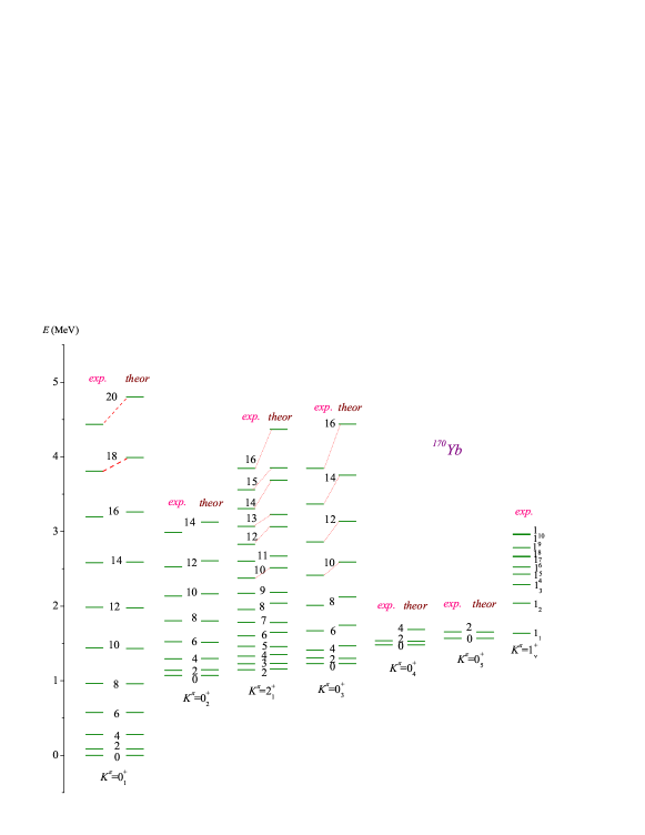
Figure 2: (Color online) Comparison of the calculated and experimental energy spectra of positive-parity states for ${}^{170}Yb$.

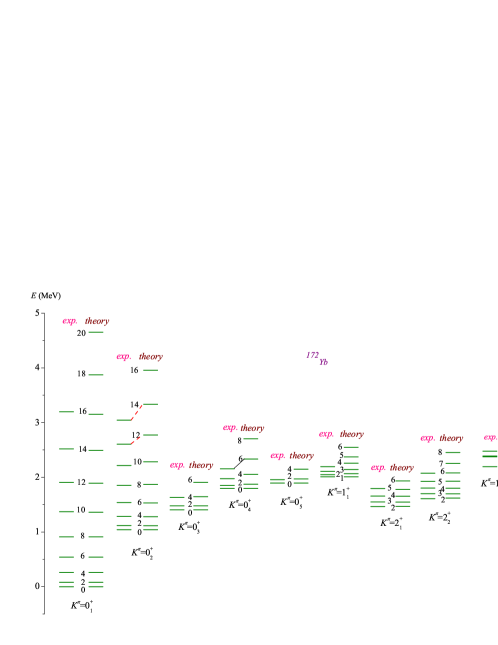
Figure 3: (Color online) Comparison of the calculated and experimental energy spectra of positive-parity states for ${}^{172}Yb$.

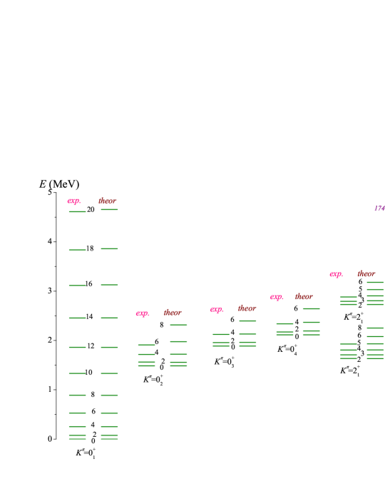
Figure 4: (Color online) Comparison of the calculated and experimental energy spectra of positive-parity states for ${}^{174}Yb$.

Calculation comparison of energy with experimental values for ${}^{170,172,174}Yb$ is illustrated in Figures 2,3 and 4, correspondingly.

Apparently, one may see from the Figures that the model qualitatively reproduces experimental energy of rotational states up to energy $3MeV$. However, in high spin values $I\geq 12\hbar$ noticeable deviation has been observed in calculated values of energy and that obtained from experiment. Note that this deviation increases with the growth of angular momentum $I$. This is probably due to the fact that the influence of rotation on internal nuclei structure has not been considered in this model. In future, we will study electromagnetic properties of low-lying states $I<10\hbar$.

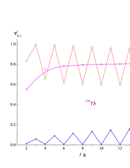
Figure 5: (Color online) Structure of the wave-functions of $2_{1}^{+}$– band states for ${}^{170}Yb$.

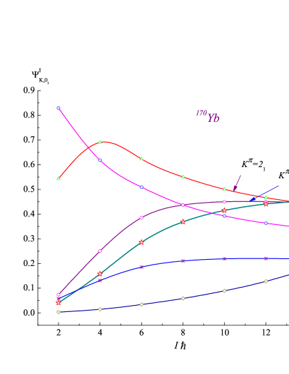
Figure 6: (Color online) Structure of the wave-functions of $0_{2}^{+}$– band states for ${}^{170}Yb$.

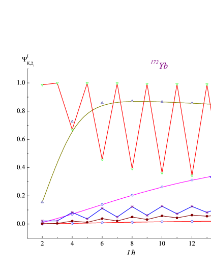
Figure 7: (Color online) Structure of the wave-functions of $2_{1}^{+}$– band states for ${}^{172}Yb$.

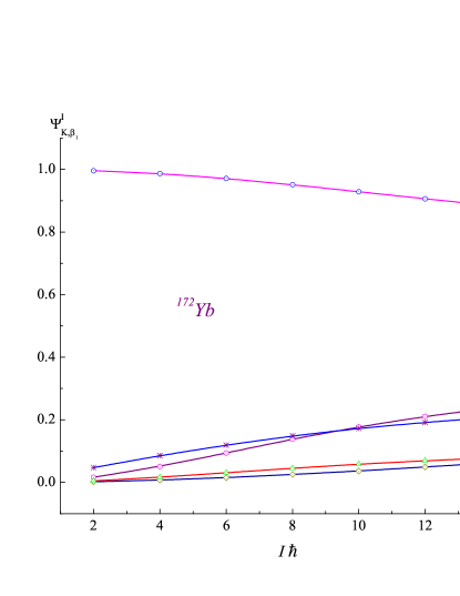
Figure 8: (Color online) Structure of the wave-functions of $0_{2}^{+}$– band states for ${}^{172}Yb$.

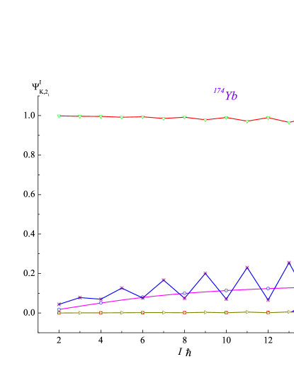
Figure 9: (Color online) Structure of the wave-functions of $2_{1}^{+}$– band states for ${}^{174}Yb$.

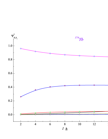
Figure 10: (Color online) Structure of the wave-functions of $0_{2}^{+}$– band states for ${}^{174}Yb$.

Amplitude of the states $\Psi_{K^{{}^{\prime}},K}$ for $K^{\pi}=2_{1}^{+}$– and $0_{2}^{+}$– bands for ${}^{170,172,174}Yb$, are provided in Figures 5, 6, 7, 8, 9 and 10, respectively. The components which have small values are not illustrated in Figure. Also the components $\Psi_{1_{\nu},K}$ band are not given except for the first $1_{1}^{+}$. The values for others $\Psi_{1_{\nu}^{+},K}$ states are define as follows

$$\Psi_{1_{\nu},K}=\Psi_{1_{1},K}\frac{\omega_{1_{1}}-\omega_{K}}{\omega_{1_{\nu}}-\omega_{K}}.$$ (9)

From Figures 5 and 7, we can see that $K^{\pi}=0_{2}^{+}$ and $K^{\pi}=2_{1}^{+}$ bands states in ${}^{170}Yb$, $K^{\pi}=0_{3}^{+}$ and $K^{\pi}=2_{1}^{+}$ bands in ${}^{172}Yb$ are mixed strongly even in low spin values $I$. It is associated with the close location to each other (see Figure 1). In isotopes ${}^{170,172}Yb$, considerable deviation in signature of the states $K^{\pi}=2_{1}^{+}$ band can be observed. This reflects in the values of probability electromagnetic transitions. In this case, description of quantum number $K$ is difficult for these states. Thus, in ${}^{170}Yb$, a number of research works Begzhanov in this context note that the states with $I=2^{+}$ (1.1386 MeV) and $I=2^{+}$ (1.1454 MeV) $K=2$ and $K=0$, respectively. On the other hand, some works Baglin document that $K=0$ and $K=2$, correspondingly. In case ${}^{174}Yb$, the mixture effect is not so strong.

III Electric Quadrupole transitions

With the wave functions calculated by solving the Shrödinger equation (7), reduced probabilities of $E2$– transitions between states $I_{i}K_{i}$ and states of ground band $I_{f}0_{1}$ are calculated Usmanov .

$$B(E2;I_{i}K_{i}\rightarrow I_{f}0_{1}) = \left\{\sqrt{\frac{5}{16\pi}}eQ_{0}\left[\Psi_{0_{1},0_{1}}^{I_{f}}\Psi_{0_{1},K_{i}}^{I_{i}}C_{I_{i}0;20}^{I_{f}0}+\sum_{n}\Psi_{K_{n},0_{1}}^{I_{f}}\Psi_{K_{n},K_{i}}^{I_{i}}C_{I_{i}K_{n};20}^{I_{f}K_{n}}\right]\right.$$ (10)

$$+ \left.\sqrt{2}\left[\Psi_{0_{1},0_{1}}^{I_{f}}\sum_{n}\frac{(-1)^{K_{n}}m_{{}_{K_{n}}}\Psi_{K_{n},K_{i}}^{I_{i}}}{\sqrt{1+\delta_{K_{n},0}}}C_{I_{i}K_{n};2-K_{n}}^{I_{f}0}+\Psi_{0_{1},K_{i}}^{I_{i}}\sum_{n}\frac{m_{{}_{K_{n}}}\Psi_{K_{n},0_{1}}^{I_{f}}}{\sqrt{1+\delta_{K_{n},0}}}C_{I_{i}0;2K_{n}}^{I_{f}K_{n}}\right]\right\}^{2}$$

here $m_{{}_{K_{n}}}=<0_{1}^{+}|\hat{m}(E2)|K_{n}^{+}>$– is matrix elements between intrinsic wave functions of ground $(0_{1}^{+})$ and $K_{n}^{+}=0_{m}^{+},2_{\ell}^{+},1_{\nu}^{+}$ bands which has a value obtained from experimental data, $Q_{0}$– is nuclear intrinsic quadrupole moment; and $C_{I_{i}K_{i};2(K_{i}+K_{1})}^{I_{f}K_{f}}$– Clebsch-Gordan coefficient.

For the reduced probabilities of $E2$– transitions from the $I=2$ state we have following equation in adiabatic approximation:

$$B^{adia}(E2;2K_{n}\rightarrow 00_{1})=$$ (11)

$$=\left(2-\delta_{K_{n},0}\right)|m_{{}_{K_{n}}}C_{2K_{n};2-K_{n}}^{00}|^{2}$$

which allows us to identify $m_{{}_{K_{n}}}$ parameter from the experimental data.

The $K^{\pi}=0_{2}^{+}$, $0_{3}^{+}$ and $2_{1}^{+}$ bands are very close to each other in isotopes ${}^{170,172}Yb$, which leads to a strong mixing of states even $I=2$. In this case, the adiabatic approximation (11) becomes inapplicable to determine $m_{{}_{K_{i}}}$.

The magnitude and sign parameters $m_{1_{1}}=m_{1_{\nu}}$ and $m_{2_{\ell}^{+}}$ are obtained form the best fitted ratio probabilities $R_{IK}=B(E2;IK\rightarrow I+10_{1})/B(E2;IK\rightarrow I-10_{1})$ and odd states of $K^{\pi}=2_{\ell}^{+}$ and $1_{\nu}^{+}$ bands. In addition, the most favored ratio $R_{IK}$ and even states (for the positive signature $\sigma=+1$) help to identify parameters $m_{0_{m}}$.

Table 2 reports $m_{{}_{K}}$ parameters which have been used in calculation $E2$– transitions.

Table 2: The values of the parameters $m_{K}$ and the intrinsic quadrupole moment $Q_{0}$, which are used in calculations (in $efm^{2}$)

$A$	$m_{0_{2}}$	$m_{0_{3}}$	$m_{0_{4}}$	$m_{0_{5}}$	$m_{1_{\nu}}$	$m_{2_{1}}$	$m_{2_{2}}$	$Q_{0}$Begzhanov
$170$	2	24	3	8	-5	19	8	780(4)
$172$	10	1	-6.9	-8	-5	15	-8	791(4)
$174$	8	1	-6.9	8	-10 ($m_{1_{1}}$=-1.7)	15	8	782(4)

Table 3 compares reduced probability $E2$– transitions with existing experimental data Baglin -Browne , Reich . Moreover, reduced matrix elements of $E2$– transitions for ${}^{172}Yb$ are provided in Table 4. In a similar vein, these values are also compared with experimental values as well as values found by using other models Fahlander -Arima .

Table 3: Reduced probability of $E2$– transitions in the isotopes $Yb$ ($e^{2}fm^{4}$)

A	$I_{i}K_{i}\rightarrow I_{f}K_{f}$	Exp.	Theory	$I_{i}K_{i}\rightarrow I_{f}K_{f}$	Exp.	Theory
${}^{170}Yb$	$22_{1}\rightarrow 00_{1}$	151(35)Baglin	90	$00_{3}\rightarrow 20_{1}$	60(15)Baglin	43
	$\rightarrow\ 20_{1}$	269(60)Baglin	60	$00_{4}\rightarrow 20_{1}$	567(118)Baglin	567
	$\rightarrow\ 40_{1}$	27(6)Baglin	10
${}^{172}Yb$	$22_{1}\rightarrow 00_{1}$	75.6(63)Singh ; 74.6(57)Reich	82	$00_{2}\rightarrow 20_{1}$	205(60)Singh	100
	$\rightarrow\ 20_{1}$	121(12)Reich	130	$20_{2}\rightarrow 00_{1}$	14(1)Singh ;    14(1)Reich	13
	$\rightarrow\ 40_{1}$	7.3(6)Singh ;    6.8(7)Reich	8.6	$\rightarrow\ 20_{1}$	45(7)Singh ;    52(8)Reich	23
	$42_{1}\rightarrow 20_{1}$	398(284)Singh	15	$\rightarrow\ 40_{1}$	142(20)Singh ; 140(20)Reich	74
	$\rightarrow\ 40_{1}$	739(512)Singh	81	$00_{3}\rightarrow 20_{1}$	0.14(3)Singh	1
	$32_{1}\rightarrow 20_{1}$	152(11)Reich	154	$20_{3}\rightarrow 00_{1}$	0.4(1)Singh ;    3.4(2)Reich	3.6
	$\rightarrow\ 40_{1}$	79(6)Reich	73	$\rightarrow\ 20_{1}$	0.6(4)Singh ;  11.9(8)Reich	3.0
	$22_{2}\rightarrow 00_{1}$	20(4)Singh ;    32(4)Reich	23	$\rightarrow\ 40_{1}$	1.0(1)Reich	1.2
	$\rightarrow\ 20_{1}$	31(2)Singh ;    51(7)Reich	38	$00_{4}\rightarrow 20_{1}$	$>$0.25Singh	48
	$\rightarrow\ 40_{1}$	3.3(4)Reich	2.2	$20_{4}\rightarrow 00_{1}$	10(6)Singh	12
	$32_{2}\rightarrow 20_{1}$	54(7)Reich	42	$00_{5}\rightarrow 20_{1}$	$>$ 0.27Singh	64
	$\rightarrow\ 40_{1}$	22(3)Reich	21	$20_{5}\rightarrow 00_{1}$	19(9)Singh	21
				$\rightarrow\ 20_{1}$	$>$ 0.18Singh	23
${}^{174}Yb$	$00_{2}\rightarrow 20_{1}$	$81_{-29}^{+64}$Browne	64	$22_{1}\rightarrow 20_{1}$	144(30)Browne	133

It is important to note that our results are obtained consecutively. In the initial step, energy and wave function the states are computed. Further, by utilizing these wave functions, reduced probability of $E2$– transitions are calculated. From the Table 4, one may gather that performed calculations within our model provide a better correspondence with experiment data.

Table 4: Reduced Matrix Elements of $E2$– transitions in ${}^{172}Yb$, calculated within our model which comparison with experimental data Fahlander and are calculated using the rotational-vibrational model (RVM2) Faessler and the IBA-1 model Arima $(eb)$

$I_{i}K_{i}\rightarrow I_{f}K_{f}$	Exp.	RVM2	IBA-1	Theory	$I_{i}K_{i}\rightarrow I_{f}K_{f}$	Exp.	RVM2	IBA-1	Theory
$20_{1}\rightarrow 20_{1}$	-2.63${}_{-0.27}^{+0.28}$	-2.92	-2.92	-2.93	$20_{1}\rightarrow 00_{1}$	2.45${}_{-0.12}^{+0.12}$	2.45a)	2.45a)	2.45a)
$40_{1}\rightarrow 40_{1}$	-3.54${}_{-0.18}^{+0.84}$	-3.73	-3.69	-3.74	$40_{1}\rightarrow 20_{1}$	3.76${}_{-0.19}^{+0.19}$	3.93	3.91	3.93
$60_{1}\rightarrow 60_{1}$	-4.31${}_{-0.62}^{+0.22}$	-4.43	-4.33	-4.46	$60_{1}\rightarrow 40_{1}$	5.34${}_{-0.27}^{+0.27}$	4.97	4.90	4.96
$80_{1}\rightarrow 80_{1}$	-4.49${}_{-0.77}^{+0.23}$	-5.05	-4.83	-5.08	$80_{1}\rightarrow 60_{1}$	5.90${}_{-0.30}^{+0.30}$	5.80	5.60	5.80
$100_{1}\rightarrow 100_{1}$	-6.32${}_{-0.32}^{+0.74}$	-5.60	-5.22	-5.63	$100_{1}\rightarrow 80_{1}$	6.71${}_{-0.34}^{+0.34}$	6.54	6.29	6.54
$120_{1}\rightarrow 120_{1}$	-6.15${}_{-0.74}^{+0.64}$	-6.08	-5.53	-6.15	$120_{1}\rightarrow 100_{1}$	7.01${}_{-0.35}^{+0.35}$	7.19	6.79	7.20
$140_{1}\rightarrow 140_{1}$	–	–	–	6.62	$140_{1}\rightarrow 120_{1}$	8.12${}_{-0.43}^{+0.63}$	7.80	7.18	7.81
$22_{1}\rightarrow 00_{1}$	0.208 ${}_{-0.040}^{+0.010}$	0.21	0.20a)	0.203	$00_{2}\rightarrow 20_{1}$	0.166${}_{-0.018}^{+0.018}$	0.16	0.27	0.01
$\hskip 17.07182pt\rightarrow 20_{1}$	0.250 ${}_{-0.018}^{+0.016}$	0.25	0.31	0.255	$20_{2}\rightarrow 00_{1}$	0.090${}_{-0.040}^{+0.010}$	0.16	0.26	0.082
$\hskip 17.07182pt\rightarrow 40_{1}$	0.063 ${}_{-0.004}^{+0.009}$	0.062	0.10	0.066	$\hskip 17.07182pt\rightarrow 20_{1}$	-0.162 ${}_{-0.008}^{+0.071}$	0.19	-0.31	0.108
$42_{1}\rightarrow 20_{1}$	0.22 ${}_{-0.05}^{+0.07}$	0.20	0.13	0.11	$\hskip 17.07182pt\rightarrow 40_{1}$	0.27 ${}_{-0.08}^{+0.02}$	0.26	0.45	0.19
$\hskip 19.91684pt\rightarrow 40_{1}$	0.46 ${}_{-0.13}^{+0.08}$	0.38	0.45	0.27	$40_{2}\rightarrow 40_{1}$	–	–	–	0.13
$32_{1}\rightarrow 20_{1}$	0.32(11)	–	–	0.328
$\hskip 19.91684pt\rightarrow 40_{1}$	0.235(6)	–	–	0.226

${}^{a})$ This matrix element was used to normalize the results of the model calculations.

To evaluate the degree of nonadiabaticity, manifested in the reduced probabilities of $E2$– transitions, in Table 5 theoretical ratios $R_{IK}$ has been compared with their adiabatical values $R_{IK}^{adiab.}$ as well as experimental data Baglin -Browne , Begzhanov ; Reich ; Gasten73 which is determined as follows

$$R_{IK}=\frac{I_{\gamma}\left(IK\rightarrow I_{1}0_{1}\right)}{I_{\gamma}\left(IK\rightarrow I_{2}0_{1}\right)}\left(\frac{E_{\gamma}\left(IK\rightarrow I_{2}0_{1}\right)}{E_{\gamma}\left(IK\rightarrow I_{1}0_{1}\right)}\right)^{5}$$ (12)

where $I_{\gamma}\left(IK\rightarrow I_{1}0_{1}\right)$– is intensity and $E_{\gamma}\left(IK\rightarrow I_{1}0_{1}\right)$– is energy of $\gamma$– transition.

Table 5: The ratios of reduced probabilities of $E2$– transitions $R_{{}_{IK}}=B(E2;I_{i}K_{i}\rightarrow I_{f}0_{1})/B(E2;I_{i}K_{i}\rightarrow I_{f}^{{}^{\prime}}0_{1})$ in isotopes $Yb$

A	$I_{i}K_{i}$	$I_{f}K_{f}$	$I_{f}^{{}^{\prime}}K_{f}^{{}^{\prime}}$	Experiments		Theory	Alaga
${}^{170}Yb$	$22_{1}^{+}$	$20_{1}^{+}$	$00_{1}^{+}$	1.77(8)Baglin		1.86	1.43
		$40_{1}^{+}$	$20_{1}^{+}$	0.098(11)Baglin		0.043	0.050
	$32_{1}^{+}$	$40_{1}^{+}$	$20_{1}^{+}$	0.78(4)Baglin		0.75	0.40
	$52_{1}^{+}$	$60_{1}^{+}$	$40_{1}^{+}$	1.39(46)Baglin		1.50	0.57
	$72_{1}^{+}$	$80_{1}^{+}$	$60_{1}^{+}$	1.27(24)Baglin		2.42	0.67
	$20_{2}^{+}$	$20_{1}^{+}$	$00_{1}^{+}$	1.94(52)Baglin		1.1	1.43
	$40_{2}^{+}$	$40_{1}^{+}$	$20_{1}^{+}$	–		1.82	0.91
	$60_{2}^{+}$	$60_{1}^{+}$	$40_{1}^{+}$	3.73(90)Baglin		1.67	0.81
	$80_{2}^{+}$	$80_{1}^{+}$	$60_{1}^{+}$	10.7(19)Baglin		2.45	0.77
	$100_{2}^{+}$	$100_{1}^{+}$	$80_{1}^{+}$	25.3(85)Baglin		29.2	0.74
	$120_{2}^{+}$	$120_{1}^{+}$	$100_{1}^{+}$	29.9(71)Baglin		2.0	0.73
	$20_{3}^{+}$	$20_{1}^{+}$	$00_{1}^{+}$	1.81(11)Baglin		2.5	1.43
		$40_{1}^{+}$	$20_{1}^{+}$	3.00(15)Baglin		2.3	1.80
		$40_{1}^{+}$	$00_{1}^{+}$	5.43(18)Baglin		5.75	2.57
	$20_{4}^{+}$	$40_{1}^{+}$	$00_{1}^{+}$	4.0(2)Baglin		3.9	2.57
${}^{172}Yb$	$22_{1}^{+}$	$20_{1}^{+}$	$00_{1}^{+}$	1.62(12) Reich	1.71(84) Singh	1.59	1.43
		$40_{1}^{+}$	$20_{1}^{+}$	0.056(5) Reich	0.056(20) Singh	0.066	0.072
	$32_{1}^{+}$	$40_{1}^{+}$	$20_{1}^{+}$	0.52(4) Reich	0.56(3) Singh	0.48	0.40
	$42_{1}^{+}$	$40_{1}^{+}$	$20_{1}^{+}$		3.35(69) Singh	6.0	2.94
	$22_{2}^{+}$	$20_{1}^{+}$	$00_{1}^{+}$	1.69(21) Reich	1.55(30) Singh	1.61	1.43
		$40_{1}^{+}$	$20_{1}^{+}$	0.015(8) Reich	0.064(38) Singh	0.058	0.072
	$32_{2}^{+}$	$40_{1}^{+}$	$20_{1}^{+}$	0.163(56) Reich	0.409(77) Singh	0.504	0.40
	$42_{2}^{+}$	$40_{1}^{+}$	$20_{1}^{+}$		4.11(17) Singh	3.89	2.94
	$52_{2}^{+}$	$60_{1}^{+}$	$40_{1}^{+}$		$<$ 1.10 Singh	0.82	0.57
	$20_{2}^{+}$	$20_{1}^{+}$	$00_{1}^{+}$	3.71(24) Reich	2.88(36) Singh	1.80	1.43
		$40_{1}^{+}$	$20_{1}^{+}$	2.70(38) Reich	2.61(11) Singh	3.20	1.80
	$40_{2}^{+}$	$40_{1}^{+}$	$20_{1}^{+}$		6.78(1.36) Singh	1.56	0.91
${}^{174}Yb$	$22_{1}^{+}$	$20_{1}^{+}$	$00_{1}^{+}$	$>$ 0.49Begzhanov ; Gasten73	2.4(5)Browne	1.59	1.43
		$40_{1}^{+}$	$20_{1}^{+}$	0.167(75)Begzhanov ; Gasten73	0.256(92)Browne	0.055	0.072
	$32_{1}^{+}$	$40_{1}^{+}$	$20_{1}^{+}$	$>$ 0.325Begzhanov ; Gasten73	0.67(13)Browne	0.49	0.40
	$42_{1}^{+}$	$40_{1}^{+}$	$20_{1}^{+}$	4.83(5)Begzhanov ; Gasten73	4.77(63)Browne	3.75	2.94
		$60_{1}^{+}$	$40_{1}^{+}$	$\leq$ 0.14Begzhanov ; Gasten73		0.09	0.086
	$20_{2}^{+}$	$20_{1}^{+}$	$00_{1}^{+}$	$>$ 8.8Begzhanov ; Gasten73	$>$ 9.7Browne	2.63	1.43
		$40_{1}^{+}$	$20_{1}^{+}$	3.45(5)Begzhanov ; Gasten73	2.9(2)Browne	6.1	1.80
	$40_{2}^{+}$	$40_{1}^{+}$	$20_{1}^{+}$	7.82(26)Begzhanov ; Gasten73	11.8(2.5)Browne	6.21	0.91
		$60_{1}^{+}$	$40_{1}^{+}$	1.50(22)Begzhanov ; Gasten73	0.59(7)Browne	11.3	1.75
	$20_{4}^{+}$	$20_{1}^{+}$	$00_{1}^{+}$	$>$ 1.7Begzhanov ; Gasten73	1.99(27)Browne	1.54	1.43
		$40_{1}^{+}$	$20_{1}^{+}$	1.24(16)Begzhanov ; Gasten73	1.12(12)Browne	2.11	1.80

In ${}^{170}Yb$, experimental ratio $R_{I0_{2}}$ for $E2$– transitions from states $K^{\pi}=0_{2}^{+}$ band differ from adiabatic theory considerably (10-40 times). This is associated with mixing $0_{2}^{+}$ and $2_{1}^{+}$ bands. An important question can raised in this regard. Why do the ratios $R_{I2_{1}}$ for transitions from $2_{1}^{+}$ bands differ not so strongly from adiabatic theory with respect to $R_{I0_{2}}$?

This results can be explained by the fact that the matrix element $m_{2_{1}}$ is greater about 10 times than that of $m_{0_{2}}$ (see Table 2). One may see from this comparison that the mixing effect of states low-lying bands plays a crucial role which considerably demonstrates that $E2$– transitions even in low values of angular momentum $I$.

IV Conclusion

In the present work, non-adiabatic effects in energies and electric characteristics of excited states are studied within the phenomenological model which taking into account Coriolis mixing of all experimentally known rotational bands with $K^{\pi}<3^{+}$.

The energy and structure of wave functions of excited states are calculated. And also the reduced probabilities of $E2$– transitions is calculated. The ratio of $E2$– transitions probability from $K^{\pi}=0_{m}^{+}$ and $2_{\ell}^{+}$ bands are calculated and compared with experimental data which gives the satisfactory result.

If matrix elements of $E2$– transitions $m_{K}$ one of two strongly mixing bands $K$ is less than matrix element of $m_{{}_{K^{\prime}}}$ of $K^{\prime}$ $(m_{{}_{K}}<m_{{}_{K^{\prime}}})$, then the difference in the ratio $R_{{}_{IK}}$ for the first band $K$ from Alaga rule is bigger than the difference in $R_{IK^{\prime}}$ from Alaga rule. In other words, if $m_{{}_{K}}<m_{{}_{K^{\prime}}}$, nonadiabaticity in the ratio $R_{{}_{IK}}$ is stronger than that of $R_{{}_{IK^{\prime}}}$.

- (1) A.Bohr and B.R.Mottelson, ”Nuclear Structure Vol. 1.2” Benjamin, New York, (1997).
- (2) V.G.Soloviev ”Theory of difficult atomic nuclei” // M. Nauk, (1974).
- (3) D.G.Burke, V.G.Soloviev, A.V.Sushkov and N.Yu.Shirikova // Nucl. Phys. A656, 287 (1999).
- (4) D.Bohle, G.Kuchler, A.Richter and W.Steffen // Phys.Lett. B4,5(148), 411 (1984).
- (5) A.Zilges, P. von Brentano, C.Wesselborg and et al. // Nuc.Phys. A507, p.399 (1990).
- (6) Ph.N.Usmanov, I.N.Mikhailov.// Phys. Part. Nucl. Lett. 28, 348 (1997) [Fiz.Elem.Chastits At. Yadra 28, p.887 (1997)].
- (7) Ph.N.Usmanov, A.A.Okhunov, U.S.Salikhbaev and A.I.Vdovin // Phys. Part. Nucl. Lett. 7(3), 185 (2010) [Pisma Fiz.Elem.Chastits At. Yadra 3(159), 306 (2010)].
- (8) M.Baglin // Nucl.Data Sheets, 96, 611 (2002). // Nucl.Data Sheets, 77(2), 125 (1996).
- (9) B.Singh // Nucl.Data Sheets, 75, 199 (1995).
- (10) E.Browne, H.Junde // Nucl.Data Sheets, 87, 15 (1999).
- (11) S.M.Harris // Phys. Rev. B138, 509, (1965).
- (12) A.A.Okhunov, Hasan Abu Kassim and Ph.N.Usmanov // Sains Malaysiana 40(1), 1 (2011).
- (13) R.B.Begzhanov, V.M.Belinkiy, I.I.Zalyubovskiy and A.B.Kuznichenko // ”Handbook on Nuclear Physics”, Tashkent, FAN, Vol.1,2, (1989).
- (14) C.W.Reich, R.C.Greenwood, R.A.Lokken // Nucle. Phys. A228, 365 (1974).
- (15) C.Fahlander, B.Varnestig, F.Backlin et al. // Nucl. Phys. A147, 157 (1992).
- (16) A.Faessler, W.Greiner and R.K.Sheline // Nucl. Phys. 70, 33 (1965).
- (17) A.Arima and F.Iachello // Adv. Nucl. Phys. 13, 139 (1984).
- (18) R.F.Gasten, P.Von Brentano, W.R.Kane. // Phys. Rew. C8, 1035 (1973).