Energy dissipation in an adaptive molecular circuit

Abstract

The ability to monitor nutrient and other environmental conditions with high sensitivity is crucial for cell growth and survival. Sensory adaptation allows a cell to recover its sensitivity after a transient response to a shift in the strength of extracellular stimulus. The working principles of adaptation have been established previously based on rate equations which do not consider fluctuations in a thermal environment. Recently, G. Lan et al. (Nature Phys., 8:422-8, 2012) performed a detailed analysis of a stochastic model for the E. coli sensory network. They showed that accurate adaptation is possible only when the system operates in a nonequilibrium steady-state (NESS). They further proposed an energy-speed-accuracy (ESA) trade-off relation. We present here analytic results on the NESS of the model through a mapping to a one-dimensional birth-death process. An exact expression for the entropy production rate is also derived. Based on these results, we are able to discuss the ESA relation in a more general setting. Our study suggests that the adaptation error can be reduced exponentially as the methylation range increases. Finally, we show that a nonequilibrium phase transition exists in the infinite methylation range limit, despite the fact that the model contains only two discrete variables.

1 Introduction

As a paradigmatic example of environmental monitoring in biology, the E. coli chemotactic sensory system has been studied extensively over the years [1]. Its core component is the transmembrane methyl-accepting chemotaxis protein (MCP) receptor. MCP binds selectively to ligands outside the cytoplasmic membrane and modulates the activity of its downstream signal transduction pathway in a way that depends on its methylation state. Two aspects are recognized to be crucial to the performance of the sensory network in the biological context: sensitivity of detection in a noisy environment, and adaptation to maintain that sensitivity over a broad range of ligand concentrations. With regard to high sensitivity to diffusing chemicals in the surrounding medium, Berg and Purcell [2] presented an optimal strategy in 1977 based on simple physical considerations. They showed that the measured chemotactic sensitivity of E. coli approaches that of the optimal design. Further indication of the organism’s optimal performance is found in its nearly perfect adaptation over five decades in ligand concentration. The latter property is shown to hold even when proteins on the sensory network are expressed away from their natural levels [3]. To explain this remarkable behavior, Barkai and Leibler (BL) [4] introduced a simple model where the MCP methylation/demethylation rates are linked to the downstream activity. The system reaches a steady state only when its activity is at the level required by the balance of methylation and demethylation currents. It was soon pointed out by Yi et al.[5] that the BL scheme is in effect implementing an integral feedback control which is widely used in engineering systems to achieve robust adaptation. Furthermore, an exhaustive search by Ma et al. [6] to identify all possible 3-node adaptive networks found integral feedback control as one of only two core motifs that enable perfect adaptation.

In a separate development, there have been much progress in recent years in understanding fluctuation phenomena in non-equilibrium systems whose dynamics do not satisfy detailed balance [7, 8, 9, 10, 11, 12]. One particular aspect of fluctuations in a nonequilibrium steady state (NESS) is the production of system’s entropy and its subsequent release as heat to the environment [13]. In this respect, the generic behavior of nonequilibrium systems studied in the statistical physics community is shared by molecular processes in a living cell. A well-known example is the kinetic proof-reading discussed by J. J. Hopfield in 1974 [14]. Here, the molecular machinery to carry out DNA replication can achieve a much lower error rate by operating out of equilibrium. It may be argued that employing energy flux to enable or improve the performance of a molecular circuit is a common practice in biology. However, there have been only a few examples so far where the details are convincingly elucidated [15, 16, 17, 18].

The integral feedback control for adaptation requires asymmetric interactions between the output node and the integration node, which can only be realized by systems in a NESS. The issue of energy cost to maintain such a state was addressed in a recent study by Lan et al. [19]. One of their main findings is a relation among the energy dissipation rate, adaptation speed and adaptation accuracy (ESA), which they suggested to hold generally. Their result is based on a sensory network model which has been shown to reproduce most of the experimental data on the MCP receptor in E. coli [1].

Despite its intuitive appeal, the ESA relation has not been derived from the more general results in the literature regarding the NESS. Should there be a fundamental connection between the adaptation accuracy and energy dissipation rate? Specifically, is there a lower bound for energy dissipation rate to achieve a given adaptation accuracy? To clarify this and other issues, it is necessary to perform a more comprehensive study of the sensory network model. Due to the conceptual importance of the sensory network model, a rigorous discussion is desirable.

The paper is organized as follows. The biological background of adaptation and the model by Lan et al. are introduced in Section 2, followed by a detailed analysis of the NESS of the system in Section 3. In Section 4 we drive an exact expression for the energy dissipation rate and compare it with the ESA tradeoff relation. A nonequilibrium phase transition of the system in the infinite methylation range limit is identified in Section 5 and its properties discussed. Section 6 contains a summary of our results and conclusions. Mathematical details of an approximate treatment of the NESS distribution is relegated to Appendix A.

2 A model for sensory adaptation

Here, we briefly introduce the transmembrane methyl-accepting chemotaxis protein (MCP) receptor, which is the core component for receiving signal and exercising adaptation [1]. MCPs regulate the clockwise-counterclockwise rotational switch of downstream flagellar motors which drive the run-and-tumble motion of an E. coli cell. A simple cartoon of this receptor is illustrated in Figure 1(a). The activity of the receptor can be described by a binary variable $a$: $a=1$ for the active state and $a=0$ for the inactive state. The transition rate between the two states depends on the external ligand concentration (i.e., signal strength) $s$ and the internal methylation level $m$. $m$ ranges from $0$ to $m_{0}$, with $m_{0}=4$ for a single MCP. The methylation level can be increased by enzyme CheR and decreased by enzyme CheB, in a way that depends on the activity of MCP. Figure 1(b) illustrates response of the MCP receptor to a stepwise signal $s$ obtained from experimental measurements. The mean activity $\langle a(t)\rangle$ changes sharply in a short time window $\tau_{a}$ less than a second, and recovers slowly over a much longer time scale $\tau_{m}$, of the order of a minute, due to the slow change of average internal methylation level $\langle m(t)\rangle$. The output recovery after a transient response to external stimuli is called adaptation. The performance of adaptation is characterized by the adaptation error which can be defined as the ratio between the final shift of activity and the relative change of signal strength, as illustrated in Figure 1(b).

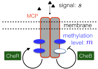
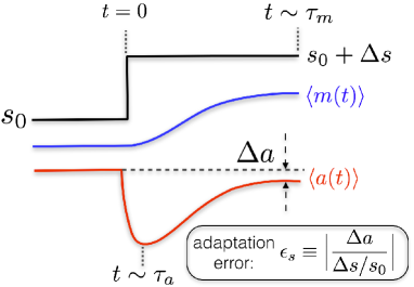
Figure 1: (a) The MCP receptor. (b) Mean response of the MCP receptor to a stepwise signal.

A Markov network model with internal states specified by $(a,m)$ was proposed for a single MCP by Lan et al. [19], as shown in Figure 2. Transition between active and inactive states at a given methylation level takes place on the time scale $\tau_{a}$, with rates given by

$$\omega_{1}(m,s)=\frac{1}{\tau_{a}}\exp\Bigl{(}\frac{\beta}{2}\Delta E(m,s)\Bigr{)},\qquad\omega_{0}(m,s)=\frac{1}{\tau_{a}}\exp\Bigl{(}-\frac{\beta}{2}\Delta E(m,s)\Bigr{)},$$

where $\beta=1/T$ is the inverse temperature, and

$$\Delta E(m,s)=e_{0}(m_{1}-m)+f(s)$$

the free energy difference between states $(0,m)$ and $(1,m)$, with $f(s)=\ln[(1+s/K_{i})/(1+s/K_{a})]$. Here $e_{0}>0$ is the methylation energy, $m_{1}$ an offset methylation level [20, 1], and $K_{i}$ and $K_{a}(\gg K_{i})$ are equilibrium constants for ligand binding to the receptor in the inactive and active states, respectively. Transition between different methylation levels takes place on the time scale $\tau_{m}$, with rates indicated in Figure 2: when the receptor is inactive, the rate of methylation (assisted by enzyme CheR) is $K_{CR}$ while the rate of demethylation is $\alpha K_{CR}$; when the receptor is active, the rate of demethylation (assisted by CheB) is $K_{CB}$ while the rate of methylation is $\alpha K_{CB}$. An estimate of the typical methylation/demethylation cycle time is given by $\tau_{m}=k_{CB}^{-1}+k_{CR}^{-1}$.

The parameter $\alpha$ specifies the degree of disequilibrium in the system. When $\alpha=\alpha_{EQ}\equiv\exp(\beta e_{0}/2)$, global detailed balance condition is satisfied, in which case the Boltzmann distribution governed by a free energy function is recovered. For $\alpha<\alpha_{EQ}$, the system is driven out of equilibrium with generally different properties which we study using both analytical and numerical methods. Therefore $\alpha$ describes the strength of driving to keep the receptor to operate under out of equilibrium conditions.

In the numerical examples presented below, we adopt the parameter values as suggested in Ref. [19]: $m_{1}=1$, $K_{i}=18.2\mu$M, $K_{a}=3000\mu$M, $\beta=1$ ($kT$ as the unit of energy) and $e_{0}=2$. The time constants are chosen as $\tau_{a}=0.1s$, and $k_{CB}=k_{CR}=0.01s^{-1}$. For this parameter set, $\alpha_{EQ}=e$. To simplify the notation, we write $\omega_{1}(m,s),\omega_{0}(m,s)$ as $\omega_{1}(m)$ and $\omega_{0}(m)$ respectively.

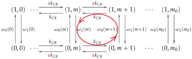
Figure 2: The Markov network model of a single receptor MCP in E. coli. Red arrows indicate existence of a futile cycle at small $\alpha$, which is essential for adaptation.

3 Adaptation and the NESS

3.1 Condition for adaptation

We first revisit the condition for adaptation first obtained by Lan et al. [19]. For the model introduced in Sec. 2, the master equation for the joint probability $P(a,m)$ takes the form,

$$\frac{dP(0,m)}{dt} = k_{CR}P(0,m-1)+\alpha k_{CR}P(0,m+1)+\omega_{1}(m)P(1,m)$$ (1a)

$$-[k_{CR}+\alpha k_{CR}+\omega_{0}(m)]P(0,m),$$

$$\frac{dP(1,m)}{dt} = \alpha k_{CB}P(1,m-1)+k_{CB}P(1,m+1)+\omega_{0}(m)P(0,m)$$ (1b)

$$-[\alpha k_{CB}+k_{CB}+\omega_{1}(m)]P(1,m).$$

From the above, we obtain the evolution equations for the moments $\langle m\rangle=\sum_{a,m}mP(a,m)$ and $\langle a\rangle=\sum_{m}P(1,m)$:

$$\frac{d\langle a\rangle}{dt} = \sum_{m}\Big{[}\omega_{0}(m)P(0,m)-\omega_{1}(m)P(1,m)\Big{]},$$ (1ba)

$$\frac{d\langle m\rangle}{dt} = (1-\alpha)(k_{CR}+k_{CB})\Bigl{(}-\langle a\rangle+\frac{k_{CR}}{k_{CR}+k_{CB}}\Bigr{)}+B_{1}.$$ (1bb)

Here $B_{1}=\alpha k_{CR}P(0,0)+k_{CB}P(1,0)-k_{CR}P(0,m_{0})-\alpha k_{CB}P(1,m_{0})$ depends on the probabilities for the extreme methylation states $m=0$ and $m=m_{0}$.

In a steady environment of constant ligand concentration $s$, the system is expected to reach a steady state in a time $\tau_{m}$ where both $\langle m\rangle$ and $\langle a\rangle$ assume constant values. Setting the right-hand-side of Eq. (1bb) to zero yields,

$$\langle a\rangle=a_{s}=\frac{k_{CR}}{k_{CR}+k_{CB}}+\frac{1}{1-\alpha}\frac{B_{1}}{k_{CR}+k_{CB}}.$$ (1bc)

Since the methylation and demethylation rates $k_{CR}$ and $k_{CB}$ are assumed to be constants in the model, the first term $a_{0}\equiv k_{CR}/(k_{CR}+k_{CB})$ on the right-hand-side of Eq. (1bc) is independent of $s$. Figure 3 shows $a_{s}$ against $s$ for three different values of $\alpha$, obtained from numerically exact solution of the model in the NESS. The steady-state activity $a_{s}$ is centered around $a_{0}$ (dashed line) over a large range of $s$ for $\alpha<1$, but not so for $\alpha\geq 1$. The “adaptation error”

$$\epsilon\equiv|a_{s}-a_{0}|=\Big{|}\frac{1}{1-\alpha}\frac{B_{1}}{k_{CR}+k_{CB}}\Big{|}$$ (1bd)

is essentially controlled by the size of the boundary term $B_{1}$. For $\alpha<1$, $B_{1}$ is small over a broad range of $s$. As we shall see in the next section, the NESS distribution in this case is indeed centered in the middle of the allowed methylation range. This is however not the case when $\alpha>1$.

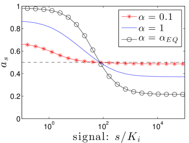
Figure 3: Mean receptor activity against ligand concentration for three different values of the nonequilibrium parameter $\alpha$. The dash line indicates the value $a_{0}$. Here the methylation range $m_{0}=4$.

The transient response to a signal ramp also exhibits qualitatively different behavior for $\alpha<1$ and $\alpha>1$. Figure 4 shows our results obtained by numerically integrating the master equations (1a) and (1b) at three different values of $\alpha$, upon a jump in ligand concentration from $10K_{i}$ to $15K_{i}$ at $t=0$. The initial response of $\langle a\rangle$ to the signal ramp is qualitatively similar in the three cases, i.e., a fast depression of receptor activity to a near plateau value in a time of order $\tau_{a}$. However, opposite behavior is seen at longer times, in concert with the change in methylation level as seen in Fig.  4(b). For $\alpha>1$, a further decrease of the mean activity is seen when the methylation level starts to decrease in response to the change in $\langle a\rangle$. On the other hand, when $\alpha<1$, the methylation level increases in accordance with Eq. (1bb), eventually restoring the mean activity to a value close to the pre-stimulus level. The latter is precisely the scenario for adaptation that employs a change in the methylation level to offset the activity change effected by the shift in signal strength.

In summary, both the steady-state activity and the transient response to a signal ramp show qualitatively different behavior below and above $\alpha=1$. We thus conclude that the condition for adaptation in this model is $\alpha<1$.

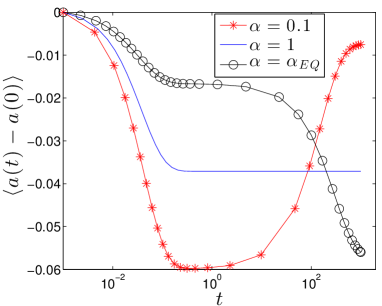
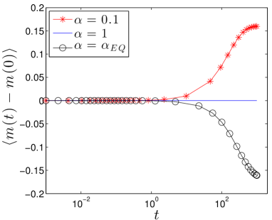
Figure 4: An initial steady state at $s=10K_{i}$ is perturbed by shifting the ligand concentration to $s=15K_{i}$ at $t=0$. Results at three different values of $\alpha$ are shown: (a) change in the mean receptor activity $\langle a(t)\rangle$ against $t$; (b) change in the methylation level $\langle m(t)\rangle$ against $t$. The methylation range $m_{0}$ is set to be four.

3.2 The NESS distribution

In the previous subsection, we obtained the condition for adaptation by considering the moment equations with the help of numerical integration of the master equation. To gain a complete understanding of the NESS, it is necessary to calculate the distribution function $P(a,m)$. Fortunately, for the model in question, this can be done under the “fast equilibrium” approximation facilitated by the separation of the time scales $\tau_{a}$ and $\tau_{m}\gg\tau_{a}$. Then, $P(1,m)$ and $P(0,m)$ satisfy the local detailed balance

$$\frac{P(1,m)}{P(0,m)}=\frac{\omega_{0}(m)}{\omega_{1}(m)}+O(\tau_{a}/\tau_{m}),\qquad(0\leq m\leq m_{0}).$$ (1be)

Let $P(m)\equiv P(0,m)+P(1,m)$, we obtain,

$$P(0,m)=\frac{1}{1+\exp[-\beta\Delta E(m,s)]}P(m),\qquad P(1,m)=\frac{\exp[-\beta\Delta E(m,s)]}{1+\exp[-\beta\Delta E(m,s)]}P(m).$$ (1bf)

With the help of (1be), Eqs. (1a) and (1b) combine to yield

$$\frac{dP(m)}{dt}=b(m-1)P(m-1)+d(m+1)P(m+1)-[b(m)+d(m)]P(m).$$ (1bg)

Equation (1bg) defines a one-dimensional birth-death process with the birth and death rates given respectively by,

$$b(m)=\frac{k_{CR}+\alpha k_{CB}\exp[-\beta\Delta E(s,m)]}{1+\exp[-\beta\Delta E(s,m)]},\qquad d(m)=\frac{\alpha k_{CR}+k_{CB}\exp[-\beta\Delta E(s,m)]}{1+\exp[-\beta\Delta E(s,m)]}.$$

Its steady-state distribution takes the form,

$$P(m+1)=\frac{b(m)}{d(m+1)}P(m)=P(0)\prod_{i=0}^{m}\frac{b(i)}{d(i+1)}.$$ (1bh)

Together with Eq. (1bf) the full NESS distribution is obtained.

Consider the range of ligand concentrations where the receptor is functional, i.e., $\exp[-\Delta E(m,s)]\ll 1$ at $m=0$ (inactive state favored) and $\exp[-\Delta E(m,s)]\gg 1$ at $m=m_{0}$ (active state favored). Consequently, the ratio $b(m)/d(m+1)$ changes monotonically between the limiting values $1/\alpha$ and $\alpha$ as $m$ increases from $0$ to $m_{0}$. Let $m^{*}$ be the value of $m$ where $b(m^{*})/d(m^{*}+1)\simeq 1$. According to Eq. (1bh), this is the methylation level where $P(m)$ varies slowest with $m$, i.e., the stationary point of the distribution. For $\alpha<1$, $b(m)/d(m+1)>1$ on the low methylation side ($m<m^{*}$) while $b(m)/d(m+1)<1$ on the high methylation side ($m>m^{*}$). Therefore $P(m)$ reaches its peak value at $m^{*}$. The opposite situation happens for $\alpha>1$, where $P(m)$ initially decreases with $m$ on the low methylation side, reaches its minimum value at $m^{*}$, and increases on the high methylation side. At $\alpha=1$, $b(m)=d(m)$ so that $P(m)=P(0)b(0)/d(m)$ becomes essentially flat especially when $k_{CR}=k_{CB}$. The general behavior of the NESS distributions in the two regimes are illustrated in Figure 5. A more complete discussion of the functional form of these distributions and their dependence on $s$ at different $\alpha$ values can be found in the Appendix A.

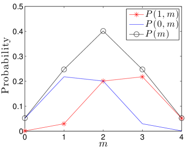
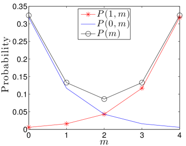
Figure 5: The steady-state distributions $P(1,m)$, $P(0,m)$ and $P(m)$ at $m_{0}=4$, $s=10K_{i}$. (a) $\alpha=0.1$; (b) $\alpha=\alpha_{EQ}>1$.

In the case $\alpha<1$, the signal level affects the shape of the distribution by shifting its peak position $m^{*}=m_{1}+f(s)/e_{0}-(\beta e_{0})^{-1}\ln(k_{CB}/k_{CR})$ (see Appendix A) which coincides with the mean methylation level. This is a general feature for adaptation achieved through integral feedback control, i.e., the effect of external signal change is absorbed by a shift in the average methylation level.

3.3 Adaptation error

According to Eq. (1bc), the mean receptor activity $\langle a\rangle$ in the NESS depends on the signal level $s$ only through the probabilities for the extreme methylation states at $m=0$ and $m=m_{0}$. For $\alpha<1$, $P(m)$ decreases rapidly away from the peak position at $m^{\ast}$. Except very close to $\alpha=1$ which requires a separate treatment, the adaptation error as defined by Eq. (1bd) can be estimated by the largest term in the expression for $B_{1}$. Let $m_{d}\equiv{\rm min}\{m^{*},m_{0}-m^{*}\}$ be the distance between $m^{\ast}$ and the closest extreme methylation state. With the help of Eq. (1bq), we obtain,

$$\ln\epsilon\simeq\left\{\begin{array}[]{lc}-{1-\alpha\over 1+\alpha}{\beta e_{0}\over 2}m_{d}^{2},&m_{d}<{\alpha+1\over\alpha-1}{1\over\beta e_{0}}\ln\alpha;\\ m_{d}\ln\alpha+{1+\alpha\over 1-\alpha}{1\over 2\beta e_{0}}\ln^{2}\alpha,&{\rm otherwise.}\end{array}\right.$$ (1bi)

Equation (1bi) shows that the adaptation error can be decreased by either increasing the methylation range $m_{0}$ or decreasing the parameter $\alpha$ that brings the system further away from equilibrium. At a given $\alpha<1$, increasing $m_{0}$ allows a greater functional range of the receptor and consequently larger values for $m_{d}$, resulting in an exponential decrease of $\epsilon$. On the other hand, at a fixed $m_{0}$, decreasing $\alpha$ increases the rate of exponential decay of $\epsilon$. However, when $\alpha$ is below $\alpha_{m}=\exp(-\beta e_{0}m_{0}/2)$, the error basically saturates to a value bounded from below by $\epsilon_{m}\simeq\exp(-\beta e_{0}m_{0}^{2}/8)$. These observations are in agreement with the trends see in Fig. 6(a) where $\epsilon$ is plotted against $\alpha$ for several different values of $m_{d}$.

4 Energy dissipation and the ESA trade-off

The nonequilibrium methylation/demethylation dynamics of the MCP receptor requires energy input [19]. Within the adaptation model considered here, the rate of energy dissipation can be calculated using the standard formula [21, 22, 23]

$$\dot{W}=\frac{1}{2\beta}\sum_{X,X^{\prime}}J(X|X^{\prime})\ln\frac{\omega(X|X^{\prime})}{\omega(X^{\prime}|X)}.$$ (1bj)

Here $\omega(X|X^{\prime})$ is the transition rate from state $X^{\prime}$ to state $X$, $J(X|X^{\prime})=\omega(X|X^{\prime})P(X^{\prime})-\omega(X^{\prime}|X)P(X)$ is the net flux from $X^{\prime}$ to $X$, and $P(X)$ is the probability for state $X$. For our purpose, it is convenient to rewrite the above equation in terms contributions from directed “elementary cycles”  [24]. An elementary cycle is a loop formed by nodes and edges of the network that cannot be further decomposed into smaller loops. Denoting by $C_{l}$ the $l$th elementary cycle on the network, Eq. (1bj) can be rewritten as

$$\dot{W}=\frac{1}{\beta}\sum_{l}J(C_{l})\mathcal{A}(C_{l}),$$ (1bk)

where $J(C_{l})$ is the probability flux associated with cycle $C_{l}$, and $\mathcal{A}(C_{l})=\sum_{e\in C_{l}}\ln[\omega(X^{\prime}|X)/\omega(X|X^{\prime})]$, summed along the cycle.

For the network model shown in Fig. 2, we define the $m$th elementary cycle to be the rectangle between methylation levels $m$ and $m+1$, directed counter-clockwise as indicated by the red arrows. It is simple to verify that the thermodynamic force $\mathcal{A}(C_{l})=2\ln[\alpha_{EQ}/\alpha]$ is the same for all cycles. The cycle flux $J(m)=k_{CB}P(1,m+1)-\alpha k_{CB}P(1,m)$ can also be read off easily from the figure. From Eq. (1bk) we then obtain,

$$\dot{W} = {2\over\beta}\Bigl{(}\ln\frac{\alpha_{EQ}}{\alpha}\Bigr{)}\sum_{m=0}^{m_{0}-1}[k_{CB}P(1,m+1)-\alpha k_{CB}P(1,m)]$$

$$= {2k_{CB}\over\beta}\Bigl{(}\ln\frac{\alpha_{EQ}}{\alpha}\Bigr{)}[(1-\alpha)a_{s}-P(1,0)+\alpha P(1,m_{0})].$$

With the help of Eq. (1bc), we obtain finally the following exact expression for the energy dissipation in the NESS,

$$\dot{W}=\frac{2}{\beta\tau_{m}}\Big{(}1-\alpha+B_{2}\Big{)}\ln\frac{\alpha_{EQ}}{\alpha},$$ (1bl)

where $B_{2}=\alpha P(0,0)-P(1,0)+\alpha P(1,m_{0})-P(0,m_{0})$ is a boundary term.

Figure 6(b) shows $\dot{W}$ against $\alpha$ for selected values of $m_{d}$. In all cases presented, a logarithmic increase on the far-from-equilibrium side (i.e., $\alpha\ll 1$) is seen, in agreement with Eq. (1bl). Dependence of $\dot{W}$ on $m_{d}$, which enters only through the boundary term $B_{2}$, is essentially negligible. This behavior can be understood from the fact that most of the dissipation takes place in the loop centered around the peak position $m^{\ast}$ of the NESS distribution $P(m)$.

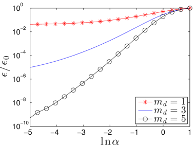
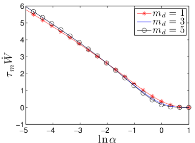
Figure 6: (a) Adaptation error and (b) energy dissipation over the methylation time scale $\tau_{m}$ against $\ln\alpha$. Here the ligand concentration is chosen such that $m_{d}=m^{*}=m_{0}/2-1$ with $m_{0}=4,\;8$ and $12$.

In Ref. [19], based on approximate solutions of the adaptation model at $m_{0}=4$, Lan et al. proposed the Energy-Speed-Accuracy tradeoff relation,

$$\dot{W}\simeq(c_{0}\sigma_{a}^{2})\omega_{m}\ln(\epsilon_{0}/\epsilon)$$ (1bm)

to capture the increase in energy dissipation to achieve higher accuracy of adaptation as $\alpha$ is reduced. Here $c_{0}\sigma_{a}^{2}$ sets the appropriate energy scale for the problem, and $\omega_{m}=\tau_{m}^{-1}$. Comparing with our results Eqs. (1bi) and (1bl), we see that Eq. (1bm) needs to be modified to take into account the dependence of $\epsilon$ on the distance $m_{d}$ from the actual mean methylation level to the boundaries of the full methylation range, i.e., $m=0$ and $m=m_{0}$. In addition, as we see from Fig. 6 , the adaptation error saturates to a value of the order of $\epsilon_{m}$ set by $m_{0}$ when $\alpha$ falls below $\alpha_{m}$, while the energy dissipation rate $\dot{W}$ keeps increasing. From the calculations presented above, we see that $\epsilon$ is controlled by the probabilities for the rare events where the extreme methylation states are visited, while $\dot{W}$ is not sensitive to the actual methylation level itself.

5 Phase transition

As we have seen in Sec. 3, there is a qualitative change in the shape of the NESS distribution $P(m)$ at $\alpha=1$. For $\alpha>1$, $P(m)$ is bimodal with peaks at the two ends of the methylation range from $0$ to $m_{0}$. The relative weight of the peaks is controlled by the signal strength $s$. On the other hand, for $\alpha<1$, $P(m)$ has a single peak in the middle of the methylation range. As the signal strength $s$ varies, the peak position shifts accordingly but its shape remains more or less the same until either end of the methylation range is reached. As discussed previously by Lan et al. [19], the latter feature is crucial for the implementation of precise adaptation. In this section we examine the transition between the two regimes in further detail with the help of the exact solution for the NESS.

Let us first examine the behavior of the energy dissipation rate in the NESS given by Eq. (1bl) in the limit $m_{d}=\min\{m^{\ast},m_{0}-m^{\ast}\}\rightarrow\infty$. For $\alpha<1$, Eq. (1bq) shows that the boundary probabilities vanish in this limit, and hence $B_{2}=0$. On the other hand, for $\alpha>1$, this limit implies the activation energies $\Delta E(0,s)\rightarrow+\infty$ and $\Delta E(m_{0},s)\rightarrow-\infty$. Therefore the receptor is nearly exclusively in the inactive state when the methylation level is close to zero, and exclusively in the active state when the methylation level is close to full. Then, the elementary loop current $J(m)=0$ for all $m$ which in turn yields vanishing dissipation. Here we encounter an interesting example where the detailed balance is violated by the kinetic rates but no dissipation actually takes place due to vanishing loop currents. Summarizing, we have in the limit $m_{d}\rightarrow\infty$,

$$\dot{W}_{\infty}=\left\{\begin{array}[]{cc}{2\over\beta\tau_{m}}(1-\alpha)\ln(\alpha_{EQ}/\alpha),&0<\alpha<1;\\ 0,&1\leq\alpha\leq\alpha_{EQ}.\end{array}\right.$$ (1bn)

The singular behavior of $\dot{W}$ against $\alpha$ indicates a true nonequilibrium transition in the model where the methylation range is infinite.

According to Eq. (1bi), the adaptation error $\epsilon$ can be made arbitrarily small in the entire adaptive phase $\alpha<\alpha_{c}=1$ by increasing $m_{d}$. On the other hand, $\dot{W}$ can be made arbitrarily small at the same time by choosing an $\alpha$ close to $\alpha_{c}$. The energy dissipation is necessary to generate adaptive behavior, however, there does not appear to be a minimal value for the dissipation rate to support an arbitrarily accurate adaptive system.

For a system with a finite methylation range, transition between the two phases is more gradual than what is described above. From Eqs. (1bq) and (1br), one may identify a “correlation length” $\lambda\simeq 1/|\ln\alpha|\simeq|1-\alpha|^{-1}$. For $m_{d}>\lambda$, Eq. (1bn) can be directly applied. Corrections need to be considered when $m_{d}<\lambda$, based on exact results derived in previous sections.

6 Conclusions

In this paper, we report a detailed analytical study of the stochastic network model proposed by Lan et al. shown previously to describe well sensory adaptation in E. coli. To understand this system, we first derive moment equations which are closely related to the rate equations traditionally used to model this type of biological processes. The moment equations implement an integral feedback control scheme at the heart of the adaptive behavior. Adaptation in the model is achieved when the nonequilibrium parameter $\alpha<\alpha_{c}$, where $\alpha_{c}=1$ is less than its value $\alpha_{EQ}$ when detailed balance is observed. By mapping the original ladder network to a one-dimensional birth-death process under the assumption of timescale separation, we obtain analytic expressions for the NESS distribution with qualitatively different behavior for $\alpha>1$ (nonadaptive phase) and $\alpha<1$ (adaptive phase). With the help of the exact results on the NESS distribution, we compute the mean receptor activity from which its dependence on the external signal strength is obtained. In the adaptive phase, the adaptation error, which measures the deviation of the mean receptor activity from a suitable reference value, is found to decrease when the system is driven further out of equilibrium by reducing $\alpha$, but approaches a saturated value for $\alpha<\alpha_{m}$. Interestingly, at a given $\alpha$, the adaptation error decreases exponentially with the number of the available methylation states before the extreme methylation levels are reached.

We also derive an exact formula for the energy dissipation rate by using a cycle-decomposition technique. The energy dissipation rate is found to be insensitive to the size of the methylation range and also to timescale separation. Although our results confirm qualitatively the statement that adaptation within the molecular construct that implements integral feedback control requires nonequilibrium driving, there does not appear to be a lower bound on energy dissipation to achieve a given level of adaptation accuracy, in contrary to the Energy-Speed-Accuracy tradeoff relation proposed previously by Lan et al.

Although the methylation range of a single MCP receptor is four, we have investigated the behavior of the system with arbitrary methylation range, especially when the methylation range $m_{0}$ is large. The extension allows us to examine various theoretical issues quantitatively. In the limit $m_{0}\rightarrow\infty$, a true nonequilibrium phase transition at $\alpha=1$ can be identified.

The current analysis only focuses on the static properties of the system. However, the transient response at short times is also an important component of the molecular adaptive circuit. An understanding of the adaptive behavior in a general setting based on thermodynamic principles is still lacking. In this respect, lessons may be drawn from recent developments in information thermodynamics [18, 25, 26] by viewing the adaptive circuit as an information processing machine.

Appendix A Approximate expression of the NESS distribution

In this Appendix we derive an approximate analytic expression for the NESS distribution given by Eq. (1bh). Taking the logarithm of the equation, we obtain,

$$\ln{P(m+1)\over P(0)}=\sum_{i=0}^{m}\ln{b(i)\over d(i+1)}=\ln{d(0)\over d(m+1)}+\sum_{i=0}^{m}\phi\bigl{(}x(i)\bigr{)},$$ (1bo)

where

$$\phi(x)=\ln{1+\alpha e^{x}\over\alpha+e^{x}}$$

and $x(m)\equiv-\beta\Delta E(s,m)+\ln(k_{CB}/k_{CR})=\beta e_{0}(m-m^{*})$, with $m^{*}=m_{1}+f(s)/e_{0}-(\beta e_{0})^{-1}\ln(k_{CB}/k_{CR})$. It is straightforward to verify that $\phi(x)$ is an odd function of $x$.

The function $\phi(x)$ is well approximated by a piece-wise linear function

$$\psi(x)=\left\{\begin{array}[]{cc}-\ln\alpha,&x\leq-\xi;\\ {\alpha-1\over\alpha+1}x,&-\xi<x<\xi;\\ \ln\alpha,&x\geq\xi.\end{array}\right.$$ (1bp)

which has the same slope at $x=0$ and same asymptotic values as $x\rightarrow\pm\infty$. Continuity requires the choice $\xi={\alpha+1\over\alpha-1}\ln\alpha$. The two functions match each other well except near $x=\pm\xi$.

For $\alpha<1$, the peak of $P(m)$ is centered at $m^{\ast}$. It is thus convenient to use $P(m^{*})$ as the reference. Approximating the sum in Eq. (1bo) by an integral over $\psi(x)$, we obtain,

$$\ln{P(m)\over P(m^{*})}\simeq\left\{\begin{array}[]{ll}-(m-m^{\ast})\ln\alpha+\ln{d(m^{*})\over d(m)}+{1+\alpha\over 1-\alpha}{1\over 2\beta e_{0}}\ln^{2}\alpha,&m<m_{-};\\ -{1-\alpha\over 1+\alpha}{\beta e_{0}\over 2}(m-m^{\ast})^{2}+\ln{d(m^{*})\over d(m)},&m_{-}<m<m_{+};\\ (m-m^{\ast})\ln\alpha+\ln{d(m^{*})\over d(m)}+{1+\alpha\over 1-\alpha}{1\over 2\beta e_{0}}\ln^{2}\alpha,&m>m_{+}.\end{array}\right.$$ (1bq)

Here $m_{\pm}=m^{\ast}\pm\xi/(\beta e_{0})$. Since $d(m)$ has only a relatively weak dependence on $m$, we see that $P(m)$ is essentially gaussian within the interval $(m_{-},m_{+})$, but turns to simple exponential decay outside the interval.

For $\alpha>1$, $P(m)$ achieves its minimum value at $m^{\ast}$. In the neighborhood of the methylation boundaries, we have

$$P(m)\simeq\left\{\begin{array}[]{ll}\alpha^{-m}P(0)d(0)/d(m),&m<m_{-};\\ \alpha^{m-m_{0}}P(m_{0})d(m_{0})/d(m),&m>m_{+}.\end{array}\right.$$ (1br)

Noting that $\phi(x)$ is an odd function of $x$, we have approximately $P(m_{0})\simeq\alpha^{m_{0}-2m^{\ast}}P(0)d(0)/d(m_{0})$.

References

References

- [1] Y. Tu, Annu. Rev. Biophys. 42, 337 (2013).
- [2] H. C. Berg and E. M. Purcell, Biophys. J. 20, 193 (1977).
- [3] U. Alon, M. G. Surette, N. Barkai, and S. Leibler, Nature 397, 168 (1999).
- [4] N. Barkal and S. Leibler, Nature 387, 913 (1997).
- [5] T.-M. Yi, Y. Huang, M. I. Simon, and J. Doyle, Proc. Natl. Acad. Sci. USA 97, 4649 (2000).
- [6] W. Ma, A. Trusina, H. El-Samad, W. A. Lim, and C. Tang, Cell 138, 760 (2009).
- [7] C. Jarzynski, Phys. Rev. Lett. 78, 2690 (1997).
- [8] F. Ritort, Adv. Chem. Phys. 137, 31 (2008).
- [9] K. Sekimoto, Stochastic energetics, Lecture Notes in Physics, Berlin Springer-Verlag, Vol. 799 (2010).
- [10] T. Harada and S.-i. Sasa, Phys. Rev. E 73, 026131 (2006).
- [11] S. Toyabe, T. Okamoto, T. Watanabe-Nakayama, H. Taketani, S. Kudo, and E. Muneyuki, Phys. Rev. Lett. 104, 198103 (2010).
- [12] U. Seifert, Rep. Prog. Phys. 75, 126001 (2012).
- [13] M. Esposito, U. Harbola, and S. Mukamel, Phys. Rev. E 76, 031132 (2007).
- [14] J. J. Hopfield, Proc. Natl. Acad. Sci. USA 71, 4135 (1974).
- [15] H. Qian and T. C. Reluga, Phys. Rev. Lett. 94, 028101 (2005).
- [16] P. Mehta and D. J. Schwab, Proc. Natl. Acad. Sci. USA 109, 17978 (2012).
- [17] G. Lan and Y. Tu, J. R. Soc. Interface 10, 20130489 (2013).
- [18] P. Sartori, L. Granger, C. F. Lee, and J. M. Horowitz, PLoS Comput. Biol. 10, e1003974 (2014).
- [19] G. Lan, P. Sartori, S. Neumann, V. Sourjik, and Y. Tu, Nat. Phys. 8, 422 (2012).
- [20] M. D. Lazova, T. Ahmed, D. Bellomo, R. Stocker, and T. S. Shimizu, Proc. Natl. Acad. Sci. USA 108, 13870 (2011).
- [21] J.L. Lebowitz and H. Spohn, J. Stat. Phys. 95 333 (1999).
- [22] U. Seifert, Phys. Rev. Lett. 95 040602 (2005).
- [23] H. Qian, Annu. Rev. Phys. Chem. 58, 113 (2007).
- [24] D. Andrieux and P. Gaspard, J. Stat. Phys. 127, 107 (2007).
- [25] K. Maruyama, F. Nori, and V. Vedral, Rev. Mod. Phys. 81, 1 (2009).
- [26] J. M. Parrondo, J. M. Horowitz, and T. Sagawa, Nature Physics 11, 131 (2015).