Bubble formation in water with addition of a hydrophobic solute

Abstract

We show that phase separation can occur in a one-component liquid outside its coexistence curve (CX) with addition of a small amount of a solute. The solute concentration at the transition decreases with increasing the difference of the solvation chemical potential between liquid and gas. As a typical bubble-forming solute, we consider O₂ in ambient liquid water, which exhibits mild hydrophobicity and its critical temperature is lower than that of water. Such a solute can be expelled from the liquid to form gaseous domains while the surrounding liquid pressure is higher than the saturated vapor pressure $p_{\rm cx}$. This solute-induced bubble formation is a first-order transition in bulk and on a partially dried wall, while a gas film grows continuously on a completely dried wall. We set up a bubble free energy $\Delta G$ for bulk and surface bubbles with a small volume fraction $\phi$. It becomes a function of the bubble radius $R$ under the Laplace pressure balance. Then, for sufficiently large solute densities above a threshold, $\Delta G$ exhibits a local maximum at a critical radius and a minimum at an equilibrium radius. We also examine solute-induced nucleation taking place outside CX, where bubbles larger than the critical radius grow until attainment of equilibrium.

I Introduction

Recently, much attention has been paid to the formation of small bubbles, sometimes called nanobubbles, in water review1 ; bridging1 ; review2 . They have been observed with a dissolved gas on hydrophobic surfaces review2 ; review1 ; bridging1 ; b0 ; b00 ; b1 ; ex10 ; ex11 ; ex12 ; ex13 ; Ducker ; type and in bulk Jin ; ex1 ; ex2 ; ex3 ; ex4 ; Bunkin in ambient conditions (around $300$ K and 1 atm), where the pressure in the bulk liquid region is larger than the saturated vapor pressure $p_{\rm cx}$ or outside the coexisting curve (CX). Their typical radius $R$ is of order $10-100$ nm and their life time is very long. The interior pressure is given by $2\sigma/R\sim$30 atm for a bubble with $R=50$ nm from the Laplace law, where $\sigma$ is the surface tension equal to $72$ erg$/$cm². Strong attractive forces have also been measured between hydrophobic walls in water due to bubble bridging bridging1 ; b0 ; b00 ; b1 ; ex1 ; ex10 ; ex12 . These effects are important in various applications, but the underlying physics has not yet been well understood.

In this paper, we ascribe the origin of bubble formation to a hydrophobic interaction between water and solute Ben ; Guillot ; Paul ; Pratt ; Chandler ; Garde . In our theory, the solute-induced phase separation generally occurs in equilibrium when the solvent is in a liquid state outside CX and the solute-solvent interaction is repulsive. Most crucial in our theory is the solvation chemical potential of the solute $\mu_{\rm s}(n,T)$ depending on the solvent density $n$ and the temperature $T$. With increasing such a repulsion, its difference $\Delta\mu_{\rm s}$ between the liquid and gas phases can be considerably larger than the thermal energy $k_{B}T$ (per solute particle). In this situation, the solute molecules are repelled from the liquid to form domains of a new phase (in gas, liquid, or solid). Supposing bubbles with a small volume fraction $\phi$, we set up a free energy $\Delta G$ accounting for considerably large $\Delta\mu_{\rm s}/k_{B}T$. Then, its minimization with respect to $\phi$ and the interior solute density $n^{\prime}_{\rm I}$ yields the equilibrium conditions of bubbles in liquid (those of chemical equilibrium and pressure balance).

As a bubble-forming solute in water, we treat O₂, which is mildly hydrophobic with $\Delta\mu_{\rm s}/k_{B}T\cong 3.44$ on CX at $T=300$ K. Furthermore, the critical temperature and pressure of water and O₂ are given by $(647.3$ K, 22.12 MPa) and ($154.6$ K, $5.043$ MPa), respectively. Notice that the critical temperature of water is much higher than that of O₂ (and than those of N₂, H₂, and Ar etc) due to the hydrogen bonding in water. As a result, no gas-liquid phase transition takes place within bubbles composed mostly of O₂ in liquid water in ambient conditions. In contrast, strongly hydrophobic solutes usually form solid aggregates in liquid water except for very small solute densities Ben ; Guillot ; Paul ; Pratt ; Chandler ; Garde .

In our theory, solute-induced bubbles can appear outside CX only when the solute density exceeds a threshold density, where the threshold tends to zero as the liquid pressure approaches $p_{\rm cx}$. In particular, above the threshold density, a surface bubble (a gas film) appears on a hydrophobic wall in the temperature range $T<T_{\rm D}$ ($T>T_{\rm D}$). As is well known, this is possible only on CX without solute (in one-component fluids). Here, $T_{\rm D}$ is the drying temperature Cahn ; Bonnreview determined by the solvent-wall interaction, so it is insensitive to a small amount of solute with mild $\Delta\mu_{\rm s}$. With a solute below the threshold density, we predict only a microsopically depleted layer outside CX (as in one-component fluids). Indeed, some groups Doshi ; G1 ; G2 detected only microscopic depletion layers on a hydrophobic wall with a dissolved gas, while other groups observed surface bubbles review2 ; review1 ; bridging1 ; b0 ; b00 ; b1 ; ex10 ; ex11 ; ex12 ; ex13 ; Ducker ; type .

On the other hand, to prepare stable bulk bubbles, macroscopic gas bubbles composed of O₂ etc. have been fragmented by stirring in liquid water Bunkin ; ex2 ; ex3 ; ex4 . In such measurements, Ohgaki et al.ex2 realized bubbles with $R\sim 50$ nm in quasi-steady states, where the bubble density was $n_{\rm b}\sim 19~{}\mu$m^-3 and the bubble volume fraction was $\phi\sim 0.01$. We shall see that the nucleation barrier of creating solute-induced bulk bubbles in quiescent states is too high for nucleation experiments for a gas such as O₂ except for very high liquid pressures.

As a similar bulk phenomenon, long-lived heterogeneities have also been observed in one-phase states of aqueous mixtures with addition of a salt or a hydrophobic solute S1 ; Curr ; Okamoto . Dynamic light scattering experiments indicated that their typical size is of order $100$ nm. Theoretically, such a phase separation can occur if the solute-solvent interaction is highly preferential between the two solvent components Curr ; Okamoto .

This paper is organized as follows. In Sec.II, we will present a thermodynamic theory of bubbles induced by a small amount of solute, where the liquid pressure and the total solvent and solute numbers are fixed. In Sec.III, we will set up a bubble free energy $\Delta G$. In Sec.IV, we will examine solute-induced nucleation. In addition, in Sec.IIIC and Appendix A, we will briefly examine bubble formation at fixed chemical potentials and at fixed cell volume.

II Equilibrium bubbles with hydrophobic solute

We consider a one-component solvent, called water, in a liquid state outside the coexistence curve (CX). We then add a small amount of a neutral, hydrophobic solute (impurities). The total solvent and solute numbers are fixed at $N=V{\bar{n}}$ and $N_{\rm I}=V{\bar{n}}_{\rm I}$, respectively, with $\bar{n}$ and ${\bar{n}}_{\rm I}$ being the initial water and solute densities. Here, ${\bar{n}}$ is larger than the liquid density $n_{\rm cx}^{\ell}$ on CX before bubble formation. We keep the pressure in the liquid region at the initial value $\bar{p}$ larger than the saturated vapor (coexistence) pressure $p_{\rm cx}$ by attaching a pressure valve to the cell, as illustrated in Fig.1. We do not assume the presence of surfactants and ions (see remarks in Sec.IVA).

II.1 Solvation chemical potential and Henry’s law

We assume that the molecular volume of solute $v_{\rm I}$ is of the same order as that of solvent $v_{\rm w}$, since large hydrophobic impurities tend to form solid precipitates Paul ; Chandler ; Garde . We then consider the Helmholtz free energy density $f$ depending on the water density $n$ and the solute density $n_{\rm I}$ in the dilute limit of solute. In this paper, we neglect the solute-solute interaction to obtain

$$f(n,n_{\rm I})=f_{\rm w}(n)+k_{B}Tn_{\rm I}[\ln(n_{\rm I}v_{\rm I})-1+\nu_{\rm s}(n)],$$ (1)

where $f_{\rm w}(n)$ is the Helmholtz free energy density of pure water and $\nu_{\rm s}(n)$ is related to the solvation chemical potential $\mu_{\rm s}(n)$ in the limit of small $n_{\rm I}$ by

$$\nu_{\rm s}(n)=\mu_{\rm s}(n)/k_{B}T.$$ (2)

Hereafter, the $T$-dependence of the physical quantities will not be written explicitly.

Note that the combination $\ln[v_{\rm I}/\lambda_{\rm I}^{3}]+\nu_{\rm s}$ can be determined unambiguously in thermodynamics in the limit $n_{\rm I}\to 0$, where $\lambda_{\rm I}$ is the thermal de Broglie length ($\propto T^{-1/2}$). Thus, $v_{\rm I}$ may be chosen to be independent of $n$ without loss of generality. It is known that the entropic contribution to $\nu_{\rm s}$ is crucial for nonpolar impurities in liquid water Pratt ; Paul ; Chandler .

From eq.(1) we calculate the chemical potential of water $\mu$ and that of solute $\mu_{\rm I}$ as

$$\mu=\partial f_{\rm w}/\partial n+k_{B}Tn_{\rm I}g_{s}(n),$$ (3)

$$\mu_{\rm I}=k_{B}T[\ln(n_{\rm I}v_{\rm I})+\nu_{\rm s}(n)],$$ (4)

where we define

$$g_{s}(n)=\frac{\partial\nu_{\rm s}}{\partial n}=\frac{1}{k_{B}T}\frac{\partial\mu_{\rm I}}{\partial n}.$$ (5)

The pressure $p=n\mu+n_{\rm I}\mu_{\rm I}-f$ is written as

$$p=[n\partial f_{\rm w}/\partial n-f_{\rm w}]+k_{B}Tn_{\rm I}[1+ng_{s}(n)],$$ (6)

where the first term is the contribution from the solvent and the second term from the solute. The typical size of $g_{s}(n)$ is of the order of the solute molecular volume $v_{\rm I}$. In the presence of bubbles, $\mu$ and $\mu_{\rm I}$ take common values in gas and liquid, while the pressure in the bubbles is higher than that in the liquid by $2\sigma/R$.

First, the homogeneity of $\mu_{\rm I}$ in equilibrium yields

$$n_{\rm I}=n_{\rm I}^{0}\exp[-{\nu}_{s}(n)],$$ (7)

as a function of $n$ in two-phase states, where $n_{\rm I}^{0}=\exp(\mu_{\rm I}/k_{B}T)/v_{\rm I}$ is a constant. In gas-liquid coexistence, let the water and solute densities be $n^{\prime}$ and $n_{\rm I}^{\prime}$ in gas and be $\hat{n}$ and ${\hat{n}}_{\rm I}$ in liquid, respectively. Then, eq. (7) gives

$${{\hat{n}}_{\rm I}}/n_{\rm I}^{\prime}=\exp[-\Delta{\nu}_{s}],$$ (8)

where the $\Delta\nu_{\rm s}={\nu}_{s}({\hat{n}})-{\nu}_{s}({n^{\prime}})$. This density ratio is called the Ostwald coefficient, which represents solubility of a gas Ben ; Guillot ; Pratt . It is much smaller than unity for large $\Delta\nu_{\rm s}$. Near CX, we may approximate $\Delta\nu_{\rm s}$ by its value on CX expressed as

$$\Delta\nu_{\rm s}=\nu_{\rm s}(n_{\rm cx}^{\ell})-\nu_{\rm s}(n_{\rm cx}^{g}),$$ (9)

where ${n}_{\rm cx}^{\ell}$ and ${n}_{\rm cx}^{g}$ are the liquid and gas densities on CX of pure water.

It is worth noting that $\Delta\nu_{\rm s}$ in eq.(9) is related to the Henry constant $k_{\rm H}$Sander ; Smith . From partitioning of a solute between coexisting gas and liquid, it is defined by

$$k_{\rm H}=k_{B}Tn^{\prime}_{\rm I}/\hat{x}=k_{B}Tn_{\rm cx}^{\ell}\exp({\Delta\nu_{\rm s}}),$$ (10)

where $k_{B}Tn^{\prime}_{\rm I}$ is the solute partial pressure in gas and $\hat{x}=\hat{n}_{\rm I}/n_{\rm cx}^{\ell}$ is the solute molar fraction in liquid. In water in the ambient conditions, $\Delta\nu_{\rm s}$ is $3.44$ for O₂, $4.12$ for N₂, and 0.18 for CO₂, where CO₂ is highly soluble in liquid water. Thus, our theory is not applicable to CO₂.

However, there are a variety of solutes with stronger hydrophobicitySander . For example, $\Delta\nu_{\rm s}=10.2$ for pentacosane. In addition, from numerical simulations, a neutral hard-sphere particle deforms the surrounding hydrogen bonding; as a result, $\Delta\nu_{\rm s}\propto a^{3}$ for $a\lesssim 1$ nm and $\Delta\nu_{\rm s}\sim 4\pi\sigma a^{2}/k_{B}T$ for $a>1$ nm with varying the particle radius $a$ Paul ; Garde ; Chandler ; Pratt . This gives $\Delta\nu_{\rm s}\sim 180$ for $a\sim 1$ nm. As hydrophobic assembly, such strongly hydrophobic solutes aggregate in liquid water.

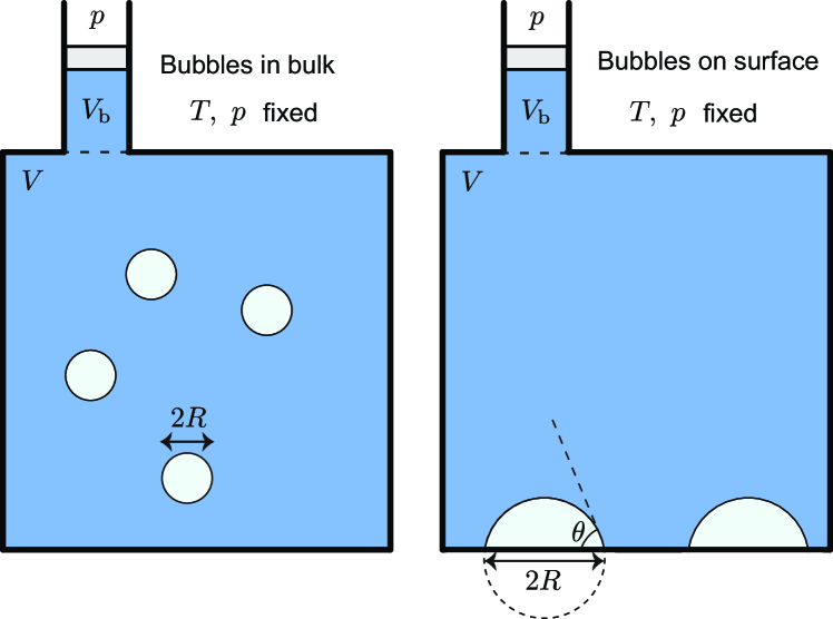
Figure 1: (Color online) Illustration of experimental setup with a pressure valve realizing a constant liquid pressure $\bar{p}$ (outside bubbles) larger than $p_{\rm cx}$, where the total solvent and solute numbers are fixed. The cell contains bubbles in bulk (left) or those on a wall (right). The volume of the cell is $V$ and that of the valve region is $V_{b}$, where $V_{b}$ is nearly equal to $\phi V$ for small bubble volume fraction $\phi$ in the cell.

II.2 Chemical equilibrim and pressure balance

We consider bubbles in bulk or on a wall at a small volume fraction $\phi$ in the cell. For simplicity, we assume no bubble in the valve region in Fig.1. If the water density inside the bubbles $n^{\prime}$ is much smaller than $\bar{n}$, the valve volume $V_{b}$ is given by

$$V_{b}=V\phi.$$ (11)

Since the total solvent and solute numbers are fixed, the densities in the liquid are given by

$$\hat{n}=\bar{n}-\phi n^{\prime}\cong{\bar{n}},$$ (12)

$${\hat{n}}_{\rm I}={\bar{n}}_{\rm I}-\phi{n}_{\rm I}^{\prime}$$ (13)

Hereafter, we set ${\hat{n}}={\bar{n}}$. We also have $\phi<{\bar{n}}_{\rm I}/n_{\rm I}^{\prime}\ll 1$ from ${\hat{n}}_{\rm I}>0$. Thus, the chemical equilibrium condition (8) and the conservation relation (13) give

$$n_{\rm I}^{\prime}={\bar{n}}_{\rm I}/[\phi+\exp(-{\Delta\nu}_{s})],$$ (14)

$${\hat{n}}_{\rm I}={\bar{n}}_{\rm I}/[1+\phi\exp({\Delta\nu}_{s})].$$ (15)

The fraction of the solute in the bubbles is given by

$$\alpha=\phi n_{\rm I}^{\prime}/{\bar{n}}_{\rm I}=\phi/[\phi+\exp(-{\Delta\nu}_{s})],$$ (16)

which tends to 1 for $\phi\gg\exp(-{\Delta\nu}_{s})$.

We write the value of the water chemical potential $\mu$ in eq.(3) in the gas as $\mu^{\prime}$ and that in the liquid as $\hat{\mu}$, where $\mu^{\prime}=\hat{\mu}$ in equilibrium. Since ${\bar{p}}$ is close to $p_{\rm cx}$, it is convenient to measure them from the chemical potential $\mu_{\rm cx}$ on CX for pure water. Here, $n^{\prime}$ is small in the gas and use can be made of the Gibbs-Duhem relation in the liquid. Then, we obtain

$$\mu^{\prime} = \mu_{\rm cx}+k_{B}T[\ln(n^{\prime}/n_{\rm cx}^{g})+n_{\rm I}^{\prime}g_{s}(n^{\prime})],$$ (17)

$$\hat{\mu} = {\bar{\mu}}=\mu_{\rm cx}+({\bar{p}}-p_{\rm cx})/n_{\rm cx}^{\ell},$$ (18)

where $\hat{\mu}$ remains equal to the initial value $\bar{\mu}$. To linear order in the deviation $n^{\prime}-n_{\rm cx}^{g}$ in eq.(17), the chemical equilibrium condition $\mu^{\prime}=\hat{\mu}$ yields

$$n^{\prime}/n_{\rm cx}^{g}-1=({\bar{p}}-p_{\rm cx})/k_{B}Tn_{\rm cx}^{\ell}-n_{\rm I}^{\prime}g_{s}(n^{\prime}),$$ (19)

In the right hand side of eq.(19), we may neglect the first term for $\hat{p}-p_{\rm cx}\ll k_{B}Tn_{\rm cx}^{\ell}$ and the second term for $n_{\rm I}^{\prime}v_{\rm I}\ll 1$ (see the sentence below eq.(6)). Then, we find

$$n^{\prime}=n_{\rm cx}^{g}=p_{\rm cx}/k_{B}T.$$ (20)

For one-component fluidsKatz , the pressure in a bubble has been set equal to $p_{\rm cx}$ from $n_{\rm cx}^{g}/n_{\rm cx}^{\ell}\ll 1$ far from the critical point. In the present mixture case, the gas pressure is $p^{\prime}=k_{B}Tn_{\rm I}^{\prime}+p_{\rm cx}$. With the aid of the Laplace law $p^{\prime}={\bar{p}}+2\sigma/R$, we obtain the pressure balance equation,

$$k_{B}Tn^{\prime}_{\rm I}={\bar{p}}-p_{\rm cx}+2\sigma/R.$$ (21)

Eliminating $n_{\rm I}^{\prime}$ from eqs.(14) and (21), we may express the volume fraction $\phi$ as

$$\phi=k_{B}T{\bar{n}}_{\rm I}/({\bar{p}}-p_{\rm cx}+2\sigma/R)-e^{-{\Delta\nu}_{s}}.$$ (22)

From eqs.(20) and (21), we find $n^{\prime}_{\rm I}\gg n^{\prime}$ for ${\bar{p}}-p_{\rm cx}\gg p_{\rm cx}$ or for $R\ll 2\sigma/p_{\rm cx}$, where the gas consists mostly of the solute. For water at $T=300$ K, we have $p_{\rm cx}=3.6$ kPa and $n_{\rm cx}^{g}=0.86\times 10^{18}/$cm³, where $n_{\rm I}^{\prime}\gg n^{\prime}$ holds for ${\bar{p}}\gg 0.0036$ atm or for $R<40~{}\mu$m. In addition, at ${\bar{p}}=1$ atm, we have $n^{\prime}_{\rm I}\cong 2\sigma/k_{B}TR$ for $R\ll 1.4$ $\mu$m.

In the limit of $\phi\to 0$ and $R\to\infty$, eq.(22) gives a threshold solute density for gas film formation,

$$n_{\rm I}^{c}=e^{-\Delta{\nu}_{s}}({\bar{p}}-p_{\rm cx})/k_{B}T,$$ (23)

which vanishes as ${\bar{p}}\to p_{\rm cx}$ and is small for large $\Delta{\nu}_{s}$. Here, we introduce the following parameter,

$$\gamma={\bar{n}}_{\rm I}/n_{\rm I}^{c}-1.$$ (24)

A gas film can appear for $\gamma>0$, but bubbles with $R^{-1}>0$ can be stable for $\gamma>\gamma_{\rm tr}$ with $\gamma_{\rm tr}$ being a positive threshold (see Fig.4). For O₂ in water at $T=300$ K, we have $n_{\rm I}^{c}=0.78\times 10^{18}({\bar{p}}-p_{\rm cx})$ cm^-3 with pressures in atm. The corresponding oxygen mole fraction is $2.3\times 10^{-5}({\bar{p}}-p_{\rm cx})$.

II.3 Gas film at fixed pressure

We consider a gas film on a hydrophobic wall, where there is no contact between the wall and the liquid phase Setting $R^{-1}=0$ in eq.(22), we obtain $\phi$ for $\gamma>0$ as

$$\phi = ({\bar{n}}_{\rm I}-n^{c}_{\rm I})k_{B}T/({\bar{p}}-p_{\rm cx})$$ (25)

$$= \gamma\exp(-\Delta{\nu}_{s}).$$

In this case, we have ${\hat{n}}_{\rm I}={\bar{n}}_{\rm I}/(1+\gamma)$ from eq.(15). For $\gamma<0$, water is only microscopically depleted at the wall, though the depletion layer itself can be influenced by the soluteDoshi . In the present isobaric case, $\phi$ increases and even approaches unity as ${\bar{p}}-p_{\rm cx}\to 0$, so we need to require ${\bar{p}}-p_{\rm cx}>k_{B}T({\bar{n}}_{\rm I}-n^{c}_{\rm I})$. In contrast, at fixed cell volume, $\phi$ remains small even for ${\bar{p}}-p_{\rm cx}\leq 0$ (see Appendix A).

II.4 Bubbles with a common radius at fixed pressure

We suppose bubbles with a common curvature $R^{-1}$ outside CX. Using the relation $k_{B}T{\bar{n}}_{\rm I}/({{\bar{p}}-p_{\rm cx}})=(\gamma+1)\exp(-\Delta\nu_{\rm s})$, we rewrite eq.(22) as

$$\phi=\frac{k_{B}T({\bar{n}}_{\rm I}-n_{\rm I}^{c})}{{\bar{p}}-p_{\rm cx}}\cdot\frac{R-R_{c}}{R+\gamma R_{c}},$$ (26)

which tends to eq.(25) in the limit $R\to\infty$. Here, we introduce the critical radius $R_{c}$ defined by

$$R_{c}=2\sigma/\gamma({{\bar{p}}-p_{\rm cx}}).$$ (27)

Here, $R_{c}=1.4/\gamma$ $\mu$m for ambient water ($300$ K and $1$ atm). We need to require $R>R_{c}$ outside CX since $\phi>0$. See $R_{c}$ for O₂ in water in Fig.5(a). For bubble nucleation in one-component fluidsKatz ; Caupin ; Onukibook , the critical radius is given by $R_{c}=2\sigma/(p_{\rm cx}-{\bar{p}})$ with ${\bar{p}}<p_{\rm cx}$.

We assume $N_{\rm b}$ bubbles in the cell neglecting bubble coalescence. Then, we express $\phi$ as

$$\phi=4\pi R^{3}G(\theta)n_{\rm b}/3,$$ (28)

where $n_{\rm b}=N_{\rm b}/V$ is the bubble density. For bulk bubbles we set $G(\theta)=1$. For surface bubbles it is given by Turnbull’s formula hetero ; Binder ,

$$G(\theta)=(2-3\cos\theta+\cos^{3}\theta)/4,$$ (29)

where $\theta$ is the (gas-side) contact angle in the partial drying condition determined by Young’s relation,

$$\cos\theta=(\sigma_{\rm w}^{\ell}-\sigma_{\rm w}^{g})/\sigma.$$ (30)

where $\sigma_{\rm w}^{\ell}$ and $\sigma_{\rm w}^{g}$ are the free energies per area between the wall and the liquid and gas phases, respectively, and we assume $|\sigma_{\rm w}^{\ell}-\sigma_{\rm w}^{g}|<\sigma$. Here, $0\leq\theta<\pi/2$ for a hydrophobic wall and $\pi/2<\theta\leq\pi$ for a hydrophilic wall. As $\theta\to 0$, we have the complete drying condition $\sigma_{\rm w}^{\ell}-\sigma_{\rm w}^{g}=\sigma$ at $T=T_{\rm D}$ on CX. As $\theta\to\pi$, the bubbles tend to be detached from the wall, resulting in bulk bubbles. Experimentally, $\theta$ for surface bubbles has been observed in a range of $10$-$30^{\circ}$review2 . Note that eqs.(26) and (28) constitute a closed set of equations determining the equilibrium radius $R$ for each given ${\bar{n}}_{\rm I}$, $\theta$, and $n_{\rm b}$.

III Bubble free energy

III.1 Derivation using grand potential density

In the geometry in Fig.1 with a pressure valve, we should derive the equilibrium conditions of bubbles from minimization of the Gibbs free energy written as

$$G = F+\sigma S+(V+V_{b}){\bar{p}}$$ (31)

$$= {\bar{G}}+\Delta G,$$

where $F$ is the Helmholtz free energy (excluding the surface contribution here) and $S$ is the total interface area. For a small volume change $V_{b}\to V_{b}+dV_{b}$, the work exerted by the fluid to the valve is ${\bar{p}}dV_{b}$ at fixed pressure, so we should consider $G$ in eq.(31). The second line is the definition of the bubble free energy $\Delta G$ with ${\bar{G}}=Vf({\bar{n}},\bar{n}_{\rm I})+V{\bar{p}}$ being the initial Gibbs free energy.

In terms of the Helmholtz free energy densities $f^{\prime}$ in the gas and $\hat{f}$ in the liquid, we have $F=V(\phi f^{\prime}+\hat{f})$ for the total system including the valve region. Here, it is convenient to introduce the grand potential density,

$$\omega(n,n_{\rm I})=f-\bar{\mu}n-\bar{\mu}_{\rm I}n_{\rm I}+{\bar{p}},$$ (32)

where $\bar{\mu}$ and $\bar{\mu}_{\rm I}$ are the initial chemical potentials for water and solute, respectively. Using eqs.(12) and (13) we obtain

$${F}/{V}=\phi\omega^{\prime}+\hat{\omega}-\phi{\bar{p}}+{\bar{f}},$$ (33)

where $\omega^{\prime}$ is the value of $\omega$ in the gas, ${\hat{\omega}}$ is that in the liquid, and $\bar{f}$ is the initial Helmholtz free energy density. Thus, eq.(31) gives

$$\Delta G=V[\phi\omega^{\prime}+\hat{\omega}]+\sigma S.$$ (34)

We note that $\omega({n},{n}_{\rm I})$ vanishes in the initial state and is second order with respect to the deviations $n-{\bar{n}}$ and $n_{\rm I}-{\bar{n}}_{\rm I}$ (see eqs.(12) and (13)). In the following we assume that the bubbles have a common curvature $R^{-1}$, where in terms of $G(\theta)$ in eq.(29) $S$ is given by hetero ; Binder ,

$$S=4\pi R^{2}G(\theta)n_{\rm b}V.$$ (35)

We next calculate $\omega^{\prime}$ and $\hat{\omega}$ for small ${\bar{p}}-p_{\rm cx}$ assuming eqs.(14) and (20). In the gas, we use $\omega^{\prime}=(\mu^{\prime}-{\bar{\mu}})n^{\prime}+(\mu_{\rm I}^{\prime}-{\bar{\mu}}_{\rm I})n_{\rm I}^{\prime}+{\bar{p}}-p^{\prime}$, where the first term in the right hand side is negligible from eq.(18). Further we set $p^{\prime}=p_{\rm cx}+k_{B}Tn_{\rm I}^{\prime}$ from eq.(20)and use eq.(3) to find

$$\omega^{\prime}=k_{B}Tn_{\rm I}^{\prime}[\ln({n_{\rm I}^{\prime}/{\bar{n}}_{\rm I}})-1-{\Delta{\nu}_{s}}]+{\bar{p}}-p_{\rm cx}.$$ (36)

In the liquid, ${\hat{n}}_{\rm I}$ is very small and we obtain

$$\hat{\omega}=k_{B}T[{\hat{n}}_{\rm I}\ln({\hat{n}}_{\rm I}/{{\bar{n}}_{\rm I}})+\phi n_{\rm I}^{\prime}],$$ (37)

where ${\hat{n}}_{\rm I}={{\bar{n}}_{\rm I}}-\phi{n}_{\rm I}^{\prime}$ from eq.(13). Thus, if $\phi\ll{\bar{n}}_{\rm I}/n_{\rm I}^{\prime}\ll 1$, the logarithm $\ln({\hat{n}}_{\rm I}/{{\bar{n}}_{\rm I}})$ can be expanded with respect to $\phi$, leading to $\hat{\omega}\propto\phi^{2}$. However, we are also interested in the case $\phi\sim{\bar{n}}_{\rm I}/n_{\rm I}^{\prime}$.

In equilibrium, $\Delta G$ in eq.(34) is minimized with respect to $n_{\rm I}^{\prime}$ and $\phi$, where $R$ and $S$ are functions of $\phi$ at fixed $\theta$ and $n_{\rm b}$. Thus, let us change $n_{\rm I}^{\prime}$ and $\phi$ infinitesimally by $\delta n_{\rm I}^{\prime}$ and $\delta\phi$, respectively. From eqs.(34)-(37), we calculate the incremental change of $\Delta G$ as

$$\delta(\Delta G) = Vk_{B}T[\ln(n_{\rm I}^{\prime}/\hat{n}_{\rm I})-\Delta\nu_{\rm s}](n_{\rm I}^{\prime}\delta\phi+\phi\delta n_{\rm I}^{\prime})$$ (38)

$$+V[{\bar{p}}-p_{\rm cx}+2\sigma/R-k_{B}Tn^{\prime}_{\rm I}]\delta\phi.$$

Therefore, the equilibrium conditions (14) and (21) follow from $\partial(\Delta G)/\partial n_{\rm I}^{\prime}=\partial(\Delta G)/\partial\phi=0$.

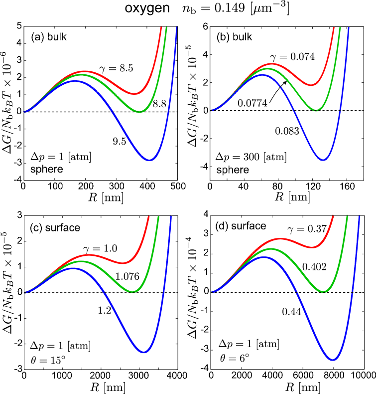
Figure 2: (Color online) Normalized bubble free energy $\Delta G/N_{\rm b}k_{B}T$ vs $R$ for O₂ in liquid water in the isobaric condition for bulk bubbles in (a) and (b) and for surface bubbles in (c) and (d), where $T=300$ K and $n_{\rm b}=N_{\rm b}/V=0.149/$$\mu$m³. The pressure difference $\Delta p={\bar{p}}-p_{\rm cx}$ is 1 atm in (a), (c), and (d) and is 300 atm in (b). The contact angle $\theta$ is $15^{\circ}$ in (c) and is $6^{\circ}$ in (d). Then, ($A,\gamma_{\rm m})=$ $(3.86,7.74)$ in (a), $(0.0129,0.0680)$ in (b), $(0.367,0.945)$ in (c), and $(0.109,0.353)$ in (d), while $\gamma_{\rm tr}\cong 1.14\gamma_{\rm m}$ for all the cases. In the equilibrium state at $R=R_{2}$ with $\Delta G_{\rm min}<0$ on lowest curve in each panel, $(\gamma,\phi,R_{2})=$ $(9.5,4.25\times 10^{-2},0.41)$ in (a), $(0.083,1.45\times 10^{-3},0.13)$ in (b), $(1.2,1.62\times 10^{-2},3.1)$ in (c), and $(0.44,7.00\times 10^{-3},7.9)$ in (d) with $R_{2}$ in $\mu$m.

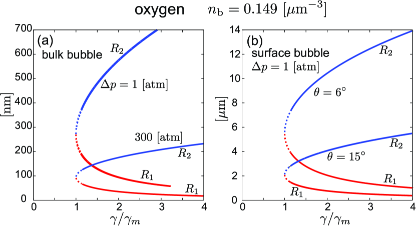
Figure 3: (Color online) Two radii $R_{1}$ and $R_{2}$ vs $\gamma/\gamma_{\rm m}$ giving the local maximum and minimum of $\Delta G$ for O₂ in water at $T=300$ K in the isobaric condition. They are written in dotted lines in the region $\gamma_{\rm m}<\gamma<\gamma_{\rm tr}$. As in Fig.2, displayed curves are for bulk bubbles with $\Delta p={\bar{p}}-p_{\rm cx}$ being 1 or 300 atm (left) or for surface bubbles with $\theta=15^{\circ}$ or $6^{\circ}$ (right).

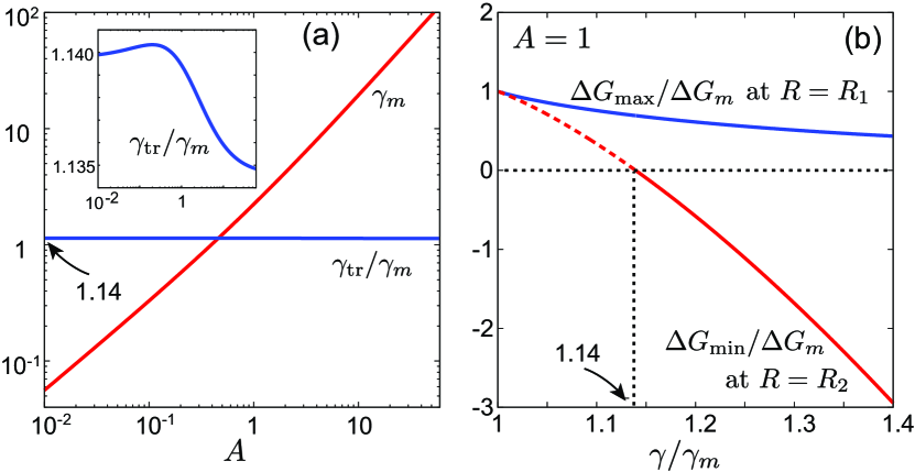
Figure 4: (Color online) (a) $\gamma_{\rm m}(A)$ and ratio $\gamma_{\rm tr}(A)/\gamma_{\rm m}(A)$ vs $A$ in the isobaric condition, where $\Delta G(R,\gamma,A)$ as a function of $R$ exhibits local extrema for $\gamma>\gamma_{\rm m}$ and its local minimum becomes negative for $\gamma>\gamma_{\rm tr}$. Here, $\gamma_{\rm tr}/\gamma_{\rm m}\cong 1.14$ for any $A$. (b) Local maximum $\Delta G_{\rm max}(\gamma,A)$ at $R=R_{1}$ and local minimum $\Delta G_{\rm min}(\gamma,A)$ at $R=R_{2}$ divided by $\Delta G_{\rm m}(\gamma_{\rm m},A)$ as functions of $\gamma/\gamma_{\rm m}$ for $A=1$. Here, $\Delta G_{\rm min}<0$ for $\gamma>\gamma_{\rm tr}$, where $R_{2}$ is the equilibrium bubble radius.

Furthermore, if we assume the pressure balance (21) (without assuming eq.(14)), $\Delta G$ becomes a function of $R$ only under eqs.(28) and (35). Its derivative with respect to $R$ is calculated as

$$\frac{d(\Delta G)}{dR}=S\bigg{[}\ln\bigg{(}\frac{n_{\rm I}^{\prime}}{\hat{n}_{\rm I}}\bigg{)}-\Delta\nu_{\rm s}\bigg{]}\bigg{[}{\bar{p}}-p_{\rm cx}+\frac{4\sigma}{3R}\bigg{]}$$ (39)

The extremum condition ${d(\Delta G)}/{dR}=0$ gives $n_{\rm I}^{\prime}={\hat{n}}_{\rm I}e^{\Delta\nu_{\rm s}}$, leading to eqs.(14) and (15).

III.2 Local maximum and minimum of bubble free energy at fixed pressure

In Fig.2, we plot $\Delta G/N_{\rm b}k_{B}T$ vs $R$ for O₂ for bulk and surface bubbles in water under eq.(21), where $T=300$ K and ${\bar{p}}-p_{\rm cx}=1$ or 300 atm. When we use O₂ (in Figs.2, 3, 6, and 7), we fix the bubble density at $n_{\rm b}=N_{\rm b}/V=0.149/$$\mu$m³. We recognize that $\Delta G$ assumes a local maximum at $R=R_{1}$ and a negative minimum at $R=R_{2}$ for sufficiently large ${\bar{n}}_{\rm I}$. Therefore, bubbles can appear in equilibrium at $R=R_{2}$ with increasing ${\bar{n}}_{\rm I}$. For the case ${\bar{p}}-p_{\rm cx}=$ 300 atm, the pressure in the bubble interior is also nearly equal to 300 atm for $R\gg 5$ nm and the interior oxygen density is $n_{\rm I}^{\prime}=7.2$ $/$nm³ from the ideal-gas formula ($p=nk_{B}T$). Instead, if we use the van der Waals equation of state ($p=nk_{B}T/(1-n/3n_{c})-(9k_{B}T_{c}/8n_{c})n^{2}$) at $p=300$ atm and $T=300$ K, the density becomes 7.9 $/$nm³, where $T_{c}=154.6$ K and $n_{c}=8.0$ nm^-3 for O₂. Thus, the van der Waals interaction among O₂ molecules is smaller than $k_{B}T$ (per molecule) even at ${\bar{p}}-p_{\rm cx}=300$ atm.

To explain Fig.2, we treat $\Delta G$ as a function of $R$ by increasing ${\bar{n}}_{\rm I}$ or $\gamma$ with the other parameters fixed. As will be shown in Appendix B, $\Delta G$ monotonically increases for $\gamma<\gamma_{\rm m}$ and exhibits a local maximum $\Delta G_{\rm max}$ at $R={R}_{1}$ and a local minimum $\Delta G_{\rm min}$ at $R=R_{2}$, where $\Delta G_{\rm min}>0$ for $\gamma_{\rm m}<\gamma<\gamma_{\rm tr}$ and $\Delta G_{\rm min}<0$ for $\gamma>\gamma_{\rm tr}$. Here, $R_{2}/R_{1}$ increases from 1 with increasing $\gamma$ above $\gamma_{\rm m}$. In each panel in Fig.2, we set $\gamma_{\rm m}<\gamma<\gamma_{\rm tr}$ for the upper curve, $\gamma=\gamma_{\rm tr}$ for the middle curve, and $\gamma>\gamma_{\rm tr}$ for the lower curve. Therefore, the two-phase states at $R=R_{2}$ are metastable for $\gamma_{\rm m}<\gamma<\gamma_{\rm tr}$ and stable for $\gamma\geq\gamma_{\rm tr}$. In Fig.3, we plot $R_{1}$ and $R_{2}$ for O₂ in water for bulk and surface bubbles.

In Appendix B, we shall see that $\gamma_{\rm m}$ and $\gamma_{\rm tr}$ depend only on the following dimensionless parameter,

$$A=[2\sigma/({\bar{p}}-p_{\rm cx})][4\pi G(\theta)n_{\rm b}e^{\Delta\nu_{\rm s}}/3]^{1/3},$$ (40)

which diverges as ${\bar{p}}\to p_{\rm cx}$ and becomes small with increasing ${\bar{p}}-p_{\rm cx}$ and/or decreasing $G(\theta)n_{\rm b}$. Using $A$, we may rewrite eq.(26) in terms of $u=R/R_{c}$ as

$$A^{3}u^{3}=\gamma^{4}(u-1)/(u+\gamma),$$ (41)

which holds for $u=R_{1}/R_{c}$ and $R_{2}/R_{c}$. In Fig.4, we plot $\gamma_{\rm m}$ and $\gamma_{\rm tr}$ vs $A$ in (a) and display $\Delta G_{\rm max}$ and $\Delta G_{\rm min}$ as functions of $\gamma/\gamma_{\rm m}$ at $A=1$ in (b). Here, $\gamma_{\rm m}\sim A^{3/4}$ for $A\ll 1$ and $\gamma_{\rm m}\sim A$ for $A\gg 1$. For any $A$, we find

$$\gamma_{\rm tr}/\gamma_{\rm m}\cong 1.14.$$ (42)

For example, $\gamma_{\rm m}=0.330,2.23,$ and 19.4 for $A=0.1$, 1, and 10, respectively. The threshold of bubble formation $(\gamma>\gamma_{\rm tr})$ is thus approximately given by ${\bar{n}}_{\rm I}\gtrsim{n}_{\rm I}^{c}$ for $A\lesssim 1$ and by ${\bar{n}}_{\rm I}\gtrsim A{n}_{\rm I}^{c}$ for $A\gtrsim 1$.

In particular, with increasing the solute density, we examine the case $\gamma\gg\gamma_{\rm m}\sim\gamma_{\rm tr}$ using eq.(41), where $R_{2}$ is the equilibrium radius. Then, for any $A$, we find

$$R_{1}/R_{c}\cong 1+A^{3}(1+\gamma)/\gamma^{4}+\cdots\cong 1.$$ (43)

The ratio $R_{1}/R_{c}$ rapidly approaches $1$ with increasing $\gamma$. In fact, even at $\gamma=\gamma_{\rm tr}$, we have $R_{1}/R_{c}=1.091$, 1.122, and 1.150 for $A=0.1$, 1, and 10, respectively. On the other hand, supposing $u=R_{2}/R_{c}\gg 1$, we obtain $u^{2}(u+\gamma)\cong\gamma^{4}/A^{3}$ from eq.(41). For $A\ll 1$, we have

$$R_{2}/R_{c}\cong\gamma^{4/3}/A\gg 1.$$ (44)

For $A\gg 1$, there are two limiting cases:

$$R_{2}/R_{c} \cong (\gamma/A)^{3/2}\gg 1\quad(A\ll\gamma\ll A^{3})$$ (45)

$$\cong \gamma^{4/3}/A\gg\gamma\quad\quad(\gamma\gg A^{3}).$$ (46)

In these limiting cases, we surely obtain $R_{2}\gg R_{c}$. See Fig.10 in Appendix B for the behaviors of $R_{1}$ and $R_{2}$ vs $\gamma$. On the other hand, for $\gamma\gg\gamma_{\rm m}$, the solute fraction $\alpha$ in bubbles in eq.(16) is much smaller than 1 at $R=R_{1}$ and approaches 1 at $R=R_{2}$ (see Fig.10(b)).

III.3 Bubble free energy at fixed chemical potentials

So far we have fixed the total particle numbers $N=V({\hat{n}}+\phi n^{\prime})$ and $N_{\rm I}=V({\hat{n}}_{\rm I}+\phi n_{\rm I}^{\prime})$ as well as the liquid pressure. In this case, the water chemical potential $\hat{\mu}$ is nearly fixed at the initial value ${\bar{\mu}}$ from eq.(18). As another boundary condition, we may attach a solute reservoir to the cell to fix the solute chemical potential at the initial value ${\bar{\mu}}_{\rm I}$, where we still attach a pressure valve. In this grand canonical case, we have ${\hat{n}}_{\rm I}={\bar{n}}_{\rm I}$ so that ${\hat{\omega}}=0$ from eq.(32). We should minimize the grand potential,

$$\Omega = G-{\bar{\mu}}N-{\bar{\mu}}_{\rm I}N_{\rm I}$$ (47)

$$= V\phi\omega^{\prime}+\sigma S,$$

where $G$ is defined in eq.(31), ${\bar{\mu}}$ and ${\bar{\mu}}_{\rm I}$ are the initial chemical potentials, and $\omega^{\prime}$ is given by eq.(36). To derive the second line of eq.(47), we have used the relation ${F}/{V}=\phi\omega^{\prime}-(1+\phi){\bar{p}}+{\bar{\mu}}(\hat{n}+\phi n^{\prime})+{\bar{\mu}}_{\rm I}({\hat{n}}_{\rm I}+\phi n_{\rm I}^{\prime})$, where $N$ and $N_{\rm I}$ are not fixed.

With respect to small changes $n_{\rm I}^{\prime}\to n_{\rm I}^{\prime}+\delta n_{\rm I}^{\prime}$ and $\phi\to\phi+\delta\phi$, the incremental change of $\Omega$ is given by the right hand side of eq.(38) if ${\hat{n}}_{\rm I}$ is replaced by ${\bar{n}}_{\rm I}$. Therefore, the extremum conditions $\partial\Omega/\partial n_{\rm I}^{\prime}=\partial\Omega/\partial\phi=0$ yield the pressure balance (21) and the chemical equilibrium condition ${n}^{\prime}_{\rm I}={\bar{n}}_{\rm I}e^{\Delta\nu_{\rm s}}$. If these extremum conditions are assumed, we obtain

$$\omega^{\prime}=-({\bar{p}}-p_{\rm cx})\gamma,$$ (48)

which is negative for $\gamma>0$ outside CX. Here, in the second line of eq.(47), the first term is proportional to $R^{3}$ and the second term to $R^{2}$, so the minimum of $\Omega$ decreases monotonically with increasing $R$ (for $R>R_{c}$), indicating appearance of macroscopic bubbles.

IV Solute-induced nucleation

IV.1 Experimental situations

We have shown that the bubble free energy $\Delta G(R)$ has a local maximum at $R=R_{1}$ and a minimum at $R=R_{2}$ for $\gamma>\gamma_{\rm tr}$ (except for gas films). In such situations, the initial homogeneous state is metastable and there can be solute-induced bubble nucleation outside CX Onukibook . In contrast, in one-component fluids, bubble nucleation occurs only inside CX (${\bar{p}}<p_{\rm cx}$) Katz ; Caupin ; Binder ; hetero ; Onukibook . In nucleation, crucial is the free energy $F_{c}$ needed to create a critical bubble with $R=R_{c}$. We call it the nucleation barrier, since the nucleation rate $I$ of bubble formation is proportional to the Boltzmann factor $\exp(-F_{c}/k_{B}T)$. Therefore, if $F_{c}/k_{B}T$ is too large (say, 80), $I$ becomes too small for experiments on realistic timescales. In our case, $F_{c}$ is reduced with increasing ${\bar{p}}-p_{\rm cx}$ and/or $\gamma={\bar{n}}_{\rm I}/{n}_{\rm I}^{c}-1$. For surface bubbles, it is also reduced with decreasing the contact angle $\theta$.

We make some comments on experimental situations. First, in the previous observations Bunkin ; ex2 ; ex3 ; ex4 , bulk nanobubbles have been produced by breakup of large bubbles composed of a gas such as O₂, CH₄, or Ar, where the typical flow-induced bubble size is of great interest Onukishear . Second, a small amount of surfactants and/or ions are usually present in water, which increase the bubble stability review2 . Indeed, surfactant molecules at the gas-liquid interface reduce the surface tension, while electric charges or electric double layers at the interface prevent bubble coalescence salt ; salt1 ; Grac ; Takahashi . For example, with addition of O₂ and a salt in waterex3 , the bubble-size distribution on long timescales was found to have a peak at $R\sim 100$ nm. Third, on a non-smooth hydrophobic wall, there can be preexisting trapped bubbles or strongly hydrophobic spots. In such cases, there should be no significant nucleation barrier for the formation of surface bubbles with small contact angles $\theta$.

IV.2 Critical radius and nucleation barrier

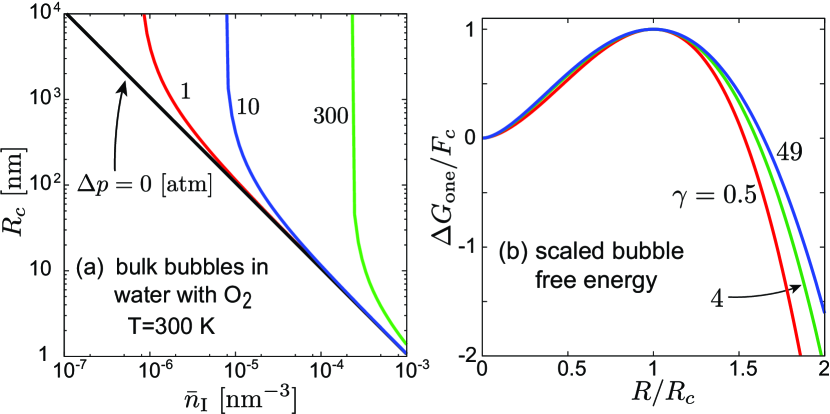
Figure 5: (Color online) (a) Critical radius $R_{c}$ in eq.(27) vs oxygen density ${\bar{n}}_{\rm I}$ for bulk bubbles in water, where $\Delta p={\bar{p}}-p_{\rm cx}=0,10$, and 300 atom and $T=300$ K. (b) $\Delta G_{\rm one}(R)/F_{c}$ in eq.(51) vs $R/R_{c}$ for $\gamma=0.5,4,$ and 49.

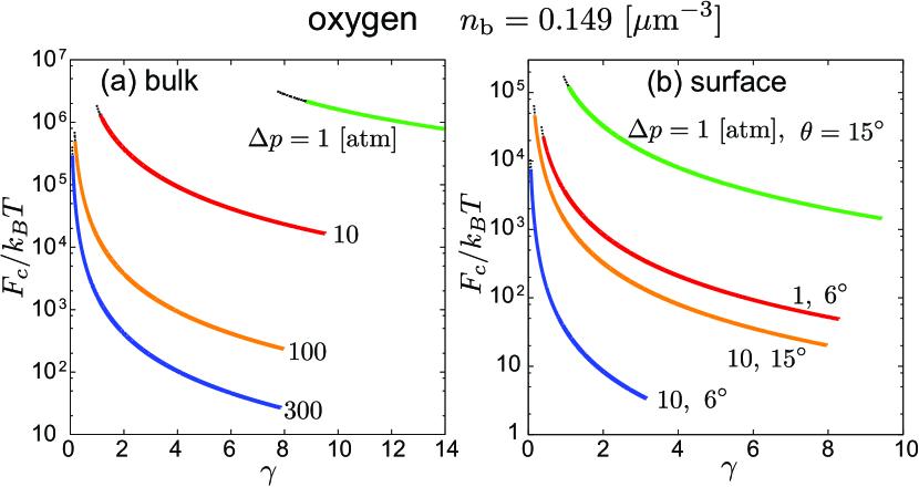
Figure 6: (Color online) Normalized nucleation barrier $F_{c}/k_{B}T$ vs $\gamma$ for O₂ in water. for (a) bulk and (b) surface bubbles.

We consider a single bubble with curvature $R^{-1}$ in bulk or on a hydrophobic wall. In the early stage with small $\phi$, we may neglect $\hat{\omega}\propto\phi^{2}$ in eq.(34) to obtain the single-bubble free energy in the standard form Caupin ; Binder ; hetero ; Onukibook ; Katz ,

$$\Delta G_{\rm one}(R)=G(\theta)\bigg{[}\frac{4}{3}\pi R^{3}\omega^{\prime}+4\pi\sigma R^{2}\bigg{]},$$ (49)

where $\omega^{\prime}$ is given by eq.(36) and $n_{\rm I}^{\prime}$ is related to $R$ by the pressure balance (21). Note that $\omega^{\prime}$ is usually a negative constant in nucleation in metastable systems. Here, $d(\Delta G_{\rm one})/dR\propto\ln(n_{\rm I}^{\prime}/{\bar{n}}_{\rm I})-\Delta\nu_{\rm s}$, which follows from eq.(39) if ${\hat{n}}_{\rm I}$ is replaced by ${\bar{n}}_{\rm I}$. Then, $\Delta G_{\rm one}(R)$ is maximized at the critical radius $R_{c}$ in eq.(27). See Fig.5(a) for $R_{c}$ vs ${\bar{n}}_{\rm I}$ for O₂. Since $\omega^{\prime}=-2\sigma/R_{c}$ at $R=R_{c}$ from eq.(36), the nucleation barrier ($=$the maximum of $\Delta G_{\rm one}$ at $R=R_{c}$) is written as

$$F_{c}=4\pi G(\theta)\sigma R_{c}^{2}/3=16\pi G(\theta)\sigma^{3}/[({\bar{p}}-p_{\rm cx})\gamma]^{2}.$$ (50)

For surface bubbles with small $\theta$, we have $G(\theta)\cong 3\theta^{4}/16$ and $G_{c}\propto\theta^{4}$. For bubble nucleation in one-component fluids, $F_{c}$ is given by the above form with $\gamma=1$ and ${\bar{p}}<p_{\rm cx}$. In terms of $u=R/R_{c}$, we may also express $\Delta F_{\rm one}(R)$ simply as

$$\Delta G_{\rm one}/F_{c}=2u^{2}(u/\gamma+1)\ln\bigg{(}\frac{1+\gamma/u}{1+\gamma}\bigg{)}+u^{2}.$$ (51)

The right hand side may be approximated by $-2u^{3}+3u^{2}$ for $\gamma\ll 1$ and by $-2u^{2}\ln u+u^{2}$ for $\gamma\gg 1$. In Fig.5(b), we plot the above scaling function. In addition, the nucleation rate $I$ is of the form Onukibook

$$I=\Gamma_{c}n_{\rm cx}^{\ell}\exp(-F_{c}/k_{B}T),$$ (52)

where $\Gamma_{c}$ is the growth rate of a critical bubble (see eq.(60) in the next subsection).

For water at $T=300$ K, we have

$$F_{c}/k_{B}T\cong 73G(\theta)R_{c}^{2},$$ (53)

with $R$ in nm. In Fig.6, we plot $F_{c}/k_{B}T$ vs ${\gamma}$ for O₂ in water for bulk and surface bubbles. . In homogeneous bubble nucleation of pure water at $T\sim 300$ K Katz ; Caupin , bubbles with $R>R_{c}$ are detectable for $F_{c}/k_{B}T\lesssim 70$ or for $R_{c}\lesssim 1$ nm in experimental times and $R_{c}$ can be of order 1 nm only for negative ${\bar{p}}$ of order $-1000$ atom. For O₂ in our case, $R_{c}$ is decreased down to 1 nm, depending on ${\bar{n}}_{\rm I}$, ${\bar{p}}-p_{\rm cx}$, and $\theta$ in Fig.6.

IV.3 Dynamics of bulk nucleation

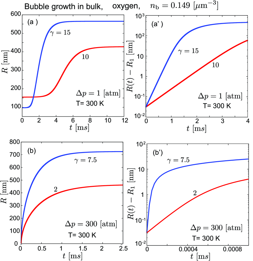
Figure 7: (Color online) Growth of radius $R(t)$ for bulk bubbles in the isobaric condition for O₂ in water at $T=300$ K, which are obtained from eq.(59) for $R(0)=R_{1}+0.3$ ${\rm\AA}$ with $D=2\times 10^{-9}$ cm${}^{2}/$s. In (a) and (a’), $\gamma=10$ and 15 with $\Delta p={\bar{p}}-p_{\rm cx}=$1 atom. In (b) and (b’), $\gamma=2$ and 7.5 with $\Delta p=$300 atm. Curves are written on linear scales in (a) and (b) and on semi-logarithmic scales in (a’) and (b’). Here, $\gamma_{\rm tr}=8.80$ and $0.0774$ for $\Delta p=1$ and $300$ atm, respectively.

We next examine nucleation dynamics of bulk bubbles for $\gamma>\gamma_{\rm tr}$. To describe attainment of the equilibrium radius $R_{2}$ in the simplest manner, we assume a common radius $R(t)$ for all the bubbles with a constant bubble density $n_{\rm b}$. We also assume a time-dependent background solute density in the liquid defined by

$$\hat{n}_{\rm I}(t)={\bar{n}}_{\rm I}-\phi(t)n_{\rm I}^{\prime}(t),$$ (54)

where $\phi(t)$ is determined by eq.(28) with $G(\theta)=1$. Expressing $\phi(t)$ and $n_{\rm I}^{\prime}(t)$ in terms of $R(t)$, we may describe saturation of $\phi(t)$ up to the equilibrium volume fraction. After this stage, however, the bubble number decreases in time in the presence of bubble coalescence (which can be suppressed with addition of saltsalt ; salt1 ).

For simplicity, we further assume that the solute diffusion constant $D$ is much smaller than the thermal diffusion constant $D_{T}$ in the liquid. Then, we can neglect temperature inhomogeneity around bubbles, which much simplifies the calculation. In fact, for liquid water at $300$ K and 1 atom, we have $D_{T}\sim 1.4\times 10^{-3}$ cm${}^{2}/$s and $D\sim 2.0\times 10^{-5}$ cm${}^{2}/$s ($\ll D_{T}$) for O₂.

We focus our attention to a single bubble neglecting its Brownian motion, where $n_{\rm I}(r,t)$ slowly changes in time $t$ tending to ${\hat{n}}_{\rm I}(t)$ in eq.(54) far from it. We write the distance from the droplet center as $r$. In the bubble exterior $r>R$, the solute obeys the diffusion equation,

$$\frac{\partial n_{\rm I}}{\partial t}=D\nabla^{2}n_{\rm I}.$$ (55)

We assume the continuity of the solute chemical potential $\mu_{\rm I}$ at $r=R+0$ and $r=R-0$ across the interface. From eq.(7), the solute density $n_{\rm I}^{R}=n_{\rm I}(R+0,t)$ immediately outside the bubble is related to the interior density $n_{\rm I}^{\prime}$ by

$$n_{\rm I}^{R}=n_{\rm I}^{\prime}e^{-{\Delta\nu}_{s}}.$$ (56)

Therefore, in the quasi-static approximationOnukibook , $n_{\rm I}(r,t)$ slightly outside the interface is written as

$$n_{\rm I}(r,t)={\hat{n}}_{\rm I}+({n}_{\rm I}^{R}-{\hat{n}}_{\rm I})R/r.$$ (57)

The flux to the bubble is given by $D({\hat{n}}_{\rm I}-{n}_{\rm I}^{R})/R$, so the conservation of the solute yields

$$({n}_{\rm I}^{\prime}-{n}_{\rm I}^{R})\frac{dR}{dt}=\frac{D}{R}({\hat{n}}_{\rm I}-n_{\rm I}^{R})$$ (58)

Here, ${\hat{n}}_{\rm I}-n_{\rm I}^{R}={\bar{n}}_{\rm I}-n_{\rm I}^{\prime}(\phi+e^{-\Delta\nu_{\rm s}})$ from eqs.(13) and (55, so the right hand side of eq.(58) vanishes at $R=R_{2}$ from eq.(13). In accord with the equilibrium relation (27), division of eq.(58) by $n_{\rm I}^{\prime}D/R$ gives the desired equation,

$$(1-e^{-{\Delta\nu}_{s}})\frac{R}{D}\frac{dR}{dt}=\frac{({\bar{n}}_{\rm I}-n_{\rm I}^{c})(1-R_{c}/R)}{({\bar{p}}-p_{\rm cx}+2\sigma/R)/k_{B}T}-\phi.$$ (59)

For $\gamma>\gamma_{\rm tr}$, the right hand side of eq.(59) vanishes for $R=R_{1}$ and $R_{2}$, where $R_{1}\cong R_{c}$. Here, bubbles with $R>R_{1}$ grow up to $R_{2}$, while those with $R<R_{1}$ shrink. If the deviation $\delta R=R-R_{1}$ is small, it obeys the linear equation $d(\delta R)/dt=\Gamma_{c}\delta R$, where $\Gamma_{c}$ is the growth rate of a critical bubble of the form,

$$\Gamma_{c}=DR_{c}^{-2}\gamma/[(1+\gamma)(e^{\Delta\nu_{\rm s}}-1)].$$ (60)

In terms of $\Gamma_{c}$ and $u=R/R_{c}$, we may rewrite eq.(59) as

$$\frac{du}{dt}={\Gamma_{c}}\frac{1+\gamma}{u}\bigg{[}\frac{u-1}{u+\gamma}-\frac{A^{3}}{\gamma^{4}}u^{3}\bigg{]},$$ (61)

which is consistent with eq.(41).

In Fig.7, we display the growth of $R(t)$ by setting $D=2\times 10^{-5}$ cm${}^{2}/$s for O₂ in water at $T=300$ K, where ${\bar{p}}-p_{\rm cx}$ is 1 atm in (a) and (a’) and 300 atm in (b) and (b’). As the initial radius, we set $R(0)=R_{1}+0.3$ ${\rm\AA}$, which yields $u(0)-R_{1}/R_{c}\sim 10^{-2}$ in eq.(61). The right panels indicate the exponential growth,

$$R(t)=R(0)+(R(0)-R_{1})e^{\Gamma_{c}t}$$ (62)

in the early stage. Numerically, $\Gamma_{c}$ is $2.89$ and $6.70$ for $\gamma=10$ and 15, respectively, in (a) and (a’), while it is $7.63$ and $142$ for $\gamma=2$ and 7.5, respectively, in (b) and (b’). These values agree with eq.(59). In this calculation, we assume the pre-existence of bubbles with radii slightly exceeding $R_{1}$. However, if we start with the homogeneous initial state, the birth of such large bubbles in the cell occurs as rare thermal activations on a timescale of order,

$$1/VI\sim\exp({F_{c}/k_{B}T})/Vn_{\rm cx}^{\ell}\Gamma_{c}.$$ (63)

V Summary

We have investigated bubble formation in bulk and on hydrophobic walls induced by accumulation of a small amount of a neutral solute in liquid water outside the solvent CX. We have used the fact that a gas such as O₂ or N₂ remains in gaseous states within phase-separated domains in ambient liquid water, because it is mildly hydrophobic with a critical temperature much below 300 K. With this input, we have constructed a simple thermodynamic theory for dilute binary mixtures including a considerably large solvation chemical potential difference $\Delta\mu_{\rm s}=k_{B}T\Delta\nu_{\rm s}$. We have assumed fixed particle numbers and a fixed liquid pressure $(N$-$N_{\rm I}$-$p)$ in the text and in Appendix B, but we have also treated bubble formation in the $\mu$-$\mu_{\rm I}$-$p$ ensemble in Sec.IIIC and in the $N$-$N_{\rm I}$-$V$ ensemble in Appendices A and B,

In particular, in Sec.II, we have found a threshold solute density $n_{\rm I}^{c}$ in eq.(23) for film formation on a completely dried wall at fixed pressure, which is very small for large $\Delta\nu_{\rm s}$. The threshold density is increased to $(\gamma_{\rm m}+1)n_{\rm I}^{c}$ for metastable bubbles and $(\gamma_{\rm tr}+1)n_{\rm I}^{c}$ for stable bubbles due to the surface tension, where $\gamma_{\rm tr}\cong 1.14\gamma_{\rm m}$. Here, $\gamma_{\rm m}$ and $\gamma_{\rm tr}$ are displayed in Fig.4(a) as functions of a parameter $A$ in eq.(40). In Sec.III, we have also presented a bubble free energy $\Delta G$ for a small gas fraction $\phi$ in eqs.(34)-(37) for the isobaric case, whose minimization yields the equilibrium conditions (14) and (21). In Sec,IV, we have calculated the critical radius $R_{c}$ and the barrier free energy $F_{c}$ for solute-induced nucleation. The $F_{c}/k_{B}T$ is very high for homogeneous nucleation except for high liquid pressures, but it can be decreased for heterogeneous nucleation with a small contact angle $\theta$.

We make some critical remarks. (i) First, we have assumed gaseous domains. However, with increasing ${\bar{p}}-p_{\rm cx}$ and/or $\Delta\nu_{\rm s}$, liquid or solid precipitates should be formed in bulk and on walls, sensitively depending on their mutual attractive interaction. Note that a large attractive interaction arises even among large hard-sphere particles in water due to deformations of the hydrogen bonding Paul ; Garde ; Chandler ; Pratt . (ii) Second, we should include the effects of surfactants and ions in the discussion of the bubble size distribution review2 ; salt ; salt1 ; Grac ; Takahashi . In this paper, we have assumed a constant bubble density $n_{\rm b}$ in eqs.(28), (35), and (40). This assumption can be justified only when bubble coalescence is suppressed by the electrostatic interaction near the gas-liquid interfaces. (iii) Third, dynamics of bubble formation and dissolutionTeshi should be studied in future, which can be induced by a change in pressure, temperature, or solute density.

$${\hat{n}}=(1+\phi){\bar{n}}.$$ (A1)

In terms of the isothermal compressibility $K_{T}$ of liquid water, the pressure increase is given by $\phi/K_{T}$, so the pressure balance relation (21) is changed as

$$k_{B}Tn_{\rm I}^{\prime}={\bar{p}}-p_{\rm cx}+\phi/K_{T}+2\sigma/R.$$ (A2)

Here, $K_{T}=0.45\times 10^{-3}/$MPa in ambient water near CX, where even a very small $\phi$ gives rise to a large pressure.

The bubble free energy $\Delta F$ is defined as the increase in the Helmholtz free energy as $F={\bar{F}}+\Delta F$ due to appearance of bubbles. Some calculations give

$$\Delta F=V[\phi\omega^{\prime}+(1-\phi)\hat{\omega}]+\sigma S.$$ (A3)

Here, we may replace $(1-\phi)\hat{\omega}$ by $\hat{\omega}$ for small $\phi$. Then $\Delta F$ assumes the form of eq.(34), but we need to change $\hat{\omega}$ in eq.(37) as

$$\hat{\omega}=T[{\hat{n}}_{\rm I}\ln({\hat{n}}_{\rm I}/{{\bar{n}}_{\rm I}})+\phi n_{\rm I}^{\prime}]+{\phi^{2}}/{2K_{T}},$$ (A4)

where the last term is due to the compression in the liquid. From eq.(1), it is equal to $f_{\rm w}^{\prime\prime}({\bar{n}})(\hat{n}-{\bar{n}})^{2}/2$, where $f_{\rm w}^{\prime\prime}=\partial^{2}f_{\rm w}/\partial n^{2}=1/n^{2}K_{T}$. The counterpart of eq.(38) for the increment $\delta(\Delta F)$ is obtained if ${\bar{p}}-p_{\rm cx}$ is replaced by ${\bar{p}}-p_{\rm cx}+\phi/K_{T}$. Minimization of $\Delta F$ with respect to $\phi$ and $n_{\rm I}^{\prime}$ thus yields eqs.(14) and (A2). Furthermore, the derivative $d(\Delta F)/dR$ is obtained if ${\bar{p}}-p_{\rm cx}$ is replaced by ${\bar{p}}-p_{\rm cx}+2\phi/K_{T}$ in the right hand side of eq.(39).

The equilibrium equation for $R$ or $\phi$ is given by eq.(22) if ${\bar{p}}-p_{\rm cx}$ is replaced by ${\bar{p}}-p_{\rm cx}+\phi/K_{T}$. In particular, for a gas film $(R^{-1}=0$), $\phi$ is explicitly calculated as

$${\phi}=e^{-\Delta{\nu}_{s}}\bigg{[}\sqrt{(1+h)^{2}/4+\gamma h}-\frac{1+h}{2}\bigg{]},$$ (A5)

where we define

$$h=K_{T}({\bar{p}}-p_{\rm cx})e^{\Delta\nu_{\rm s}}.$$ (A6)

For O₂ in ambient water, we have $h=1.4\times 10^{-3}({\bar{p}}-p_{\rm cx})$ with pressures in atm, so $h\ll 1$ for ${\bar{p}}\ll 10^{3}$ atm.

Here, we assume $1+h>0$. A film appears for $\gamma>0$ as in the isobaric case. In particular, for $\gamma|h|\ll(1+h)^{2}/4$, we find the linear behavior $\propto\gamma$ as

$$\phi \cong \gamma e^{-\Delta\nu_{\rm s}}{h}/({1+h})$$ (A7)

$$\cong \frac{K_{T}}{1+h}\bigg{[}k_{B}T{\bar{n}}_{\rm I}e^{\Delta\nu_{\rm s}}-{\bar{p}}+p_{\rm cx}\bigg{]}.$$

From the first line, this formula tends to eq.(25) only for $h\gg 1$. The second line can be used even for ${\bar{p}}\leq p_{\rm cx}$, where $\phi$ increases with increasing $p_{\rm cx}-{\bar{p}}$ and/or ${\bar{n}}_{\rm I}$. See Appendix B for more analysis for the case $R^{-1}>0$.

Appendix B: Scaling of bubble free energy

Here, we examine the bubble free energy $\Delta F$ in eq.(34) by scaling it in a dimensionless form, assuming a common curvature $R^{-1}$ for all the bubbles.

1. Fixed pressure
At fixed pressure in Fig.1, we assume the pressure balance (21) and introduce scaling variables $s$ and $v$ by

$$s = \phi e^{\Delta\nu_{\rm s}}=(4\pi G(\theta)n_{\rm b}/3)e^{\Delta\nu_{\rm s}}R^{3},$$ (B1)

$$v = [2\sigma/({\bar{p}}-p_{\rm cx})R]=As^{-1/3}.$$ (B2)

where $A$ is the parameter in eq.(40). From eq.(16) the solute fraction in bubbles is $\alpha=s/(1+s)$. As a scaled bubble free energy, we define $\cal F$ as

$${\cal F}=e^{\Delta\nu_{\rm s}}\Delta G/[V({\bar{p}}-p_{\rm cx})].$$ (B3)

From eqs.(34)-(37), we express $\cal F$ in terms of $s$ and $v$ as

$${\cal F}=[\gamma+1-s(1+{v})]\ln\bigg{[}1-s\frac{1+{v}}{1+\gamma}\bigg{]}$$

$$+s(1+{v})\ln\bigg{[}\frac{1+{v}}{1+\gamma}\bigg{]}++\frac{3}{2}sv+s,$$ (B4)

where $\gamma$ is given by eq.(24). With fixed $\gamma$ and $A$, $\cal F$ is a function of $s$ only. From eq.(B2) its derivative with respect to $s$ is calculated as

$$\frac{\partial}{\partial s}{\cal F}=\bigg{(}1+\frac{2}{3}v\bigg{)}\ln\bigg{[}\frac{1+v}{\gamma+1-s(1+v)}\bigg{]}.$$ (B5)

The extremum condition ${\partial}{\cal F}/\partial s=0$ yields

$$\gamma=s+(1+s)v=s+A(1+s)s^{-1/3},$$ (B6)

which is equivalent to eqs.(21), (26), and (41). If eq.(B6) is assumed, we have ${\cal F}=(3v/2+1)s-(1+\gamma)\ln(1+s)$ as extremum values depending only on $A$. In Fig.8, we display ${\cal F}(\gamma,s,A)$ in the $\gamma$-$s$ plane at $A=1$.

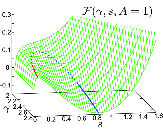
Figure 8: (Color online) ${\cal F}$ in the isobaric condition in the $\gamma$-$s$ plane at $A=1$ in the neighborhood of $\gamma=\gamma_{\rm m}$ and $s=s_{\rm m}$. Curve of $(\partial{\cal F}/\partial s)_{\gamma}=0$ or eq.(B6) is written on the surface, on which $s=s_{1}(\gamma,A)$ for the local maximum and $s=s_{2}(\gamma,A)$ for the local minimum for each $\gamma$.

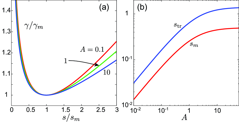
Figure 9: (Color online) Results in the isobaric condition. (a) $\gamma/\gamma_{\rm m}$ vs $s/s_{\rm m}$ from the extremum condition (B6) for $A=0.1$, 1, and 10 and (b) $s_{\rm m}$ and $s_{\rm tr}$ vs $A$. Here, $\gamma_{\rm m}$, $s_{\rm m}$, and $s_{\rm tr}$ are determined by eqs.(B7)-(B9).

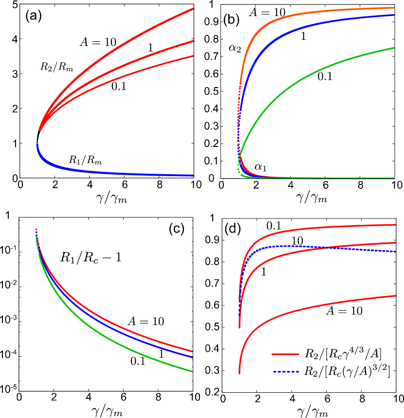
Figure 10: (Color online) Results in the isobaric condition. (a) $R_{1}/R_{\rm m}=(s_{1}/s_{\rm m})^{1/3}$ and $R_{2}/R_{\rm m}=(s_{2}/s_{\rm m})^{1/3}$ vs $\gamma/\gamma_{\rm m}$ and (b) $\alpha_{1}=s_{1}/(1+s_{1})$ and $\alpha_{2}=s_{2}/(1+s_{2})$ vs $\gamma/\gamma_{\rm m}$, where $A=0.1,1$, and 10. (c) $R_{1}/R_{c}-1=s_{1}^{1/3}\gamma/A-1$ vs $\gamma/\gamma_{\rm m}$, which is small even for vs $\gamma=\gamma_{\rm tr}$ (see eq.(43)). (d) $R_{2}/[R_{c}\gamma^{4/3}/A]$ for $A=0.1$, 1, and 10 (bold lines) and $R_{2}/[R_{c}(\gamma/A)^{3/2}]$ for $A=10$ (dotted line) as functions of $\gamma/\gamma_{\rm m}$ (see eqs.(44)-(46)).

For each $A$, the right hand side of eq.(B6) is minimized at $s=s_{\rm m}(A)$ as a function of $s$, where $s_{\rm m}$ satisfies

$$A=3s_{\rm m}^{4/3}/(1-2s_{\rm m}).$$ (B7)

The minimum of eq.(B6) at $s=s_{\rm m}$ is written as

$$\gamma_{\rm m}=s_{\rm m}(4+s_{\rm m})/(1-2s_{\rm m}).$$ (B8)

As can be seen in Fig.9(a), if $\gamma>\gamma_{\rm m}$, eq.(B6) has two solutions $s_{1}(\gamma,A)$ and $s_{2}(\gamma,A)$ with $s_{1}\leq s_{2}$, where ${\cal F}(s,\gamma,A)$ exhibits a local maximum ${\cal F}_{\rm max}(\gamma,A)$ at $s=s_{1}$ and a local minimum ${\cal F}_{\rm min}(\gamma,A)$ at $s=s_{2}$. Further increasing $\gamma$ above $\gamma_{\rm m}$, the local minimum ${\cal F}_{\rm min}$ decreases and becomes negative for $\gamma>\gamma_{\rm tr}(A)$, where $\gamma_{\rm tr}$ and the corresponding $s$, written as $s_{\rm tr}(A)$, are calculated from

$$A/(A+s_{\rm tr}^{1/3})=2(1+s_{\rm tr}^{-1})\ln(1+s_{\rm tr})-2,$$ (B9)

$$\gamma_{\rm tr}=s_{\rm tr}+A(1+s_{\rm tr})/s_{\rm tr}^{1/3}.$$ (B10)

See Fig.4(a) for $\gamma_{\rm m}$ and $\gamma_{\rm tr}/\gamma_{\rm m}(\cong 1.14)$ vs $A$.

From eqs.(B7)-(B10), we seek the asymptotic behaviors for small and large $A$. For $A\ll 1$ we find

$$s_{\rm m}\cong(A/3)^{3/4},\quad~{}s_{\rm tr}\cong A^{3/4}$$

$$\gamma_{\rm m}\cong 4(A/3)^{3/4},\quad\gamma_{\rm tr}\cong 2A^{3/4}.$$ (B11)

On the other hand, for $A\gg 1$, we have

$$s_{m}\cong 1/2,\quad\quad~{}~{}~{}~{}~{}~{}s_{\rm tr}\cong 1.401$$

$$\gamma_{m}\cong(3/2^{2/3})A,\quad\gamma_{\rm tr}\cong 2.145A,$$ (B12)

where $s_{\rm tr}$ and $\gamma_{\rm tr}$ are calculated numerically. If $\gamma\gg\gamma_{\rm m}$, we obtain eqs.(43)-(46).

For $\gamma>\gamma_{\rm m}$, we consider the radii $R_{\rm m}$, $R_{1}$, and $R_{2}$ corresponding to $s_{\rm m},s_{1}$, and $s_{2}$. From eq.(B2) we have

$$\frac{R_{\rm m}}{R_{0}}=s_{\rm m}^{1/3},\quad\frac{R_{1}}{R_{0}}=s_{1}^{1/3},\quad\frac{R_{2}}{R_{0}}=s_{2}^{1/3},$$ (B13)

where $R_{0}=2\sigma/[({\bar{p}}-p_{\rm cx})A]=R_{c}\gamma/A$. In Fig.10, we plot $R_{1}/R_{\rm m}=(s_{1}/s_{\rm m})^{1/3}$ and $R_{2}/R_{\rm m}=(s_{2}/s_{\rm m})^{1/3}$ vs $\gamma/\gamma_{\rm m}$ in (a) and $\alpha_{1}=s_{1}/(1+s_{1})$ and $\alpha_{2}=s_{2}/(1+s_{2})$ vs $\gamma/\gamma_{\rm m}$ in (b), where the latter are the solute fractions in bubbles at $R=R_{1}$ and $R_{2}$. Furthermore, in (c), $R_{1}/R_{c}-1$ is shown to be small for $\gamma$ slightly larger $\gamma_{\rm m}$ in accord with eq.(42). In (d), we divide $R_{2}/R_{c}$ by its asymptotic forms for $\gamma\gg\gamma_{\rm m}$ to confirm eqs.(44)-(46).

2. Fixed volume
We next scale the bubble free energy $\Delta F$ in the fixed-volume condition in Appendix A. We assume the pressure balance (A2) and use $\hat{\omega}$ in eq.(A4). Introducing the scaled bubble free energy $\cal F$ as in eq.(B3) (with replacement $\Delta G\to\Delta F$), we express it in terms of $s$ in eq.(B1), $v$ in eq.(B2), and

$$\hat{v}=(2\sigma/R+\phi/K_{T})/({\bar{p}}-p_{\rm cx})=v+s/h,$$ (B14)

where $h$ is defined in eq.(A6). Replacing $v$ by $\hat{v}$ in the first two terms in eq.(B4), we obtain

$${\cal F}=[\gamma+1-s(1+\hat{v})]\ln\bigg{[}1-s\frac{1+\hat{v}}{1+\gamma}\bigg{]}$$

$$+s(1+\hat{v})\ln\bigg{[}\frac{1+\hat{v}}{1+\gamma}\bigg{]}+\frac{3}{2}sv+s+\frac{s^{2}}{2h},$$ (B15)

where the last term arises from the compression term in eq.(A4). As in eq.(B5), the derivative of $\cal F$ with respect to $s$ is calculated as

$$\frac{\partial}{\partial s}{\cal F}=\bigg{(}1+\frac{2v}{3}+\frac{2s}{h}\bigg{)}\ln\bigg{[}\frac{1+\hat{v}}{\gamma+1-s(1+\hat{v})}\bigg{]}.$$ (B16)

The extremum condition ${\partial}{\cal F}/\partial s=0$ yields

$$\gamma = s+(1+s)\hat{v}$$ (B17)

$$= s+A(1+s)s^{-1/3}+(s+s^{2})/h,$$

As in the fixed pressure case, ${\cal F}(s,\gamma,A,h)$ exhibits a local maximum at $s=s_{1}(\gamma,A,h)$ and a local minimum at $s=s_{2}(\gamma,A,h)$ for $\gamma>\gamma_{\rm m}(A,h)$ and its local minimum becomes negative for $\gamma>\gamma_{\rm tr}(A,h)$. Note that the right hand side of eq.(B17) is minimized at $s=s_{\rm m}(A,h)$, where $s_{\rm m}$ is determined by

$$A=3s_{\rm m}^{4/3}[1+(1+2s_{\rm m})/h]/({1-2s_{\rm m}}).$$ (B18)

The corresponding minimum of eq.(B17) is written as

$$\gamma_{\rm m}=[4+s_{\rm m}+4(1+s_{\rm m})^{2}/h]s_{\rm m}/(1-2s_{\rm m})$$ (B19)

Here, we assunme $Ah\ll 1$, where $s_{\rm m}\sim(Ah)^{3/4}\ll 1$ from eq.(B18). In fact, for O₂ in ambient water, we obtain $Ah=0.010[n_{\rm b}G(\theta)]^{1/3}$ with $n_{\rm b}$ in units of $\mu$m^-3, which is independent of ${\bar{p}}-p_{\rm cx}$. Then, as in eq.(B11), we find the asymptotic behaviors,

$$s_{\rm m}\cong(Ah/3)^{3/4},\quad~{}s_{\rm tr}\cong(Ah)^{3/4}$$

$$\gamma_{\rm m}\cong 4(A/3)^{3/4}/h^{1/4},\quad\gamma_{\rm tr}\cong 2A^{3/4}/h^{1/4},$$ (B20)

where $\gamma_{\rm tr}/\gamma_{\rm m}\cong 1.14$. As in eqs.(43) and (44), the radii $R_{1}$ and $R_{2}$ behave for $\gamma\gg\gamma_{\rm m}$ as

$$R_{1}\cong R_{c},\quad R_{2}\cong R_{c}\gamma^{4/3}h^{1/3}/A\gg R_{c}.$$ (B21)

References

- (1) P. Attard, M. P. Moody, and J.W.G. Tyrrell, Physica A 314, 696 (2002).
- (2) J. R. T. Seddon, D. Lohse, W. A. Ducker, and V. S. J. Craig, Chem. Phys. Chem. 13, 2179 (2012).
- (3) M.A. Hampton and A.V. Nguyen, Advances in Colloid and Interface Science 154, 30 (2010).
- (4) R.M. Pashley, P.M. McGuiggan, B.W. Ninham, and D.F. Evans, Science 229, 1088 (1985).
- (5) H.K. Christenson and P.M. Claesson, ibid. 239, 390 (1988).
- (6) A. Carambassis, L. C. Jonker, P. Attard, and M. W. Rutland, Phys. Rev. Lett. 80, 5357 (1998).
- (7) R. F. Considine and C. J. Drummond, Langmuir 16, 631 (2000)
- (8) J. W. G. Tyrrell and P. Attard, Phys. Rev. Lett. 87, 176104 (2001).
- (9) V. Yaminsky and S. Ohnishi, Langmuir 19, 1970 (2003).
- (10) A. C. Simonsen, P. L. Hansen, B. Klsgen, J. Colloid Interface Sci. 273, 291 (2004).
- (11) X. H. Zhang, A. Quinn, and W. A. Ducker, Langmuir 24, 4756 (2008).
- (12) M. A. J. van Limbeek and J. R. T. Seddon, Langmuir 27, 8694 (2011).
- (13) F. Jin, J. Ye, L. Hong, H. Lam, and C. Wu, J. Phys. Chem. B 111, 2255 (2007).
- (14) N. Ishida, M. Sakamoto, M. Miyahara, and K. Higashitani, Langmuir 16, 5681 (2000).
- (15) N. F. Bunkin, N. V. Suyazov, A. V. Shkirin, P. S. Ignatiev, and K. V. Indukaev, J. Chem. Phys. 130, 134308 (2009).
- (16) K. Ohgaki, N. Q. Khanh, Y. Joden, A. Tsuji, T. Nakagawa, Chem. Eng. Sci. 65, 1296 (20010).
- (17) F. Y. Ushikubo, T. Furukawa, R. Nakagawa, M. Enari, Y. Makino, Y. Kawagoe, T.Shiina, and S. Oshita, Colloids and Surfaces A 361,31 (2010).
- (18) T. Uchida, S. Oshita, M. Ohmori, T. Tsuno, K. Soejima, S. Shinozaki, Y. Take, and K. Mitsuda, Nanoscale Research Letters 6, 295 (2011).
- (19) A. Ben-Naim and Y. Marcus, J. Chem. Phys.81, 2016 (1984).
- (20) B. Guillot and Y. Guissani, J. Chem. Phys. 99, 8075 (1993).
- (21) G. Hummer, S. Garde, A. E. Garca, and L. R. Pratt, Chem. Phys. 258, 349 (2000).
- (22) H.S. Ashbaugh and M. E. Paulaitis, J. Am. Chem. Soc. 123, 10721 (2001).
- (23) D. Chandler, Nature, 437, 640 (2005).
- (24) S. Rajamani, T.M. Truskett, and S. Garde, Proc. Natl. Acad. Sci. U.S.A. 102, 9475 (2005).
- (25) J. W. Cahn, J. Chem. Phys. 66 3667 (1977).
- (26) D. Bonn and D. Ross, Rep.Prog.Phys.64, 1085 (2001).
- (27) D. A. Doshi, E. B. Watkins, J. N. Israelachvili, and J. Majewski, Proc. Natl. Acad. Sci. U.S.A. 102, 9458 (2005).
- (28) A. Poynor, L. Hong, I. K. Robinson, S. Granick, Z. Zhang, and P. A. Fenter, Phys. Rev. Lett. 97, 266101 (2006).
- (29) M. Mezger, H. Reichert, S. Schder, J. Okasinski, H. Schrder, H. Dosch, D. Palms, J. Ralston, and V. Honkimki, Proc Natl Acad Sci USA 103, 18401 (2006).
- (30) A. F. Kostko, M. A. Anisimov, and J. V. Sengers, Phys. Rev. E 70, 026118 (2004).
- (31) R. Okamoto and A. Onuki, Phys. Rev. E 82, 051501 (2010).
- (32) A. Onuki and R. Okamoto, Curr. Opin. Colloid In. 16, 525 (2011).
- (33) R. Sander, Atmos. Chem. Phys. Discuss. 14,29615 (2014).
- (34) F.L. Smith and A.H. Harvey, Chemical Engineering Progress, AIChE, 103, 33 (2007).
- (35) M. Blander and J. Katz, AIChE J. 21, 833 (1975).
- (36) M. E. M. Azouzi, C. Ramboz, J.-F. Lenain, and F. Caupin, Nat. Phys. 9, 38 (2013).
- (37) A. Onuki, Phase Transition Dynamics (Cambridge University Press, Cambridge, 2002).
- (38) D. Turnbull, J. Chem. Phys. 18, 198 (1950).
- (39) D. Winter, P. Virnau, and K. Binder, Phys. Rev. Lett. 103, 225703 (2009).
- (40) R. R. Lessard and S. A. Zieminski, Ind. Eng. Chem. Fundam., 10,260 (1971).
- (41) V. S. J. Craig,’ B. W. Ninham, and R. M. Pashley, J. Phys. Chem. 97, 10192 (1993).
- (42) A. Graciaa, G. Morel, P. Saulnier, J. Lachaise, and R. S. Schechter, J. Colloid Interface Sci. 172, 131 (1995).
- (43) M. Takahashi, J. Phys. Chem. B 109, 21858 (2005).
- (44) A. Onuki, J. Phys.: Condens. Matter 9, 6119 (1997).
- (45) K. Binder, Physica A 319, 99 (2003).
- (46) R. Teshigawara and A. Onuki, Phys. Rev. E 84, 041602 (2011).