A Bounded $p$-norm Approximation of Max-Convolution for Sub-Quadratic Bayesian Inference on Additive Factors

Abstract

Max-convolution is an important problem closely resembling standard convolution; as such, max-convolution occurs frequently across many fields. Here we extend the method with fastest known worst-case runtime, which can be applied to nonnegative vectors by numerically approximating the Chebyshev norm $\|\cdot\|_{\infty}$, and use this approach to derive two numerically stable methods based on the idea of computing $p$-norms via fast convolution: The first method proposed, with runtime in $O(k\log(k)\log(\log(k)))$ (which is less than $18k\log(k)$ for any vectors that can be practically realized), uses the $p$-norm as a direct approximation of the Chebyshev norm. The second approach proposed, with runtime in $O(k\log(k))$ (although in practice both perform similarly), uses a novel null space projection method, which extracts information from a sequence of $p$-norms to estimate the maximum value in the vector (this is equivalent to querying a small number of moments from a distribution of bounded support in order to estimate the maximum). The $p$-norm approaches are compared to one another and are shown to compute an approximation of the Viterbi path in a hidden Markov model where the transition matrix is a Toeplitz matrix; the runtime of approximating the Viterbi path is thus reduced from $O(nk^{2})$ steps to $O(nk\log(k))$ steps in practice, and is demonstrated by inferring the U.S. unemployment rate from the S&P 500 stock index.

1 Introduction

Max-convolution occurs frequently in signal processing and Bayesian inference: it is used in image analysis (Ritter and Wilson, 2000), in network calculus (Boyer et al., 2013), in economic equilibrium analysis (Sun and Yang, 2002), and in a probabilistic variant of combinatoric generating functions, wherein information on a sum of values into their most probable constituent parts (e.g. identifying proteins from mass spectrometry (Serang et al., 2010; Serang, 2014)). Max-convolution operates on the semi-ring $(max,\times)$, meaning that it behaves identically to a standard convolution, except it employs a $\max$ operation in lieu of the $+$ operation in standard convolution (max-convolution is also equivalent to min-convolution, also called infimal convolution, which operates on the tropical semi-ring $(min,+)$). Due to the importance and ubiquity of max-convolution, substantial effort has been invested into highly optimized implementations (e.g., implementations of the quadratic method on GPUs; Zach et al., 2008).

Max-convolution can be defined using vectors (or discrete random variables, whose probability mass functions are analogous to nonnegative vectors) with the relationship $M=L+R$. Given the target sum $M=m$, the max-convolution finds the largest values $L[\ell]$ and $R[r]$ for which $m=\ell+r$.

$$M[m] = \max_{\ell,r:\,m=\ell+r}L[\ell]R[r]$$

$$= \max_{\ell}L[\ell]R[{m-\ell}]$$

$$= \left(L~{}*_{\max}~{}R\right)[m]$$

where $*_{\max}$ denotes the max-convolution operator. In probabilistic terms, this is equivalent to finding the highest probability of the joint events $\Pr(L=\ell,R=r)$ that would produce each possible value of the sum $M=L+R$ (note that in the probabilistic version, the vector $M$ would subsequently need to be normalized so that its sum is 1).

Although applications of max-convolution are numerous, only a small number of methods exist for solving it (Serang, 2015). These methods fall into two main categories, each with their own drawbacks: The first category consists of very accurate methods that are have worst-case runtimes either quadratic (Bussieck et al., 1994) or slightly more efficient than quadratic in the worst-case (Bremner et al., 2006). Conversely, the second type of method computes a numerical approximation to the desired result, but in $O(k\log_{2}(k))$ steps; however, no bound for the numerical accuracy of this method has been derived (Serang, 2015).

While the two approaches from the first category of methods for solving max-convolution do so by either using complicated sorting routines or by creating a bijection to an optimization problem, the numerical approach solves max-convolution by showing an equivalence between $*_{\max}$ and the process of first generating a vector $u^{(m)}$ for each index $m$ of the result (where $u^{(m)}[\ell]=L[\ell]R[{m-\ell}]$ for all in-bounds indices) and subsequently computing the maximum $M[m]=\max_{\ell}u^{(m)}[\ell]$. When $L$ and $R$ are nonnegative, the maximization over the vector $u^{(m)}$ can be computed exactly via the Chebyshev norm

$$M[m] = \max_{\ell}u^{(m)}[\ell]$$

$$= \lim_{p\to\infty}\|u^{(m)}\|_{p}$$

but requires $O(k^{2})$ steps (where $k$ is the length of vectors $L$ and $R$). However, once a fixed $p^{*}$-norm is chosen, the approximation corresponding to that $p^{*}$ can be computed by expanding the $p^{*}$-norm to yield

$$\lim_{p\to\infty}\|u^{(m)}\|_{p} = \lim_{p\to\infty}{\left(\sum_{\ell}{\left(u^{(m)}[\ell]\right)}^{p}\right)}^{\frac{1}{p}}$$

$$\approx {\left(\sum_{\ell}{\left(u^{(m)}[\ell]\right)}^{p^{*}}\right)}^{\frac{1}{p^{*}}}$$

$$= {\left(\sum_{\ell}{L[\ell]}^{p^{*}}~{}{R[{m-\ell}]}^{p^{*}}\right)}^{\frac{1}{p^{*}}}$$

$$= {\left(\sum_{\ell}{\left(L^{p^{*}}\right)}[\ell]~{}{\left(R^{p^{*}}\right)}[{m-\ell}]\right)}^{\frac{1}{p^{*}}}$$

$$= {\left(L^{p^{*}}~{}*~{}R^{p^{*}}\right)}^{\frac{1}{p^{*}}}[m]$$

where $L^{p^{*}}=~{}\langle~{}{\left(L[0]\right)}^{p^{*}},{\left(L[1]\right)}^{p^{*}},~{}\ldots,~{}{\left(L[{k-1}]\right)}^{p^{*}}~{}\rangle$ and $*$ denotes standard convolution. The standard convolution can be done via fast Fourier transform (FFT) in $O(k\log_{2}(k))$ steps, which is substantially more efficient than the $O(k^{2})$ required by the naive method (Algorithm 1).

To date, the numerical method has currently demonstrated the best speed-accuracy trade-off on Bayesian inference tasks, and can be generalized to multiple dimensions (i.e., tensors). In particular, they have been used with probabilistic convolution trees (Serang, 2014) to efficiently compute the most probable values of discrete random variables $X_{0},X_{1},\ldots X_{n-1}$ for which the sum is known $X_{0}+X_{1}+\ldots X_{n-1}=y$ (Serang, 2014). The one-dimensional variant of this problem (i.e., where each $X_{i}$ is a one-dimensional vector) solves the probabilistic generalization of the subset sum problem, while the two-dimensional variant (i.e., where each $X_{i}$ is a one-dimensional matrix) solves the generalization of the knapsack problem (note that these problems are not NP-hard in this specific case, because we assume an evenly-spaced discretization of the possible values of the random variables).

However, despite the practical performance that has been demonstrated by the numerical method, only cursory analysis has been performed to formalize the influence of the value of $p^{*}$ on the accuracy of the result and to bound the error of the $p^{*}$-norm approximation. Optimizing the choice of $p^{*}$ is non-trivial: Larger values of $p^{*}$ more closely resemble a true maximization under the $p^{*}$-norm, but result in underflow (note that in Algorithm 1, the maximum values of both $L$ and $R$ can be divided out and then multiplied back in after max-convolution so that overflow is not an issue). Conversely, smaller values of $p^{*}$ suffer less underflow, but compute a norm with less resemblance to maximization. Here we perform an in-depth analysis of the influence of $p^{*}$ on the accuracy of numerical max-convolution, and from that analysis we construct a modified piecewise algorithm, on which we demonstrate bounds on the worst-case absolute error. This modified algorithm, which runs in $O(k\log(k)\log(\log(k)))$ steps, is demonstrated using a hidden Markov model describing the relationship between U.S. unemployment and the S&P 500 stock index.

We then extend the modified algorithm and introduce a second modified algorithm, which not only uses a single $p$-norm as a means of approximating the Chebyshev norm, but instead uses a sequence of $p$-norms and assembles them using a projection as a means to approximate the Chebyshev norm. Using numerical simulations as evidence, we make a conjecture regarding the relative error of the null space projection method. In practice, this null space projection algorithm is shown to have similar runtime and higher accuracy when compared with the piecewise algorithm.

2 Methods

We begin by outlining and comparing three numerical methods for max-convolution. By analyzing the benefits and deficits of each of these methods, we create improved variants. All of these methods will make use of the basic numerical max-convolution idea summarized in the introduction, and as such we first declare a method for computing the numerical max-convolution estimate for a given $p^{*}$ as numericalMaxConvolveGivenPStar (Algorithm 1).

Algorithm 1 Numerical max-convolution given a fixed $p^{*}$, a numerical method to estimate the max-convolution of two PMFs or nonnegative vectors. The parameters are two nonnegative vectors $L^{\prime}$ and $R^{\prime}$ (both scaled so that they have maximal element 1) and the numerical value $p^{*}$ used for computation. The return value is a numerical estimate of the max-convolution $L^{\prime}~{}*_{\max}~{}R^{\prime}$.

1:procedure numericalMaxConvolveGivenPStar($L^{\prime}$, $R^{\prime}$, $p^{*}$)

2:    $\forall\ell,~{}vL[\ell]\leftarrow{L[\ell]}^{p^{*}}$

3:    $\forall r,~{}vR[r]\leftarrow{R[r]}^{p^{*}}$

4:    $vM\leftarrow vL~{}*~{}vR$ $\triangleright$ Standard FFT convolution is used here

5:    $\forall m,~{}M^{\prime}[m]\leftarrow{vM[m]}^{\frac{1}{p^{*}}}$

6:    return $M^{\prime}$

7:end procedure

2.1 Fixed Low-Value $p^{*}=8$ Method:

The effects of underflow will be minimal (as it is not very far from standard FFT convolution, an operation with high numerical stability), but it can still be imprecise due to numerical “bleed-in” (i.e. error due to contributions from non-maximal terms for a given $u^{(m)}$ because the $p^{*}$-norm is not identical to the Chebyshev norm). Overall, this will perform well on indices where the exact value of the result is small, but perform poorly when the exact value of the result is large.

2.2 Fixed High-Value $p^{*}=64$ Method:

As noted above, will offer the converse pros and cons compared to using a low $p^{*}$: numerical artifacts due to bleed-in will be smaller (thus achieving greater performance on indices where the exact values of the result are larger), but underflow may be significant (and therefore, indices where the exact results of the max-convolution are small will be inaccurate).

2.3 Higher-Order Piecewise Method:

The higher-order piecewise method formalizes the empirical cutoff values found in Serang 2015; previously, numerical stability boundaries were found for each $p^{*}$ by computing both the exact max-convolution (via the naive $O(k^{2})$ method) and via the numerical method using the ascribed value of $p^{*}$, and finding the value below which the numerical values experienced a high increase in relative absolute error.

Those previously observed empirical numerical stability boundaries can be formalized by using the fact that the employed numpy implementation of FFT convolution has high accuracy on indices where the result has a value $\geq\tau$ relative to the maximum value; therefore, if the arguments $L$ and $R$ are both normalized so that each has a maximum value of 1, the fast max-convolution approximation is numerically stable for any index $m$ where the result of the FFT convolution, i.e. $vM[m]$, is $\geq\tau$. The numpy documentation defines a conservative numeric tolerance for underflow $\tau=10^{-12}$, which is a conservative estimate of the numerical stability boundary demonstrated in Figure 1 (those boundary points occur very close to the true machine precision $\epsilon\approx{10}^{-15}$).

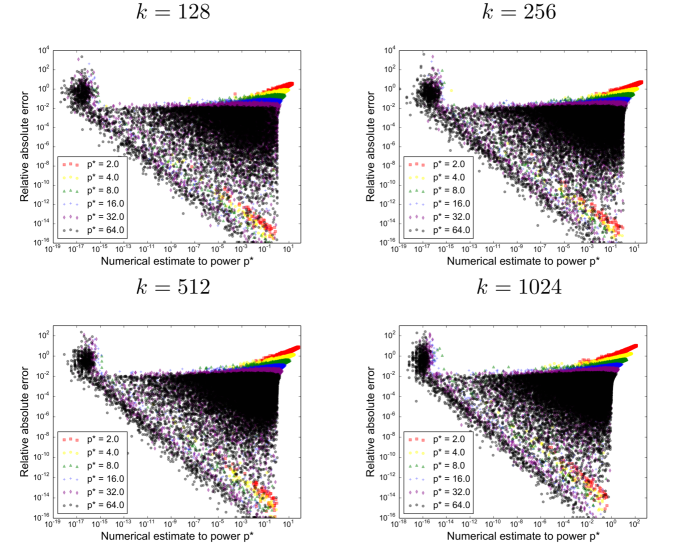
Figure 1: Empirical estimate of $\tau$ to construct a piecewise method. For each $k\in\{128,256,512,1024\}$, 32 replicate max-convolutions (on vectors filled with uniform values) are performed. Error from two sources can be seen: error due to underflow is depicted in the sharp left mode, whereas error due to imperfect approximation, where $\|\cdot\|_{p^{*}}>\|\cdot\|_{\infty}$ can be seen in the gradual mode on the right. Error due to $p^{*}$-norm approximation is significantly smaller when $p^{*}$ is larger (thereby flattening the right mode), but larger $p^{*}$ values are more susceptible to underflow, pushing more indices into the left mode. Regardless of the value of $k$, error due to underflow occurs when ${\left(\|\cdot\|_{p^{*}}\right)}^{p^{*}}$ goes below $\approx{10}^{-15}$; this is approximately the numerical tolerance for $\tau$ described by the numpy documentation. Therefore, at each index $m$ we can construct a piecewise method that uses the largest value of $p^{*}$ for which the FFT convolution result is not close to the machine precision (i.e., $({\|u^{(m)}\|}_{p^{*}})^{p^{*}}\geq\tau$ for some $\tau>{10}^{-15}$).

Because Cooley-Tukey implementations of FFT-based convolution (e.g., the numpy implementation) are widely applied to large problems with extremely small error, we will make a simplification and assume that, when constraining the FFT result to reach a value higher than machine epsilon (+ tolerance threshold), the error from the FFT is negligible in comparison to the error introduced by the $p^{*}$-norm approximation. This is firstly because the only source of numerical error during FFT (assuming an FFT implementation with numerically precise twiddle factors) on vectors in ${[0,1]}^{k}$ will be the result of underflow from repeated addition and subtraction (neglecting the non-influencing multiplication with twiddle factors, which each have magnitude $1$). The numerically imprecise routines are thus limited to $(x+y)-x$; when $x>>y$ (i.e., $\frac{y}{x}<\epsilon\approx{10}^{-15}$, the machine precision), then $(x+y)-x$ will return $0$ instead of $y$. To recover at least one bit of the significand, the intermediate results of the FFT must surpass machine precision $\epsilon$ (since the worst case addition initially happens with the maximum $x=1.0$).

The maximum sum of any values from a list of $k$ such elements can never exceed $k$; for this reason, a conservative estimate of the numerical tolerance of an FFT (with regard to underflow) will be the smallest value of $y$ for which $\frac{y}{k}>\epsilon$; thus, $y>\epsilon k$. This yields a conservative estimate of the minimum value in one index at the result of an FFT convolution: when the result at some index $m$ is $>\epsilon k$, then the result should be numerically stable. For this reason, we use a numerical tolerance $\tau={10}^{-12}$, thereby ensuring that the vast majority of numerical error for the numerical max-convolution algorithm is due to the $p^{*}$-norm approximation (i.e., employing $\|u^{(m)}\|_{p^{*}}$ instead of $\|u^{(m)}\|_{\infty}$) and not due to the long-used and numerically performant FFT result. Furthermore, in practice the mean squared error due to FFT will be much smaller than the conservative worst-case outlined here, because it is difficult for the largest intermediate summed value (in this case $x$) to be consistently large when many such very small values (in this case $y$) are encountered in the same list. Although $\tau$ could be chosen specifically for a problem of size $k$, note that this simple derivation is very conservative and thus it would be better to use a tighter bound for choosing $\tau$. Regardless, for an FFT implementation that isn’t as performant (e.g., because it uses float types instead of double), increasing $\tau$ slightly would suffice.

Therefore, from this point forward we consider that the dominant cause of error to come from the max-convolution approximation. Using larger $p^{*}$ values will provide a closer approximation; however, using a larger value of $p^{*}$ may also drive values to zero (because the inputs $L$ and $R$ will be normalized within Algorithm 1 so that the maximum of each is 1 when convolved via FFT), limiting the applicability of large $p^{*}$ to indices $m$ for which $vM[m]\geq\tau$.

Through this lens, the choice of $p^{*}$ can be characterized by two opposing sources of error: higher $p^{*}$ values better approximate $\|u^{(m)}\|_{p^{*}}$ but will be numerically unstable for many indices; lower $p^{*}$ values provide worse approximations of $\|u^{(m)}\|_{p^{*}}$ but will be numerically unstable for only few indices. These opposing sources of error pose a natural method for improving the accuracy of this max-convolution approximation. By considering a small collection of $p^{*}$ values, we can compute the full numerical estimate (at all indices) with each $p^{*}$ using Algorithm 1; computing the full result at a given $p^{*}$ is $\in O(k\log_{2}(k))$, so doing so on some small number $c$ of $p^{*}$ values considered, then the overall runtime will be $\in O(ck\log_{2}(k))$. Then, a final estimate is computed at each index by using the largest $p^{*}$ that is stable (with respect to underflow) at that index. Choosing the largest $p^{*}$ (of those that are stable with respect to underflow) corresponds to minimizing the bleed-in error, because the larger $p^{*}$ becomes, the more muted the non-maximal terms in the norm become (and thus the closer the $p^{*}$-norm becomes to the true maximum).

Here we introduce this piecewise method and compare it to the simpler low-value $p^{*}=8$ and high-value $p^{*}=64$ methods and analyze the worst-case error of the piecewise method.

Algorithm 2 Piecewise numerical max-convolution , a numerical method to estimate the max-convolution of nonnegative vectors (revised to reduce bleed-in error). This procedure uses a $p^{*}$ close to the largest possible stable value at each result index. The return value is a numerical estimate of the max-convolution $L*_{\max}R$. The runtime is in $O(k\log_{2}(k)\log_{2}(p^{*}_{\max}))$.

1:procedure numericalMaxConvolvePiecewise($L$, $R$, $p^{*}_{\max}$)

2:    $\ell_{\max}\leftarrow\operatornamewithlimits{argmax}_{\ell}L[\ell]$

3:    $r_{\max}\leftarrow\operatornamewithlimits{argmax}_{r}R[r]$

4:    $L^{\prime}\leftarrow\frac{L}{L[\ell_{\max}]}$

5:    $R^{\prime}\leftarrow\frac{R}{R[r_{\max}]}$ $\triangleright$ Scale to a proportional problem on $L^{\prime},R^{\prime}$

6:    $allPStar\leftarrow[2^{0},2^{1},\dots,2^{\big{\lceil}\log_{2}(p^{*}_{\max})\big{\rceil}}]$

7:    for $i\in\{0,1,\ldots len(allPStar)\}$ do

8:         $resForAllPStar[i]\leftarrow$ fftNonnegMaxConvolveGivenPStar($L^{\prime}$, $R^{\prime}$, $allPStar[i]$)

9:    end for

10:    for $m\in\{0,1,\ldots len(L)+len(R)-1\}$ do

11:         $maxStablePStarIndex[m]\leftarrow\max\{i:~{}{\left(resForAllPStar[i][m]\right)}^{\text{allPStar[$i$]}}\geq\tau)\}$

12:    end for

13:    for $m\in\{0,1,\ldots len(L)+len(R)-1\}$ do

14:         $i\leftarrow maxStablePStarIndex[m]$

15:         $result[m]\leftarrow resForAllPStar[i][m]$

16:    end for

17:    return $L[\ell_{\max}]\times R[r_{\max}]\times result$ $\triangleright$ Undo previous scaling

18:end procedure

3 Results

This section derives theoretical error bounds as well as a practical comparison on an example for the standard piecewise method. Furthermore the development of an improvement with affine scaling is shown. Eventually, an evaluation of the latter is performed on a larger problem. Therefore we applied our technique to compute the Viterbi path for a hidden Markov model (HMM) to assess runtime and the level of error propagation.

3.1 Error and Runtime Analysis of the Piecewise Method

We first analyze the error for a particular underflow-stable $p^{*}$ and then use that to generalize to the piecewise method, which seeks to use the highest underflow-stable $p^{*}$.

3.1.1 Error Analysis for a Fixed Underflow-Stable $p^{*}$:

We first scale $L$ and $R$ into $L^{\prime}$ and $R^{\prime}$ respectively, where the maximum elements of both $L^{\prime}$ and $R^{\prime}$ are $1$; the absolute error can be found by unscaling the absolute error of the scaled problem:

$$|exact(L,R)[m]-numeric(L^{\prime},R^{\prime})[m]|\\ =\max_{\ell}L[\ell]~{}\max_{r}R[r]\;|exact(L^{\prime},R^{\prime})[m]-numeric(L^{\prime},R^{\prime})[m]|.$$

We first derive an error bound for the scaled problem on $L^{\prime},R^{\prime}$ (any mention of a vector $u^{(m)}$ refers to the scaled problem), and then reverse the scaling to demonstrate the error bound on the original problem on $L,R$.

For any particular “underflow-stable” $p^{*}$ (i.e., any value of $p^{*}$ for which ${\left(\|u^{(m)}\|_{p^{*}}\right)}^{p^{*}}\geq\tau$), the absolute error for the numerical method for fast max-convolution can be bound fairly easily by factoring out the maximum element of $u^{(m)}$ (this maximum element is equivalent to the Chebyshev norm) from the $p^{*}$-norm:

$$|exact(L^{\prime},R^{\prime})[m]-numeric(L^{\prime},R^{\prime})[m]|$$

$$= |\|u^{(m)}\|_{p^{*}}-\|u^{(m)}\|_{\infty}|$$

$$= \|u^{(m)}\|_{p^{*}}-\|u^{(m)}\|_{\infty}$$

$$= \|u^{(m)}\|_{\infty}\left(\frac{\|u^{(m)}\|_{p^{*}}}{\|u^{(m)}\|_{\infty}}-1\right)$$

$$= \|u^{(m)}\|_{\infty}\left(\|\frac{u^{(m)}}{\|u^{(m)}\|_{\infty}}\|_{p^{*}}-1\right)$$

$$= \|u^{(m)}\|_{\infty}\left(\|v^{(m)}\|_{p^{*}}-1\right)$$

where $v^{(m)}$ is a nonnegative vector of the same length as $u^{(m)}$ (this length is denoted $k_{m}$) where $v^{(m)}$ contains one element equal to $1$ (because the maximum element of $u^{(m)}$ must, by definition, be contained within $u^{(m)}$) and where no element of $v^{(m)}$ is greater than 1 (also provided by the definition of the maximum).

$$\|v^{(m)}\|_{p^{*}} \leq \|(1,1,\ldots 1)\|_{p^{*}}$$

$$= {\left(\sum_{i}^{k_{m}}1^{p^{*}}\right)}^{\frac{1}{p^{*}}}$$

$$= {k_{m}}^{\frac{1}{p^{*}}}$$

Thus, since $\|v^{(m)}\|_{p^{*}}\geq 1$, the error is bound:

$$|exact(L^{\prime},R^{\prime})[m]-numeric(L^{\prime},R^{\prime})[m]$$

$$= \|u^{(m)}\|_{\infty}\left(\|v^{(m)}\|_{p^{*}}-1\right)$$

$$\leq \|v^{(m)}\|_{p^{*}}-1$$

$$\leq k_{m}^{\frac{1}{p^{*}}}-1,$$

because $\forall m,~{}\|u^{(m)}\|_{\infty}\leq 1$ for a scaled problem on $L^{\prime},R^{\prime}$.

3.1.2 Error Analysis of Piecewise Method

However, the bounds derived above are only applicable for $p^{*}$ where $\|u^{(m)}\|_{p^{*}}^{p^{*}}\geq\tau$. The piecewise method is slightly more complicated, and can be partitioned into two cases: In the first case, the top contour is used (i.e., when $p^{*}_{\max}$ is underflow-stable). Conversely, in the second case, a middle contour is used (i.e., when $p^{*}_{\max}$ is not underflow-stable). In this context, in general a contour comprises of a set of indices $m$ with the same maximum stable $p^{*}$.

In the first case, when we use the top contour $p^{*}=p^{*}_{\max}$, we know that $p^{*}_{\max}$ must be underflow-stable, and thus we can reuse the bound given an underflow-stable $p^{*}$.

In the second case, because the $p^{*}$ used is $<p^{*}_{\max}$, it follows that the next higher contour (using $2p^{*}$) must not be underflow-stable (because the highest underflow-stable $p^{*}$ is used and because the $p^{*}$ are searched in log-space). The bound derived above that demonstrated

$$\|u^{(m)}\|_{p^{*}}\leq\|u^{(m)}\|_{\infty}k_{m}^{\frac{1}{p^{*}}}$$

can be combined with the property that $\|\cdot\|_{p^{*}}\geq\|\cdot\|_{\infty}$ for any $p^{*}\geq 1$ to show that

$$\|u^{(m)}\|_{\infty}\in\left[\frac{\|u^{(m)}\|_{p^{*}}}{k_{m}^{\frac{1}{p^{*}}}},\|u^{(m)}\|_{p^{*}}\right].$$

Thus the absolute error can be bound again using the fact that we are in a middle contour:

$$= \|u^{(m)}\|_{p^{*}}-\|u^{(m)}\|_{\infty}$$

$$= \|u^{(m)}\|_{p^{*}}\left(1-\frac{\|u^{(m)}\|_{\infty}}{\|u^{(m)}\|_{p^{*}}}\right)$$

$$\leq \|u^{(m)}\|_{p^{*}}\left(1-k_{m}^{\frac{-1}{p^{*}}}\right)$$

$$< \tau^{\frac{1}{2p^{*}}}\left(1-k_{m}^{\frac{-1}{p^{*}}}\right).$$

The absolute error from middle contours will be quite small when $p^{*}=1$ is the maximum underflow-stable value of $p^{*}$ at index $m$, because $\tau^{\frac{1}{2p^{*}}}$, the first factor in the error bound, will become $\sqrt{\tau}\approx 10^{-6}$, and $1-k_{m}^{\frac{-1}{p^{*}}}<1$ (qualitatively, this indicates that a small $p^{*}$ is only used when the result is very close to zero, leaving little room for absolute error). Likewise, when a very large $p^{*}$ is used, then $1-k_{m}^{\frac{-1}{p^{*}}}$ becomes very small, while $\tau^{\frac{1}{2p^{*}}}<1$ (qualitatively, this indicates that when a large $p^{*}$ is used, the $\|\cdot\|_{p^{*}}\approx\|\cdot\|_{\infty}$, and thus there is little absolute error). Thus for the extreme values of $p^{*}$, middle contours will produce fairly small absolute errors. The unique mode $p^{*}_{mode}$ can be found by finding the value that solves

$$\frac{\partial}{\partial p^{*}_{mode}}~{}\left(\tau^{\frac{1}{2p^{*}_{mode}}}\left(1-k_{m}^{\frac{-1}{p^{*}_{mode}}}\right)\right)=0,$$

which yields

$$p^{*}_{mode}=\frac{\log_{2}(k_{m})}{\log_{2}(-\frac{2\log_{2}(k)-\log_{2}(\tau)}{\log_{2}(\tau)})}.$$

An appropriate choice of $p^{*}_{\max}$ should be $>p^{*}_{mode}$ so that the error for any contour (both middle contours and the top contour) is smaller than the error achieved at $p^{*}_{mode}$, allowing us to use a single bound for both. Choosing $p^{*}_{\max}=p^{*}_{mode}$ would guarantee that all contours are no worse than the middle-contour error at $p^{*}_{mode}$; however, using $p^{*}_{\max}=p^{*}_{mode}$ is still quite liberal, because it would mean that for indices in the highest contour (there must be a nonempty set of such indices, because the scaling on $L^{\prime}$ and $R^{\prime}$ guarantees that the maximum index will have an exact value of $1$, meaning that the approximation endures no underflow and is underflow-stable for every $p^{*}$), a better error could be achieved by increasing $p^{*}_{\max}$. For this reason, we choose $p^{*}_{\max}$ so that the top-contour error produced at $p^{*}_{\max}$ is not substantially larger than all errors produced for $p^{*}$ before the mode (i.e., for $p^{*}<p^{*}_{mode}$).

Choosing any value of $p^{*}_{\max}>p^{*}_{mode}$ guarantees the worst-case absolute error bound derived here; however, increasing $p^{*}_{\max}$ further over $p^{*}_{mode}$ may possibly improve the mean squared error in practice (because it is possible that many indices in the result would be numerically stable with $p^{*}$ values substantially larger than $p^{*}_{mode}$). However, increasing $p^{*}_{\max}>>p^{*}_{mode}$ will produce diminishing returns and generally benefit only a very small number of indices in the result, which have exact values very close to $1$. In order to balance these two aims (increasing $p^{*}_{\max}$ enough over $p^{*}_{mode}$ but not excessively so), we make a qualitative assumption that a non-trivial number of indices require us to use a $p^{*}$ below $p^{*}_{mode}$; therefore, increasing $p^{*}_{\max}$ to produce an error significantly smaller than the lowest worst-case error for contours below the mode (i.e. $p^{*}<p^{*}_{mode}$) will increase the runtime without significantly decreasing the mean squared error (which will become dominated by the errors from indices that use $p^{*}<p^{*}_{mode}$). The lowest worst-case error contour below the mode is $p^{*}=1$ (because the absolute error function is unimodal, and thus must be increasing until $p^{*}_{mode}$ and decreasing afterward); therefore, we heuristically specify that $p^{*}_{\max}$ should produce a worst-case error on a similar order of magnitude to the worst-case error produced with $p^{*}=1$. In practice, specifying the errors at $p^{*}_{\max}$ and $p^{*}=1$ should be equal is very conservative (it produces very large estimates of $p^{*}_{\max}$, which sometimes benefit only one or two indices in the result); for this reason, we heuristically choose that the worst-case error at $p^{*}_{\max}$ should be no worse than square root of the worst case error at $p^{*}=1$ (this makes the choice of $p^{*}_{\max}$ less conservative because the errors at $p^{*}=1$ are very close to zero, and thus their square root is larger). The square root was chosen because it produced, for the applications described in this paper, the smallest value of $p^{*}_{\max}$ for which the mean squared error was significantly lower than using $p^{*}_{\max}=p^{*}_{mode}$ (the lowest value of $p^{*}_{\max}$ guaranteed to produce the absolute error bound). This heuristic does satisfy the worst-case bound outlined here (because, again, $p^{*}_{\max}>p^{*}_{mode}$), but it could be substantially improved if an expected distribution of magnitudes in the result vector were known ahead of time: prior knowledge regarding the number of points stable at each $p^{*}$ considered would enable a well-motivated choice of $p^{*}_{\max}$ that truly optimizes the expected mean squared error.

From this heuristic choice of $p^{*}_{\max}$, solving

$$\sqrt{\sqrt{\tau}\left(1-\frac{1}{k}\right)}=k^{\frac{1}{p^{*}_{\max}}}-1$$

(with the square root of the worst-case at $p^{*}=1$ on the left and the worst-case error at $p^{*}_{\max}$ on the right) yields

$$p^{*}_{\max} = \frac{\log_{2}(k)}{\log_{2}(1+\sqrt{\sqrt{\tau}\left(1-\frac{1}{k}\right)})}$$

$$\approx \frac{\log_{2}(k)}{\log_{2}(1+\sqrt{\sqrt{\tau}})}$$

for any non-trivial problem (i.e., when $k>>1$), and thus

$$p^{*}_{\max}\approx\log_{1+\tau^{\frac{1}{4}}}(k),$$

indicating that the absolute error at the top contour will be roughly equal to the fourth root of $\tau$.

3.1.3 Worst-case Absolute Error

By setting $p^{*}_{\max}$ in this manner, we guarantee that the absolute error at any index of any unscaled problem on $L,R$ is less than

$$\max_{\ell}L[\ell]~{}\max_{r}R[r]~{}\tau^{\frac{1}{2p^{*}_{mode}}}\left(1-k_{m}^{\frac{-1}{p^{*}_{mode}}}\right)$$

where $p^{*}_{mode}$ is defined above. The full formula for the middle-contour error at this value of $p^{*}_{mode}$ does not simplify and is therefore quite large; for this reason, it is not reported here, but this gives a numeric bound of the worst case middle-contour error that is bound in terms of the variable $k$ (and with no other free variables).

3.1.4 Runtime Analysis

The piecewise method clearly performs $\log_{2}(p^{*}_{\max})$ FFTs (each requiring $O(k\log_{2}(k))$ steps); therefore, since $p^{*}_{\max}$ is chosen to be $\log_{1+\tau^{\frac{1}{4}}}(k)$ (to achieve the desired error bound), the total runtime is thus

$$O(k\log_{2}(k)\log_{2}(\log_{1+\tau^{\frac{1}{4}}}(k)).$$

For any practically sized problem, the $\log_{2}(\log_{1+\tau^{\frac{1}{4}}}(k))$ factor is essentially a constant; even when $k$ is chosen to be the number of particles in the observable universe ($\approx 2^{270}$; Eddington, 1923), the $\log_{2}(\log_{1+\tau^{\frac{1}{4}}}(k))$ is $\approx 18$, meaning that for any problem of practical size, the full piecewise method is no more expensive than computing between $1$ and $18$ FFTs.

3.2 Comparison of Low-Value $p^{*}=8$, High-value $p^{*}=64$, and Piecewise Method

We first use an example max-convolution problem to compare the results from the low-value $p^{*}=8$, the high-value $p^{*}=64$ and piecewise methods. At every index, these various approximation results are compared to the exact values, as computed by the naive quadratic method (Figure 2(a)).

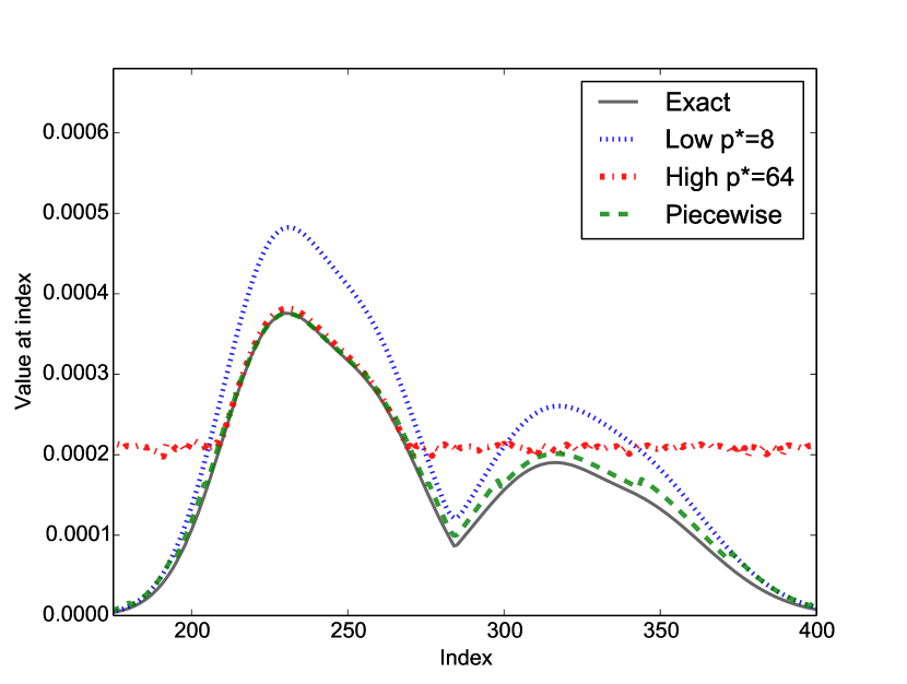
(a)

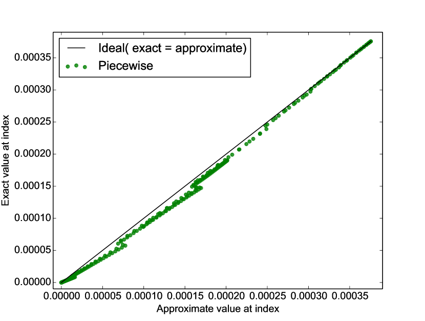
(b)

Figure 2: The accuracy of numerical fast max-convolution methods. (a) Different approximations for a sample max-convolution problem. The low-$p^{*}$ method is underflow-stable, but overestimates the result. The high-$p^{*}$ method is accurate when underflow-stable, but experiences underflow at many indices. The piecewise method stitches together approximations from different $p^{*}$ to maintain underflow-stability. (b) Exact vs. piecewise approximation at various indices of the same problem. A clear banding pattern is observed with one tight, elliptical cluster for each contour. The slope of the clusters deviates more for the contours using lower $p^{*}$ values.

3.3 Improved Affine Piecewise Method

Figure 2(b) depicts a scatter plot of the exact result vs. the piecewise approximation at every index (using the same problem from Figure 2(a)). It shows a clear banding pattern: the exact and approximate results are clearly correlated, but each contour (i.e., each collection of indices that use a specific $p^{*}$) has a different average slope between the exact and approximate values, with higher $p^{*}$ contours showing a generally larger slope and smaller $p^{*}$ contours showing greater spread and lower slopes. This intuitively makes sense, because the bounds on $\|u^{(m)}\|_{\infty}\in[\|u^{(m)}\|_{p^{*}}k_{m}^{\frac{-1}{p^{*}}},\|u^{(m)}\|_{p^{*}}]$ derived above constrain the scatter plot points inside a quadrilateral envelope (Figure 3).

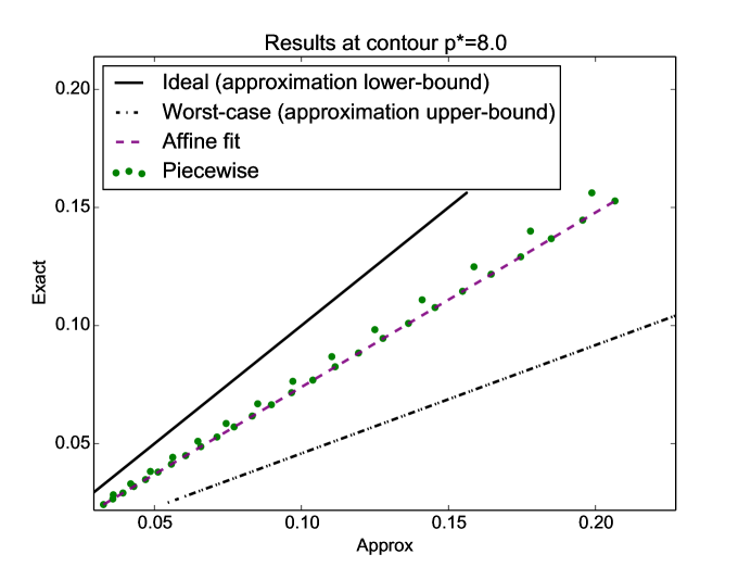
Figure 3: A single contour from the piecewise approximation. The cluster of points (one point for each index in the previous figure) is bounded by the exact value (ideal approximation) and the approximation upper-bound for $p^{*}=8$ (worst-case approximation). The points are well described by an affine function fit using the left-most and right-most points.

The correlations within each contour can be exploited to correct biases that emerge for smaller $p^{*}$ values. In order to do this, $\|u^{(m)}\|_{\infty}$ must be computed for at least two points $m_{1}$ and $m_{2}$ within the contour, so that a mapping $\|u^{(m)}\|_{p^{*}}\approx f(\|u^{(m)}\|_{p^{*}})=a\|u^{(m)}\|_{p^{*}}+b$ can be constructed. Fortunately, a single $\|u^{(m)}\|_{\infty}$ can be computed exactly in $O(k)$ (by actually computing a single $u^{(m)}$ and computing its max, which is equivalent to computing a single index result via the naive quadratic method). As long as the exact value $\|u^{(m)}\|_{\infty}$ is computed for only a small number of indices, the order of the runtime will not change (each contour already costs $O(k\log_{2}(k))$, so adding a small number of $O(k)$ steps for each contour will not change the asymptotic runtime).

If the two indices chosen are

$$m_{\min}=\operatornamewithlimits{argmin}_{m\in contour(p^{*})}\|u^{(m)}\|_{p^{*}}$$

$$m_{\max}=\operatornamewithlimits{argmax}_{m\in contour(p^{*})}\|u^{(m)}\|_{p^{*}},$$

then we are guaranteed that the affine function $f$ can be written as a convex combination of the exact values at those extreme points (using barycentric coordinates):

$$f(\|u^{(m)}\|_{p^{*}})=\lambda_{m}\|u^{(m_{\max})}\|_{\infty}+\left(1-\lambda_{m}\right)\|u^{(m_{\min})}\|_{\infty}$$

$$\lambda_{m}=\frac{\|u^{(m)}\|_{p^{*}}-\|u^{(m_{\min})}\|_{p^{*}}}{\|u^{(m_{\max})}\|_{p^{*}}-\|u^{(m_{\min})}\|_{p^{*}}}\in[0,1]$$

Thus, by computing $\|u^{(m_{\min})}\|_{\infty}$ and $\|u^{(m_{\max})}\|_{\infty}$ (each in $O(k)$ steps), we can compute an affine function $f$ to correct contour-specific trends (Algorithm 3).

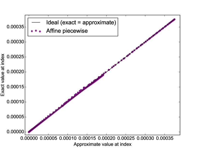
(a)

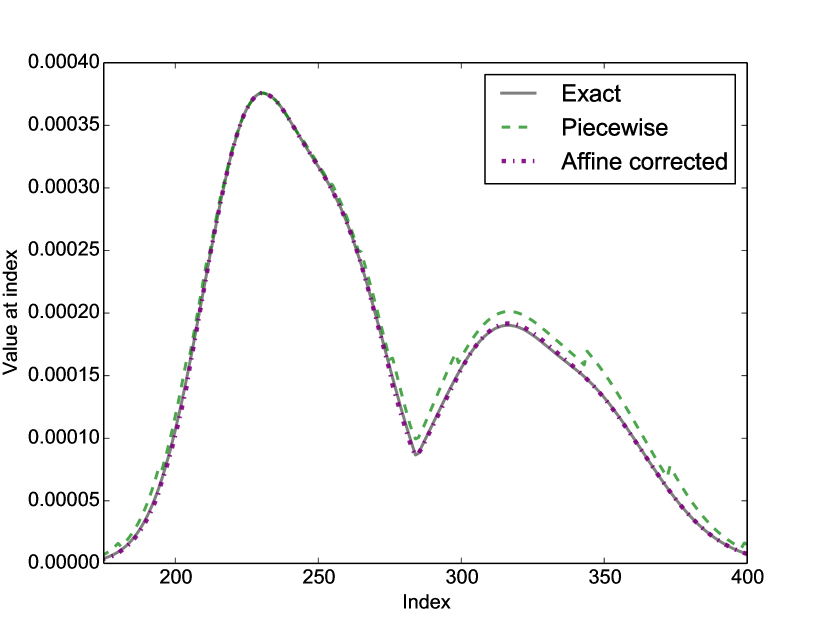
(b)

Figure 4: Piecewise method with affine contour fitting. The approximate values at each index of the max-convolution problem are almost identical to the exact result at the same index.

Algorithm 3 Improved affine piecewise numerical max-convolution, a numerical method to estimate the max-convolution nonnegative vectors (further revised to reduce numerical error). This procedure uses a $p^{*}$ close to the largest possible stable value at each result index. The return value is a numerical estimate of the max-convolution $L*_{\max}R$. The runtime is in $O(k\log_{2}(k)\log_{2}(p^{*}_{\max}))$.

1:procedure numericalMaxConvolvePiecewiseAffine($L$, $R$, $p^{*}_{\max}$)

2:    $\ell_{\max}\leftarrow\operatornamewithlimits{argmax}_{\ell}L[\ell]$

3:    $r_{\max}\leftarrow\operatornamewithlimits{argmax}_{r}R[r]$

4:    $L^{\prime}\leftarrow\frac{L}{L[\ell_{\max}]}$

5:    $R^{\prime}\leftarrow\frac{R}{R[r_{\max}]}$ $\triangleright$ Scale to a proportional problem on $L^{\prime},R^{\prime}$

6:    $allPStar\leftarrow[2^{0},2^{1},\dots,2^{\big{\lceil}\log_{2}(p^{*}_{\max})\big{\rceil}}]$

7:    for $i\in\{0,1,\ldots len(allPStar)\}$ do

8:         $resForAllPStar[i]\leftarrow$ fftNonnegMaxConvolveGivenPStar($L^{\prime}$, $R^{\prime}$, $allPStar[i]$)

9:    end for

10:    for $m\in\{0,1,\ldots len(L)+len(R)-1\}$ do

11:         $maxStablePStarIndex[m]\leftarrow\max\{i:~{}{\left(resForAllPStar[i][m]\right)}^{\text{allPStar[$i$]}}\geq\tau)\}$

12:    end for

13:    $result\leftarrow$affineCorrect$(resForAllPStar,maxStablePStarIndex)$

14:    return $L[\ell_{\max}]\times R[r_{\max}]\times result$ $\triangleright$ Undo previous scaling

15:end procedure

Algorithm 4 Subroutine for correcting errors in a contour, with an affine transformation based on exact boundary points. It needs the results of the evaluation of the different $p$-norms as well as the (index of the) maximum stable values of $p^{*}$ at every index.

1:procedure affineCorrect($resForAllPStar$, $maxStablePStarIndex$)

2:    $\forall i,slope[i]\leftarrow 1$

3:    $\forall i,bias[i]\leftarrow 0$

4:    $usedPStar\leftarrow set(maxStablePStarIndex)$

5:    for $i\in usedPStar$ do

6:         $contour\leftarrow\{m:maxStablePStarIndex[m]=i\}$

7:         $mMin\leftarrow argmin_{m\in contour}resForAllPStar[i][m]$

8:         $mMax\leftarrow argmax_{m\in contour}resForAllPStar[i][m]$

9:         $xMin\leftarrow resForAllPStar[i][mMin]$

10:         $xMax\leftarrow resForAllPStar[i][mMax]$

11:         $yMin\leftarrow\texttt{maxConvolutionAtIndex}(mMin)$

12:         $yMax\leftarrow\texttt{maxConvolutionAtIndex}(mMax)$

13:         if $xMax>xMin$ then

14:             $slope[i]\leftarrow\frac{yMax-yMin}{xMax-xMin}$

15:             $bias[i]\leftarrow yMin-slope[i]\times xMin$

16:         else

17:             $slope[i]\leftarrow\frac{yMax}{xMax}$

18:         end if

19:    end for

20:    for $m\in\{0,1,\ldots len(L)+len(R)-1\}$ do

21:         $i\leftarrow maxStablePStarIndex[m]$

22:         $result[m]\leftarrow resForAllPStar[i][m]\times slope[i]+bias[i]$

23:    end for

24:    return $result$

25:end procedure

3.3.1 Error Analysis of Improved Affine Piecewise Method

By exploiting the convex combination used to define $f$, the absolute error of the affine piecewise method can also be bound. Qualitatively, this is because, by fitting on the extrema in the contour, we are now interpolating. If the two points used to determine the parameters of the affine function were not chosen in this manner to fit the affine function, then it would be possible to choose two points with very close x-values (i.e., similar approximate values) and disparate y-values (i.e., different exact values), and extrapolating to other points could propagate a large slope over a large distance; using the extreme points forces the affine function to be a convex combination of the extrema, thereby avoiding this problem.

$$f(\|u^{(m)}\|_{p^{*}})=\lambda_{m}\|u^{(m_{\max})}\|_{\infty}+\left(1-\lambda_{m}\right)\|u^{(m_{\min})}\|_{\infty}\\ \in\left[\lambda_{m}\frac{\|u^{(m_{\max})}\|_{p^{*}}}{k_{m_{\max}}^{\frac{1}{p^{*}}}}+\left(1-\lambda_{m}\right)\frac{\|u^{(m_{\min})}\|_{p^{*}}}{k_{m_{\min}}^{\frac{1}{p^{*}}}},\right.\\ \left.\lambda_{m}\|u^{(m_{\max})}\|_{p^{*}}+\left(1-\lambda_{m}\right)\|u^{(m_{\min})}\|_{p^{*}}\right]\\ \subseteq\left[\lambda_{m}\frac{\|u^{(m_{\max})}\|_{p^{*}}}{k^{\frac{1}{p^{*}}}}+\left(1-\lambda_{m}\right)\frac{\|u^{(m_{\min})}\|_{p^{*}}}{k^{\frac{1}{p^{*}}}},\right.\\ \left.\lambda_{m}\|u^{(m_{\max})}\|_{p^{*}}+\left(1-\lambda_{m}\right)\|u^{(m_{\min})}\|_{p^{*}}\right]\\ =\left[k^{\frac{-1}{p^{*}}}\left(\lambda_{m}\|u^{(m_{\max})}\|_{p^{*}}+\left(1-\lambda_{m}\right)\|u^{(m_{\min})}\|_{p^{*}}\right),\right.\\ \left.\lambda_{m}\|u^{(m_{\max})}\|_{p^{*}}+\left(1-\lambda_{m}\right)\|u^{(m_{\min})}\|_{p^{*}}\right]\\ =\left[k^{\frac{-1}{p^{*}}}\|u^{(m)}\|_{p^{*}},\|u^{(m)}\|_{p^{*}}\right]$$

The worst-case absolute error of the scaled problem on $L^{\prime},R^{\prime}$ can be defined

$$\max_{m}|~{}f(\|u^{(m)}\|_{p^{*}})-\|u^{(m)}\|_{\infty}~{}|.$$

Because the function $f(\|u^{(m)}\|_{p^{*}})-\|u^{(m)}\|_{\infty}$ is affine, it’s derivative can never be zero, and thus Lagrangian theory states that the maximum must occur at a boundary point. Therefore, the worst-case absolute error is

$$\leq \max\{\|u^{(m)}\|_{p^{*}}-\|u^{(m)}\|_{\infty},\|u^{(m)}\|_{\infty}-\|u^{(m)}\|_{p^{*}}k^{\frac{-1}{p^{*}}}\}$$

$$= \|u^{(m)}\|_{p^{*}}-\|u^{(m)}\|_{\infty},$$

which is identical to the worst-case error bound before applying the affine transformation $f$. Thus applying the affine transformation can dramatically improve error, but will not make it worse than the original worst-case.

3.4 Demonstration on Hidden Markov Model With Toeplitz Transition Matrix

One example that profits from fast max-convolution of non-negative vectors is computing the Viterbi path using a hidden Markov model (HMM) (i.e., the maximum a posteriori states) with an additive transition function satisfying $\Pr(X_{i+1}=a|X_{i}=b)\propto\delta(a-b)$ for some arbitrary function $\delta$ ($\delta$ can be represented as a table, because we are considering all possible discrete functions). This additivity constraint is equivalent to the transition matrix being a “Toeplitz matrix”: the transition matrix $T_{a,b}=\Pr(X_{i+1}=a|X_{i}=b)$ is a Toeplitz matrix when all cells diagonal from each other (to the upper left and lower right) have identical values (i.e., $\forall a,\forall b,~{}T_{a,b}=T_{a+1,b+1}$). Because of the Markov property of the chain, we only need to max-marginalize out the latent variable at time $i$ to compute the distribution for the next latent variable $X_{i+1}$ and all observed values of the data variables $D_{0}\dots D_{i+1}$. This procedure, called the Viterbi algorithm, is continued inductively:

$$\max_{x_{0},x_{1},\ldots x_{i-1}}\Pr(D_{0},D_{1},\ldots D_{i-1},X_{0}=x_{0},X_{1}=x_{1},\ldots,X_{i}=x_{i})=\\ \\ \max_{x_{i-1}}\max_{x_{0},x_{1},\dots x_{i-2}}~{}\Pr(D_{0},D_{1},\ldots D_{i-2},X_{0}=x_{0},X_{1}=x_{1},\ldots,X_{i-1}=x_{i-1})\\ \Pr(D_{i-1}|X_{i-1}=x_{i-1})\Pr(X_{i}=x_{i}|X_{i-1}=x_{i-1})\\$$

and continuing by exploiting the self-similarity on a smaller problem to proceed inductively, revealing a max-convolution (for this specialized HMM with additive transitions):

$$=\max_{x_{i-1}}~{}fromLeft[i-1]\Pr(D_{i-1}|X_{i-1}=x_{i-1})\delta[x_{i}-x_{i-1}]=\\ \left(fromLeft[i-1]~{}likelihood[D_{i-1}]\right)~{}*_{\max}~{}\delta[x_{i}-x_{i-1}].\\$$

After computing this left-to-right pass (which consisted of $n-1$ max-convolutions and vector multiplications), we can find the maximum a posteriori configuration of the latent variables $X_{0},\ldots X_{n-1}=x_{0}^{*},\ldots x_{n-1}^{*}$ backtracking right-to-left, which can be done by finding the variable value $x_{i}$ that maximizes $fromLeft[i][x_{i}]\times\delta[x_{i+1}^{*}-x_{i}]$ (thus defining $x_{i}^{*}$ and enabling induction on the right-to-left pass). The right-to-left pass thus requires $O(nk)$ steps (Algorithm 5). Note that the full max-marginal distributions on each latent variable $X_{i}$ can be computed via a small modification, which would perform a more complex right-to-left pass that is nearly identical to the left-to-right pass, but which performs subtraction instead of addition (i.e., by reversing the vector representation of the PMF of the subtracted argument before it is max-convolved; Serang, 2014).

Algorithm 5 Viterbi for models with additive transitions, which accepts the length $k$ vector $prior$, a list of $n$ binned observations $data$, a $a\times k$ matrix of likelihoods (where $a$ is the number of bins used to discretize the data) $likelihoods$, and a length $2k-1$ vector $\delta$ that describes the transition probabilities. The algorithm returns a Viterbi path of length $n$, where each element in the path is a valid state $\in\{0,1,\ldots k-1\}$.

1:procedure ViterbiForAdditiveTransitions($prior,data,likelihood,\delta$)

2:    $fromLeft[0]\leftarrow prior$

3:    for $i=0$ to $n-2$ do

4:         $fromLeft[i]\leftarrow fromLeft[i]\times likelihood[data[i]]$

5:         $fromLeft[i+1]\leftarrow fromLeft[i]*_{\max}\delta$

6:    end for

7:    $fromLeft[n]\leftarrow fromLeft[n]\times likelihood[data[n]]$

8:    

9:    $path[n-1]\leftarrow\operatornamewithlimits{argmax}_{j}fromLeft[n-1][j]$

10:    for $i=n-2$ to $0$ do

11:         $maxProdPosterior\leftarrow-1$

12:         $argmaxProdPosterior\leftarrow-1$

13:         for $l=k$ to $1$ do

14:             $currProdPosterior\leftarrow fromLeft[i]\times\delta[l-path[i+1]]$

15:             if $currProdPosterior>maxProdPosterior$ then

16:                 $maxProdPosterior\leftarrow currProdPosterior$

17:                 $argmaxProdPosterior\leftarrow l$

18:             end if

19:         end for

20:         $path[i]\leftarrow argmaxProdPosterior$

21:    end for

22:    return $path$

23:end procedure

We apply this HMM with additive transition probabilities to a data analysis problem from economics. It is known for example, that the current figures of unemployment in a country have (among others) impact on prices of commodities like oil. If one could predict unemployment figures before the usual weekly or monthly release by the responsible government bureaus, this would lead to an information advantage and an opportunity for short-term arbitrage. The close relation of economic indicators like market prices and stock market indices (especially of indices combining several stocks of different industries) to unemployment statistics can be used to tackle this problem.

In the following demonstration of our method, we create a simple HMM with additive transitions and use it to infer the maximum a posteriori unemployment statistics given past history (i.e. how often unemployment is low and high, as well as how often unemployment goes down or up in a short amount of time) and current stock market prices (the observed data). We discretized random variables for the observed data (S&P 500, adjusted closing prices ; retrieved from YAHOO! historical stock prices: http://data.bls.gov/cgi-bin/surveymost?blsseriesCUUR0000SA0), and ”latent” variables (unemployment insurance claims, seasonally adjusted, were retrieved from the U.S. Department of Labor: https://www.oui.doleta.gov/unemploy/claims.asp). Stock prices were additionally inflation adjusted by (i.e. divided by) the consumer price index (CPI) (retrieved from the U.S. Bureau of Labor Statistics: https://finance.yahoo.com/q?s=^GSPC). The intersection of both ”latent” and observed data was available weekly from week 4 in 1967 to week 52 in 2014, resulting in 2500 data points for each type of variable.

To investigate the influence of overfitting, we partition the data in two parts, before June 2005 and after June 2005, so that we are effectively training on $\frac{2000\times 100}{2500}=80\%$ of the data points, and then demonstrate the Viterbi path on the entirety of the data (both the $80\%$ training data and the $20\%$ of the data withheld from empirical parameter estimation). Unemployment insurance claims were discretized into $512$ and stock prices were discretized into $128$ bins. Simple empirical models of the prior distribution for unemployment, the likelihood of unemployment given stock prices, and the transition probability of unemployment were built as follows: The initial or prior distribution for unemployment claims at $i=0$ was calculated by marginalizing the time series of training data for the claims (i.e. counting the number of times any particular unemployment value was reached over all possible bins). Our transition function (the conditional probability $\Pr(X_{i+1}|X_{i})$) similarly counts the number of times each possible change $X_{i+1}-X_{i}\in\{-511,-510,\ldots 511\}$ occurred over all available time points. Interestingly, the resulting transition distribution roughly resembles a Gaussian (but is not an exact Gaussian). This underscores a great quality of working with discrete distributions: while continuous distributions may have closed-forms for max-convolution (which can be computed quickly), discrete distributions have the distinct advantage that they can accurately approximate any smooth distribution. Lastly, the likelihoods of observing a stock price given the unemployment at the same time were trained using an empirical joint distribution (essentially a heatmap), which is displayed in Figure 5.

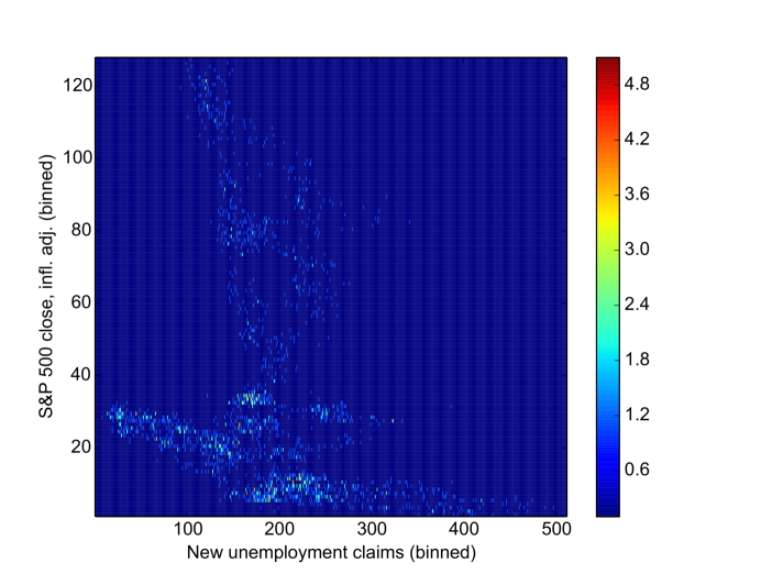
Figure 5: Heatmap for trained likelihood matrix. This heatmap depicts a joint empirical distribution between the S&P 500 index and new unemployment claims, which share a tenuous inverse relationship. Given $D_{i}$, the discretized stock index value at time $i$, row $D_{i}$ contains the likelihood table $\Pr(D_{i}|X_{i})$, which is denoted $likelihood[data[i]]$ in the code.

We compute the Viterbi path two times: First we use naive, exact max-convolution, which requires a total of $O(nk^{2})$ steps. Second, we use fast numerical max-convolution, which requires $O(n~{}k\log(k)\log(\log(k))$ steps. Despite the simplicity of the model, the exact Viterbi path (computed via exact max-convolution) is highly informative for predicting the value of unemployment, even for the $20\%$ of the data that were not used to estimate the empirical prior, likelihood, and transition distributions. Also, the numerical max-convolution method is nearly identical to the exact max-convolution method at every index (Figure 6). Even with a fairly rough discretization (i.e., $k=512$), the fast numerical method used $141.4$ seconds compared to the $292.3$ seconds required by the naive approach. This speedup will increase dramatically as $k$ is increased, because the $\log(\log(k))$ term in the runtime of the numerical max-convolution method is essentially bounded above $\log(\log(k))\leq 18$.

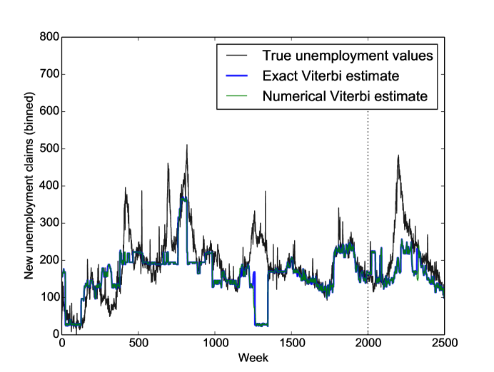
Figure 6: Viterbi analysis of employment given stock index values. The Viterbi path corresponding to the maximum a posteriori prediction of the number of new unemployment insurance claims is produced for a model where the state transition probabilities are additive. The exact Viterbi estimate tracks well with the true unemployment values. Training parameters were taken from only the true unemployment data to the left of the vertical dotted line; however, the Viterbi paths to the right of the dotted line (where unemployment data were withheld from the likelihood, prior, and transition parameters) also track well with the true unemployment statistics. The Viterbi path computed with fast numerical max-convolution (via the affine piecewise approach) is nearly identical to the result computed with the slower exact approach.

3.5 An Improved Approximation of the Chebyshev Norm

Although the $p^{*}$-norm provides a good approximation of the Chebyshev norm, it discards significant information; specifically the curve $\|u^{(m)}\|_{p^{*}}$ for various ${p^{*}}$ could be used to identify and correct the worst-case scenario where $\frac{u^{(m)}}{\|u^{(m)}\|_{\infty}}=(1,1,\ldots 1)$; using only two points, the exact value of $\|u^{(m)}\|_{\infty}$ can be computed for those worst-case $u^{(m)}$ vectors by computing the norms at two different $p^{*}$ values and solving the following equations for $\beta_{1}$:

$$\|u^{(m)}\|_{p^{*}_{1}}^{p^{*}_{1}} \propto \beta_{1}^{p^{*}_{1}}$$

$$\|u^{(m)}\|_{p^{*}_{2}}^{p^{*}_{2}} \propto \beta_{1}^{p^{*}_{2}},$$

where the proportionality constant is $k_{m}=len(u^{(m)})$ and where the computed value $\beta_{1}$ yields the exact Chebyshev norm $\|u^{(m)}\|_{\infty}$.

3.5.1 A Projection-Based Method for Estimating $\|u^{(m)}\|_{\infty}$

More generally, when there are $e_{m}\leq k_{m}$ unique values ($\beta_{i}$) in $u^{(m)}$, we can model the norms perfectly with

$$\|u^{(m)}\|_{p^{*}}^{p^{*}}=\sum_{i}^{e_{m}}h_{i}\beta_{i}^{p^{*}}$$

where $h_{i}$ is an integer that indicates the number of times $\beta_{i}$ occurs in $u^{(m)}$ (and where $\sum_{i}h_{i}=k_{m}=len(u^{(m)})$). This multi-set view of the vector $u^{(m)}$ can be used to project it down to a dimension $r$:

$$\left[\begin{array}[]{cccc}\alpha_{1}^{p^{*}}&\alpha_{2}^{p^{*}}&&\alpha_{r}^{p^{*}}\\ \alpha_{1}^{2{p^{*}}}&\alpha_{2}^{2{p^{*}}}&\cdots&\alpha_{r}^{2{p^{*}}}\\ \alpha_{1}^{3{p^{*}}}&\alpha_{2}^{3{p^{*}}}&&\alpha_{r}^{3{p^{*}}}\\ \vdots&\vdots&&\vdots\\ \alpha_{1}^{\ell{p^{*}}}&\alpha_{2}^{\ell{p^{*}}}&&\alpha_{r}^{\ell{p^{*}}}\\ \end{array}\right]\cdot\left[\begin{array}[]{c}n_{1}\\ n_{2}\\ n_{3}\\ \vdots\\ n_{r}\\ \end{array}\right]=\left[\begin{array}[]{c}\|u^{(m)}\|_{p^{*}}^{p^{*}}\\ \|u^{(m)}\|_{2{p^{*}}}^{2{p^{*}}}\\ \|u^{(m)}\|_{2{p^{*}}}^{2{p^{*}}}\\ \vdots\\ \|u^{(m)}\|_{\ell{p^{*}}}^{\ell{p^{*}}}\\ \end{array}\right].$$

By solving the above system of equations for all $\alpha_{i}$, the maximum $\hat{\alpha}=\max_{i}\alpha_{i}$ can be used to approximate the true maximum $\max_{i}\beta_{i}=\|u^{(m)}\|_{\infty}$. This projection can be thought of as querying distinct moments of the distribution $\operatorname{pmf}_{U^{(m)}}$ that corresponds to some unknown vector $u^{(m)}$, and then assembling the moments into a model in order to predict the unknown maximum value in $u^{(m)}$. Of course, when $r$, the number of terms in our model, is sufficiently large, then computing $r$ norms of $u^{(m)}$ will result in an exact result, but it could result in $O(k_{m})$ execution time, meaning that our numerical max-convolution algorithm becomes quadratic; therefore, we must consider that a small number of distinct moments are queried in order to estimate the maximum value in $u^{(m)}$. Regardless, the system of equations above is quite difficult to solve directly via elimination for even very small values of $r$, because the symbolic expressions become quite large and because symbolic polynomial roots cannot be reliably computed when the degree of the polynomial is $>5$. Even in cases when it can be solved directly, it will be far too inefficient.

For this reason, we solve for the $\alpha_{i}$ values using an exact, alternative approach: If we define a polynomial $\gamma(x)=\left(x-\alpha_{1}^{p^{*}}\right)\left(x-\alpha_{2}^{p^{*}}\right)\cdots\left(x-\alpha_{r}^{p^{*}}\right)$, then $x\in\{\alpha_{1}^{p^{*}},\alpha_{2}^{p^{*}},\ldots\alpha_{r}^{p^{*}}\}\Leftrightarrow\gamma(x)=0$. We can expand $\gamma(x)=\gamma_{0}+\gamma_{1}x+\gamma_{2}x^{2}+\cdots+\gamma_{r}x^{r}$, and then write

$$\left[\begin{array}[]{ccccc}\gamma_{0}&\gamma_{1}&\gamma_{2}&\cdots&\gamma_{r}\end{array}\right]\cdot\left[\begin{array}[]{cccc}\alpha_{1}^{p^{*}}&\alpha_{2}^{p^{*}}&&\alpha_{r}^{p^{*}}\\ \alpha_{1}^{2{p^{*}}}&\alpha_{2}^{2{p^{*}}}&\cdots&\alpha_{r}^{2{p^{*}}}\\ \alpha_{1}^{3{p^{*}}}&\alpha_{2}^{3{p^{*}}}&&\alpha_{r}^{3{p^{*}}}\\ \vdots&\vdots&&\vdots\\ \alpha_{1}^{\ell{p^{*}}}&\alpha_{2}^{\ell{p^{*}}}&&\alpha_{r}^{\ell{p^{*}}}\\ \end{array}\right]\cdot\left[\begin{array}[]{ccccc}n_{1}\\ n_{2}\\ n_{3}\\ \vdots\\ n_{r}\\ \end{array}\right]=\\ \left[\begin{array}[]{ccccc}\alpha_{1}^{p^{*}}\gamma(\alpha_{1}^{p^{*}})&\alpha_{2}^{p^{*}}\gamma(\alpha_{2}^{p^{*}})&\alpha_{3}^{p^{*}}\gamma(\alpha_{3}^{p^{*}})&\cdots&\alpha_{r}^{p^{*}}\gamma(\alpha_{r}^{p^{*}})\end{array}\right]\cdot\left[\begin{array}[]{ccccc}n_{1}\\ n_{2}\\ n_{3}\\ \vdots\\ n_{r}\\ \end{array}\right]=\\ \left[\begin{array}[]{ccccc}0&0&0&\cdots&0\end{array}\right]\cdot\left[\begin{array}[]{ccccc}n_{1}\\ n_{2}\\ n_{3}\\ \vdots\\ n_{r}\\ \end{array}\right]=0,$$

which indicates that

$$\left[\begin{array}[]{ccccc}\gamma_{0}&\gamma_{1}&\gamma_{2}&\cdots&\gamma_{r}\end{array}\right]\cdot\left[\begin{array}[]{c}\|u^{(m)}\|_{p^{*}}^{p^{*}}\\ \|u^{(m)}\|_{2{p^{*}}}^{2{p^{*}}}\\ \|u^{(m)}\|_{2{p^{*}}}^{2{p^{*}}}\\ \vdots\\ \|u^{(m)}\|_{\ell{p^{*}}}^{\ell{p^{*}}}\\ \end{array}\right]=0.$$

Furthermore, $\gamma(x)=0,x\neq 0\Leftrightarrow x^{i}\gamma(x)=0,i\in\mathbb{N}$; therefore we can write

$$\left[\begin{array}[]{ccccccccc}\gamma_{0}&\gamma_{1}&\gamma_{2}&\cdots&\gamma_{r}&0&0&\cdots&0\\ 0&\gamma_{0}&\gamma_{1}&\gamma_{2}&\cdots&\gamma_{r}&0&\cdots&0\\ 0&0&\gamma_{0}&\gamma_{1}&\gamma_{2}&\cdots&\gamma_{r}&\cdots&0\\ &&&&\vdots&\\ 0&0&\cdots&0&\gamma_{0}&\gamma_{1}&\gamma_{2}&\cdots&\gamma_{r}\\ \end{array}\right]\cdot\left[\begin{array}[]{c}\|u^{(m)}\|_{p^{*}}^{p^{*}}\\ \|u^{(m)}\|_{2{p^{*}}}^{2{p^{*}}}\\ \|u^{(m)}\|_{2{p^{*}}}^{2{p^{*}}}\\ \vdots\\ \|u^{(m)}\|_{\ell{p^{*}}}^{\ell{p^{*}}}\\ \end{array}\right]=\\ \left[\begin{array}[]{ccccc}\|u^{(m)}\|_{p^{*}}^{p^{*}}&\|u^{(m)}\|_{2{p^{*}}}^{2{p^{*}}}&\|u^{(m)}\|_{3{p^{*}}}^{3{p^{*}}}&\cdots&\|u^{(m)}\|_{(r+1){p^{*}}}^{(r+1){p^{*}}}\\ \|u^{(m)}\|_{2{p^{*}}}^{2{p^{*}}}&\|u^{(m)}\|_{3{p^{*}}}^{3{p^{*}}}&\|u^{(m)}\|_{4{p^{*}}}^{4{p^{*}}}&\cdots&\|u^{(m)}\|_{(r+2){p^{*}}}^{(r+2){p^{*}}}\\ \|u^{(m)}\|_{3{p^{*}}}^{3{p^{*}}}&\|u^{(m)}\|_{4{p^{*}}}^{4{p^{*}}}&\|u^{(m)}\|_{5{p^{*}}}^{5{p^{*}}}&\cdots&\|u^{(m)}\|_{(r+3){p^{*}}}^{(r+3){p^{*}}}\\ &&\vdots&&\\ \|u^{(m)}\|_{(\ell-r-1){p^{*}}}^{(\ell-r-1){p^{*}}}&\cdots&\|u^{(m)}\|_{(\ell-2){p^{*}}}^{(\ell-2){p^{*}}}&\|u^{(m)}\|_{(\ell-1){p^{*}}}^{(\ell-1){p^{*}}}&\|u^{(m)}\|_{\ell{p^{*}}}^{\ell{p^{*}}}\\ \end{array}\right]\cdot\left[\begin{array}[]{c}\gamma_{0}\\ \gamma_{1}\\ \gamma_{2}\\ \vdots\\ \gamma_{r}\end{array}\right]=0.$$

Therefore,

$$\left[\begin{array}[]{c}\gamma_{0}\\ \gamma_{1}\\ \gamma_{2}\\ \vdots\\ \gamma_{r}\end{array}\right]\in null\left(\left[\begin{array}[]{ccccc}\|u^{(m)}\|_{p^{*}}^{p^{*}}&\|u^{(m)}\|_{2{p^{*}}}^{2{p^{*}}}&\|u^{(m)}\|_{3{p^{*}}}^{3{p^{*}}}&\cdots&\|u^{(m)}\|_{(r+1){p^{*}}}^{(r+1){p^{*}}}\\ \|u^{(m)}\|_{2{p^{*}}}^{2{p^{*}}}&\|u^{(m)}\|_{3{p^{*}}}^{3{p^{*}}}&\|u^{(m)}\|_{4{p^{*}}}^{4{p^{*}}}&\cdots&\|u^{(m)}\|_{(r+2){p^{*}}}^{(r+2){p^{*}}}\\ \|u^{(m)}\|_{3{p^{*}}}^{3{p^{*}}}&\|u^{(m)}\|_{4{p^{*}}}^{4{p^{*}}}&\|u^{(m)}\|_{5{p^{*}}}^{5{p^{*}}}&\cdots&\|u^{(m)}\|_{(r+3){p^{*}}}^{(r+3){p^{*}}}\\ &&\vdots&&\\ \|u^{(m)}\|_{(\ell-r-1){p^{*}}}^{(\ell-r-1){p^{*}}}&\cdots&\|u^{(m)}\|_{(\ell-2){p^{*}}}^{(\ell-2){p^{*}}}&\|u^{(m)}\|_{(\ell-1){p^{*}}}^{(\ell-1){p^{*}}}&\|u^{(m)}\|_{\ell{p^{*}}}^{\ell{p^{*}}}\\ \end{array}\right]\right).$$

Because the columns of

$$\left[\begin{array}[]{cccc}\alpha_{1}^{p^{*}}&\alpha_{2}^{p^{*}}&&\alpha_{r}^{p^{*}}\\ \alpha_{1}^{2{p^{*}}}&\alpha_{2}^{2{p^{*}}}&\cdots&\alpha_{r}^{2{p^{*}}}\\ \alpha_{1}^{3{p^{*}}}&\alpha_{2}^{3{p^{*}}}&&\alpha_{r}^{3{p^{*}}}\\ \vdots&\vdots&&\vdots\\ \alpha_{1}^{\ell{p^{*}}}&\alpha_{2}^{\ell{p^{*}}}&&\alpha_{r}^{\ell{p^{*}}}\\ \end{array}\right]$$

must be linearly independent when $\alpha_{1},\alpha_{2},\ldots$ are distinct (which is the case by the definition of our multiset formulation of the norm), then $r=\frac{\ell}{2}$ will determine a unique solution; thus the null space above is computed from a matrix with $r+1$ columns and $r$ rows, yielding a single vector for $(\gamma_{0},\gamma_{1},\ldots\gamma_{r})$. This vector can then be used to compute the roots of the polynomial $\gamma_{0}+\gamma_{1}x+\gamma_{2}x^{2}+\cdots+\gamma_{r}x^{r}$, which will determine the values $\{\alpha_{1}^{p^{*}},\alpha_{2}^{p^{*}},\ldots\alpha_{r}^{p^{*}}\}$, which can each be taken to the $\frac{1}{{p^{*}}}$ power to compute $\{\alpha_{1},\alpha_{2},\ldots,\alpha_{r}\}$; the largest of those $\alpha_{i}$ values is used as the estimate of the maximum element in $u^{(m)}$. When $u^{(m)}$ contains at least $r$ distinct values (i.e., $e_{m}\geq r$), then the problem will be well-defined; thus, if the roots of the null space spanning vector are not well-defined, then a smaller $r$ can be used (and should be able to compute an exact estimate of the maximum, since $u^{(m)}$ can be projected exactly when $r$ is the precise number of unique elements found in $u^{(m)}$).

Note that this projection method is valid for any sequence of norms with even spacing: ${\|u^{(m)}\|}_{p_{0}+p^{*}}^{p^{*}_{0}+p^{*}},{\|u^{(m)}\|}_{p_{0}+2p^{*}}^{p_{0}+2p^{*}},{\|u^{(m)}\|}_{p_{0}+3p^{*}}^{p_{0}+3p^{*}},\ldots{\|u^{(m)}\|}_{p_{0}+\ell p^{*}}^{p_{0}+\ell p^{*}}$.

3.5.2 Closed-Form Projection Method for $r=2$

In general, the computation of both the null space spanning vector $(\gamma_{0},\gamma_{1},\ldots\gamma_{r})$ and of machine-precision approximations for the roots of the polynomial $\gamma_{0}+\gamma_{1}x+\gamma_{2}x^{2}+\cdots+\gamma_{r}x^{r}$ (which can be approximated by constructing a matrix with that characteristic polynomial and performing eigendecomposition Horn and Johnson (1999)) are both in $O(r^{3})$ for each index $m$ in the result; however, by using a small $r=2$, we can compute a closed form solution of both the null space spanning vector and of the resulting quadratic roots. This enables faster exploitation of the curve of norms for estimating the maximum value of $u^{(m)}$ (although it doesn’t achieve the high accuracy possible with a much larger $r\approx e$). This is equivalent to approximating $\|u^{(m)}\|_{p^{*}}^{p^{*}}\approx h_{1}\alpha_{1}^{p^{*}}+h_{2}\alpha_{2}^{p^{*}}$, where $h_{1}+h_{2}=k_{m}=len(u^{(m)})$.

In this case, the single spanning vector of the null space of

$$\left[\begin{array}[]{ccc}\|u^{(m)}\|_{p^{*}}^{p^{*}}&\|u^{(m)}\|_{2p^{*}}^{2p^{*}}&\|u^{(m)}\|_{3p^{*}}^{3p^{*}}\\ \|u^{(m)}\|_{2p^{*}}^{2p^{*}}&\|u^{(m)}\|_{3p^{*}}^{3p^{*}}&\|u^{(m)}\|_{4p^{*}}^{4p^{*}}\end{array}\right]$$

will be

$$\left[\begin{array}[]{c}\gamma_{0}\\ \gamma_{1}\\ \gamma_{2}\\ \end{array}\right]=\left[\begin{array}[]{c}\|u^{(m)}\|_{2p^{*}}^{2p^{*}}\|u^{(m)}\|_{4p^{*}}^{4p^{*}}-{\left(\|u^{(m)}\|_{3p^{*}}^{3p^{*}}\right)}^{2}\\ \|u^{(m)}\|_{p^{*}}^{p^{*}}\|u^{(m)}\|_{4p^{*}}^{4p^{*}}-\|u^{(m)}\|_{2p^{*}}^{2p^{*}}\|u^{(m)}\|_{3p^{*}}^{3p^{*}}\\ \|u^{(m)}\|_{p^{*}}^{p^{*}}\|u^{(m)}\|_{3p^{*}}^{3p^{*}}-{\left(\|u^{(m)}\|_{2p^{*}}^{2p^{*}}\right)}^{2}\\ \end{array}\right]$$

and thus $\hat{\alpha}\approx\|u^{(m)}\|_{\infty}$ can be computed by using the quadratic formula to solve $\gamma_{0}+\gamma_{1}x+\gamma_{2}x^{2}=0$ for $x$, and computing $\hat{\alpha}$ using the maximum of those zeros: $\hat{\alpha}={x_{\max}}^{\frac{1}{p^{*}}}$. When the quadratic is not well defined, then this indicates that the number of unique elements in $u^{(m)}$ is less than 2, and thus cannot be projected uniquely (i.e., $e_{m}<r$); in this case, the closed-form linear solution can be used rather than a closed-form quadratic solution:

$$\hat{\alpha}={\left(\frac{\|u^{(m)}\|_{4p^{*}}^{4p^{*}}}{\|u^{(m)}\|_{3p^{*}}^{3p^{*}}}\right)}^{\frac{1}{p^{*}}}.$$

When the closed-form linear solution is not numerically stable (due to division by a value close to zero), then the $p^{*}$-norm approximation can likewise be used.

3.5.3 Adapted Piecewise Algorithm Using Interleaved $p^{*}$ Points

Because the norms must have evenly spaced $p^{*}$ values in order to use the projection method described above, the exponential sequence of $p^{*}$ values used in the original piecewise algorithm will not contain four evenly spaced points (which are necessary to solve the quadratic formulation, i.e. $r=2$). One possible solution would be to take the maximal stable value of $p^{*}$ for any index (which will be a power of two found using the original piecewise method), and then also computing norms (via the FFT, as before) for $p^{*}-3\delta,p^{*}-2\delta,p^{*}-\delta,p^{*}$; however, this will result in a $4\times$ slowdown in the algorithm, because for every $p^{*}$-norm computed via FFT before, now four must be computed. An alternative approach reuses existing values in the $2^{i}$ sequence of $p^{*}$: for $p^{*}$ sufficiently large, then the exponential sequence is guaranteed to include these stable $p^{*}$ values: $\frac{p^{*}}{4},\frac{p^{*}}{2},p^{*}$. By considering $\frac{3p^{*}}{4}$ in $p^{*}$ candidates, then we can be guaranteed to have four evenly spaced and stable $p^{*}$ values. This can be achieved easily by noting that

$$\frac{3p^{*}}{4}=\frac{\frac{p^{*}}{2}+p^{*}}{2},$$

meaning that we can insert all possible necessary $p^{*}$ values for evenly spaced sequences of length four by first computing the exponential sequence of $p^{*}$ values and then inserting the averages between every pair of adjacent powers of two (and inserting them in a way that maintains the sorted order): $1,2,4,8,16,\ldots$ becomes $1,1.5,2,3,4,6,8,12,16,\ldots$. Thus, if (for some index $m$) 16 is the highest stable $p^{*}$ that is a power of two (i.e., the $p^{*}$ value that would be used by the original piecewise algorithm), then we are guaranteed to use the evenly spaced sequence $4,8,12,16$. By interleaving the powers of two with the averages from the following powers of two, we reduce the number of FFTs to $2\times$ that used by the original piecewise algorithm. For small values of $r$ (such as the $r=2$ used here), the estimation of the maximum from each sequence of four norms is in $O(4k)$, meaning the total time will still be $k\log(k)\log(\log(k)+4k\in O(k\log(k)\log(\log(k)))$, which is the same as before. Because the spacing in this formulation is $\frac{p^{*}}{4}$, and given the maximal root of the quadratic polynomial $\gamma(x_{\max})=0$, then $\hat{\alpha}=x_{\max}^{\frac{4}{p^{*}}}$ (taking the maximal root $x_{\max}$ to the power $\frac{4}{p^{*}}$ instead of $\frac{1}{p^{*}}$, which had been the spacing used in the description of the projection method). The null space projection method is shown in Algorithm 6.

Algorithm 6 Piecewise numerical max-convolution with projection, a numerical method to estimate the max-convolution of two PMFs or nonnegative vectors. This method uses a nullspace projection to achieve a closer estimate of the true maximum. Depending on the number of stable estimates, linear or quadratic projection is used. The parameters are two nonnegative vectors $L^{\prime}$ and $R^{\prime}$ (both scaled so that they have maximal element 1). The return value is a numerical estimate of the max-convolution $L^{\prime}~{}*_{\max}~{}R^{\prime}$.

1:procedure numericalMaxConvolvePiecewiseProjectionAffine($L^{\prime}$, $R^{\prime}$, $p^{*}$)

2:    $\ell_{\max}\leftarrow\operatornamewithlimits{argmax}_{\ell}L[\ell]$

3:    $r_{\max}\leftarrow\operatornamewithlimits{argmax}_{r}R[r]$

4:    $L^{\prime}\leftarrow\frac{L}{L[\ell_{\max}]}$

5:    $R^{\prime}\leftarrow\frac{R}{R[r_{\max}]}$ $\triangleright$ Scale to a proportional problem on $L^{\prime},R^{\prime}$

6:    $allPStar\leftarrow[2^{-1},2^{0},2^{1},\dots,2+2^{\big{\lfloor}\log_{2}(p^{*}_{\max})\big{\rfloor}}]$

7:    for $h\in\{0,1,\ldots len(allPStar)\}$ do

8:         $allPStarInterleaved[2i]\leftarrow allPStar[i]$

9:         $allPStarInterleaved[2i+1]\leftarrow 0.5\times(allPStar[i]+allPStar[i+1])$

10:    end for

11:    for $i\in\{0,1,\ldots len(allPStar)\}$ do

12:         $resForAllPStar[i]\leftarrow$ fftNonnegMaxConvolveGivenPStar($L^{\prime}$, $R^{\prime}$, $allPStarInterleaved[i]$)

13:    end for

14:    for $m\in\{0,1,\ldots len(L)+len(R)-1\}$ do

15:         $maxStablePStarIndex[m]\leftarrow\max\{i:~{}{\left(resForAllPStar[i][m]\right)}^{\text{allPStarInterleaved[$i$]}}\geq\tau)\}$

16:    end for

17:    for $o\in\{0,1,\ldots len(maxStablePStarIndex)\}$ do

18:         $maxStablePStarIndex[o]-=maxStablePStarIndex[o]\%2$ $\triangleright$ Restrict to powers of $2$

19:    end for

20:    for $p\in\{0,1,\ldots len(maxStablePStarIndex)\}$ do

21:         $maxP\leftarrow allPStarInterleaved[maxStablePStarIndex[p]]$

22:         $spacing\leftarrow 0.25*maxP$

23:         $est_{4}\leftarrow resForAllPStar[maxStablePStarIndex[p]]$

24:         $est_{3}\leftarrow resForAllPStar[maxStablePStarIndex[p]-1]$

25:         if $maxStablePStarIndex[p]<5$ then $\triangleright$ Need 5 $p^{*}$ in sequence to get 4 evenly spaced

26:             $resForAllPStar[p]\leftarrow$ maxLin$(est_{3},est_{4})$

27:         else

28:             $est_{2}\leftarrow resForAllPStar[maxStablePStarIndex[p]-2]$

29:             $est_{1}\leftarrow resForAllPStar[maxStablePStarIndex[p]-4]$ $\triangleright$ Index - 4 is the next evenly spaced point

30:             $resForAllPStar[p]\leftarrow$ maxQuad$(est_{1},est_{2},est_{3},est_{4},spacing)$

31:         end if

32:    end for

33:    $result\leftarrow$affineCorrect$(resForAllPStar,maxStablePStarIndex)$

34:    return $L[\ell_{\max}]\times R[r_{\max}]\times result$ $\triangleright$ Undo previous scaling

35:end procedure

Algorithm 7 Linear projection of the maximum, using previously computed values $est_{3},est_{4}$ for two $p^{*}$ with a difference of $spacing$ (estimates given in ascending order of their corresponding $p$’s used). The naming of the variables follows the scheme $est_{i}=\|u^{(m)}\|_{\frac{i}{4}maxP}^{\frac{i}{4}maxP}$. To prevent numeric instabilities, the algorithm checks for division by zero within a tolerance $\tau_{\text{Div}}=10^{-10}$ (again, a conservative estimate of the machine precision). The return value is a new estimate of the real maximum.

1:procedure maxLin($est_{3}$, $est_{4}$, $spacing$)

2:    if $|est_{3}|>\tau_{\text{Div}}$ then

3:         $result\leftarrow\frac{est_{4}}{est_{3}}$

4:    else

5:         $result\leftarrow est_{4}$

6:    end if

7:    return $result^{(1.0/spacing)}$

8:end procedure

Algorithm 8 Quadratic projection of the maximum, using previously computed estimates $est_{1},est_{2},est_{3},est_{4}$ for four equally spaced $p$ in steps of $spacing$ (estimates given in ascending order of their corresponding $p$’s used). The naming of the variables follows the scheme $est_{i}=\|u^{(m)}\|_{\frac{i}{4}maxP}^{\frac{i}{4}maxP}$. To prevent numeric instabilities, the algorithm checks for division by zero within a tolerance $\tau_{\text{Div}}=10^{-10}$. The return value is a new estimate of the real maximum.

1:procedure maxQuad($est_{1}$, $est_{2}$, $est_{3}$, $est_{4}$, $spacing$)

2:    $\gamma_{2}\leftarrow est_{1}*est_{3}-est_{2}^{2}$

3:    $\gamma_{1}\leftarrow est_{2}*est_{3}-est_{1}*est_{4}$

4:    $\gamma_{0}\leftarrow est_{2}*est_{4}-est_{3}^{2}$

5:    $preRootValue\leftarrow\gamma_{1}^{2}-4*\gamma_{2}*\gamma_{0}$

6:    $stableQuadratic\leftarrow(\gamma_{0}>\tau_{\text{Div}})~{}\&~{}(preRootValue>=0.0)$

7:    if $stableQuadratic$ then

8:         $result\leftarrow(-\gamma_{1}+\sqrt{preRootValue}/(2*\gamma_{2})$

9:    else$\triangleright$ Resort to linear projection

10:         $result\leftarrow$ maxLin$(est_{3},est_{4})$

11:    end if

12:    return $result^{(1.0/spacing)}$

13:end procedure

3.5.4 Accuracy of the $r=2$ Projection-Based Method

The full closed-form of the quadratic roots used above (which solve the projection when $r=2$) will be

$$\hat{\alpha}={} \max\left(\left(\frac{-\gamma_{1}\pm\sqrt{\gamma_{1}^{2}-4\gamma_{2}\gamma_{0}}}{2\gamma_{2}}\right)^{\frac{1}{p^{*}}}\right)$$

$$\begin{split}={}&\max\left(\left(\left({\|u^{(m)}\|_{{2}p^{*}}^{{2}p^{*}}}{\|u^{(m)}\|_{{3}p^{*}}^{{3}p^{*}}}-{\|u^{(m)}\|_{{1}p^{*}}^{{1}p^{*}}}{\|u^{(m)}\|_{{4}p^{*}}^{{4}p^{*}}}\right.\right.\right.\\ &\pm\left.\left.\left(({\|u^{(m)}\|_{{2}p^{*}}^{{2}p^{*}}}{\|u^{(m)}\|_{{3}p^{*}}^{{3}p^{*}}}-{\|u^{(m)}\|_{{1}p^{*}}^{{1}p^{*}}}{\|u^{(m)}\|_{{4}p^{*}}^{{4}p^{*}}})^{2}\right.\right.\right.\\ &-4\left.\left.\left.({\|u^{(m)}\|_{{1}p^{*}}^{{1}p^{*}}}{\|u^{(m)}\|_{{3}p^{*}}^{{3}p^{*}}}-{\|u^{(m)}\|_{{2}p^{*}}^{{2}p^{*}}}^{2})({\|u^{(m)}\|_{{2}p^{*}}^{{2}p^{*}}}{\|u^{(m)}\|_{{4}p^{*}}^{{4}p^{*}}}-{\|u^{(m)}\|_{{3}p^{*}}^{{3}p^{*}}}^{2})\right)^{0.5}\right)\right.\\ &\left.\left.~{}\div 2({\|u^{(m)}\|_{{2}p^{*}}^{{2}p^{*}}}^{2}-{\|u^{(m)}\|_{{1}p^{*}}^{{1}p^{*}}}{\|u^{(m)}\|_{{3}p^{*}}^{{3}p^{*}}})\right)^{\frac{1}{p^{*}}}\right)\end{split}$$

$$\begin{split}={}&\max\left(\left(\|u^{(m)}\|_{\infty}^{p^{*}}\left({\|v^{(m)}\|_{{2}p^{*}}^{{2}p^{*}}}{\|v^{(m)}\|_{{3}p^{*}}^{{3}p^{*}}}-{\|v^{(m)}\|_{{1}p^{*}}^{{1}p^{*}}}{\|v^{(m)}\|_{{4}p^{*}}^{{4}p^{*}}}\right.\right.\right.\\ &\pm\left.\left.\left(({\|v^{(m)}\|_{{2}p^{*}}^{{2}p^{*}}}{\|v^{(m)}\|_{{3}p^{*}}^{{3}p^{*}}}-{\|v^{(m)}\|_{{1}p^{*}}^{{1}p^{*}}}{\|v^{(m)}\|_{{4}p^{*}}^{{4}p^{*}}})^{2}\right.\right.\right.\\ &-4\left.\left.\left.({\|v^{(m)}\|_{{1}p^{*}}^{{1}p^{*}}}{\|v^{(m)}\|_{{3}p^{*}}^{{3}p^{*}}}-{\|v^{(m)}\|_{{2}p^{*}}^{{2}p^{*}}}^{2})({\|v^{(m)}\|_{{2}p^{*}}^{{2}p^{*}}}{\|v^{(m)}\|_{{4}p^{*}}^{{4}p^{*}}}-{\|v^{(m)}\|_{{3}p^{*}}^{{3}p^{*}}}^{2})\right)^{0.5}\right)\right.\\ &\left.\left.~{}\div 2({\|v^{(m)}\|_{{2}p^{*}}^{{2}p^{*}}}^{2}-{\|v^{(m)}\|_{{1}p^{*}}^{{1}p^{*}}}{\|v^{(m)}\|_{{3}p^{*}}^{{3}p^{*}}})\right)^{\frac{1}{p^{*}}}\right)\end{split}$$

$$\begin{split}={}&\|u^{(m)}\|_{\infty}\max\left(\left(\left({\|v^{(m)}\|_{{2}p^{*}}^{{2}p^{*}}}{\|v^{(m)}\|_{{3}p^{*}}^{{3}p^{*}}}-{\|v^{(m)}\|_{{1}p^{*}}^{{1}p^{*}}}{\|v^{(m)}\|_{{4}p^{*}}^{{4}p^{*}}}\right.\right.\right.\\ &\pm\left.\left.\left(({\|v^{(m)}\|_{{2}p^{*}}^{{2}p^{*}}}{\|v^{(m)}\|_{{3}p^{*}}^{{3}p^{*}}}-{\|v^{(m)}\|_{{1}p^{*}}^{{1}p^{*}}}{\|v^{(m)}\|_{{4}p^{*}}^{{4}p^{*}}})^{2}\right.\right.\right.\\ &-4\left.\left.\left.({\|v^{(m)}\|_{{1}p^{*}}^{{1}p^{*}}}{\|v^{(m)}\|_{{3}p^{*}}^{{3}p^{*}}}-{\|v^{(m)}\|_{{2}p^{*}}^{{2}p^{*}}}^{2})({\|v^{(m)}\|_{{2}p^{*}}^{{2}p^{*}}}{\|v^{(m)}\|_{{4}p^{*}}^{{4}p^{*}}}-{\|v^{(m)}\|_{{3}p^{*}}^{{3}p^{*}}}^{2})\right)^{0.5}\right)\right.\\ &\left.\left.~{}\div 2({\|v^{(m)}\|_{{2}p^{*}}^{{2}p^{*}}}^{2}-{\|v^{(m)}\|_{{1}p^{*}}^{{1}p^{*}}}{\|v^{(m)}\|_{{3}p^{*}}^{{3}p^{*}}})\right)^{\frac{1}{p^{*}}}\right)\end{split}$$

where $p^{*}=\frac{maxP}{4}$ in the pseudocode (i.e., the maximum numerically stable $p^{*}$ used by the piecewise algorithm at that index). Note that $\|u^{(m)}\|_{\infty}^{p^{*}}$ can be factored out because the exponents in every term in the numerator will be $5p^{*}$ (i.e., $10p^{*}$ in the square root). Similarly the terms in the denominator each contain $\|u^{(m)}\|_{\infty}^{4p^{*}}$. Factoring out the maximum value is then the same as operating on scaled vectors $v$ (instead of $u$) with the maximum entry being $1$, and at least one element of value $1$.

Furthermore, the denominator $2\gamma_{2}\geq 0$; even though the terms summed to compute $\gamma_{2}$ are not exclusively nonnegative, symmetry can be used to demonstrate that every negative term is outweighed by a unique corresponding term:

$$\gamma_{2} = \|v^{(m)}\|_{1}\|v^{(m)}\|_{3}^{3}-{\left(\|u^{(m)}\|_{2p^{*}}^{2p^{*}}\right)}^{2}$$

$$= \left(\sum_{i}{v^{(m)}_{i}}\right)\left(\sum_{i}{v^{(m)}_{i}}^{3}\right)-{\left(\sum_{i}{v^{(m)}_{i}}^{2}\right)}^{2}$$

$$= \sum_{i,j}{v^{(m)}_{i}}{v^{(m)}_{j}}^{3}-\sum_{i,j}{v^{(m)}_{i}}^{2}{v^{(m)}_{j}}^{2}$$

$$= \sum_{i,j}{v^{(m)}_{i}}{v^{(m)}_{j}}^{2}\left({v^{(m)}_{j}}-{v^{(m)}_{i}}\right)$$

$$= \sum_{i}{v^{(m)}_{i}}{v^{(m)}_{i}}^{2}\left({v^{(m)}_{i}}-{v^{(m)}_{i}}\right)+\sum_{i<j}{v^{(m)}_{i}}{v^{(m)}_{j}}^{2}\left({v^{(m)}_{j}}-{v^{(m)}_{i}}\right)+{v^{(m)}_{j}}{v^{(m)}_{i}}^{2}\left({v^{(m)}_{i}}-{v^{(m)}_{j}}\right)$$

$$= 0+\sum_{i<j}{v^{(m)}_{i}}{v^{(m)}_{j}}\left({v^{(m)}_{j}}-{v^{(m)}_{i}}\right)\left({v^{(m)}_{j}}-{v^{(m)}_{i}}\right)$$

$$= \sum_{i<j}{v^{(m)}_{i}}{v^{(m)}_{j}}{\left({v^{(m)}_{j}}-{v^{(m)}_{i}}\right)}^{2}$$

$$\geq 0.$$

Thus, for well-defined problems (i.e., when $\gamma_{2}\neq 0$), the denominator $2\gamma_{2}>0$, and therefore, the maximum root of the quadratic polynomial will correspond to the term that adds (rather than subtracts) the square root term:

$$\begin{split}\hat{\alpha}={}&\|u^{(m)}\|_{\infty}\max\left(\left(\left({\|v^{(m)}\|_{{2}p^{*}}^{{2}p^{*}}}{\|v^{(m)}\|_{{3}p^{*}}^{{3}p^{*}}}-{\|v^{(m)}\|_{{1}p^{*}}^{{1}p^{*}}}{\|v^{(m)}\|_{{4}p^{*}}^{{4}p^{*}}}\right.\right.\right.\\ &+\left.\left.\left(({\|v^{(m)}\|_{{2}p^{*}}^{{2}p^{*}}}{\|v^{(m)}\|_{{3}p^{*}}^{{3}p^{*}}}-{\|v^{(m)}\|_{{1}p^{*}}^{{1}p^{*}}}{\|v^{(m)}\|_{{4}p^{*}}^{{4}p^{*}}})^{2}\right.\right.\right.\\ &-4\left.\left.\left.({\|v^{(m)}\|_{{1}p^{*}}^{{1}p^{*}}}{\|v^{(m)}\|_{{3}p^{*}}^{{3}p^{*}}}-{\|v^{(m)}\|_{{2}p^{*}}^{{2}p^{*}}}^{2})({\|v^{(m)}\|_{{2}p^{*}}^{{2}p^{*}}}{\|v^{(m)}\|_{{4}p^{*}}^{{4}p^{*}}}-{\|v^{(m)}\|_{{3}p^{*}}^{{3}p^{*}}}^{2})\right)^{0.5}\right)\right.\\ &\left.\left.~{}\div 2({\|v^{(m)}\|_{{2}p^{*}}^{{2}p^{*}}}^{2}-{\|v^{(m)}\|_{{1}p^{*}}^{{1}p^{*}}}{\|v^{(m)}\|_{{3}p^{*}}^{{3}p^{*}}})\right)^{\frac{1}{p^{*}}}\right).\end{split}$$

The relative absolute error is defined as $|\frac{\hat{\alpha}-\|u^{(m)}\|_{\infty}}{\|u^{(m)}\|_{\infty}}|=|\frac{\hat{\alpha}}{\|u^{(m)}\|_{\infty}}-1|$; therefore, a bound on the relative error of the projection method can be established by bounding

$$s(p^{*},k_{m})={} \frac{\hat{\alpha}}{\|u^{(m)}\|_{\infty}}$$

$$\begin{split}={}&\left(\left({\|v^{(m)}\|_{{2}p^{*}}^{{2}p^{*}}}{\|v^{(m)}\|_{{3}p^{*}}^{{3}p^{*}}}-{\|v^{(m)}\|_{{1}p^{*}}^{{1}p^{*}}}{\|v^{(m)}\|_{{4}p^{*}}^{{4}p^{*}}}\right.\right.\\ &+\left.\left.\left(({\|v^{(m)}\|_{{2}p^{*}}^{{2}p^{*}}}{\|v^{(m)}\|_{{3}p^{*}}^{{3}p^{*}}}-{\|v^{(m)}\|_{{1}p^{*}}^{{1}p^{*}}}{\|v^{(m)}\|_{{4}p^{*}}^{{4}p^{*}}})^{2}\right.\right.\right.\\ &-4\left.\left.\left.({\|v^{(m)}\|_{{1}p^{*}}^{{1}p^{*}}}{\|v^{(m)}\|_{{3}p^{*}}^{{3}p^{*}}}-{\|v^{(m)}\|_{{2}p^{*}}^{{2}p^{*}}}^{2})({\|v^{(m)}\|_{{2}p^{*}}^{{2}p^{*}}}{\|v^{(m)}\|_{{4}p^{*}}^{{4}p^{*}}}-{\|v^{(m)}\|_{{3}p^{*}}^{{3}p^{*}}}^{2})\right)^{0.5}\right)\right.\\ &\left.~{}\div 2({\|v^{(m)}\|_{{2}p^{*}}^{{2}p^{*}}}^{2}-{\|v^{(m)}\|_{{1}p^{*}}^{{1}p^{*}}}{\|v^{(m)}\|_{{3}p^{*}}^{{3}p^{*}}})\right)^{\frac{1}{p^{*}}}.\end{split}$$

where the length of the $u^{(m)}$ (respectively $v^{(m)}$) is $k_{m}$. Using this reformulation, $s=1$ indicates a zero-error approximation. This can be rewritten to bound its value before taking to the power $\frac{1}{p^{*}}$:

$$s(p^{*},k_{m})={t(p^{*},k_{m})}^{\frac{1}{p^{*}}}$$

where

$$\begin{split}t(p^{*},k_{m})={}&\left({\|v^{(m)}\|_{{2}p^{*}}^{{2}p^{*}}}{\|v^{(m)}\|_{{3}p^{*}}^{{3}p^{*}}}-{\|v^{(m)}\|_{{1}p^{*}}^{{1}p^{*}}}{\|v^{(m)}\|_{{4}p^{*}}^{{4}p^{*}}}\right.\\ &+\left.\left.\left(({\|v^{(m)}\|_{{2}p^{*}}^{{2}p^{*}}}{\|v^{(m)}\|_{{3}p^{*}}^{{3}p^{*}}}-{\|v^{(m)}\|_{{1}p^{*}}^{{1}p^{*}}}{\|v^{(m)}\|_{{4}p^{*}}^{{4}p^{*}}})^{2}\right.\right.\right.\\ &-4\left.\left.\left.({\|v^{(m)}\|_{{1}p^{*}}^{{1}p^{*}}}{\|v^{(m)}\|_{{3}p^{*}}^{{3}p^{*}}}-{\|v^{(m)}\|_{{2}p^{*}}^{{2}p^{*}}}^{2})({\|v^{(m)}\|_{{2}p^{*}}^{{2}p^{*}}}{\|v^{(m)}\|_{{4}p^{*}}^{{4}p^{*}}}-{\|v^{(m)}\|_{{3}p^{*}}^{{3}p^{*}}}^{2})\right)^{0.5}\right)\right.\\ &~{}\div 2({\|v^{(m)}\|_{{2}p^{*}}^{{2}p^{*}}}^{2}-{\|v^{(m)}\|_{{1}p^{*}}^{{1}p^{*}}}{\|v^{(m)}\|_{{3}p^{*}}^{{3}p^{*}}}).\end{split}$$

The extreme values of $t(p^{*},k_{m})$ can be found by minimizing and maximizing over the possible values of $v^{(m)}\in V=\{v:{[0,1]}^{k_{m}}:\exists i,v_{i}=1,\exists j,v_{j}\in(0,1)\}$. The final constraint on $v_{j}$ in (0,1) is because any $v$ containing only one unique value (which must be $1$ in this case since dividing by the maximum element in $u^{(m)}$ to compute $v^{(m)}$ has divided the value at that index by itself ($\exists i,v_{i}=1$) will lead to instabilities. When values in $v$ are identical to one another, using $r=1$ yields an exact solution, and thus solving with $r=2$ is not well-defined because $\gamma_{2}=0$. Because all elements ${v^{(m)}}^{p^{*}}\in[0,1]$ and $p^{*}\geq 1$, we can perform a change of variables $v^{(m)}_{i}={v^{(m)}}_{i}^{p^{*}}$, thereby eliminating references to $p^{*}$:

$$\begin{split}t(k_{m})\geq{}&\min_{v\in\mathbb{R}^{k_{m}}:\exists i,v_{i}=1,\exists j,v_{j}\in(0,1)}\left({\|v^{(m)}\|_{{2}}^{{2}}}{\|v^{(m)}\|_{{3}}^{{3}}}-{\|v^{(m)}\|_{{1}}^{{1}}}{\|v^{(m)}\|_{{4}}^{{4}}}\right.\\ &+\left.\left.\left(({\|v^{(m)}\|_{{2}}^{{2}}}{\|v^{(m)}\|_{{3}}^{{3}}}-{\|v^{(m)}\|_{{1}}^{{1}}}{\|v^{(m)}\|_{{4}}^{{4}}})^{2}\right.\right.\right.\\ &-4\left.\left.\left.({\|v^{(m)}\|_{{1}}^{{1}}}{\|v^{(m)}\|_{{3}}^{{3}}}-{\|v^{(m)}\|_{{2}}^{{2}}}^{2})({\|v^{(m)}\|_{{2}}^{{2}}}{\|v^{(m)}\|_{{4}}^{{4}}}-{\|v^{(m)}\|_{{3}}^{{3}}}^{2})\right)^{0.5}\right)\right.\\ &~{}\div 2({\|v^{(m)}\|_{{2}}^{{2}}}^{2}-{\|v^{(m)}\|_{{1}}^{{1}}}{\|v^{(m)}\|_{{3}}^{{3}}}).\end{split}$$

$$\begin{split}t(k_{m})\leq{}&\max_{v\in\mathbb{R}^{k_{m}}:\exists i,v_{i}=1,\exists j,v_{j}\in(0,1)}\left({\|v^{(m)}\|_{{2}}^{{2}}}{\|v^{(m)}\|_{{3}}^{{3}}}-{\|v^{(m)}\|_{{1}}^{{1}}}{\|v^{(m)}\|_{{4}}^{{4}}}\right.\\ &+\left.\left.\left(({\|v^{(m)}\|_{{2}}^{{2}}}{\|v^{(m)}\|_{{3}}^{{3}}}-{\|v^{(m)}\|_{{1}}^{{1}}}{\|v^{(m)}\|_{{4}}^{{4}}})^{2}\right.\right.\right.\\ &-4\left.\left.\left.({\|v^{(m)}\|_{{1}}^{{1}}}{\|v^{(m)}\|_{{3}}^{{3}}}-{\|v^{(m)}\|_{{2}}^{{2}}}^{2})({\|v^{(m)}\|_{{2}}^{{2}}}{\|v^{(m)}\|_{{4}}^{{4}}}-{\|v^{(m)}\|_{{3}}^{{3}}}^{2})\right)^{0.5}\right)\right.\\ &~{}\div 2({\|v^{(m)}\|_{{2}}^{{2}}}^{2}-{\|v^{(m)}\|_{{1}}^{{1}}}{\|v^{(m)}\|_{{3}}^{{3}}}).\end{split}$$

$k_{m}$	3	4	5	6	7
Minimum	0.935537	0.902161	0.895671	0.880487	0.85343
Maximum	1	1	1	1	1

Table 1: Exact bounds of $t(k_{m})$ for short vectors of length $k_{m}$. This table shows the results of numerical minimization techniques performed on the symbolic closed-form of $t(k_{m})$ in Mathematica (using NMinimize). All $k_{m}-1$ entries (excluding the first that was set to $1.0$) were left symbolic and constrained to $[0,1]$, with restriction that the denominator of $t(k_{m})$ was nonzero.

For small vector lengths, the exact bounds of $t(k_{m})$ are shown in Table 1. Notice that the upper bound is fixed, but the lower bound grows monotonically smaller as $k_{m}$, the length of the vector considered, increases. For larger vectors, Mathematica does not find optima in a matter of hours, and for arbitrary-length vectors, the Karush-Kuhn-Tucker criteria do not easily yield minima or maxima; however, we do observe that all maxima are achieved by vectors that are permutations (order does not influence the result) of $v=(1,1,\ldots 1,b,b,\ldots b)$ (again, when only two unique values are found in $v$, the approximation is exact and thus $\frac{\hat{\alpha}}{\|u^{(m)}\|_{\infty}}=1$). Likewise, the minima are achieved by permutations of $v=(1,a,b,b,\ldots b)$. For this reason, we perform further empirical estimation of the bound by randomly sampling vectors of the form $(1,v_{2},v_{3},\ldots v_{k_{m}})$ with $k_{m}-1$ degrees of freedom (d.o.f.) and sampling vectors of the form $v=(1,a,b,b,\ldots b)$ (with $2$ d.o.f.), whose extrema are shown in Table 2.

$k_{m}$	4	64	1024
Minimum ($k_{m}-1$ d.o.f.)	0.90221268	0.74942834	0.81858283
Maximum ($k_{m}-1$ d.o.f.)	0.99999986	0.92482416	0.86795636
Minimum (vectors of form $(1,a,b,\ldots b)$, $2$ d.o.f.)	0.90216688	0.75455478	0.71695386
Maximum (vectors of form $(1,a,b,\ldots b)$, $2$ d.o.f.)	1.00000000	1.0000000	1.00000000

Table 2: Bounds via random sampling for vectors different in size and type. This table shows the minimal and maximal values resulting from the evaluation of $t(k_{m})$ on $10^{5}$ randomly generated vectors (uniform distribution in $[0,1]$). The first part shows the result for vectors of potentially unconstrained composition, besides one (w.l.o.g. the first) being set to $1.0$. The values in the second half were obtained based on vectors of (supposedly) worst-case composition (i.e. of form $(1,a,b,\ldots b)$).

At length $64$ we see that due to an extreme value scenario, an unconstrained vector scores slightly lower than a vector holding the worst-case pattern $(1,a,b,\ldots b)$, because both forms of sampling approach the true lower bound, but one of the unconstrained $k_{m}-2$ d.o.f. is slightly closer.

From these results, we conjecture that $t$ is bounded above $\leq 1$ (this is achievable at any length $k_{m}$ by letting $v$ contain exactly two distinct values). In this manner, we achieve our predicted upper bound of $1$ regardless of the length $k_{m}$. Likewise, we conjecture that at any $k_{m}$ (not simply the lengths investigated, where this principle is true), the lower bound is given by vectors of the form $(1,a,b,b,\ldots b)$. Qualitatively, this conjecture stems from the fact that since the estimate is perfect when $v$ contains exactly two distinct elements, then the worst-case lower bound when $v$ contains three distinct values will concentrate the points at some value far from the other two distinct values. When four distinct values are permitted, then we conjecture that the optimal choice (for minimizing $t$) of the fourth value will equal the choice for the third distinct value, since that was already determined to be the best point for deceiving the quadratic approximation. From this conjecture, we can then use the fact that the bounds should only grow more extreme as $k_{m}$ increases, since $\mathbb{R}^{1}\subset\mathbb{R}^{2}\subset\cdots$ (i.e. lower-dimensional solutions can always be reached in a higher dimension by setting some of the values to $0$). Thus the minimum for any possible vector should be conservatively bounded below on vectors of the form $(1,a,b,b,\ldots b)$ and is achieved by letting $k_{m}$ approach $\infty$:

$$\lim_{k_{m}\rightarrow\infty}t(k_{m})=\\ \frac{a^{4}b-a^{3}b^{2}-a^{2}b^{3}+\sqrt{b^{2}\left(-a^{4}+3a^{3}b-3a^{2}b^{2}+ab^{3}+(b-1)^{3}\right)^{2}}+ab^{4}+b^{4}-b^{3}-b^{2}+b}{2b\left(a^{3}-2a^{2}b+ab^{2}+(b-1)^{2}\right)}.$$

The minimum value of this expression over all $a\in[0,1],b\in[0,1]$ is $0.704$ (computed again with Mathematica). Overall, assuming our conjecture regarding the forms of the vectors achieving the minima and maxima, then it follows that $t\in(0.7,1]$, and the worst-case relative error at the $p^{*}_{\max}$ contour will be bounded

$$|t^{\frac{1}{p^{*}_{\max}}}-1|<1-{0.7}^{\frac{4}{p^{*}_{\max}}}.$$

The steeper decrease in relative error as $p^{*}$ is increased means that the same procedure can be used to achieve an absolute error bound:

$$\hat{\alpha}-\|u^{(m)}\|_{\infty}<\tau^{\frac{1}{2p^{*}}}\left(1-{0.7}^{\frac{4}{p^{*}}}\right),$$

which achieves a unique maximum at

$$p^{*}_{mode}=\frac{1.4267*\log(\tau)-4.07094}{\left(\log(\tau)-2.8534\right)\left(\log(1-\frac{2.8534}{\log(\tau)})\right)}\approx 14.52.$$

As before, the worst-case absolute error of the unscaled problem will be found by simply scaling the absolute error at $p^{*}_{mode}$:

$$\max_{\ell}L[\ell]~{}\max_{r}R[r]~{}\tau^{\frac{1}{2p^{*}_{mode}}}\left(1-{0.7}^{\frac{4}{p^{*}_{mode}}}\right).$$

Because $p^{*}_{mode}$ (the value of $p^{*}$ producing the worst-case absolute error) for the null space projection method it is invariant to the length of the list $k$ (enabling us to compute a numeric value), and because its numeric value is so small, even a fairly small choice of $p^{*}_{\max}$ will suffice (now $p^{*}_{\max}\in O(1)$ rather than in $O(\log(k))$ as it was with the original piecewise method). For example, the approximation of the Viterbi path to infer the unemployment data is slightly superior with the null space projection method, even when $p^{*}_{\max}=64$ is used (in contrast to the $p^{*}_{\max}=8192$ used in the Figure 6). The null space projection method required $136.6$ seconds (slightly faster than the $141.4$ seconds required by the original piecewise method).

The one caveat of this worst-case absolute error bound is that it presumes at least four evenly spaced, stable $p^{*}$ can be found (which may not be the case by choosing $p^{*}$ from the sequence $2^{i}$ in cases when $\|u^{(m)}\|_{\infty}\approx 0$); however, assuming standard fast convolution can be performed (a reasonable assumption given it is one of the essential numeric algorithms), then four evenly spaced $p^{*}$ values could be chosen very close to $1$; therefore, these values of $p^{*}$ could be added to the sequence so that the algorithm is slightly slower, but essentially always yield this worst-case absolute error bound.

In practice, we can demonstrate that the null space projection method is very accurate. First we show the impact of using the quadratic (i.e., $r=2$) projection method on unscaled single $u^{(m)}$ vectors. The projection method was tested on vectors of different lengths drawn from different types of Beta distributions and are compared with the results of the $p$-norms with the highest stable $p$ (Figure 7). The relative errors between the original piecewise method and the null space projection method are compared using a max-convolution on two randomly created input PMFs of lengths 1024 (Figure 8). Note that the null space projection can also be paired with affine scaling on the back end, just as the original piecewise method can be. In practice, the null space projection increases the accuracy demonstrably on a variety of different problems, although the original piecewise method also performs well.

Although the worst-case runtime of the null space projection method is roughly $2\times$ that of the original piecewise method, the error bound no longer depends on the length of the result $k$. Thus, for a given relative error bound on the top contour (i.e., the equivalent of the derivation of $p^{*}_{\max}$ in the original piecewise algorithm), the value of $p^{*}_{\max}$ is fixed and no longer $\in O(\log(k))$. For example, achieving a $0.5\%$ relative error in the top contour would require

$$1-{0.7}^{\frac{4}{p^{*}_{\max}}}\leq 0.005\rightarrow{p^{*}_{\max}}\geq 4\frac{\log(0.7)}{\log(0.995)}\approx 284.62,$$

meaning that choosing $p^{*}_{\max}=512$ would achieve a very high accuracy, but while only performing $2\times 9$ FFTs. For very large vectors, this will not be substantially more expensive than the original piecewise algorithm, which uses a higher value of $p^{*}_{\max}$ (in this case, $p^{*}_{\max}=\log_{1.005}(k)$, which continues to grow as $k$ does) to keep the error lower in practice. As a result, the runtime of the null space projection approximation is $\in O(k\log(k))$ rather than $O(k\log(k)\log(\log(k)))$, despite the similar runtime in practice to the original piecewise method (the null space projection method uses $2\times$ as many FFTs performed per $p^{*}$ value, but requires slightly fewer $p^{*}$ values).

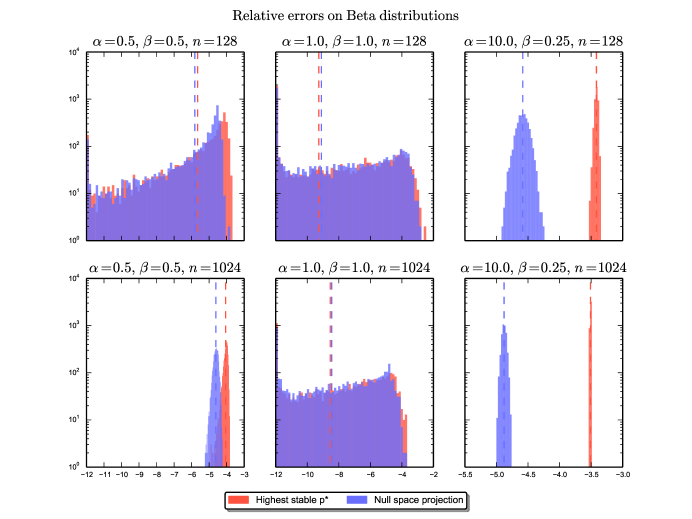
Figure 7: Relative errors on random vectors with and without null space projection. For the two approximation methods (using the highest stable $p^{*}$-norm with the heuristically chosen $p^{*}_{\max}$ or using the null space projection with $p^{*}_{\max}=64$), vectors of different lengths are sampled ($2^{12}$ repetitions) from a variety of Beta distributions. The settings for the parameters ($\alpha,\beta$) of the Beta distribution that were used, as well as the lengths of the generated vectors are shown in the titles of the subplots: $\alpha=0.5,\beta=0.5$ (bimodal with modes near zero and one); $\alpha=0.1,\beta=0.1$ (uniform distribution); $\alpha=10,\beta=0.25$ (with a strong mode near one). The red area depicts the frequencies (y-axis) of the different magnitudes of (relative) error (x-axis) when using the highest stable $p^{*}$-norm is used as an approximation of the Chebyshev norm ($p=\infty$). The blue area shows the errors with the method that performs a projection (either quadratic or linear depending on how many numerically stable $p^{*}$ are available) to estimate the Chebyshev norm.

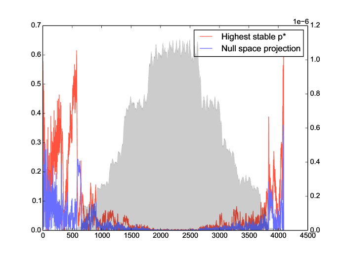
Figure 8: Relative errors on large max-convolution with and without null space projection. Max-convolution between two randomly generated vectors (both uniform vectors convolved with narrow Gaussians with uniform noise added afterward), performed with the highest stable $p^{*}$-norm (using the heuristic choice of $p^{*}_{\max}$ for problems of this size) and with null space projection (using $p^{*}_{\max}=64$). The left y-axis shows the relative error at index $m$. Associated with that, you can see the red and blue curve depicting the errors from the two different methods: Red describes the max-norm estimation using only the highest stable $p^{*}$ while purple was generated using quadratic projection at the four highest stable $p^{*}$ values (when at least four evenly spaced values are numerically stable) and linear projection at the two highest stable $p^{*}$ values (when only two $p^{*}$ are numerically stable). The results of both approaches are corrected with the affine transformation method proposed in this manuscript. In the background the gray shaded curve shows the exact result of the max-convolution at every index (to be used with the second y-axis on the right).

3.5.5 Practical runtime comparison

$k$	$2^{6}$	$2^{7}$	$2^{8}$	$2^{9}$	$2^{10}$	$2^{11}$	$2^{12}$
Naive	0.0142	0.0530	0.192	0.767	3.03	12.1	48.2
Naive (vectorized)	0.0175	0.0381	0.0908	0.251	0.790	2.75	10.1
FILL1 (Bussieck et al. (1994))	0.0866	1.09	7.21	19.4	457	—	—
Max. stable $p^{*}$, affine corrected	0.0277	0.0353	0.0533	0.0848	0.149	0.274	0.537
Projection, affine corrected	0.0236	0.0307	0.0467	0.0760	0.137	0.258	0.520

Table 3: Runtimes of different methods for max-convolution on uniform vectors of length $k$. The runtimes were gathered using the timeit package in Python. They include all preprocessing steps necessary for the algorithm (e.g. sorting prior to the FILL1 approach). The values are total runtimes (in seconds) to run $5$ repetitions on different, randomly generated vectors. FILL1 was not run on larger problems, because it ran substantially longer than the non-vectorized naive approach. On the two approximation methods presented in this manuscript, the highest stable $p^{*}$-norm approximation was run with the heuristically chosen $p^{*}_{\max}$ for problems of the appropriate size and the null space projection was run with $p^{*}_{\max}=64$.

To compare the actual runtimes of the final algorithm developed in this manuscript with a naive max-convolution and a previously proposed method from Bussieck et al. (1994), all methods were run on vectors of different random (uniform in $[0,1]$) composition and length ($k$). The first and second input vector were generated seperately but are always of same length. Table 3 shows the result of this experiment. All methods were implemented in Python, using numpy where applicable (e.g. to vectorize). A non-vectorized version of naive max-convolution was included to estimate the effects of vectorization. The approach from Bussieck et al. ran as a reimplementation based on the pseudocode in their manuscript. From their variants of proposed methods, FILL1 was chosen because of its use in their corresponding benchmark and its recommendation by the authors for having a lower runtime constant in practice compared to other methods they proposed. The method is based on sorting the input vectors and traversing the (implicitly) resulting partially ordered matrix of products in a way that not all entries need to be evaluated, while only keeping track of the so-called cover of maximal elements. FILL1 already includes some more sophisticated checks to keep the cover small and thereby reducing the overhead per iteration. Unfortunately, although we observed that the FILL1 method requires between $O(n\log(n))$ and $O(n^{2})$ iterations in practice, this per-iteration overhead results in a worst-case cost of $\log(n)$ per iteration, yielding an overall runtime in practice between $O(n\log(n)\log(n))$ and $O(n^{2}\log(n))$. As the authors state, this overhead is due to the expense of storing the cover, which can be implemented e.g. using a binary heap (recommended by the authors and used in this reimplementation). Additionally, due to the fairly sophisticated datastructures needed for this algorithm it had a higher runtime constant than the other methods presented here, and furthermore we saw no means to vectorize it to improve the efficiency. For this reason, it is not truly fair to compare the raw runtimes to the other vectorized algorithms (and it is not likely that this Python reimplementation is as efficient as the original version, which Bussieck et al. (1994) implemented in ANSI-C); however, comparing a non-vectorized implementation of the naive $O(n^{2})$ approach with its vectorized counterpart gives an estimated $\approx 5\times$ speedup from vectorization, suggesting that it is not substantially faster than the naive approach on these problems (it should be noted that whereas the methods presented here have tight runtime bounds but produce approximate results, the FILL1 algorithm is exact, but its runtime depends on the data processed). During investigation of these runtimes, we found that on the given problems, the proposed average case of $O(n\log(n))$ iterations was rarely reached. A reason might be an unrecognized violation of the assumptions of the theory behind this theoretical average runtime in how the input vectors were generated.

In contrast to the exact method from Bussieck et al. (1994), the herein proposed approximate procedure are faster whenever the input vectors are at least $128$ elements long (shorter vectors are most efficiently processed with the naive approach). The null space projection method is the fastest method presented here (because it can use a lower $p^{*}_{\max}$), although the higher density of $p^{*}$ values it uses (and thus, additional FFTs) make the runtimes nearly identical for both approximation methods.

4 Discussion

Both piecewise numerical max-convolution methods are highly accurate in practice and achieve a substantial speedup over both the naive approach and the approach proposed by Bussieck et al. (1994). This is particularly true for large problems: For the original piecewise method presented here, the $\log_{2}(\log_{1+\tau^{\frac{1}{4}}}(k))$ multiplier may never be small, but it grows so slowly with $k$ that it will be $<18$ even when $k$ is on the same order of magnitude as the number of particles in the observable universe. This means that, for all practical purposes, the method behaves asymptotically as a slightly slower $O(k\log_{2}(k))$ method, which means the speedup relative to the naive method becomes more pronounced as $k$ becomes large. For the second method presented (the null space projection), the runtime for a given relative error bound will be in $O(k\log_{2}(k))$. In practice, both methods have similar runtime on large problems.

The basic motivation of the first approach described– i.e., the idea of approximating the Chebyshev norm with the largest $p^{*}$-norm that can be computed accurately, and then convolving according to this norm using FFT– also suggests further possible avenues of research. For instance, it may be possible to compute a single FFT (rather than an FFT at each of several contours) on a more precise implementation of complex numbers. Such an implementation of complex values could store not only the real and imaginary components, but also other much smaller real and imaginary components that have been accumulated through $+$ operations, even those which have small enough magnitudes that they are dwarfed by other summands. With such an approach it would be possible to numerically approximate the max-convolution result in the same overall runtime as long as only a bounded “history” of such summands was recorded (i.e., if the top few magnitude summands—whether that be the top 7 or the top $\log_{2}(\log_{1+\tau^{\frac{1}{4}}}(k))$—was stored and operated on). In a similar vein, it would be interesting to investigate the utility of complex values that use rational numbers (rather than fixed-precision floating point values), which will be highly precise, but will increase in precision (and therefore, computational complexity of each arithmetic operation) as the dynamic range between the smallest and largest nonzero values in $L$ and $R$ increases (because taking $L^{\prime}$ to a large power $p^{*}$ may produce a very small value). Other simpler improvements could include optimizing the error vs. runtime trade-off between the log-base of the contour search: the method currently searches $\log_{2}(p^{*}_{\max})$ contours, but a smaller or larger log-base could be used in order to optimize the trade-off between error and runtime.

It is likely that the best trade-off will occur by performing the fast $p^{*}$-norm convolution with a number type that sums values over vast dynamic ranges by appending them in a short (i.e., bounded or constant size) list or tree and sums values within the same dynamic range by querying the list or tree and then summing in at the appropriate magnitude. This is reminiscent of the fast multipole algorithm (Rokhlin, 1985). This would permit the method to use a single large $p^{*}$ rather than a piecewise approach, by moving the complexity into operations on a single number rather than by performing multiple FFTs with simple floating-point numbers.

The basic motivation of the second approach described– i.e., using the sequence of $p^{*}$-norms (each computed via FFT) to estimate the maximum value– generalizes the $p^{*}$-norm fast convolution numerical approach into an interesting theoretical problem in its own right: given an oracle that delivers a small number of norms (the number of norms retrieved must be $c\in o(k)$ to significantly outperform the naive quadratic approach) about each vector $u^{(m)}$, amalgamate these norms in an efficient manner to estimate the maximum value in each $u^{(m)}$. This method may be applicable to other problems, such as databases where the maximum values of some combinatorial operation (in this case the maximum a posteriori distribution of the sum of two random variables $X+Y$) is desired but where caching all possible queries and their maxima would be time or space prohibitive. In a manner reminiscent of how we employ FFT, it may be possible to retrieve moments of the result of some combinatoric combination between distributions on the fly, and then use these moments to approximate true maximum (or, in general, other sought quantities describing the distribution of interest).

In practice, the worst-case relative error of our quadratic approximation is quite low. For example, when $p^{*}=8$ is stable, then the relative error is less than $2.3\%$, regardless of the lengths of the vectors being max-convolved. In contrast, the worst-case relative error using the original piecewise method would be $\leq k^{\frac{1}{16}}-1$, where $k$ is the length of the max-convolution result (when $n=1024$, the relative error of the original piecewise method would be $\approx 54\%$).

Of course, the use of the null space projection method is predicated on the existence of at least four sequential $p^{*}$ points, but it would be possible to use finer spacing between $p^{*}$ values (e.g., $p^{*}\in(1,1.01,1.02,1.03)$ to guarantee that this will essentially be the case as long as FFT (i.e. $p^{*}=1$) is stable. But more generally, the problem of estimating extrema from $p^{*}$-norms (or, equivalently, from the $p^{*}$-th roots of the $p^{*}$-th moments of a distribution with bounded support), will undoubtedly permit many more possible approaches that we have not yet considered. One that would be compelling is to relate the Fourier transform of the sequential moments to the maximum value in the distribution; such an approach could permit all stable $p^{*}$ at any index $m$ to be used to efficiently approximate the maximum value (by computing the FFT of the sequence of norms). Such new adaptations of the method could permit low worst-case error without any noticable runtime increase.

4.1 Multidimensional Numerical Max-Convolution

The fast numerical piecewise method for max-convolution (and the affine piecewise modification) are both applicable to matrices as well as vectors (and, most generally, to tensors of any dimension). This is because the $p^{*}$-norm (as well as the derived error bounds as an approximation of the Chebyshev norm) can likewise approximate the maximum element in the tensor $u^{(m_{1},m_{2},\ldots)}$ generated to find the max-convolution result at index $m_{1},m_{2},\ldots$ of a multidimensional problem, because the sum

$$\sum_{i_{1},i_{2},\ldots}{\left(u^{(m_{1},m_{2},\ldots)}_{i_{1},i_{2},\ldots}\right)}^{p^{*}}$$

computed by convolution corresponds to the Frobenius norm (i.e. the “entrywise norm”) of the tensor, and after taking the result of the sum to the power $\frac{1}{p^{*}}$, will converge to the maximum value in the tensor (if $p^{*}$ is large enough).

This means that the fast numerical approximation, including the affine piecewise modification, can be used without modification by invoking standard multidimensional convolution (i.e., $*$). Matrix (and, in general, tensor) convolution is likewise possible for any dimension via the row-column algorithm, which transforms the FFT of a matrix into sequential FFTs on each row and column. The accompanying Python code demonstrates the fast numerical max-convolution method on matrices, and the code can be run on tensors of any dimension (without requiring any modification).

The speedup of FFT tensor convolution (relative to naive convolution) becomes considerably higher as the dimension of the tensors increases; for this reason, the speedup of fast numerical max-convolution becomes even more pronounced as the dimension increases. For a tensor of dimension $d$ and width $k$ (i.e., where the index bounds of every dimension are $\in\{0,1,\ldots k-1\}$), the cost of naive max-convolution will be in $O(k^{2d})$, whereas the cost of numerical max-convolution is $O(k^{d}\log_{2}(k))$ (ignoring the $\log_{2}(\log_{1+\tau^{\frac{1}{4}}}(k))\leq 18$ multiplier), meaning that there is an $O(\frac{k^{d}}{d\,\log_{2}(k)})$ speedup from the numerical approach. Examples of such tensor problems include graph theory, where adjacency matrix representation can be used to describe respective distances between nodes in a network.

As a concrete example, the demonstration Python code computes the max-convolution between two $256\times 256$ matrices. The naive method required $494$ seconds, but the numerical result with the original piecewise method was computed in $3.18$ seconds (yielding a maximum absolute error of $0.0173$ and a maximum relative error of $0.0511$) and the numerical result with the null space projection method was computed in $3.99$ seconds (using $p^{*}_{\max}=512$, which corresponds to a relative error of $<0.1\%$ in the top contour, yielding a maximum absolute error of $0.0141$ and a maximum relative error of $0.0227$) and in $3.05$ seconds (using $p^{*}_{\max}=64$, which corresponds to a relative error of $<2.5\%$ in the top contour, yielding a maximum absolute error of $0.0667$ and a maximum relative error of $0.067$). Not only does the speedup of the proposed methods relative to naive max-convolution increase significantly as the dimension of the tensor is increased, no other faster-than-naive algorithms exist for max-convolution of matrices or tensors.

Multidimensional max-convolution can likewise be applied to hidden Markov models with additive transitions over multidimensional variables (e.g., allowing the latent variable to be a two-dimensional joint distribution of American and German unemployment with a two-dimensional joint transition probability).

4.2 Max-Deconvolution

The same $p^{*}$-norm approximation can also be applied to the problem of max-deconvolution (i.e., solving $M=L*_{\max}R$ for $R$ when given $M$ and $L$). This can be accomplished by computing the ratio of $FFT(M^{p^{*}})$ to $FFT(L^{p^{*}})$ (assuming $L$ has already been properly zero-padded), and then computing the inverse FFT of the result to approximate $R^{p^{*}}$; however, it should be noted that deconvolution methods are typically less stable than the corresponding convolution methods, computing a ratio is less stable than computing a product (particularly when the denominator is close to zero).

4.3 Amortized Argument for Low MSE of the Affine Piecewise Method

Although the largest absolute error of the affine piecewise method is the same as the largest absolute error of the original piecewise method, the mean squared error (MSE) of the affine piecewise method will be lower than the square of the worst-case absolute error.

To achieve the worst-case absolute error for a given contour the affine correction must be negligible; therefore, there must be two nearly vertical points on the scatter plot of $\|u^{(m_{1})}\|_{\infty}$ vs. $\|u^{(m_{1})}\|_{p^{*}}$, which are both extremes of the bounding envelope from Figure 3. Thus, there must exist two different indices $m_{1}$ and $m_{2}$ with vectors where $\|u^{(m_{1})}\|_{p^{*}}\approx\|u^{(m_{1})}\|_{\infty}$ and where

$$\|u^{(m_{2})}\|_{p^{*}}\approx\|u^{(m_{2})}\|_{\infty}k_{m_{2}}^{\frac{1}{p^{*}}}$$

(creating two vertical points on the scatter plot, and forcing that both cannot simultaneously be corrected by a single affine mapping). In order to do this, it is required to have $u^{(m_{1})}$ filled with a single nonzero value and for the remaining elements of $u^{(m_{1})}$ to equal zero. Conversely, $u^{(m_{2})}$ must be filled entirely with large, nonzero values (the largest values possible that would still use the same contour $p^{*}$). Together, these two arguments place strong constraints on the vectors $L^{\prime}$ and $R^{\prime}$ (and transitively, also constrains the unscaled vectors $L$ and $R$): On one hand, filling $u^{(m_{1})}$ with $k_{m_{1}}-1$ zeros requires that $k_{m_{1}}-1$ elements from either $L$ or $R$ must be zero (because at least one factor must be zero to achieve a product of zero). On the other hand, filling $u^{(m_{2})}$ with all large-value nonzeros requires that $k_{m_{2}}$ elements of both $L$ and $R$ are nonzero. Together, these requirements stipulate that both $k_{m_{1}}-1+k_{m_{2}}\leq k$, because entries of $L$ and $R$ cannot simultaneously be zero and nonzero. Therefore, in order to have many such vertical points, constrains the lengths of the $u^{(m_{1})},u^{(m_{2})},u^{(m_{3})},\ldots$ vectors corresponding to those points. While the worst-case absolute error bound presumes that an individual vector $u^{(m)}$ may have length $k$, this will not be possible for many vectors corresponding to vertical points on the scatter plot. For this reason, the MSE will be significantly lower than the square of the worst-case absolute error, because making a high affine-corrected absolute error on one index necessitates that the absolute errors at another index cannot be the worst-case absolute error (if the sizes of $L$ and $R$ are fixed).

5 Availability

Code for exact max-convolution and the fast numerical method (which includes both $\|\cdot\|_{p^{*}}$ and null space projection methods) is implemented in Python and available at https://bitbucket.org/orserang/fast-numerical-max-convolution. All included code works for numpy arrays of any dimension, i.e. tensors).

6 Acknowledgments

We would like to thank Mattias Frånberg, Knut Reinert, and Oliver Kohlbacher for the interesting discussions and suggestions. J.P. acknowledges funding from BMBF (Center for Integrative Bioinformatics, grant no. 031A367). O.S. acknowledges generous start-up funds from Freie Universität Berlin and the Leibniz-Institute for Freshwater Ecology and Inland Fisheries.

References

• Boyer et al. (2013) Marc Boyer, Guillaume Dufour, and Luca Santinelli. Continuity for network calculus. In 21st International Conference on Real-Time Networks and Systems, page 235, New York, New York, USA, October 2013. ACM Press.
• Bremner et al. (2006) David Bremner, Timothy M Chan, Erik D Demaine, Jeff Erickson, Ferran Hurtado, John Iacono, Stefan Langerman, and Perouz Taslakian. Necklaces, convolutions, and x+ y. In Algorithms–ESA 2006, pages 160–171. Springer, 2006.
• Bussieck et al. (1994) Michael Bussieck, Hannes Hassler, Gerhard J. Woeginger, and Uwe T. Zimmermann. Fast algorithms for the maximum convolution problem. Operations Research Letters, 15(3):133–141, April 1994.
• Eddington (1923) Arthur Stanley Eddington. Mathematical Theory of Relativity. Cambridge University Press, London, 1923.
• Horn and Johnson (1999) Roger A Horn and Charles R Johnson. Matrix analysis. Cambridge university press, 1999.
• Ritter and Wilson (2000) Gerhard X. Ritter and Joseph N. Wilson. Handbook of Computer Vision Algorithms in Image Algebra. CRC Press, Inc., August 2000.
• Rokhlin (1985) Vladimir Rokhlin. Rapid solution of integral equations of classical potential theory. Journal of Computational Physics, 60(2):187–207, 1985.
• Serang (2014) Oliver Serang. The probabilistic convolution tree: efficient exact Bayesian inference for faster LC-MS/MS protein inference. PLOS ONE, 9(3):e91507, January 2014.
• Serang (2015) Oliver Serang. A fast numerical method for max-convolution and the application to efficient max-product inference in bayesian networks. Journal of Computational Biology, 22:770–783, 2015.
• Serang et al. (2010) Oliver Serang, Michael J MacCoss, and William Stafford Noble. Efficient marginalization to compute protein posterior probabilities from shotgun mass spectrometry data. Journal of Proteome Research, 9(10):5346–57, October 2010.
• Sun and Yang (2002) Ning Sun and Zaifu Yang. The max-convolution approach to equilibrium analysis. Technical report, Bielefeld University, Center for Mathematical Economics, December 2002.
• Zach et al. (2008) Christopher Zach, David Gallup, and Jan-Michael Frahm. Fast gain-adaptive KLT tracking on the GPU. In 2008 IEEE Computer Society Conference on Computer Vision and Pattern Recognition Workshops, pages 1–7. IEEE, June 2008.