The VLT-FLAMES Tarantula Survey

We investigate the multiplicity properties of 408 B-type stars observed in the 30 Doradus region of the Large Magellanic Cloud with multi-epoch spectroscopy from the VLT-FLAMES Tarantula Survey (VFTS). We use a cross-correlation method to estimate relative radial velocities from the helium and metal absorption lines for each of our targets. Objects with significant radial-velocity variations (and with an amplitude larger than 16 km s^-1) are classified as spectroscopic binaries. We find an observed spectroscopic binary fraction (defined by periods of $<$10^3.5 d and mass ratios $>$ 0.1) for the B-type stars, $f_{\rm B}$(obs) $=$ 0.25 $\pm$ 0.02, which appears constant across the field of view, except for the two older clusters (Hodge 301 and SL 639). These two clusters have significantly lower binary fractions of 0.08 $\pm$ 0.08 and 0.10 $\pm$ 0.09, respectively. Using synthetic populations and a model of our observed epochs and their potential biases, we constrain the intrinsic multiplicity properties of the dwarf and giant (i.e. relatively unevolved) B-type stars in 30 Dor. We obtain a present-day binary fraction $f_{\rm B}$(true) $=$ 0.58 $\pm$ 0.11, with a flat period distribution. Within the uncertainties, the multiplicity properties of the B-type stars agree with those for the O stars in 30 Dor from the VFTS.

1 Introduction

The presence of a close companion can significantly influence the evolution of massive stars (e.g. Podsiadlowski et al. 1992; Langer et al. 2008; Eldridge et al. 2011), but the prevalence of mass transfer in such systems has only recently been realised. A consequence of the high spectroscopic binary fractions inferred for massive stars in the Galaxy (e.g. Mason et al. 2009; Sana et al. 2008, 2009, 2011; Kiminki & Kobulnicky 2012; Chini et al. 2012; Sota et al. 2014) is that the majority of massive stars may be born as part of, and reside within, multiple systems (Kobulnicky & Fryer 2007; Sana et al. 2012). Additionally, stars that currently appear to be single may have evolved from binary systems (de Mink et al. 2014), with important consequences on their inferred evolutionary histories (de Mink et al. 2011, 2013).

The multiplicity fraction of B-type stars has been investigated in some Galactic clusters (e.g. Raboud 1996) but, to date, most studies of the multiplicity of high-mass stars have focused on the more massive O-type objects (e.g. Sana & Evans 2011, and references therein). Substantial spectroscopic samples of B-type stars in the Galaxy and Magellanic Clouds are available from large spectroscopic programmes (e.g. Evans et al. 2005, 2006; Martayan et al. 2006, 2007), but they have lacked sufficient time sampling to investigate the role of binarity in the observed populations.

One of the primary motivations for the VLT-FLAMES Tarantula Survey (VFTS, Evans et al. 2011, hereafter Paper I) is to investigate the multiplicity properties of the massive stars in the 30 Doradus region of the Large Magellanic Cloud (LMC). To this end, the VFTS obtained multi-epoch spectroscopy of $\sim$800 O- and early B-type stars. The observed spectroscopic binary fraction, $f_{\rm O}$(obs), of the 360 O-type stars in the VFTS was found to be $f_{\rm O}$(obs) $=$ 35 $\pm$ 3% (Sana et al. 2013, hereafter Paper VIII); once the observational biases were taken into account, this gave an intrinsic binary fraction, $f_{\rm O}$(true) $=$ 51 $\pm$ 4%.

Here we investigate the multiplicity properties of the B-type stars observed by the VFTS. One of our objectives is an estimate of their present-day observed spectroscopic binary fraction, $f_{\rm B}$(obs), where $f$ defines the fraction of targets where Doppler shifts are detected (rather than the total fraction of all stars), probing separations with orbital periods of up to approximately 10 years (e.g. see Fig. 1 from Sana & Evans 2011). For consistency with the analysis by Sana et al. (2012) and in Paper VIII, we adopt the same definition of a spectroscopic binary as a system with a period of $<$10^3.5 d and a mass ratio of $>$ 0.1. The present-day binary fraction can then be used to constrain the minimum binary fraction of B-type stars at their birth (with initial masses of $\gtrsim$ 8  $\mathrm{M}_{\odot}$). Ultimately, in combination with the results for the O-type stars (from Paper VIII), our aim is to determine the fraction of massive stars that might be affected by binary interaction during their lives, which will influence their evolution and the properties of their final explosions. Indeed, assuming the form of the stellar mass-function from Kroupa (2001), around two thirds of the progenitors of core-collapse supernovae were probably early B-type stars when on the main sequence.

After a brief summary of the observations in Section 2, we describe the methods used to identify spectroscopic binaries in Section 3. We present our results in Section 4 and investigate the intrinsic properties of the binary population in Section 5. Concluding remarks are given in Section 6.

2 Observations

The VFTS spectra were obtained with the Fibre Large Array Multi-Element Spectrograph (FLAMES, Pasquini et al. 2002) on the Very Large Telescope (VLT). Classifications for the 438 B-type stars observed in the VFTS were given by Evans et al. (2015). These are located in the main clusters in the 30 Dor region (i.e. NGC 2070, NGC 2060, Hodge 301, SL 639) and the local field population (see Fig. 4 from Evans et al.). All of the spectra were obtained using the fibre-fed Medusa–Giraffe mode of FLAMES, so the sample does not include stars in R136, the young massive cluster at the core of 30 Dor, which is too densely populated for effective use of the Medusa fibres.

This paper presents a radial-velocity (RV) analysis of the multiple observations of the B-type stars with the LR02 setting of the Giraffe spectrograph. The observations spanned 10–12 months for most targets, with an extended baseline of 22 months for 31 targets, due to a reobservation for operational reasons. Two or three consecutive exposures were obtained on any given night, with the longer-term sampling designed to optimise detection of binaries with periods up to $\sim$200 d, given scheduling constraints. (The detection probability decreases significantly for longer-period systems; see e.g. Fig. 8 of Paper VIII, ). Further details regarding target selection, data reduction, and the observation dates are given in Paper I.

Absolute RVs for the B-type sample were provided by Evans et al. (2015), which are either the mean of estimates from each observation or, where binary motion was suspected, the estimate from a particular observation. For 30 stars the spectra were not of sufficient quality to allow reliable estimates of the absolute RVs, and these stars have been excluded from our sample. As these span a range of spectral types and morphologies (including examples of Be-type stars), they should not unduly influence the results. A further five targets are the double-lined binaries identified by Evans et al. (2015), namely: VFTS 112, 199, 240, 637, and 698. It was challenging to obtain multi-epoch RV estimates to the same standard as those used for the analysis in Section 3, but their binary natures were easily revealed by variations in their spectra (indicative of binary motion, rather than simply composite spectra).

Therefore, in total we investigated the multiplicity of 408 stars, comprised of 361 dwarfs and giants (i.e. relatively unevolved objects) and 47 supergiants (defined as having a logarithmic gravity, $\log$ g $\leq$ 3.3 dex, see McEvoy et al. 2015); hereafter these are referred to as the ‘unevolved’ and ‘supergiant’ samples.

3 Radial velocities

3.1 Methodology

We began by examining the 403 single-lined targets for evidence of RV variability. An important aspect of RV studies in early-type stars concerns the choice of diagnostic lines. Our preferred features for B-type stars would be their intrinsically narrow metal absorption lines. However, the large variation in the intensity of these lines with spectral type means they would not provide a homogeneous set of estimates on their own. We therefore employed both helium and metal absorption lines (see Table 1) to obtain a range of independent RV estimates, as permitted by the signal-to-noise (S/N) ratio of the data and the spectral type of each target.

For each of the lines available from Table 1, relative RV estimates ($v_{i}$) were obtained for each LR02 spectrum ($i$) of a given target from cross-correlation of the data with an adopted reference spectrum (typically that for the object with the largest number of counts in the continuum around 4200 Å). This approach has been widely used (see e.g. Marocco et al. 2015; Manick et al. 2015; Robertson & Mahadevan 2014, and references therein), with our methodology being similar to that used by Marocco et al. (2015).

The spectral region used in the cross-correlation analysis depends on the width of the spectral feature being considered. In turn this depends on both its intrinsic width (e.g. diffuse helium lines will be far broader than non-diffuse helium lines or metal lines) and on the stellar projected rotational velocity. The projected rotational velocity estimates from Dufton et al. (2013) for the subset of our sample which have no significant radial-velocity shifts cover a wide range. The distribution is bi-modal with peaks at $v_{\mathrm{e}}\sin i$$\simeq$ 20 and 180 km s^-1 , coupled with a long tail to around 400 km s^-1 . The latter would equate to a full-width-half maximum rotational broadening of about 6Å (depending on the stellar wavelength). Given this wide variation in the width of spectral features, the choice of spectral regions for each line was made subjectively. The principle criteria were to minimise the region selected (to maximise the cross-correlation signal), whilst ensuring both complete coverage of the feature and sufficient continuum to fully characterise the cross-correlation function.

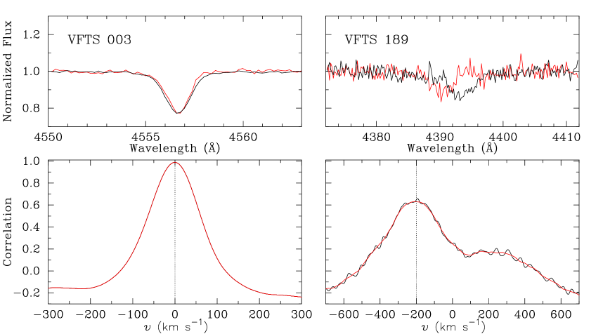
Figure 1: Examples of the methodology to estimate radial-velocity shifts between the spectra. Left-hand panels: VFTS 003 is a relatively bright narrow-lined supergiant. The upper panel shows the Si iii 4553Å line in the template spectrum (MJD $=$ 54804.148, black line) and at MJD $=$ 55108.309 (red). The lower panel shows the original (black line) and smoothed (red) cross-correlation function in velocity space; no significant velocity shifts were found for this target. Right-hand panels: VFTS 189 is a relatively faint, broad-lined, main-sequence star. The upper panel shows the He i 4388Å line in the template spectrum (MJD $=$ 54867.160, black) and at MJD $=$ 54824.242 (red). The lower panel shows the original and smoothed cross-correlation functions in velocity space; the estimated radial-velocity shift between these was $\sim$200 km s^-1 .

The position of the maximum could be affected by spurious structure in the cross-correlation function, so our method was informed by the projected equatorial rotation velocities ($v_{\mathrm{e}}\sin i$) for each star from Dufton et al. (2013). For supergiants and narrow-lined spectra ($v_{\mathrm{e}}\sin i$ $\leq$ 150 km s^-1 ) the cross-correlation function was smoothed by a 5-point moving average (equivalent to $\sim$50 km s^-1 in velocity space). For stars rotating more rapidly, a 55-point moving average was used, to militate against the increased influence of random noise in the cross-correlation function; this method was tested for the narrow-lined spectra giving, in general, identical results.

The procedure is illustrated for two cases in Fig. 1, viz. the Si iii 4553Å line in the narrow-lined bright supergiant VFTS 003 (B1 Ia⁺) and the He i 4388Å diffuse line in the relatively rapidly rotating ($v_{\mathrm{e}}\sin i$$\simeq$ 212 km s^-1 ) and fainter main-sequence star, VFTS 189 (B0.7: V); as such they illustrate the range in quality of the available observational data.

The relatively narrow absorption lines and high S/N of the supergiant spectra meant that all of the metal and helium lines listed in Table 1 could be used for the RV analysis; this was also possible for $\sim$20% of the (non-supergiant) narrow-lined objects. For more-rapidly-rotating stars ($v_{\mathrm{e}}\sin i$ $\geq$ 150 km s^-1 ), only the helium lines were generally available.

Table 1: Absorption lines used to estimate relative radial velocities for the B-type spectra.

Ion	$\lambda$ (Å)	Type
O ii	4080	Group
He i	4009	Singlet
He i	4026	Triplet
He i	4121	Triplet
He i	4144	Singlet
He i	4169	Singlet
O ii	4317	Doublet
He i	4388	Singlet
O ii	4414	Doublet
He i	4438	Singlet
He i	4471	Triplet
Si iii	4553	Singlet

The relative RVs for each observation of 370 of our targets are presented in Table 2; the remaining 33 targets were affected by nebular contamination and are discussed in the next section, while a RV analysis was not attempted for the five targets classified as SB2 systems. We note that non-zero estimates arise from cross-correlation of the template spectra with themselves, with a systematic median offset of $-$0.28 km s^-1  arising from the fits to the cross-correlation function. In the context of our analysis of relative velocities and the adopted criteria to identify binaries (Section 3.3) such measurement uncertainties are not significant.

Table 2: Relative radial-velocity (RV) estimates for the available lines in each observation (cf. the adopted template spectrum for each star). Values for the first three VFTS targets are shown; the full table is available online.

VFTS	MJD	Relative radial velocities [km s-1 ]
		Si iii	O ii	O ii	O ii	He i	He i	He i	He i	He i	He i	He i	He i
		$\lambda$4553	$\lambda$4080	$\lambda$4317	$\lambda$4414	$\lambda$4026	$\lambda$4471	$\lambda$4009	$\lambda$4144	$\lambda$4388	$\lambda$4121	$\lambda$4438	$\lambda$4169
001	54815.254	…	…	…	…	$-$25.48	…	…	…	10.55	…	…	…
001	54815.277	…	…	…	…	$-$6.33	…	…	…	$-$31.42	…	…	…
001	54815.305	…	…	…	…	$-$13.05	…	…	…	$-$1.63	…	…	…
001	54815.328	…	…	…	…	$-$22.53	…	…	…	$-$28.72	…	…	…
001	54859.211	…	…	…	…	$-$9.27	…	…	…	$-$9.76	…	…	…
001	54859.230	…	…	…	…	6.93	…	…	…	$-$19.24	…	…	…
001	54891.062	…	…	…	…	$-$32.84	…	…	…	$-$13.82	…	…	…
001∗ (S)	54891.082	…	…	…	…	$-$0.44	…	…	…	$-$0.28	…	…	…
003	54804.082	0.76	2.83	$-$0.57	0.92	$-$0.44	1.05	$-$0.05	$-$1.98	2.43	$-$0.56	$-$1.86	…
003	54804.105	0.76	1.33	0.79	0.92	$-$1.91	1.05	1.44	$-$0.55	1.08	0.88	0.81	…
003	54804.125	0.76	2.83	0.79	0.92	1.04	1.05	1.44	$-$0.55	1.08	0.88	0.81	…
003∗ (V)	54804.148	$-$0.54	$-$0.17	$-$0.57	$-$0.42	$-$0.44	$-$0.28	$-$0.05	$-$0.55	$-$0.28	$-$0.56	$-$0.53	…
003	54804.168	0.76	1.33	0.79	$-$0.42	$-$0.44	1.05	$-$0.05	$-$1.98	$-$0.28	$-$0.56	$-$0.53	…
003	54804.191	0.76	$-$0.17	0.79	$-$0.42	1.04	1.05	1.44	$-$0.55	$-$0.28	$-$0.56	$-$0.53	…
003	54836.219	4.65	2.83	2.16	0.92	8.40	10.35	2.92	2.30	3.78	2.31	6.14	…
003	54836.238	4.65	2.83	2.16	0.92	8.40	10.35	4.41	2.30	5.14	2.31	0.81	…
003	54836.266	3.35	2.83	2.16	0.92	8.40	10.35	4.41	2.30	5.14	2.31	0.81	…
003	54836.285	4.65	2.83	2.16	0.92	6.93	11.67	2.92	2.30	3.78	2.31	3.47	…
003	54867.086	13.73	8.84	11.72	7.64	17.24	19.64	13.33	12.28	14.62	10.92	14.14	…
003	54867.109	15.02	10.34	13.09	6.29	17.24	20.97	13.33	12.28	13.26	8.05	7.47	…
003	55108.309	$-$0.54	$-$0.17	$-$0.57	$-$0.42	$-$0.44	$-$1.61	1.44	$-$1.98	$-$2.99	0.88	$-$3.19	…
005	54815.254	…	…	…	…	$-$7.80	…	…	6.58	$-$1.63	…	…	…
005	54815.277	…	…	…	…	$-$0.44	…	…	$-$0.55	2.43	…	…	…
005	54815.305	…	…	…	…	18.71	…	…	$-$17.67	3.78	…	…	…
005	54815.328	…	…	…	…	$-$7.80	…	…	16.56	$-$1.63	…	…	…
005	54859.211	…	…	…	…	$-$1.91	…	…	17.99	24.10	…	…	…
005	54859.230	…	…	…	…	$-$10.75	…	…	8.00	13.26	…	…	…
005	54891.062	…	…	…	…	$-$12.22	…	…	$-$6.26	$-$1.63	…	…	…
005∗ (S)	54891.082	…	…	…	…	$-$0.44	…	…	$-$0.55	$-$0.28	…	…	…
005	55113.309	…	…	…	…	$-$13.69	…	…	0.87	21.39	…	…	…
005	55113.328	…	…	…	…	$-$0.44	…	…	10.86	11.91	…	…	…

3.2 Nebular contamination

There is considerable nebulosity across the 30 Dor region, which contaminates the FLAMES spectroscopy to varying degrees. This can complicate the RV estimates by the introduction of additional structure (centred at $\Delta$RV $\simeq$ 0 km s^-1 ) in the cross-correlation profiles of the helium lines. For the majority of our targets the nebular emission was sufficiently weak that any associated structure in the cross-correlation function was minor, and robust RV estimates were possible. However, the contamination was more significant for 33 of our targets, so we employed a modified method where all exposures for a given date were merged to improve the S/N, and then analysed as for the other spectra. The relative velocities from this approach for these targets are given in Table 3.

3.3 Criteria for binarity

Our strategy for binary detection relies on statistical criteria, with the significance threshold adopted such that it limited the number of false positives. Thus, while some binaries may remain undetected, this systematic approach enables modelling of the observational biases. For consistency, we adopted similar criteria for binarity to those used in the analysis of the O-type stars (Paper VIII), such that an object is considered a spectroscopic binary if at least one pair of RV estimates satisfies simultaneously

$$\frac{|v_{i}-v_{j}|}{\sqrt{\sigma_{i}^{2}+\sigma_{j}^{2}}}>4.0\leavevmode\nobreak\ \leavevmode\nobreak\ \leavevmode\nobreak\ {\rm and}\leavevmode\nobreak\ \leavevmode\nobreak\ \leavevmode\nobreak\ |v_{i}-v_{j}|>\Delta{\rm RV}_{\rm min},$$ (1)

where $v_{i}$ is the mean relative RV for exposure $i$ with respect to the template, and $\sigma_{i}$ is its associated standard deviation. The choice of 4.0 for the confidence threshold for a detection was guided by the number of false positives one may statistically expect given the sample size, the uncertainties of the RV estimates, and the number of RV pairs. Using Monte Carlo simulations, adopting 4.0 leads to fewer than 0.2 false detections for the whole sample, which is sufficient for our purposes. Furthermore, this threshold value is identical to that adopted in Paper VIII, ensuring a consistent approach.

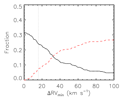
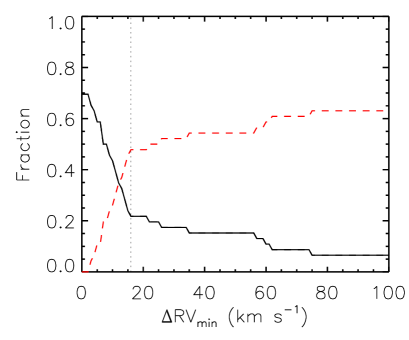
Figure 2: Upper panel: Inferred binary fraction as a function of the adopted threshold velocity ($\Delta$RV_min) for the unevolved (dwarf/giant) B-type stars in our sample (solid line). The dashed line shows the corresponding fraction that would have been classified as binary candidates but failed the $\Delta$RV_min criterion. Lower panel: As for the upper panel, but for the supergiants. In both plots the vertical dotted line indicates the adopted threshold of 16 km s^-1 .

The choice of $\Delta$RV_min was particularly important for the supergiants, for which precise RVs could be determined given their high S/N and relatively narrow-lined profiles. Small ranges of variations ($\simeq$ 5-10 km s^-1 ) could indicate a binary companion, but may also result from atmospheric activity or pulsations (e.g. Taylor et al. 2014).

The percentage of binary candidates identified for different values of $\Delta$RV_min is illustrated in Fig. 2. For the unevolved stars, no clear break is seen. However, the fraction of RV-variable objects for the supergiants presents a clear kink around $\Delta$RV_min $=$ 16 km s^-1   with samples plausibly dominated by binarity and intrinsic variability above and below the kink, respectively. This is a slightly lower threshold than that adopted in Paper VIII for the O-type stars (i.e. $\Delta$RV_min $=$ 20 km s^-1 ), but is consistent with the lower masses of early B-type stars (cf. those for O stars).

Objects fulfilling both criteria of Eq. 1 (with $\Delta$RV_min $=$ 16 km s^-1 ) are considered as spectroscopic binaries. Those fulfilling the first condition of Eq. 1, but with a maximum $\Delta$RV in the range of 5 to 16 km s^-1  are identified as ‘RV variables’, with the variations attributable to either binarity or intrinsic variability. The remaining objects are presumed to be single stars for the purposes of the following discussion.

Table 3: Relative radial-velocities (RV) for spectra with significant nebular contamination but which estimates were possible from combining the spectra from each night (see Section 3.2). Values for the first three entries are shown; the full table is available online.

VFTS	MJD	Relative radial velocities [km s-1 ]
		He i	He i	He i	He i
		$\lambda$4388	$\lambda$4144	$\lambda$4026	$\lambda$4471
004∗ (S)	54767	0.39	0.44	0.29	$-$1.42
004	54827	$-$14.28	$-$15.10	$-$12.47	$-$71.61
004	54828	$-$39.97	$-$59.7	$-$23.65	$-$14.02
004	54860	$-$10.62	$-$3.45	17.85	0.37
004	54886	$-$60.14	$-$40.36	$-$12.47	$-$23.02
004	55114	53.58	$-$3.45	$-$58.75	$-$28.42
010	54767	26.80	5.19	$-$14.43	6.94
010	54827	9.20	$-$12.24	$-$26.21	$-$32.39
010∗ (S)	54860	$-$0.28	0.44	$-$1.17	$-$0.34
010	54886	$-$39.55	40.07	$-$8.54	…
010	55114	4.88	41.65	$-$17.38	…
054∗ (S)	54767	$-$0.28	$-$0.27	6.93	$-$0.28
054	54827	20.03	$-$28.95	$-$15.16	$-$18.88
054	54860	49.82	24.11	8.40	19.64
054	54886	$-$21.94	$-$23.22	$-$60.82	$-$37.47
054	55114	$-$21.94	31.28	$-$65.24	$-$33.49

4 The binary sample

4.1 Observed binary fraction

Employing the criteria in Eq. 1 to analyse the RV estimates in Tables 2 and 3, combined with the SB2 systems, we found 90 binaries in the unevolved sample and 11 binaries in the supergiants. The observed binary fractions are therefore $25\pm 2$% and $23\pm 6$%, respectively, where binomial statistics have been used to compute the error bars (see Sana et al. 2009). An additional 23 unevolved stars and 17 supergiants were detected as RV variables, comprising $6\pm 1$% and $36\pm 7$% of their respective samples. The lower limit for the spectroscopic binary fraction for the entire VFTS B-type sample (including the supergiants and SB2 systems) is $f_{\rm B}$(obs) $=$ 25 $\pm$ 2%, with RV variables accounting for a further $10\pm 1$% of the stars.

4.2 Supergiants

The effects of macroturbulence in blue supergiants appear to be linked to line-profile variations (Simón-Díaz et al. 2010), so adoption of $\Delta$RV_min $=$ 16 km s^-1  in Section 3.3 was particularly important for these objects in the VFTS sample (for which the uncertainties on the RV estimates are relatively small). To investigate the nature of RV variations in the supergiants further we employed the same procedures as those used by Simón-Díaz et al. (2010) to quantify the potential role of macroturbulence in our targets.

In general, this additional analysis confirmed the classifications regarding multiplicity using the criteria from Section 3.3. However, there are four objects (VFTS 420, 423, 541, and 829) classified as RV variables (with 12 $<$ $\Delta$RV $<$ 15 km s^-1 ) for which the results are consistent with minimal macroturbulence, thereby strengthening the case for orbital RV variations. Conversely, VFTS 591, classified as a binary using the above criteria, has a relatively large contribution from macroturbulence and thus might be a single star. Revising these classifications would increase the binary fraction for the supergiants from 23 $\pm$ 6% to 30 $\pm$ 7%, i.e. within the statistical uncertainties, indicating that uncertainties due to macroturbulence do not appear to strongly influence the result.

4.3 Timescales for detected variations

The upper panel of Figure 3 shows the cumulative distribution of the maximum RV variation for our objects with estimates in Tables 2 and 3 which are classified as binaries. Approximately $\sim$20% of the objects in the binary sample have $\Delta$RV $>$ 100 km s^-1 ; these are probably short-period binaries.

The lower panel of Figure 3 shows the minimum time difference for which significant RV-variations are detected. The minimum elapsed time between the LR02 observations of eight of the nine fibre configurations was typically between one and seven days (except for Field C, with a minimum separation of 28 days, see Appendix of Paper I); hence we expect that the RV detectability is principally determined by the properties of the stars rather than the cadence of the observations. Variations are seen over timescales of one to ten days for $\sim$30% of the sample (although this should not be taken as a direct measure of their orbital periods), while a relatively small number of the detected systems ($\simeq$15%) only show variations over several hundreds of days. Full characterisation of the individual orbital properties of the detected binaries will require comprehensive multi-epoch spectroscopy.

4.4 Spatial variations

We searched for variations in the observed binary fraction in the different structures in the region, i.e. NGC 2070, NGC 2060, Hodge 301, SL 639 (adopting the same definitions as those used by Evans et al. 2015), and the field population. The binary fractions and numbers of targets in each subsample are summarised in Table 4. The observed fractions are marginally larger in NGC 2070 and NGC 2060, but remain within the estimated uncertainties for those in the field population. For the two older clusters, the observed fractions for the unevolved targets appear to be slightly lower.

Figure 3: Cumulative fractions of the maximum RV amplitude detected (upper panel) and the minimum time difference corresponding to significant RV-variations (lower panel) for the detected binaries in the B-type sample.

Table 4: Observed binary fraction for various subpopulations in the 30 Dor region.

Region	Non-supergiants		Supergiants		All
	$N_{\mathrm{obj}}$	$f_{\rm B}$(obs)	$N_{\mathrm{obj}}$	$f_{\rm B}$(obs)	$N_{\mathrm{obj}}$	$f_{\rm B}$(obs)
NGC 2070	93	0.27 $\pm$ 0.05	16	0.31 $\pm$ 0.12	109	0.28 $\pm$ 0.04
NGC 2060	29	0.34 $\pm$ 0.05	3	0.00 $\pm$ 0.11	32	0.31 $\pm$ 0.08
Hodge 301	12	0.08 $\pm$ 0.08	3	0.00 $\pm$ 0.27	15	0.07 $\pm$ 0.06
SL 639	10	0.10 $\pm$ 0.09	4	0.25 $\pm$ 0.27	14	0.14 $\pm$ 0.09
Field	217	0.24 $\pm$ 0.03	21	0.24 $\pm$ 0.22	238	0.25 $\pm$ 0.03
All	361	0.25 $\pm$ 0.02	47	0.23 $\pm$ 0.06	408	0.25 $\pm$  0.02

4.5 Brightness variations

We also investigated the binary fraction as a function of the brightness of our targets, employing $K_{\rm s}$-band magnitudes from the VISTA Magellanic Clouds Survey (Cioni et al. 2011). As shown in Fig. 4, there are no obvious trends, suggesting that the binary fraction is mostly uniform over more than two orders of magnitude in brightness.

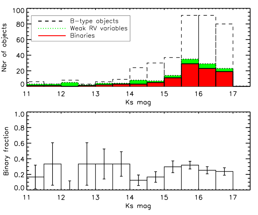
Figure 4: Observed binary fraction as a function of $K_{\rm s}$ magnitude.

5 Intrinsic multiplicity properties

The observed binary fraction of the 408 B-type stars is $f_{\rm B}$(obs) $=$ 0.25 (i.e. 96 positive detections through RV variations and 5 SB2 system). Because of the cadence of the FLAMES observations, the S/N of our data, and the orientation of the binary systems with respect to our line of sight, some binaries will have eluded detection. Thus, ignoring statistical uncertainties, $f_{\rm B}$(obs) represents a lower limit on the true binary fraction of B-type stars in 30 Dor.

To estimate the intrinsic binary fraction we modelled our criteria for binarity and estimated our observational biases and detection sensitivities. In this analysis we ignored the five SB2 systems discussed in Section 2 as their double-lined nature prevented us from obtaining reliable estimates of the RV variation of the primary stars. Therefore, as a result of this approximation, the intrinsic binary fraction that we recover may be lower than the true value by a few percentage points. However, this remains well within the uncertainty of the method (see below).

As discussed in Paper VIII, the detection probability of a given binary system depends on the properties of the data (uncertainty of RV estimates, time sampling) and on the properties of the RV signal that one is trying to detect. The latter is directly determined by the orbital properties of the system. The (in)completeness of the VFTS campaign therefore depends on the distribution of the orbital parameters of the parent binary population (predominantly the orbital periods, mass ratios, and eccentricities). Unfortunately, these quantities are unknown. Thus, to constrain the intrinsic multiplicity properties of the binaries in our sample, we follow the approach implemented in Paper VIII for the analysis of the O-type stars.

Using a Monte Carlo method, we synthesised populations of stars with specified parent orbital distributions. Taking into account the measurement uncertainties and the time sampling of each object, we sought to reproduce the observational quantities in three aspects: (i) the observed binary fraction $f_{\rm B}$(obs), (ii) the cumulative distribution of the maximum amplitude, CDF($\Delta$RV), of significant RV variations (see Fig. 3, upper panel) and (iii) the cumulative distribution of the minimum time separation, CDF($\Delta$HJD), between any pair of RV points that differ significantly from one another (see Fig. 3, lower panel).

The quality of the match between observations and simulations was assessed using a global merit function ($\Xi^{\prime}$). This was defined as the product of the Kolmogorov-Smirnov (KS) probabilities between the synthetic CDFs for $\Delta$RV and $\Delta$HJD and their observed distributions, and of the Binomial probability that describes the chance to obtain the same number of detected binaries ($N_{\rm bin}$) as in our sample, given the simulated observed binary fraction $f_{\rm B}({\rm obs})^{\rm simul}$ and the sample size $N$:

$$\Xi^{\prime}=P_{\rm KS}(\Delta{\rm RV})\times P_{\rm KS}(\Delta{\rm HJD})\times B(N_{\rm bin},N,f_{\rm B(obs)}^{\rm simul}).$$ (2)

The method is described further in Paper VIII. Stellar masses in the simulated populations were randomly drawn from a mass-function over a given stellar range. We can reasonably assume that the unevolved stars follow a standard mass-function (e.g. Kroupa 2001), but the situation may be different for the supergiants, many of which would have been born as higher-mass stars, which could have experienced considerable evolution prior to their current phase (e.g. mass lost via stellar winds, binary interactions). Therefore, we focus on the 357 unevolved B-type stars in our sample (which does not include the four SB2 systems with unevolved stars; cf. the numbers in Table 4).

As in Paper VIII, we considered orbital periods ($P$), mass-ratios ($q=M_{2}/M_{1}$) and eccentricities ($e$) over ranges of 0.15 $\leq$ $\log(P/{\rm d})$ $\leq$ 3.5, 0.1 $\leq$ q $\leq$ 1.0 and 0 $<$ e $\leq$ 0.9, respectively. We adopted power-laws to describe the distributions of the orbital parameters: $f_{\rm P}$ $\propto$ $(\log P/{\rm d})^{\pi}$, $f_{\rm q}$ $\propto$ $q^{\kappa}$ and $f_{\rm e}$ $\propto$ $e^{\eta}$. We varied $\pi$, $\kappa$ and the intrinsic number of binaries to best reproduce the observed quantities CDF($\Delta$RV), CDF($\Delta$HJD) and $f_{\rm B}$(obs). Our method was insensitive to the eccentricity distribution and we could not constrain $\eta$. As in our analysis of the O-stars, we adopted the value obtained from O-type binaries in Galactic open clusters, $\eta$ $=$ $-$0.5 (Sana et al. 2012). While there is no guarantee that this value is appropriate, it preserves the homogeneity of the analysis of the O- and B-type populations from the VFTS. The range of values explored for $f_{\rm B(true)}$, $\pi$ and $\kappa$ are given in Table 5, and the criteria to identify binarity in the Monte Carlo simulations are those described in Section 3.3.

Table 5: Properties of the Monte Carlo grid. The first three rows provide information on the orbital distributions: physical parameter (Col. 1), probability-density function (Col. 2) and applicability domain (Col. 3). Cols. 4 to 6 give the quantity, investigated range and step size in the grid.

Parameter	pdf	Domain	Var.	Range	Step
$P$ (d)	$(\log_{10}P)^{\pi}$	0.15 - 3.5	$\pi$	$-$2.50 - $+$2.50	0.1
$q$	$q^{\kappa}$	0.1 - 1.0	$\kappa$	$-$3.50 - $+$1.50	0.1
$e$	$e^{\eta}$	$10^{-5}$ - 0.9	$\eta$	$-$0.5 (fixed)	$n/a$
$f_{\rm B(true)}$	$n/a$	$n/a$	$f_{\rm B(true)}$	$+$0.40 - $+$1.00	0.02

Fig. 6 shows the behaviour of $\Xi^{\prime}$ when varying $f_{\rm B(true)}$, $\pi$ and $\kappa$ and Fig. 6 shows the simulated distributions for the optimum $\Xi^{\prime}$ compared with the observations. The best representation of the data is obtained with $f_{\rm B(true)}$ $=$ 0.58 $\pm$ 0.11, $\pi$ $=$ 0.0 $\pm$ 0.5 and $\kappa$ $=$ $-2.8$ $\pm$ 0.8.

We estimated the uncertainties on the retrieved multiplicity properties by the use of 50 synthetic datasets which share the same properties as our observations in terms of RV measurement uncertainties and time sampling, and that are drawn from known intrinsic distributions (see Appendix B). These tests also enabled us to look for systematics in our methods. From Table 7, our approach tends to underestimate the intrinsic binary fraction by a couple of percentage points. The value obtained for the index of the period distribution $\pi$ is typically 0.2 dex smaller than the adopted index. Similarly, the retrieved index of the mass ratio distribution $\kappa$ is typically 0.5 dex smaller than the adopted value. Nonetheless, these systematics remain smaller than the estimated statistical uncertainties on the measured value.

We note that the $\kappa$ value estimated here differs to those found for Galactic binaries, e.g. $\kappa$ $=$ $-$0.1 $\pm$ 0.6 (Sana et al. 2012) and $\kappa$ $\sim$ 0 (Kobulnicky et al. 2014), and $\kappa$ $=$ $-$1.0 $\pm$ 0.4 for the O-type stars from the VFTS ( Paper VIII); this remains the case when taking into account the apparent bias to smaller values from our method (Appendix B), as well as the omission of the five SB2 systems that will create an additional bias in the same sense. However, as discussed in Appendix C of Paper VIII, the Monte Carlo method is only weakly sensitive to the adopted value of $\kappa$, with large uncertainties on its estimated value. Higher-quality spectroscopy (both in terms of S/N and cadence) of the B-type stars studied in this work would enable a more rigorous analysis of the mass-ratio distribution in the detected binaries.

From these calculations, we estimate that the overall detection probability of B-type binaries from the VFTS campaign is 40 $\pm$ 10%. This suggests that we detected fewer than half the binaries with a B-type primary component. For the detected binary fraction $f_{\rm B(obs)}$ and a detection probability $p$, a fraction [$f_{\rm obs}\,\times\,(1-p)$] / [$p(1-f_{\rm obs})$] $\simeq$ 45% of these ‘single’ stars are expected to be binary.

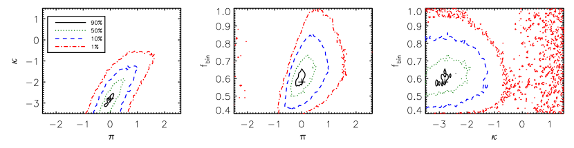
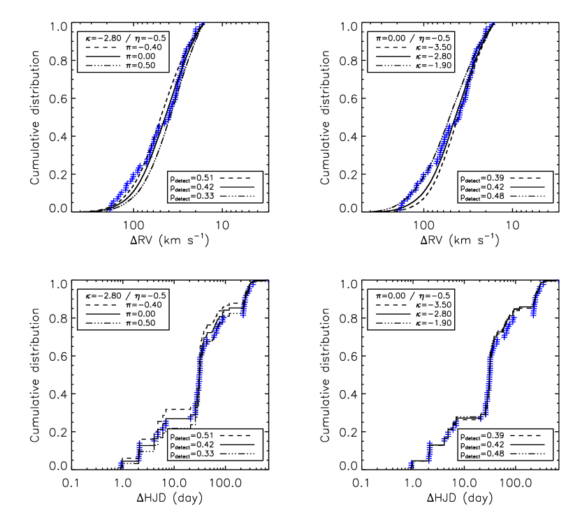
Figure 5: Projections of the global merit function, $\Xi^{\prime}$, on the pairs of planes defined by $\pi$, $\kappa$ and $f_{\rm B(true)}$. The location of the absolute maximum is indicated by a cross ($+$) and contours indicate loci of equal values in the merit function, expressed as a fraction of its absolute maximum (see inset in left-hand panel).

Figure 6: Comparison of the observed (crosses) and simulated (lines) cumulative distributions of the peak-to-peak RV amplitudes (upper panels) and of the variability timescales (lower panels). The exponent $\pi$ (period distribution) is varied in the left-hand panels, while $\kappa$ (the exponent of the mass-ratio distribution), is varied in the right-hand panels. Values of $\pi$, $\kappa$ and $\eta$ are indicated in the upper-left insets of each panel. The lower-right insets indicate the VFTS detection probability for the range of parameters specified in Table 5 and for the adopted parent distributions.

6 Summary

We have investigated the multiplicity properties of 408 B-type stars in 30 Dor, employing the multi-epoch spectroscopy from the VFTS. We find that at least 25% of the stars display significant RV variations that are large enough to potentially be the spectroscopic signature of binarity. An additional 9% of the stars display RV variations – these are either binary candidates or display intrinsic atmospheric variability.

By modelling the properties of our observations, we estimate our observational biases and constrain the intrinsic multiplicity properties of the B-type stars in 30 Dor. The binary fraction of the unevolved (i.e. dwarf/giant) stars is estimated to be $f_{\rm B(true)}$ $=$ 0.58 $\pm$ 0.11, with a flat period distribution. The uncertainties on the mass-ratio distribution are large and the best-fit distribution should be considered with caution. Nonetheless, the multiplicity properties of the B-type stars agree (within the uncertainties) with those of the O-type stars in 30 Dor. Although the B-star sample is larger, the uncertainties are greater than for the O stars, a consequence of the B stars being fainter (hence having spectroscopy with generally lower S/N). Our results indicate that the important evolutionary implications of binarity inferred for the O-star sample probably also hold for the stars born as B-type, and hence for the entire population of supernova progenitors. Comprehensive spectroscopic monitoring of the B-type sample is now required to determine the period distribution to firmly test this conclusion.

Appendix A Spatially-resolved companions

The Medusa fibres subtend 1$\aas@@fstack{\prime\prime}$2 on the sky which, at the distance of the LMC (50 kpc), is equivalent to 0.29 pc. Some of the spectra could therefore be composites of both wide binaries and/or chance line-of-sight alignments. High-quality optical imaging from the wide-field F775W mosaic of 30 Dor taken with the Hubble Space Telescope (HST) in programme GO-12499 (PI: Lennon; see Sabbi et al. 2013) includes 300 of the 403 stars (74%) with RV estimates.

We checked the available shallow and deep images for companions within 1^′′. Two of us (PLD and SdM) visually checked each of our targets for nearby companions which could have significantly contaminated the LR02 spectroscopy; notable companions/features in this context are summarised in Table 6. Although subjective, the two independent evaluations were in excellent agreement, ensuring that important companions, as resolved by HST imaging, are noted.

We detect visual companions that could contribute to the observed spectra for thirty-five of the B-star targets (i.e. 11.7 % of those with imaging available). In the context of searching for spectroscopic binaries such visual companions sample a very different range of physical separations (see e.g. Fig. 1 from Sana & Evans 2011) and they will not influence the results for the spectroscopic binary sample analysed in this paper. Even if they are physically bound, the RV amplitudes for these visual-binary systems will be below our detection threshold, and they will therefore be categorised as single using the spectroscopic criteria described in Section 3 (in the absence of other sources of RV variability). Such wide systems are unlikely to interact at any point in their evolution, and so will have no influence on our conclusions in this respect. However, to the extent that the observed spectra will be composite to some (generally small) degree, this contamination will need to be taken into account in any future atmospheric analyses of these spectra.

Table 6: B-type targets that may have a significant contribution to their FLAMES spectra from nearby companions.

VFTS	Comment
043	Elongated image - close companion
044	Elongated image - close companion
050	Star with similar mag. at 1″
068	Fainter star at $\sim$0.5″
127	Fainter star at $<$0.5″
133	Star with similar mag. at $\sim$0.5″
167	Elongated image - close companion
212	Elongated image - close companion
238	Two fainter stars, at $<$0.5″& $\sim$0.5″
276	Star with similar mag. at $\sim$0.5″
278	Crowded field, 4 fainter stars at $<$0.5″
283	Two stars with similar mag. at $\sim$0.5″
292	Three fainter stars at $<$0.5″
301	Star with similar mag. at $\sim$1″
374	Fainter star at $<$0.5″
376	Elongated image - close companion
381	Star with similar mag. at $\sim$0.5″
403	Star with similar mag. at $\sim$1″
447	Star with similar mag. at $<$0.5″
448	Star with similar mag. at $<$0.5″
461	Star with similar mag. at $<$0.5″
463	Fainter star at $<$0.5″
480	Two fainter stars at $<$0.5″
504	Star with similar mag. at $\sim$1″
548	Fainter star at $<$0.5″
553	Fainter star at $\sim$0.5″
567	Crowded field, star with similar mag. at 0.5″
584	Two fainter stars at $\sim$0.5″
632	Fainter star at 0.5″
643	Star with similar mag. at $\sim$0.5″
644	Star with similar mag. at $\sim$0.5″
662	Fainter star at $<$0.5″
712	Star with similar mag. at $<$0.5″
747	Star with similar mag. at $<$0.5″
833	Elongated image - close companion

Appendix B Accuracy of the MC method

As in Paper VIII, we estimated the accuracy of the method by applying it to synthetic data which shared the same properties as the sample of early-B dwarfs analysed in this paper. We adopted different parent distributions to generate the synthetic observations and investigated how well the method behaved in different parts of parameter space, including the region where the adopted parameters led to the best representation of the merit function. The results from these tests are reported in Table 7.

Table 7: Overview of test results from synthetic datasets. The input multiplicity parameters are given first in Cols. 2 to 4. The medians and 0.16 and 0.74 percentiles of the retrieved parameters from a set of 50 test runs are then indicated. The properties of the computed Monte Carlo grid are the same as those in Table 5.

$\Delta$RVmin	Multiplicity properties
[km s-1 ]	$f_{\rm B(true)}$	$\pi$	$\kappa$
	($f_{\rm B(true)}$ $=$ 0.70)	($\pi_{\mathrm{true}}=0.0$)	($\kappa_{\mathrm{true}}=0.0$)
16.0	0.70 [ 0.62,0.82]	$-$0.20 [$-$0.50,$+$0.20]	$-$0.40 [$-$1.00,$+$0.90]
	($f_{\rm B(true)}$ $=$ 0.70)	($\pi_{\mathrm{true}}=-0.5$)	($\kappa_{\mathrm{true}}=0.0$)
16.0	0.68 [ 0.62,0.76]	$-$0.70 [$-$1.10,$-$0.40]	$-$0.50 [$-$1.00,$+$0.60]
	($f_{\rm B(true)}$ $=$ 0.70)	($\pi_{\mathrm{true}}=0.0$)	($\kappa_{\mathrm{true}}=-2.5$)
16.0	0.68 [ 0.54,0.78]	$-$0.20 [$-$0.50,$+$0.20]	$-$2.90 [$-$3.50,$-$2.20]
	($f_{\rm B(true)}$ $=$ 0.55)	($\pi_{\mathrm{true}}=0.0$)	($\kappa_{\mathrm{true}}=-2.5$)
16.0	0.52 [ 0.42,0.64]	$-$0.20 [$-$0.60,$+$0.40]	$-$3.00 [$-$3.50,$-$2.00]