Large $\bm{N}$ non-perturbative effects in $\bm{\mathcal{N}=4}$ superconformal Chern-Simons theories

Abstract

We investigate the large $N$ instanton effects of partition functions in a class of $\mathcal{N}=4$ circular quiver Chern-Simons theories on a three-sphere. Our analysis is based on the supersymmetry localization and the Fermi-gas formalism. The resulting matrix model can be regarded as a two-parameter deformation of the ABJM matrix model, and has richer non-perturbative structures. Based on a systematic semi-classical analysis, we find analytic expressions of membrane instanton corrections. We also exactly compute the partition function for various cases and find some exact forms of worldsheet instanton corrections, which appear as quantum mechanical non-perturbative corrections in the Fermi-gas system.

1 Introduction

Over the last couple of years, many interesting features of non-perturbative effects in M-theory on $AdS_{4}$ background were discovered via the AdS/CFT correspondence. Utilizing the powerful techniques of the supersymmetry localization Pestun and so-called Fermi gas approach MP2 to the partition function of the dual CFT on $S^{3}$, now we have a very detailed understanding HMMO of the non-perturbative effects in M-theory on $AdS_{4}\times S^{7}/\mathbb{Z}_{k}$, which is holographically dual to the ABJ(M) theory ABJM ; ABJ .

It is realized that the existence of the two types of instanton effects, worldsheet instantons Cagnazzo:2009zh and membrane (D2-brane) instantons DMP2 , is necessary for the consistency of the theory. From the bulk M-theory perspective, these two types of instantons are both originating from certain configurations of M2-branes wrapping some three-cycles, but they are distinguished by the different dependences on the Planck constant $\hbar=2\pi k$ of the Fermi gas system. Membrane instantons are already visible in the semi-classical small $\hbar$-expansion of the Fermi gas, while worldsheet instanton effects are non-perturbative in $\hbar$. One can study such worldsheet instanton effects from the opposite large $\hbar$ regime, by $1/\hbar$-expansion of the matrix model associated with the Fermi gas system, which corresponds to the ordinary genus expansion of the matrix model with the string coupling given by $g_{s}=1/\hbar$ MP1 ; DMP1 ; FHM . From the viewpoint of this $g_{s}$-expansion, the membrane instantons appear as non-perturbative effects in $g_{s}$. The pole cancellation mechanism found in HMO2 is important for the consistency of these two expansions, since it guarantees that we can go smoothly from the small $\hbar$ regime to the large $\hbar$ regime. There are also additional contributions, namely the bound states of worldsheet instantons and membrane instantons HMO3 , which are hard to study from both small $\hbar$ and large $\hbar$ expansions. Fortunately, in the case of ABJ(M) theory, we have a complete understanding of the worldsheet instantons, membrane instantons, and their bound states, thanks to the relation to the (refined) topological string on local $\mathbb{P}^{1}\times\mathbb{P}^{1}$ HMMO ; HoO ; MaMo ; CGM ; GHM2 and exact results for various specific values of the parameters HMO1 ; PY ; MaMo ; HoO . (see Hatsuda:2013yua ; Grassi:2013qva for similar progress in half-BPS Wilson loop)

However, for more general 3d gauge theories with less supersymmetry, we still do not know detailed structures of the non-perturbative effects. Some progress along this direction has been made in the study of an $\mathcal{N}=4$ $U(N)$ gauge theory with $N_{f}$ fundamental and one adjoint hypermultiplets, which appears as the worldvolume theory on $N$ D2-branes in the presence of $N_{f}$ D6-branes. After applying the localization technique KWY1 ; Jafferis ; HHL1 ; Hosomichi , the partition function of this theory on $S^{3}$ is reduced to a matrix model, called the $N_{f}$ matrix model GM ; MePu . In HO , using the Fermi gas approach with the identification $\hbar=N_{f}$, the analytic forms of the first few membrane instanton corrections of this model were determined. Worldsheet instantons can also be studied, in principle, by the genus expansion of the $N_{f}$ matrix model. The genus-zero and the genus-one free energies of the $N_{f}$ matrix model were calculated in GM , but in practice the computation of the higher genus corrections is not so easy. Instead, the analytic forms of the first few worldsheet instantons were found in HO from the exact computation of the partition functions at finite $N$ up to certain high $N=N_{\text{max}}$. It turned out that the results of the membrane instantons and worldsheet instantons in the $N_{f}$ matrix model are quite different from the ABJ(M) case. In particular, the membrane instanton coefficients are given by the gamma functions of $N_{f}$ and quite different from the Gopakumar-Vafa type formula Gopakumar:1998jq in (refined) topological string, where only trigonometric functions of $\hbar$ or $1/\hbar$ appear. To understand the underlying structure better, it is desirable to study non-perturbative effects in various other models with $\mathcal{N}=4$ supersymmetries.

In this paper we study a special class of $\mathcal{N}=4$ super Chern-Simons matter theories in three dimensions Gaiotto:2008sd ; Hosomichi:2008jd : a circular quiver gauge theory with the gauge group $U(N)_{k}\times U(N)_{0}^{q-1}\times U(N)_{-k}\times U(N)_{0}^{p-1}$ and bi-fundamental hypermultiplets one by one between nearest neighboring pairs of gauge groups. The subscripts in the gauge group represent the Chern-Simons level for each factor. In this paper, we will refer to this theory as “$(p,q)$-model”. It is expected that the $(p,q)$-model is the low-energy effective theory of $N$ M2-branes probing the orbifold $(\mathbb{C}^{4}/(\mathbb{Z}_{p}\times\mathbb{Z}_{q}))/\mathbb{Z}_{k}$ Imamura:2008nn ; Imamura:2008dt , where the orbifolding action is given by (2.90), and this model is dual to M-theory on $AdS_{4}\times(S^{7}/(\mathbb{Z}_{p}\times\mathbb{Z}_{q}))/\mathbb{Z}_{k}$ through the AdS/CFT correspondence. The $(p,q)$-model can be regarded as a two-parameter deformation of the ABJM theory, hence it is expected that there is a rich non-perturbative structure in this model. For instance, the ABJM model corresponds to the $(p,q)=(1,1)$ model, while the $N_{f}$ matrix model corresponds to the $(p,q)=(1,N_{f})$ model with the Chern-Simons level $k=1$.

We will study the large $N$ instanton effects in the $(p,q)$-model by analyzing the partition function on $S^{3}$. By applying the localization method, the partition function of the $(p,q)$-model is reduced to a matrix integral KWY1 ; Jafferis ; HHL1 , which can be further studied by the Fermi gas formalism with the identification $\hbar=2\pi k$. Note that the partition function of the $(p,q)$-model is invariant under the exchange of $p$ and $q$ with fixed $k$. In the original set-up of the circular quiver gauge theory, $p,q$ and $k$ are all integers, but at the level of the partition function, we can consider an analytic continuation of the parameters $(p,q,k)$ to arbitrary real (or complex) numbers. The study of the $(p,q)$-model in the Fermi gas formalism was initiated in MN1 ; MN2 . The perturbative part of the grand potential was determined in MN1 , and in MN2 it was found that there are three types of membrane instanton corrections in the grand potential,

$$\mathcal{O}(e^{-\frac{2\mu}{p}}),\qquad\mathcal{O}(e^{-\frac{2\mu}{q}}),\qquad\mathcal{O}(e^{-\mu}),\qquad$$ (1.1)

where $\mu$ denotes the chemical potential of the Fermi gas system. These instantons contribute to the canonical partition function at large $N$ by $\mathcal{O}(e^{-\pi\sqrt{\frac{2qkN}{p}}})$, $\mathcal{O}(e^{-\pi\sqrt{\frac{2pkN}{q}}})$ and $\mathcal{O}(e^{-\pi\sqrt{\frac{pqkN}{2}}})$, respectively. The first two types of instantons are simply related by the exchange of $p$ and $q$. In this paper, to study such membrane instanton corrections we will develop a systematic method for the $\hbar$-expansion (WKB expansion) of the grand potential. Using the data of the WKB expansion, we determine the analytic form of the leading menbrane instanton correction of the first two types in (1.1) for generic $(p,q,k)$, and for the last type in (1.1) we find the analytic forms of the leading and the next-to-leading menbrane instanton corrections. Also, there are worldsheet instanton corrections of the order

$$\mathcal{O}(e^{-\frac{4\mu}{pqk}}),$$ (1.2)

which contributes to the canonical partition function by $\mathcal{O}(e^{-2\pi\sqrt{\frac{2N}{pqk}}})$ at large $N$. From the exact computation of the partition functions at finite $N$, we find the analytic form of the leading worldsheet instanton correction for generic $(p,q,k)$. We will see that our results of the menbrane instantons and worldsheet instantons satisfy the pole cancellation conditions as expected, and they also correctly reproduce the known results of the ABJM model and the $N_{f}$ matrix model by taking the appropriate limits of the parameters $(p,q,k)$. Study of the bound state corrections in the $(p,q)$ model is beyond the scope of this paper.

This paper is organized as follows. In section 2, after introducing the Fermi gas formalism of the $(p,q)$-model, we explain our method of the WKB expansion of the grand potential and our algorithm for the exact computation of the partition functions. We also comment on the instanton effects in the $(p,q)$ model from the dual gravity viewpoint. Then, we present the results for the $(p,q)=(1,q)$ case in section 3, and the results for the general $(p,q)$ case in section 4. In the both cases, we find the analytic forms of the first few membrane instanton and worldsheet instanton corrections. In section 5, we consider some interesting cases with the special values of $(p,q)$. We discuss that the grand potential for $(p,q)=(1,-1)$ is captured by the refined topological string on a resolved conifold. We also find an exact closed form expression of the grand partition function of the $(p,q)=(2,2)$ model at $k=1$. Section 6 is devoted to conclusions and discussions. In appendices A to F, we summarize some useful results used in the main text.

2 Fermi-gas approach to $\mathcal{N}=4$ quiver CS matrix model

In this section we introduce the ideal Fermi gas formalism of the $(p,q)$-model and discuss how to extract information on the large $N$ non-perturbative effects in the corresponding M-theory dual.

2.1 From matrix model to Fermi-gas

It is known that the partition function of the $(p,q)$-model on $S^{3}$ is reduced to the matrix integral thanks to the supersymmetry localization KWY1 ; Jafferis ; HHL1 ,

$$Z(N,k)=\frac{1}{(N!)^{p+q}}\int\prod_{a=1}^{p+q}\frac{d^{N}\mu^{(a)}}{(2\pi)^{N}}\exp{\Bigl{[}\frac{ik}{4\pi}\sum_{j=1}^{N}\left((\mu_{j}^{(1)})^{2}-(\mu_{j}^{(q+1)})^{2}\right)\Bigr{]}}\prod_{a=1}^{p+q}\frac{\prod_{i<j}\Bigl{[}2\sinh{\frac{\mu_{i}^{(a)}-\mu_{j}^{(a)}}{2}}\Bigr{]}^{2}}{\prod_{i,j}2\cosh{\frac{\mu_{i}^{(a)}-\mu_{j}^{(a+1)}}{2}}},$$ (2.1)

where $\mu^{(p+q+1)}=\mu^{(1)}$. This matrix model can be further simplified by using the ideal Fermi gas approach MP2 . To be self-contained, here we briefly review the derivation of the Fermi gas representation. First, by using the Cauchy determinant formula

$$\frac{\prod_{i<j}\Bigl{[}2\sinh{\frac{x_{i}-x_{j}}{2}}\Bigr{]}\Bigl{[}2\sinh{\frac{y_{i}-y_{j}}{2}}\Bigr{]}}{\prod_{i,j}2\cosh{\frac{x_{i}-y_{j}}{2}}}=\sum_{\sigma}(-1)^{\sigma}\prod_{j}\frac{1}{2\cosh{\frac{x_{j}-y_{\sigma(j)}}{2}}},$$

we rewrite the partition function as

$$Z(N,k) = \frac{1}{N!}\sum_{\sigma}(-1)^{\sigma}\int\prod_{a=1}^{p+q}\frac{d^{N}\mu^{(a)}}{(2\pi k)^{N}}\exp{\Bigl{[}\frac{i}{4\pi k}\sum_{j=1}^{N}\left((\mu_{j}^{(1)})^{2}-(\mu_{j}^{(q+1)})^{2}\right)\Bigr{]}}$$ (2.2)

$$\times\prod_{a=1}^{p+q-1}\Biggl{[}\prod_{j=1}^{N}\frac{1}{2\cosh{\frac{\mu_{j}^{(a)}-\mu_{j}^{(a+1)}}{2k}}}\Biggr{]}\times\prod_{j=1}^{N}\frac{1}{2\cosh{\frac{\mu_{j}^{(p+q)}-\mu_{\sigma(j)}^{(1)}}{2k}}}$$

$$= \frac{1}{N!}\sum_{\sigma}(-1)^{\sigma}\int d^{N}\mu^{(1)}\prod_{j=1}^{N}\rho(\mu_{j}^{(1)},\mu_{\sigma(j)}^{(1)}),$$

where we have trivialized most of the permutations and the function $\rho$ is given by

$$\rho(x,y)=\frac{1}{2\pi k}\int\prod_{a=2}^{p+q}\frac{d\mu^{(a)}}{2\pi k}\frac{e^{\frac{i}{4\pi k}x^{2}-\frac{ik}{4\pi}(\mu^{(q+1)})^{2}}}{2\cosh{\frac{x-\mu^{(2)}}{2k}}}\prod_{a=2}^{p+q-1}\Biggl{[}\frac{1}{2\cosh{\frac{\mu^{(a)}-\mu^{(a+1)}}{2k}}}\Biggr{]}\frac{1}{2\cosh{\frac{\mu^{(p+q)}-y}{2k}}}.$$ (2.3)

Thus we can regard the partition function as an ideal Fermi gas system with the density matrix $\rho(x,y)$. The expression of $\rho$ is further simplified if we regard $\rho$ as the matrix element of the quantum mechanical operator $\hat{\rho}(\hat{Q},\hat{P})$ with $(\hat{Q},\hat{P})$ satisfying the canonical commutation relation

$$[\hat{Q},\hat{P}]=i\hbar,\quad\hbar=2\pi k.$$ (2.4)

Then, the density matrix $\rho(x,y)$ is understood as

$$\rho(x,y)=\frac{1}{\hbar}\langle x|\hat{\rho}|y\rangle,$$ (2.5)

where

$$\hat{\rho}(\hat{Q},\hat{P})=e^{\frac{i}{2\hbar}\hat{Q}^{2}}\frac{1}{\left(2\cosh{\frac{\hat{P}}{2}}\right)^{q}}e^{-\frac{i}{2\hbar}\hat{Q}^{2}}\frac{1}{\left(2\cosh{\frac{\hat{P}}{2}}\right)^{p}}.$$ (2.6)

Using the convenient formula $e^{\frac{i\hat{Q}^{2}}{2\hbar}}f(\hat{P})e^{-\frac{i\hat{Q}^{2}}{2\hbar}}=f(\hat{P}-\hat{Q})$ and $e^{\frac{i\hat{P}^{2}}{2\hbar}}g(\hat{Q})e^{-\frac{i\hat{P}^{2}}{2\hbar}}=g(\hat{Q}+\hat{P})$, we find

$$\hat{\rho}(\hat{Q},\hat{P})=e^{-\frac{i}{2\hbar}\hat{P}^{2}}\frac{1}{\left(2\cosh{\frac{\hat{Q}}{2}}\right)^{q}}\frac{1}{\left(2\cosh{\frac{\hat{P}}{2}}\right)^{p}}e^{\frac{i}{2\hbar}\hat{P}^{2}}.$$ (2.7)

If we perform the similarity transformation

$$\hat{\rho}\rightarrow\Bigl{(}2\cosh{\frac{\hat{Q}}{2}}\Bigr{)}^{q/2}e^{\frac{i}{2\hbar}\hat{P}^{2}}\hat{\rho}e^{-\frac{i}{2\hbar}\hat{P}^{2}}\Bigl{(}2\cosh{\frac{\hat{Q}}{2}}\Bigr{)}^{-q/2},$$ (2.8)

then the operator $\hat{\rho}$ is simplified to

$$\hat{\rho}(\hat{Q},\hat{P})=\frac{1}{\left(2\cosh{\frac{\hat{Q}}{2}}\right)^{q/2}}\frac{1}{\left(2\cosh{\frac{\hat{P}}{2}}\right)^{p}}\frac{1}{\left(2\cosh{\frac{\hat{Q}}{2}}\right)^{q/2}}.$$ (2.9)

Note that the partition function is invariant under any similarity transformations. In the coordinate representation, the density operator (2.9) is expressed by

$$\rho(x_{1},x_{2})=\frac{1}{4\pi^{2}k}\frac{1}{\left(2\cosh\frac{x_{1}}{2}\right)^{q/2}}\frac{1}{\left(2\cosh\frac{x_{2}}{2}\right)^{q/2}}\operatorname{B}\left(\frac{p}{2}+\frac{i(x_{1}-x_{2})}{2\pi k},\frac{p}{2}-\frac{i(x_{1}-x_{2})}{2\pi k}\right),$$ (2.10)

where $\operatorname{B}(x,y)=\Gamma(x)\Gamma(y)/\Gamma(x+y)$ is the Euler beta function. For $p\in\mathbb{Z}_{>0}$, one can show that this expression reduces to the one in MN3 . In particular, for $p=q=1$, it reduces to the density matrix in the ABJM Fermi-gas as expected. Also, the case for $(p,q,k)=(1,2,1)$ gives the density matrix for the $U(N)_{2}\times U(N+1)_{-2}$ ABJ theory HoO ; Honda ; AHS as explained in HO . Note that the partition function is invariant under the exchange $p\leftrightarrow q$. This invariance is no longer manifest in the coordinate representation (2.10).

2.2 Grand canonical formalism

As was proposed in MP2 , a useful way to treat this system is to introduce the grand canonical partition function

$$\Xi(\kappa,k)=1+\sum_{N=1}^{\infty}\kappa^{N}Z(N,k),\quad\kappa=e^{\mu},$$ (2.11)

where $\kappa$ and $\mu$ is the fugacity and the chemical potential, respectively. We can return to the canonical partition function by

$$Z(N,k)=\frac{1}{2\pi i}\oint\frac{d\kappa}{\kappa^{N+1}}\Xi(\kappa,k).$$ (2.12)

The grand partition function is given by the Fredholm determinant

$$\Xi(\kappa,k)=\det(1+\kappa\hat{\rho})=\prod_{n=0}^{\infty}(1+\kappa\lambda_{n}),$$ (2.13)

where $\lambda_{n}$ ($n\in\mathbb{Z}_{\geq 0}$) are the eigenvalues of $\hat{\rho}$. The spectral problem for this system is represented by the Fredholm integral equation:

$$\int_{-\infty}^{\infty}dx^{\prime}\,\rho(x,x^{\prime})\phi_{n}(x^{\prime})=\lambda_{n}\phi_{n}(x).$$ (2.14)

It is easy to see that the grand potential is given by

$$\mathcal{J}(\kappa,k)=\log\Xi(\kappa,k)=-\sum_{\ell=1}^{\infty}\frac{(-\kappa)^{\ell}}{\ell}\zeta_{\rho}(\ell),$$ (2.15)

where $\zeta_{\rho}(s)$ is a spectral zeta function defined by

$$\zeta_{\rho}(s)=\operatorname{Tr}\hat{\rho}^{s}=\sum_{n=0}^{\infty}\lambda_{n}^{s}.$$ (2.16)

In particular, for $s=\ell\in\mathbb{Z}_{>0}$, it can be computed directly by the multi-integral

$$\zeta_{\rho}(\ell)=\int_{-\infty}^{\infty}\!\cdots\!\int_{-\infty}^{\infty}dx_{1}\cdots dx_{\ell}\;\rho(x_{1},x_{2})\cdots\rho(x_{\ell},x_{1}).$$ (2.17)

As in Hatsuda ; MarinoReview , it is convenient to rewrite (2.15) as the following Mellin-Barnes like integral:

$$\mathcal{J}(\mu,k)=-\int_{c-i\infty}^{c+i\infty}\frac{ds}{2\pi i}\Gamma(s)\Gamma(-s)\zeta_{\rho}(s)e^{s\mu}.$$ (2.18)

The constant $c$ must be taken such that $0<c<1$. Depending on the sign of $\mu$, one can deform the integral contour in the following ways. For $\mu<0$, one can deform the countour by adding an infinite semi-circle $C_{+}$ as shown in figure 1. Then the integral can be evaluated by the sum of the residues over all the poles in the region $\operatorname{Re}s>c$. As shown in Hatsuda , the spectral zeta function $\zeta_{\rho}(s)$ does not have any poles in the region $\operatorname{Re}s>0$. If $0<c<1$, the poles inside the contour are located at $s=\ell$ ($\ell\in\mathbb{Z}_{>0}$), coming solely from the factor $\Gamma(-s)$, and thus we precisely recover the sum (2.15). On the other hand, for $\mu>0$ one can deform the contour by adding the opposite semi-circle $C_{-}$ as in figure 1. In this case, one needs the information of the poles in the region $\operatorname{Re}s<c$, in which $\zeta_{\rho}(s)$ may have non-trivial poles, and the problem is highly non-trivial for general $k$. As we will see below, in the semi-classical analysis, we can find all the poles of $\zeta_{\rho}(s)$ and compute the large $\mu$ expansion systematically.

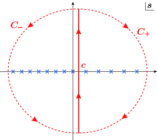
Figure 1: One can deform the integration contour in (2.18) into a closed path by adding an infinite semi-circle $C_{+}$ ($C_{-}$) for $\mu<0$ ($\mu>0)$. We schematically show the poles of the integrand.

2.3 Classical approximation

Since the ideal Fermi gas formalism provides us with the quantum mechanical description of the system, it is useful to consider the semi-classical $\hbar$-expansion, or equivalently the small-$k$ expansion

$$\mathcal{J}_{\text{WKB}}(\mu,k)=\frac{1}{k}\sum_{n=0}^{\infty}k^{2n}\mathcal{J}^{(n)}(\mu),$$ (2.19)

where $\mathcal{J}_{\text{WKB}}$ is expected to approximate the exact grand potential $\mathcal{J}$ up to exponentially suppressed corrections in $\hbar$. Let us start with the classical approximation, namely $\mathcal{O}(k^{-1})$. Note that the large $\mu$ expansion in this limit has already been analyzed in MN2 . Here, we simply re-derive their result by using the Mellin-Barnes integral (2.18). In the classical approximation, the density operator is given by

$$\rho_{\text{cl}}=\frac{1}{\bigl{(}2\cosh\frac{Q}{2}\bigr{)}^{q}}\frac{1}{\bigl{(}2\cosh\frac{P}{2}\bigr{)}^{p}}.$$ (2.20)

Then, the spectral zeta function can be easily computed by the phase space integral

$$\zeta_{\rho}^{(0)}(s)=\int_{-\infty}^{\infty}\frac{dQdP}{4\pi^{2}}\frac{1}{\bigl{(}2\cosh\frac{Q}{2}\bigr{)}^{qs}}\frac{1}{\bigl{(}2\cosh\frac{P}{2}\bigr{)}^{ps}}=\frac{1}{4\pi^{2}}\frac{\Gamma^{2}(\frac{ps}{2})\Gamma^{2}(\frac{qs}{2})}{\Gamma(ps)\Gamma(qs)}.$$ (2.21)

We would like to know the large $\mu$ expansion of the classical grand potential. Plugging (2.21) into (2.18), one obtains

$$\mathcal{J}^{(0)}(\mu)=-\frac{1}{4\pi^{2}}\int_{c-i\infty}^{c+i\infty}\frac{ds}{2\pi i}\Gamma(s)\Gamma(-s)\frac{\Gamma^{2}(\frac{ps}{2})\Gamma^{2}(\frac{qs}{2})}{\Gamma(ps)\Gamma(qs)}e^{s\mu}.$$ (2.22)

If we take the integral contour $\mathcal{C}_{-}$ in fig. 1, then the leading large $\mu$ contribution comes from the residue at $s=0$:

$$-\frac{1}{4\pi^{2}}\mathop{\rm Res}\limits_{s=0}\Gamma(s)\Gamma(-s)\frac{\Gamma^{2}(\frac{ps}{2})\Gamma^{2}(\frac{qs}{2})}{\Gamma(ps)\Gamma(qs)}e^{s\mu}=\frac{2}{3\pi^{2}pq}\mu^{3}+\frac{4-p^{2}-q^{2}}{6pq}\mu+\frac{p^{3}+q^{3}}{\pi^{2}pq}\zeta(3).$$ (2.23)

In the region $\operatorname{Re}s<0$, the integrand of (2.22) has the following three types of poles:

$$s=-\frac{2n}{p},\qquad s=-\frac{2n}{q},\qquad s=-n,\qquad(n\in\mathbb{Z}_{>0}).$$ (2.24)

The residue at $s=-2n/p$ is given by

$$-\frac{1}{4\pi^{2}}\mathop{\rm Res}\limits_{s=-2n/p}\Gamma(s)\Gamma(-s)\frac{\Gamma^{2}(\frac{ps}{2})\Gamma^{2}(\frac{qs}{2})}{\Gamma(ps)\Gamma(qs)}e^{s\mu}=\frac{1}{2\pi n}\binom{2n}{n}\csc\left(\frac{2\pi n}{p}\right)\frac{\Gamma^{2}(-\frac{nq}{p})}{\Gamma(-\frac{2nq}{p})}e^{-\frac{2n\mu}{p}}.$$ (2.25)

The residue at $s=-2n/q$ is obtained by exchanging $p$ and $q$. The residue at $s=-n$ is also computed as

$$-\frac{1}{4\pi^{2}}\mathop{\rm Res}\limits_{s=-n}\Gamma(s)\Gamma(-s)\frac{\Gamma^{2}(\frac{ps}{2})\Gamma^{2}(\frac{qs}{2})}{\Gamma(ps)\Gamma(qs)}e^{s\mu}=\frac{(-1)^{n-1}}{4\pi^{2}n}\frac{\Gamma^{2}(-\frac{np}{2})}{\Gamma(-np)}\frac{\Gamma^{2}(-\frac{nq}{2})}{\Gamma(-nq)}e^{-n\mu}.$$ (2.26)

We conclude that the large $\mu$ expansion of the classical grand potential takes the form

$$\mathcal{J}^{(0)}(\mu)=\frac{2}{3\pi^{2}pq}\mu^{3}+\frac{4-p^{2}-q^{2}}{6pq}\mu+\frac{p^{3}+q^{3}}{\pi^{2}pq}\zeta(3)+\mathcal{J}^{(0)}_{\text{M2,I}}(\mu)+\mathcal{J}^{(0)}_{\text{M2,II}}(\mu)+\mathcal{J}^{(0)}_{\text{M2,III}}(\mu),$$ (2.27)

where

$$\mathcal{J}^{(0)}_{\text{M2,I}}(\mu) =\sum_{n=1}^{\infty}\frac{1}{2\pi n}\binom{2n}{n}\csc\left(\frac{2\pi n}{p}\right)\frac{\Gamma^{2}(-\frac{nq}{p})}{\Gamma(-\frac{2nq}{p})}e^{-\frac{2n\mu}{p}},$$ (2.28)

$$\mathcal{J}^{(0)}_{\text{M2,II}}(\mu) =\sum_{n=1}^{\infty}\frac{1}{2\pi n}\binom{2n}{n}\csc\left(\frac{2\pi n}{q}\right)\frac{\Gamma^{2}(-\frac{np}{q})}{\Gamma(-\frac{2np}{q})}e^{-\frac{2n\mu}{q}},$$

$$\mathcal{J}^{(0)}_{\text{M2,III}}(\mu) =\sum_{n=1}^{\infty}\frac{(-1)^{n-1}}{4\pi^{2}n}\frac{\Gamma^{2}(-\frac{np}{2})}{\Gamma(-np)}\frac{\Gamma^{2}(-\frac{nq}{2})}{\Gamma(-nq)}e^{-n\mu}.$$

These expressions reproduce the results in MN2 .

2.4 Semi-classical analysis

Let us proceed to the quantum corrections to the grand potential. To compute the quantum correction to $\zeta_{\rho}(s)$, we use the Wigner transform, as in MP2 . For a given operator $\hat{A}$, the Wigner transform is defined by

$$A_{\text{W}}(Q,P)=\int_{-\infty}^{\infty}\frac{dQ^{\prime}}{\hbar}\,e^{\frac{iPQ^{\prime}}{\hbar}}\left\langle Q-\frac{Q^{\prime}}{2}\right|\hat{A}\left|Q+\frac{Q^{\prime}}{2}\right\rangle.$$ (2.29)

The trace of $\hat{A}$ is then given by the phase space integral

$$\operatorname{Tr}\hat{A}=\int_{-\infty}^{\infty}\frac{dQdP}{2\pi\hbar}A_{\text{W}}(Q,P).$$ (2.30)

Let us apply the Wigner transform to the inverse of the density operator

$$\hat{\mathcal{O}}=\hat{\rho}^{-1}=\biggl{(}2\cosh\frac{\hat{Q}}{2}\biggr{)}^{q/2}\biggl{(}2\cosh\frac{\hat{P}}{2}\biggr{)}^{p}\biggl{(}2\cosh\frac{\hat{Q}}{2}\biggr{)}^{q/2}.$$ (2.31)

As shown in appendix A, the Wigner transform of $\hat{\mathcal{O}}$ is given by

$$\mathcal{O}_{\text{W}}(Q,P)=\biggl{(}4\cosh^{2}\frac{Q}{2}-4\sin^{2}\frac{\pi k\partial_{P}}{2}\biggr{)}^{q/2}\biggl{(}2\cosh\frac{P}{2}\biggr{)}^{p}.$$ (2.32)

Using this result, one can easily compute the WKB expansion of $\mathcal{O}_{\text{W}}(Q,P)$ up to any order. We would like to compute the spectral trace

$$\zeta_{\rho}(s)=\operatorname{Tr}\hat{\rho}^{s}=\operatorname{Tr}\hat{\mathcal{O}}^{-s}.$$ (2.33)

Expanding $\hat{\mathcal{O}}^{-s}$ around $\mathcal{O}_{\text{W}}$ as in MP2 ; Hatsuda , the Wigner transform of $\hat{\mathcal{O}}^{-s}$ is computed by

$$(\hat{\mathcal{O}}^{-s})_{\text{W}}=\sum_{r=0}^{\infty}\frac{(-1)^{r}(s)_{r}}{r!}\mathcal{O}_{\text{W}}^{-s-r}[(\hat{\mathcal{O}}-\mathcal{O}_{\text{W}})^{r}]_{\text{W}},$$ (2.34)

where $(s)_{r}$ is the Pochhammer symbol. To compute the summand in (2.34), one needs the Wigner transform of operator products. The Wigner transform of a product of two operators is computed by

$$(\hat{A}\cdot\hat{B})_{\text{W}}=A_{\text{W}}\star B_{\text{W}},$$ (2.35)

where the Moyal product $\star$ is defined by

$$A\star B :=A(x,p)\exp\left[\frac{{\rm i}\hbar}{2}(\stackrel{{\scriptstyle\leftarrow}}{{\partial}}_{x}\stackrel{{\scriptstyle\rightarrow}}{{\partial}}_{p}-\stackrel{{\scriptstyle\leftarrow}}{{\partial}}_{p}\stackrel{{\scriptstyle\rightarrow}}{{\partial}}_{x})\right]B(x,p)$$ (2.36)

$$=\sum_{n=0}^{\infty}\sum_{m=0}^{n}(-1)^{m}\binom{n}{m}\frac{1}{n!}\left(\frac{{\rm i}\hbar}{2}\right)^{n}\partial_{x}^{m}\partial_{p}^{n-m}A(x,p)\partial_{p}^{m}\partial_{x}^{n-m}B(x,p).$$

In this way, one can compute $\operatorname{Tr}\hat{\mathcal{O}}^{-s}$ up to any desired order, in principle. However, the integral appearing in (2.34) for general $s$ is complicated and hard to evaluate. Practically, it is sufficient to compute it for $s\in\mathbb{Z}_{>0}$. Here, we use an interesting idea in MN2 . The quantum correction $\mathcal{J}^{(n)}(\mu)$ can be constructed by acting a non-trivial differential operator on the classical one:

$$\mathcal{J}^{(n)}(\mu)=\mathcal{D}^{(n)}\mathcal{J}^{(0)}(\mu),\qquad(n=1,2,\dots),$$ (2.37)

where $\mathcal{D}^{(n)}$ is a differential operator of $\mu$. Its explicit form up to $n=2$ was computed in MN2 . An efficient way to fix this differential operator is as follows. We first compute the expansion of $\mathcal{J}^{(n)}(\kappa)$ around $\kappa=0$. This can be done by using the formula (2.34) for $s\in\mathbb{Z}_{>0}$. Taking an ansatz of the form of $\mathcal{D}^{(n)}$, we try to fix unknown parameters to match the first several coefficients of $\mathcal{J}^{(n)}(\kappa)$. If the ansatz is correct, the obtained result must reproduce higher order coefficients. In this way, one can verify the obtained operator up to any desired order. Using this method, we have indeed fixed the differential operator up to $n=17$. The result up to $n=4$ is given in appendix B.

Using this method, we finally find that the semi-classical grand potential has the following large $\mu$ expansion

$$\mathcal{J}_{\text{WKB}}(\mu,k)=\mathcal{J}_{\rm pert}(\mu,k)+\mathcal{J}_{\text{M2,I}}(\mu,k)+\mathcal{J}_{\text{M2,II}}(\mu,k)+\mathcal{J}_{\text{M2,III}}(\mu,k),$$ (2.38)

where $\mathcal{J}_{\rm pert}(\mu,k)$ is the perturbative grand potential given by

$$\mathcal{J}_{\rm pert}(\mu,k)=\frac{C_{p,q}(k)}{3}\mu^{3}+B_{p,q}(k)\mu+A_{p,q}(k),$$ (2.39)

with

$$C_{p,q}(k)=\frac{2}{\pi^{2}pqk},\qquad B_{p,q}(k)=\frac{4-p^{2}-q^{2}}{6pqk}+\frac{pqk}{24}.$$ (2.40)

The constant part $A_{p,q}(k)$ is a complicated function of $k$, whose exact form was conjectured in MN1

$$A_{p,q}(k)=\frac{1}{2}\left(p^{2}A_{\text{c}}(qk)+q^{2}A_{\text{c}}(pk)\right),$$ (2.41)

where $A_{\text{c}}(k)$ is given by HO (see also KEK )

$$A_{\text{c}}(k)=\frac{2\zeta(3)}{\pi^{2}k}\left(1-\frac{k^{3}}{16}\right)+\frac{k^{2}}{\pi^{2}}\int_{0}^{\infty}dx\frac{x}{e^{kx}-1}\log(1-e^{-2x}).$$ (2.42)

There are three types of exponentially suppressed corrections with the following forms

$$\mathcal{J}_{\text{M2,I}}(\mu,k) =\sum_{n=1}^{\infty}\alpha_{n}(p,q,k)e^{-\frac{2n\mu}{p}},\qquad\mathcal{J}_{\text{M2,II}}(\mu,k)=\sum_{n=1}^{\infty}\alpha_{n}(q,p,k)e^{-\frac{2n\mu}{q}},$$ (2.43)

$$\mathcal{J}_{\text{M2,III}}(\mu,k) =\sum_{n=1}^{\infty}\beta_{n}(p,q,k)e^{-n\mu}.$$

Note that $\alpha_{n}(p,q,k)$ is not symmetric in $p$ and $q$, while $\beta_{n}(p,q,k)$ is symmetric (namely, $\alpha_{n}(p,q,k)\neq\alpha_{n}(q,p,k)$, $\beta_{n}(p,q,k)=\beta_{n}(q,p,k)$). Our task is to fix these coefficients.

In the later analysis, it is convenient to introduce a function $D(s,p,q,k)$ by

$$\mathcal{D}(e^{s\mu})=D(s,p,q,k)e^{s\mu},$$ (2.44)

where $\mathcal{D}$ is a generating function of $\mathcal{D}^{(n)}$,

$$\mathcal{D}=1+\sum_{n=1}^{\infty}k^{2n}\mathcal{D}^{(n)}.$$ (2.45)

The definition (2.44) means that $D(s,p,q,k)$ is obtained by replacing $\partial_{\mu}$ in $\mathcal{D}$ by $s$. Then, the WKB expansion of the spectral zeta function is simply given by

$$\zeta_{\text{WKB}}(s)=\frac{\zeta_{\rho}^{(0)}(s)}{k}D(s,p,q,k),$$ (2.46)

where the classical part $\zeta_{\rho}^{(0)}(s)$ is given by (2.21). Also, the membrane instanton coefficients in (2.43) are generically given by

$$\alpha_{n}(p,q,k)=\frac{\alpha_{n}^{(0)}(p,q)}{k}D\left(-\frac{2n}{p},p,q,k\right),\quad\beta_{n}(p,q,k)=\frac{\beta_{n}^{(0)}(p,q)}{k}D\left(-n,p,q,k\right),$$ (2.47)

where $\alpha_{n}^{(0)}(p,q)$ and $\beta_{n}^{(0)}(p,q)$ are the classical parts in (2.28):

$$\alpha_{n}^{(0)}(p,q)=\frac{1}{2\pi n}\binom{2n}{n}\csc\left(\frac{2\pi n}{p}\right)\frac{\Gamma^{2}(-\frac{nq}{p})}{\Gamma(-\frac{2nq}{p})},\quad\beta_{n}^{(0)}(p,q)=\frac{(-1)^{n-1}}{4\pi^{2}n}\frac{\Gamma^{2}(-\frac{np}{2})}{\Gamma(-np)}\frac{\Gamma^{2}(-\frac{nq}{2})}{\Gamma(-nq)}.$$ (2.48)

Thus our goal is to determine $D(-2n/p,p,q,k)$ and $D(-n,p,q,k)$. It is useful to notice the following symmetric property:

$$D(s,p,q,k)=D(-s,-p,-q,k).$$ (2.49)

One can show this by using $\left.\hat{\rho}\right|_{p\rightarrow-p,q\rightarrow-q}=\hat{\rho}^{-1}$ and $\zeta_{\rho^{-1}}(-s)=\zeta_{\rho}(s)$.

2.5 TBA approach

There is another approach to compute the grand potential by using the so-called TBA equations. In CM , the semi-classical expansion of the ABJM Fermi-gas was computed in this approach. In the present situation, for $p=1,2$, we can use this method. For $p=1$, the density matrix is given by

$$\left.\rho(x_{1},x_{2})\right|_{p=1}=\frac{1}{2\pi k}\frac{e^{-\frac{1}{2}U(x_{1})-\frac{1}{2}U(x_{2})}}{2\cosh\left(\frac{x_{1}-x_{2}}{2k}\right)},\quad{\rm with}\ U(x)=q\log\left[2\cosh\frac{x}{2}\right].$$ (2.50)

The kernel (2.50) has the same form as the one in Zamolodchikov , and one can immediately use the result there. The functional equations are given by

$$R_{+}\left(x+\frac{\pi ik}{2}\right)R_{+}\left(x-\frac{\pi ik}{2}\right)\exp\left[U\left(x+\frac{\pi ik}{2}\right)+U\left(x-\frac{\pi ik}{2}\right)\right] =1+\eta^{2}(x),$$ (2.51)

$$\eta\left(x+\frac{\pi ik}{2}\right)+\eta\left(x-\frac{\pi ik}{2}\right) =-\kappa R_{+}(x),$$

and

$$\frac{R_{-}(x+\frac{\pi ik}{2})}{R_{+}(x+\frac{\pi ik}{2})}-\frac{R_{-}(x-\frac{\pi ik}{2})}{R_{+}(x-\frac{\pi ik}{2})}=2ik\partial_{x}\arctan\eta(x).$$ (2.52)

The grand potential is computed by

$$\left.\partial_{\kappa}\mathcal{J}(\kappa,k)\right|_{p=1}=\frac{1}{4\pi k}\int_{-\infty}^{\infty}dx(R_{+}(x)+R_{-}(x)),$$ (2.53)

where an integration constant is fixed by the condition $\mathcal{J}(\kappa=0,k)=0$.

For $p=2$, the density matrix is

$$\left.\rho(x_{1},x_{2})\right|_{p=2}=\frac{1}{4\pi^{2}k}\frac{1}{\left(2\cosh\frac{x_{1}}{2}\right)^{q/2}}\frac{1}{\left(2\cosh\frac{x_{2}}{2}\right)^{q/2}}\frac{\frac{x_{1}-x_{2}}{2k}}{\sinh\frac{x_{1}-x_{2}}{2k}}.$$ (2.54)

In this case, the density matrix is different from the one in Zamolodchikov . Nevertheless, as explained in appendix C, we find the following functional equations determining the grand potential for $p=2$ in a similar way to the $p=1$ case,

$$\xi(x+\pi ik)\xi(x-\pi ik) =\eta^{2}(x)-1,$$ (2.55)

$$\eta(x+\pi ik)+\eta(x-\pi ik) =2\xi(x)\cosh 2r(x),$$

$$\frac{w(x+\pi ik)}{\xi(x+\pi ik)}-\frac{w(x-\pi ik)}{\xi(x-\pi ik)} =2i\partial_{x}\operatorname{arccoth}\eta(x),$$

where $\xi(x)$, $\eta(x)$ and $w(x)$ are unknown functions, and $r(x)$ and $t(x)$ are given by

$$r(x)=\operatorname{arcsinh}\sqrt{\frac{t(x)}{2}},\qquad t(x)=\frac{\kappa}{2(2\cosh\frac{x}{2})^{q}}.$$ (2.56)

The grand potential is then given by

$$\left.\partial_{\kappa}\mathcal{J}(\kappa,k)\right|_{p=2}=\frac{1}{\pi\kappa}\int_{-\infty}^{\infty}dx\,w(x)\sinh^{2}r(x).$$ (2.57)

The functional equations (2.51), (2.52) and (2.55) can be solved systematically around $k=0$. Therefore one can compute the WKB expansion of the grand potential.

2.6 Non-perturbative corrections: worldsheet instantons

So far, we have considered the semi-classical analysis, which is perturbative in the sense of $\hbar$. As explained in MP2 ; KM , the grand potential receives quantum mechanical non-perturbative corrections in $k$. These non-perturbative corrections are caused by the worldsheet instantons in the dual string/M-theory and invisible in the semi-classical analysis. In the case of ABJM Fermi-gas, fortunately these corrections can be predicted with the help of the topological string on local $\mathbb{P}^{1}\times\mathbb{P}^{1}$. Interestingly, for some special cases, the Fermi-gas system is related to a quantum mechanical system associated with the topological string GHM1 on certain CY, as will be seen later. In these cases, it will be possible to predict the worldsheet instanton correction, as in the ABJM Fermi-gas. However, in general, we do not know such a connection, and do not have a systematic treatment of these corrections so far. One approach to compute them is to consider the matrix model computation in the ’t Hooft limit, as was performed in DMP1 for the ABJM matrix model. In appendix D, we compute the planar free energy of the $(1,q)$ model and find the worldsheet instanton effect in the planar limit.

Following the argument in MP2 ; KM , one can estimate an order of such a non-perturbative correction. Let us consider the classical Fermi surface with energy $E$:

$$H(P,Q)=p\log\left(2\cosh\frac{P}{2}\right)+q\log\left(2\cosh\frac{Q}{2}\right)=E.$$ (2.58)

This gives an algebraic curve in the phase space. By rescaling $P=pP^{\prime},\ Q=qQ^{\prime}$, this expression becomes

$$p\log{\left(2\cosh{\frac{P^{\prime}}{2p}}\right)}+q\log{\left(2\cosh{\frac{Q^{\prime}}{2q}}\right)}=E.$$ (2.59)

In the large $E$ limit, we can approximate the Fermi surface as

$$H(P^{\prime},Q^{\prime})=E\simeq\log{\left(2\cosh{\frac{P^{\prime}}{2}}\right)}+\log{\left(2\cosh{\frac{Q^{\prime}}{2}}\right)},$$ (2.60)

up to exponentially suppressed correction. This approximated Hamiltonian leads to the equations of motion

$$\dot{Q}^{\prime}=\frac{\partial H}{\partial P^{\prime}}=\frac{1}{2}\tanh{\frac{P^{\prime}}{2}},\quad\dot{P}^{\prime}=-\frac{\partial H}{\partial Q^{\prime}}=-\frac{1}{2}\tanh{\frac{Q^{\prime}}{2}}.$$ (2.61)

On the equi-energy orbit $H(P^{\prime},Q^{\prime})=E$, $\dot{Q}^{\prime}$ becomes

$$\dot{Q}^{\prime}=\frac{1}{2}\sqrt{1-16\cosh^{2}{\frac{Q^{\prime}}{2}}e^{-2E}}.$$ (2.62)

The solution of this equation of motion is given by

$$\tanh{\frac{Q^{\prime}}{2}}=m\operatorname{sn}\left(\frac{t}{4},m\right),$$ (2.63)

where $\operatorname{sn}(u,m)$ is the Jacobi’s elliptic sine function and $m^{2}=1-16e^{-2E}$. As the function of $t$, this has the real period $\omega_{1}$ and the imaginary period $\omega_{2}$,

$$\omega_{1}=16\mathbf{K}(m),\quad\omega_{2}=8i\mathbf{K}(m^{\prime}),$$ (2.64)

where $\mathbf{K}(m)$ is the complete elliptic integral of the first kind and $m^{\prime 2}=1-m^{2}$. Now we consider the complexified Fermi surface, in which we regard $Q^{\prime}$ and $P^{\prime}$ as complex variables. Then, the complexified Fermi surface (2.58) determines a Riemann surface, and we have two kinds of periods associated with this Riemann surface MP2 . One of them computes the volume surrounded by the surface (2.58). We refer to this cycle as the “B-cycle” and to the other as the “A-cycle”, following KM . The large $E$ behaviors of the periods can be easily estimated. Noting

$$P^{\prime}(t)=-\log{\left(\cosh^{2}{\frac{Q^{\prime}}{2}}e^{-2E}\right)}+\mathcal{O}(e^{-2E}),\quad\omega_{1}=2E+\mathcal{O}(e^{-2E}),$$ (2.65)

the period along the B-cycle is given by

$$\oint_{B}PdQ=\frac{1}{pq}\int_{-\omega_{1}/2}^{\omega_{1}/2}P^{\prime}(t)\dot{Q}^{\prime}(t)dt+\mathcal{O}(e^{-\frac{2E}{p}},e^{-\frac{2E}{q}})=\frac{8E^{2}}{pq}+\mathcal{O}(E).$$ (2.66)

In order to compute the A-period, it is convenient to use the variables

$$Q^{\prime}=i\theta,\quad t=i\tau.$$ (2.67)

Then we obtain

$$\oint_{A}PdQ=\frac{i}{pq}\int_{-\omega_{2}/2i}^{\omega_{2}/2i}P^{\prime}(t)\dot{\theta}(\tau)d\tau+\mathcal{O}(e^{-\frac{2E}{p}},e^{-\frac{2E}{q}})=\frac{8\pi iE}{pq}+\mathcal{O}(1).$$ (2.68)

As explained in MP2 , the quantum mechanical instanton effect is related to the A-period. The leading order of this correction is

$$\exp\left[\frac{i}{\hbar}\oint_{A}PdQ\right]=\exp\left[-\frac{4E}{pqk}\right].$$ (2.69)

This means that the grand potential receives the non-perturbative correction of order $e^{-\frac{4\mu}{pqk}}$. We conclude that the worldsheet instanton correction in the present case is expected to take the form

$$\mathcal{J}_{\text{WS}}(\mu,k)=\sum_{m=1}^{\infty}d_{m}(p,q,k)e^{-\frac{4m}{pqk}\mu}.$$ (2.70)

We observe that this expectation is precisely consistent with the exact computation of the partition function for various $(p,q,k)$ and the planar solution of the $(1,q)$ model analyzed in appendix D. For the very first few coefficients, we can guess the exact forms of $d_{m}(p,q,k)$, as given in the next two sections. In addition to the worldsheet instantons, there also exist bound states of the membrane instantons and the worldsheet instantons. Computation of these bound state contributions is beyond the scope of this work.

2.7 Exact computation of the partition function

In this subsection we present our algorithm for the exact computation of the partition function with fixed integer $p$, which is a simple generalization of the ABJ(M) case HMO1 ; HMO2 ; HoO . First let us recall the formula for the grand partition function

$$\Xi(\kappa,k)=\exp{\Biggl{[}-\sum_{n=1}^{\infty}\frac{(-\kappa)^{n}}{n}\operatorname{Tr}\rho^{n}\Biggr{]}},$$ (2.71)

where we define multiplication and trace of two matrices $\rho_{1},\rho_{2}$ as

$$\rho_{1}\rho_{2}(x_{1},x_{2})=\int_{-\infty}^{\infty}dy\,\rho(x_{1},y)\rho_{2}(y,x_{2}),\quad\operatorname{Tr}\rho_{1}=\int_{-\infty}^{\infty}dy\,\rho_{1}(y,y).$$ (2.72)

This formula tells us that we can exactly compute the canonical partition function with the rank $N$ if we find exact values of $\operatorname{Tr}\rho^{n}$ with $n=1,\cdots,N$. Therefore, below we explain how to compute the values of $\operatorname{Tr}\rho^{n}$ exactly for integer $p$.

2.7.1 The case of odd $p$

When $p$ is odd, the density matrix is given by

$$\rho(x_{1},x_{2})=\frac{1}{2(p-1)!\pi k}\frac{1}{\left(2\cosh\frac{x_{1}}{2}\right)^{q/2}}\frac{1}{\left(2\cosh\frac{x_{2}}{2}\right)^{q/2}}\frac{f(x_{1},x_{2})}{2\cosh{\frac{x_{1}-x_{2}}{2k}}},$$ (2.73)

where

$$f(x_{1},x_{2})=\prod_{j=1}^{\frac{p-1}{2}}\left[\left(\frac{x_{1}-x_{2}}{2\pi k}\right)^{2}+\frac{(2j-1)^{2}}{4}\right]=\sum_{j,j^{\prime}=0}^{p-1}f_{jj^{\prime}}x_{1}^{j}x_{2}^{j^{\prime}}.$$ (2.74)

Then, we rewrite the density matrix as

$$\rho(x_{1},x_{2})=\frac{E(x_{1})E(x_{2})}{M(x_{1})+M(x_{2})}\sum_{j,j^{\prime}=0}^{p-1}f_{jj^{\prime}}x_{1}^{j}x_{2}^{j^{\prime}},$$ (2.75)

where

$$E(x)=\frac{e^{\frac{x}{2k}}}{\left(2\cosh{\frac{x}{2}}\right)^{q/2}},\quad M(x)=2(p-1)!\pi ke^{\frac{x}{k}}.$$ (2.76)

This relation is also schematically represented by

$$\{M,\rho\}=\sum_{j,j^{\prime}=0}^{p-1}f_{jj^{\prime}}(x^{j}E)\otimes(x^{j^{\prime}}E).$$ (2.77)

Here we regard $\rho,M$ and $x^{j}E$ as the symmetric matrix, diagonal matrix and vector, respectively, whose indices are the coordinates $(x_{1},x_{2})$. Applying this relation iteratively, we find

$$\{M,\rho^{n}]=\sum_{\ell=0}^{n-1}(-1)^{\ell}\sum_{j,j^{\prime}=0}^{p-1}f_{jj^{\prime}}(\rho^{\ell}x^{j}E)\otimes(\rho^{n-1-\ell}x^{j^{\prime}}E),$$ (2.78)

which is equivalent to

$$\rho^{n}(x_{1},x_{2})=\frac{1}{M(x_{1})+(-1)^{n-1}M(x_{2})}\sum_{\ell=0}^{n-1}(-1)^{\ell}E(x_{1})E(x_{2})\sum_{j,j^{\prime}=0}^{p-1}f_{jj^{\prime}}\phi_{\ell}^{(j)}(x_{1})\phi_{n-1-\ell}^{(j^{\prime})}(x_{2}).$$ (2.79)

Here $\phi_{\ell}^{(j)}(x)$ satisfies the recursion relation

$$\phi_{\ell}^{(j)}(x) = \frac{1}{E(x)}\int_{-\infty}^{\infty}\frac{dy}{2\pi k}\rho(x,y)E(y)\phi_{\ell-1}^{(j)}(y),$$ (2.80)

with the initial condition

$$\phi_{0}^{(j)}=x^{j}.$$ (2.81)

Once we know the series of functions $\phi_{\ell}^{(j)}(x)$, we can compute $\operatorname{Tr}\rho^{n}$ systematically.

2.7.2 The case of even $p$

For even $p$, the density matrix is given by

$$\rho(x_{1},x_{2})=\frac{1}{4(p-1)!\pi^{2}k^{2}}\frac{1}{\left(2\cosh\frac{x_{1}}{2}\right)^{q/2}}\frac{1}{\left(2\cosh\frac{x_{2}}{2}\right)^{q/2}}\frac{f(x_{1},x_{2})}{2\sinh{\frac{x_{1}-x_{2}}{2k}}},$$ (2.82)

where

$$f(x_{1},x_{2})=(x_{1}-x_{2})\prod_{j=1}^{\frac{p}{2}-1}\left[\left(\frac{x_{1}-x_{2}}{2\pi k}\right)^{2}+j^{2}\right]=\sum_{j,j^{\prime}=0}^{p-1}f_{jj^{\prime}}x_{1}^{j}x_{2}^{j^{\prime}}.$$ (2.83)

Then, we rewrite the density matrix as

$$\rho(x_{1},x_{2})=\frac{E(x_{1})E(x_{2})}{M(x_{1})-M(x_{2})}\sum_{j,j^{\prime}=0}^{p-1}f_{jj^{\prime}}x_{1}^{j}x_{2}^{j^{\prime}},$$ (2.84)

where

$$E(x)=\frac{e^{\frac{x}{2k}}}{\left(2\cosh{\frac{x}{2}}\right)^{q/2}},\quad M(x)=4(p-1)!\pi^{2}k^{2}e^{\frac{x}{k}}.$$ (2.85)

This relation has the similar structure as in the odd $p$ case:

$$[M,\rho]=\sum_{j,j^{\prime}=0}^{p-1}f_{jj^{\prime}}(x^{j}E)\otimes(x^{j^{\prime}}E).$$ (2.86)

Hence, a similar argument leads us to

$$\rho^{n}(x_{1},x_{2})=\frac{1}{M(x_{1})-M(x_{2})}\sum_{\ell=0}^{n-1}(-1)^{\ell}E(x_{1})E(x_{2})\sum_{j,j^{\prime}=0}^{p-1}f_{jj^{\prime}}\phi_{\ell}^{(j)}(x_{1})\phi_{n-1-\ell}^{(j^{\prime})}(x_{2}),$$ (2.87)

where $\phi_{\ell}^{(j)}(x)$ satisfies formally the same relations (2.80) and (2.81) as in the odd $p$ case.

2.7.3 Free energy for various $(p,q,k)$

Using the method explained in the previous subsections, we have computed the exact values of partition functions up to certain $N=N_{\text{max}}$, for various $(p,q,k)$. For example, for the case of $(p,q,k)=(1,2,2),(2,3,1),(2,3,2)$, we have computed the exact partition functions up to $N_{\text{max}}=66,32,33$, respectively. Some examples of the exact values of partition functions can be found in appendix F. These exact data are very useful to extract the instanton corrections as in HMO2 .

From the general argument in the Fermi gas approach MP2 , in the large $N$ limit the partition function $Z(N,k)$ behaves as

$$Z(N,k)=Z_{\text{pert}}(N,k)\cdot\big{[}1+\mathcal{O}(e^{-\sqrt{N}})\big{]},$$ (2.88)

where the perturbative part is given by the Airy function FHM ; MP2

$$Z_{\text{pert}}(N,k)=C_{p,q}(k)^{-1/3}e^{A_{p,q}(k)}\text{Ai}\Big{[}C_{p,q}(k)^{-1/3}(N-B_{p,q}(k))\Big{]}.$$ (2.89)

The constants $A_{p,q}(k)$, $B_{p,q}(k)$ and $C_{p,q}(k)$ appearing in $Z_{\text{pert}}(N,k)$ are none other than the coefficients of the perturbative part of the grand potential (2.39). In fig. 2, we plot the exact values of the free energy $(-\log{Z})$ for some $(k,p,q)$ with the perturbative free energy $(-\log{Z_{\text{pert}}})$. We can easily see that the exact free energy shows a good agreement with the perturbative free energy since their difference is exponentially suppressed in the large $N$ regime. We also observe that the free energy scales like $N^{3/2}$ for large $N$ as expected from the AdS/CFT correspondence as found earlier in HKPT ; Jafferis:2011zi ; MP2 . The perturbative free energy also contains the log-correction $\frac{1}{4}\log{N}$ in subsubleading large $N$ correction as expected from the one-loop analysis on the gravity side Bhattacharyya:2012ye .

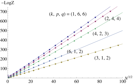
Figure 2: The free energy $(-\log{Z})$ is plotted against $N^{3/2}$ for some $(k,p,q)$. The straight lines show the perturbative free energy $(-\log{Z_{\text{pert}}})$.

2.8 A comment on the gravity dual

The $(p,q)$-model is expected to be the effective theory of $N$ M2-branes on the orbifold ($\mathbb{C}^{4}/(\mathbb{Z}_{p}\times\mathbb{Z}_{q}))/\mathbb{Z}_{k}$ Imamura:2008nn :

$$\phi_{A}:(z_{1},z_{2},z_{3},z_{4})\sim(e^{\frac{2\pi i}{q}}z_{1},e^{-\frac{2\pi i}{q}}z_{2},z_{3},z_{4}),$$

$$\phi_{B}:(z_{1},z_{2},z_{3},z_{4})\sim(z_{1},z_{2},e^{\frac{2\pi i}{p}}z_{3},e^{-\frac{2\pi i}{p}}z_{4}),$$

$$\phi_{C}:(z_{1},z_{2},z_{3},z_{4})\sim(e^{\frac{2\pi i}{kq}}z_{1},e^{-\frac{2\pi i}{kq}}z_{2},e^{\frac{2\pi i}{kp}}z_{3},e^{-\frac{2\pi i}{kp}}z_{4}).$$ (2.90)

This implies that the $(p,q)$-model is dual to M-theory on $AdS_{4}\times(S^{7}/(\mathbb{Z}_{p}\times\mathbb{Z}_{q}))/\mathbb{Z}_{k}$ with the metric

$$ds^{2}=\frac{R^{2}}{4}ds_{AdS_{4}}^{2}+R^{2}ds^{2}_{(S^{7}/(\mathbb{Z}_{p}\times\mathbb{Z}_{q}))/\mathbb{Z}_{k}},$$ (2.91)

where

$$R=(32\pi^{2}kpqN)^{1/6}l_{p}.$$ (2.92)

Since this background has many nontrivial 3-cycles, we could have discrete holonomies of the 3-form potential along the cycles as in the ABJ theory ABJ . For Imamura-Kimura type theory with equal ranks of gauge groups (without fractional branes), the discrete holonomies depend on the ordering of 5-branes in its type IIB brane construction. This has been studied in detail in Imamura:2009ur by analyzing monopole operators in general Imamura-Kimura type theory. According to the formula in Imamura:2009ur , we expect that the gravity dual of the $(p,q)$-model does not have the discrete holonomies.

There are some predictions on the free energy $-\log{Z}$ from the gravity side. First the free energy of the classical SUGRA with the boundary $S^{3}$ is given by (see e.g. Marino:2011nm )

$$F_{\rm SUGRA}=\frac{\pi\sqrt{2kpq}}{3}N^{3/2}.$$ (2.93)

Also by one-loop analysis of the 11d SUGRA on $AdS_{4}\times X_{7}$ with the smooth 7d manifold $X_{7}$, it is known that the one-loop free energy contains the following universal log-correction Bhattacharyya:2012ye

$$\frac{1}{4}\log{N}.$$ (2.94)

On the CFT side, this behavior comes from the the Airy functional behavior (2.89) in the perturbative free energy.

Next we give some comments on nonperturbative effects. Let us first recall the ABJM case. For the ABJM case ($p=q=1$), if we identify the M-theory circle with the orbifolding direction by $\mathbb{Z}_{k}$ and shrink the circle, then the 11d supergravity on $AdS_{4}\times S^{7}/\mathbb{Z}_{k}$ becomes the type IIA supergravity on $AdS_{4}\times\mathbb{CP}^{3}$. In the type II superstring on $AdS_{4}\times\mathbb{CP}^{3}$, we have worldsheet instanton effect, which comes from fundamental string wrapping the nontrivial 2-cycle $\mathbb{CP}^{1}$ in $\mathbb{CP}^{3}$ Cagnazzo:2009zh . From the M-theory viewpoint, this corresponds to an M2-brane wrapping the non-trivial 3-cycle $S^{3}/\mathbb{Z}_{k}$ in $S^{7}/\mathbb{Z}_{k}$. For the general $(p,q)$ case, we also expect that there are similar non-perturbative effects as in the ABJM case. Note that the orbifold (2.90) includes the nontrivial 3-cycle $(S^{3}/(\mathbb{Z}_{p}\times\mathbb{Z}_{q})/\mathbb{Z}_{k})$, which is obtained by taking $z_{2}=z_{4}=0$, for example. This implies the presence of non-perturbative effect coming from M2-brane wrapping this cycle, whose weight is given by

$$\exp{\Biggl{[}-T_{\rm M2}{\rm Vol}\left((S^{3}/(\mathbb{Z}_{p}\times\mathbb{Z}_{q}))/\mathbb{Z}_{k}\right)\Biggr{]}}=\exp{\Biggl{[}-\frac{R^{3}}{2kpq}\Biggr{]}}=\exp{\Biggl{[}-2\pi\sqrt{\frac{2N}{kpq}}\Biggr{]}}.$$ (2.95)

Since the 3-cycle becomes two-dimensional in the large-$k$ limit, we expect that this effect corresponds to the worldsheet instanton effect described by the fundamental string wrapping a 2-cycle in the type IIA superstring theory. One can see that the weight (2.95) of the worldsheet instanton effect computed from the gravity side correctly reproduces the weight (2.69) obtained by the matrix model, after changing the variable from the canonical to the grand canonical ensemble. This is also consistent with the planar solution of the $(1,q)$ model computed in appendix D.

3 Results on the $(1,q)$-model

In this section, we summarize some explicit results in the case of $p=1$. In this case, the system can be thought of as a one-parameter deformation of the ABJM Fermi-gas by $q$, or the deformation of the $N_{f}$ matrix model MePu ; GM by $k$. Therefore, the results for $k=1$ (and $q=N_{f}$) must reproduce those in the $N_{f}$ matrix model. Similarly, in the limit $q\to 1$ (with general $k$), the results must also reproduce those in the ABJM Fermi-gas.

3.1 Membrane instanton corrections

Let us first consider the membrane instanton corrections. First of all, one notices that the classical membrane instanton corrections $\mathcal{J}^{(0)}_{\text{M2,I}}$ and $\mathcal{J}^{(0)}_{\text{M2,III}}$ in (2.28) are divergent in the limit $p\to 1$. As was shown in MN2 , these divergences are, however, canceled by each other. One finds that after the cancellation, the finite part is given by

$$\widehat{\mathcal{J}}^{(0)}_{\text{M2,I}}(\mu)=\lim_{p\to 1}(\mathcal{J}^{(0)}_{\text{M2,I}}+\mathcal{J}^{(0)}_{\text{M2,III}})=\sum_{n=1}^{\infty}(\gamma^{(0)}_{n}(q)\mu+\delta^{(0)}_{n}(q))e^{-2n\mu},$$ (3.1)

where

$$\gamma_{n}^{(0)}(q) =-\frac{1}{2\pi^{2}n}\binom{2n}{n}\frac{\Gamma^{2}(-nq)}{\Gamma(-2nq)},$$ (3.2)

$$\delta_{n}^{(0)}(q) =-\frac{1}{4\pi^{2}n^{2}}\binom{2n}{n}\frac{\Gamma^{2}(-nq)}{\Gamma(-2nq)}\bigl{[}1+2n(H_{n}-H_{2n})+2nq\bigl{(}\psi(-nq)-\psi(-2nq)\bigr{)}\bigr{]}.$$

Here $H_{n}$ is the $n$-th harmonic number, and $\psi(z)=\partial_{z}\log\Gamma(z)$ is the digamma function. There is no limit problem for $\mathcal{J}^{(0)}_{\text{M2,II}}$:

$$\widehat{\mathcal{J}}^{(0)}_{\text{M2,II}}(\mu) =\lim_{p\to 1}\mathcal{J}^{(0)}_{\text{M2,II}}=\sum_{n=1}^{\infty}\alpha_{n}^{(0)}(q)e^{-\frac{2n\mu}{q}},$$ (3.3)

$$\alpha_{n}^{(0)}(q) =\frac{1}{2\pi n}\binom{2n}{n}\csc\left(\frac{2\pi n}{q}\right)\frac{\Gamma^{2}(-\frac{n}{q})}{\Gamma(-\frac{2n}{q})}.$$

Therefore, in the case of $p=1$, the large $\mu$ expansion (2.38) reduces to

$$\mathcal{J}_{\text{WKB}}^{p=1}(\mu,k)=\frac{C_{1,q}(k)}{3}\mu^{3}+B_{1,q}(k)\mu+A_{1,q}(k)+\widehat{\mathcal{J}}_{\text{M2,I}}(\mu,k)+\widehat{\mathcal{J}}_{\text{M2,II}}(\mu,k),$$ (3.4)

where

$$\widehat{\mathcal{J}}_{\text{M2,I}}(\mu,k) =\sum_{n=1}^{\infty}(\gamma_{n}(q,k)\mu+\delta_{n}(q,k))e^{-2n\mu},$$ (3.5)

$$\widehat{\mathcal{J}}_{\text{M2,II}}(\mu,k) =\sum_{n=1}^{\infty}\alpha_{n}(q,k)e^{-\frac{2n\mu}{q}}.$$

Note that $\alpha_{n}(q,k)=\alpha_{n}(q,1,k)$, not $\alpha_{n}(1,q,k)$. Acting the differential operator $\mathcal{D}^{(n)}$ in appendix B on the classical grand potential, one can find the WKB expansion of each coefficient.

Coefficients of $e^{-2n\mu}$.

To find the WKB expansions of $\gamma_{n}(q,k)$ and $\delta_{n}(q,k)$, we need to compute

$$\mathcal{D}^{(n)}(\mu e^{-2n\mu})\quad\text{and}\quad\mathcal{D}^{(n)}(e^{-2n\mu}).$$ (3.6)

The computation of $\gamma_{n}(q,k)$ is relatively easy, compared to the other instanton coefficients $\alpha_{n}(q,k),\delta_{n}(q,k)$. It takes the form

$$\gamma_{n}(q,k)=\frac{\gamma_{n}^{(0)}(q)}{k}D(-2n,1,q,k),$$ (3.7)

where, as mentioned in the previous section, $D(-2n,1,q,k)$ is obtained by replacing $\partial_{\mu}$ in the differential operator $\mathcal{D}$ by $-2n$. Therefore its WKB expansion is

$$D(-2n,1,q,k) =1-\frac{n^{2}(1+2n)q^{2}}{24(-1+2nq)}(\pi k)^{2}$$ (3.8)

$$\quad+\frac{n^{3}(1+2n)q^{3}\left(4-24n+4q-3nq+14n^{2}q\right)}{5760(-3+2nq)(-1+2nq)}(\pi k)^{4}+\mathcal{O}(k^{6}).$$

Since we have fixed $\mathcal{D}^{(n)}$ up to $n=17$, we can compute the WKB expansion up to $\mathcal{O}(k^{34})$. All of the following results reproduce the correct WKB expansions up to this order. From the WKB data, we find analytic expressions for $n=1,2$:

$$D(-2,1,q,k) ={}_{2}F_{1}\left(-\frac{q}{2},-\frac{q}{2};\frac{1}{2}-q;\sin^{2}\frac{\pi k}{2}\right),$$ (3.9)

$$D(-4,1,q,k) =\frac{1}{3}\,{}_{2}F_{1}\left(-q,-q;\frac{1}{2}-2q;\sin^{2}\frac{\pi k}{2}\right)+\frac{2}{3}\,{}_{2}F_{1}\left(-q,-2q;\frac{1}{2}-2q;\sin^{2}\frac{\pi k}{2}\right).$$

One can check that, in the limit $k\to 1$, $\gamma_{1}(q,k)$ and $\gamma_{2}(q,k)$ given by (3.7) with (3.9) reduce to

$$\gamma_{1}(q,1)=-\frac{1}{2\pi^{2}}\frac{\Gamma^{2}(-q/2)}{\Gamma(-q)},\qquad\gamma_{2}(q,1)=-\frac{1}{4\pi^{2}}\left(1+\frac{2}{\cos\pi q}\right)\frac{\Gamma^{2}(-q)}{\Gamma(-2q)},$$ (3.10)

which are in perfect agreement with the known results of $N_{f}$-matrix model in HO .

The constant part $\delta_{n}(q,k)$ is more involved. Both of (3.6) contribute to $\delta_{n}(q,k)$. The latter contribution is just $D(-2n,1,q,k)$. A simple computation shows that the $\mu$-independent contribution of the former is given by $\partial_{s}D(s,1,q,k)|_{s=-2n}$. We conclude that

$$\delta_{n}(q,k)=\frac{\delta_{n}^{(0)}(q)}{k}\Bigl{(}D(-2n,1,q,k)+\partial_{s}D(s,1,q,k)|_{s=-2n}\Bigr{)},$$ (3.11)

where the WKB expansion of $\partial_{s}D(s,1,q,k)|_{s=-2n}$ is given by

$$\partial_{s}D(s,1,q,k)|_{s=-2n}=\frac{nq^{2}\left(-1-3n+nq+4n^{2}q\right)}{24(-1+2nq)^{2}}(\pi k)^{2}$$ (3.12)

$$\qquad-\frac{n^{2}q^{3}}{2880(-3+2nq)^{2}(-1+2nq)^{2}}\bigl{[}-3(-3+16n+60n^{2})+(9-n+126n^{2}$$

$$\qquad\quad+510n^{3})q-2n(8+13n+48n^{2}+212n^{3})q^{2}+2n^{2}(2+5n$$

$$\qquad\quad+12n^{2}+56n^{3})q^{3}\bigr{]}(\pi k)^{4}+\mathcal{O}(k^{6}).$$

It is difficult to guess an exact form of this expansion even for $n=1$.

Coefficients of $e^{-2n\mu/q}$.

Next, let us consider the second type correction $\widehat{\mathcal{J}}_{\text{M2,II}}$. The coefficient $\alpha_{n}(q,k)$ is given by

$$\alpha_{n}(q,k)=\frac{\alpha_{n}^{(0)}(q)}{k}D\left(-\frac{2n}{q},1,q,k\right).$$ (3.13)

The WKB expansion of $D(-2n/q,1,q,k)$ is given by

$$D\left(-\frac{2n}{q},1,q,k\right) =1-\frac{n^{2}(2n+q)}{24q(-1+2n)}(\pi k)^{2}$$ (3.14)

$$\quad+\frac{n^{3}(2n+q)\left(-24n+14n^{2}+4q-3nq+4q^{2}\right)}{5760q^{2}(-3+2n)(-1+2n)}(\pi k)^{4}+\mathcal{O}(k^{6}).$$

It is not easy to find out an exact expression of this expansion, but for $n=1$ we find a surprisingly simple expression in terms of the $q$-gamma function,

$$D\left(-\frac{2}{q},1,q,k\right)=\frac{\Gamma^{2}(1+1/q)}{\Gamma(1+2/q)}\frac{\Gamma_{\mathfrak{q}}(1+2/q)}{\Gamma_{\mathfrak{q}}^{2}(1+1/q)}\mathfrak{q}^{-\frac{1}{2q^{2}}},\quad\mathfrak{q}=e^{\pi ikq},$$ (3.15)

where $\Gamma_{\mathfrak{q}}(z)$ is the $q$-gamma function defined in appendix E. As we will see in the next section, this conjecture comes from the analysis of this instanton coefficient for the $1/q\in\mathbb{Z}$ case (4.21). When $kq\in\mathbb{R}$, there is a subtlety of the definition of the $q$-gamma function due to $|\mathfrak{q}|=1$. As explained in appendix E, one can define the $q$-gamma function with $|\mathfrak{q}|=1$ by regularizing the infinite product using the zeta-function regulariation. Using the result (E.12) in appendix E, one obtains the all-order WKB expansion

$$D\left(-\frac{2}{q},1,q,k\right)=\exp\left[\sum_{n=1}^{\infty}\frac{(-1)^{n-1}B_{2n}}{2n(2n+1)!}\left(2B_{2n+1}\left(1+q^{-1}\right)-B_{2n+1}\left(1+2q^{-1}\right)\right)(\pi kq)^{2n}\right]$$ (3.16)

$$\qquad=\frac{\pi k}{2}\cot\left(\frac{\pi k}{2}\right)\exp\left[\sum_{n=1}^{\infty}\frac{(-1)^{n-1}B_{2n}}{2n(2n+1)!}\left(2B_{2n+1}\left(q^{-1}\right)-B_{2n+1}\left(2q^{-1}\right)\right)(\pi kq)^{2n}\right],$$

where $B_{n}$ and $B_{n}(x)$ are the Bernoulli number and the Bernoulli polynomial, respectively. From the first line to the second line in (3.16), we have used the identity

$$B_{m}(1+w)=B_{m}(w)+mw^{m-1}.$$ (3.17)

By using an integral representation of the Bernoulli polynomial Bernoulli

$$B_{2n+1}(w)=(-1)^{n-1}(2n+1)\int_{0}^{\infty}dt\,\frac{\sin 2\pi w}{\cosh 2\pi t-\cos 2\pi w}t^{2n},\qquad 0\leq w\leq 1,$$ (3.18)

one can perform the resummation of (3.16). For $q\geq 2$, one easily finds

$$D\left(-\frac{2}{q},1,q,k\right)=\frac{\pi k}{2}\cot\left(\frac{\pi k}{2}\right)\exp[I_{1}(q,k)],\qquad q\geq 2,$$ (3.19)

where

$$I_{1}(q,k)=\int_{0}^{\infty}dt\frac{4\sin^{2}\frac{\pi}{q}\sin\frac{2\pi}{q}(\cosh 2\pi t+2\cos^{2}\frac{\pi}{q})}{(\cosh 2\pi t-\cos\frac{2\pi}{q})(\cosh 2\pi t-\cos\frac{4\pi}{q})}\log\left(\frac{\sinh(\pi kqt/2)}{\pi kqt/2}\right).$$ (3.20)

For $1\leq q\leq 2$, to use the integral representation (3.18), we further need to shift the argument by using (3.17) with $w=2q^{-1}-1$. Then we find

$$D\left(-\frac{2}{q},1,q,k\right)=\frac{\pi k}{2}\cot\left(\frac{\pi k}{2}\right)\frac{\sin\frac{\pi k}{2}(2-q)}{\frac{\pi k}{2}(2-q)}\exp[I_{1}(q,k)],\qquad 1\leq q\leq 2,$$ (3.21)

where $I_{1}(q,k)$ is the same as above. In a similar way, one also obtains the integral representation for $0<q<1$. These integral representations are very useful to understand the pole structure of $\alpha_{1}(q,k)$. Since the integrand of $I_{1}(q,k)$ is exponentially dumped for large $t$ and does not have singularities in the integral domain for $q\neq 1,2$ and finite $k$, $I_{1}(q,k)$ takes in a finite real value and hence does not have any singularities for $k>0$. Thus the singularities of $\alpha_{1}(q,k)$ come only from the cotangent factor in (3.19) or (3.21). In figure 3, we illustrate these for $q=3$.

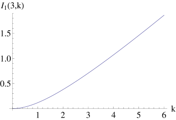
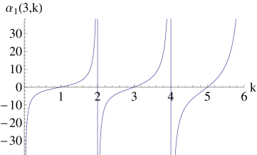
Figure 3: We plot $I_{1}(3,k)$ (Left) and $\alpha_{1}(3,k)$ (Right) as functions of $k$. In general, $\alpha_{1}(q,k)$ has simple poles at even $k$.

3.2 Worldsheet instanton corrections

In the case of $p=1$, the worldsheet instanton corrections take the form

$$\left.\mathcal{J}_{\text{WS}}(\mu,k)\right|_{p=1}=\sum_{m=1}^{\infty}d_{m}(1,q,k)e^{-\frac{4m}{qk}\mu}.$$ (3.22)

From a consistency with the results for various integral $(q,k)$ (see appendix F), we conjecture the exact form of worldsheet instanton coefficients for $m=1,2$:

$$d_{1}(1,q,k) =\frac{q}{\sin\frac{2\pi}{k}\sin\frac{2\pi}{qk}},$$ (3.23)

$$d_{2}(1,q,k) =-\frac{1}{2\sin^{2}\frac{2\pi}{qk}}-\frac{q^{2}}{\sin^{2}\frac{2\pi}{k}}+\frac{q\sin\frac{6\pi}{qk}}{2\sin\frac{4\pi}{k}\sin\frac{2\pi}{qk}\sin\frac{4\pi}{qk}}.$$

Note that these are also consistent with the planar free energy computed in appendix D. In the limit $q\to 1$, these precisely reproduce the worldsheet instanton corrections in the ABJM Fermi-gas computed in HMO2 . Also, for $q=2$, (3.23) reproduces the worldsheet instanton coefficients of $(p,q)=(1,2)$ model found in MN2 .

3.3 Pole cancellations

Since we have determined some of the instanton coefficients analytically, we can see the pole cancellations in some special limits of $(q,k)$ beyond the semi-classical approximation. These are important non-trivial tests of our conjectures.

ABJM limit.

In the limit $q\to 1$, all of $\alpha_{n}(q,k)$, $\gamma_{n}(q,k)$ and $\delta_{n}(q,k)$ are divergent. Let us see the cancellation of these divergences for $n=1$. We first notice that $I_{1}(q,k)$ behaves as

$$\lim_{q\to 1}I_{1}(q,k)=\mathcal{O}((q-1)^{3}).$$ (3.24)

Using the integral representation (3.21), one finds that the divergence of $\alpha_{1}(q,k)$ is given by

$$\lim_{q\to 1^{+}}\alpha_{1}(q,k)e^{-\frac{2\mu}{q}}=-\frac{4}{\pi^{2}k}\cos\left(\frac{\pi k}{2}\right)\biggl{[}\frac{1}{2(q-1)^{2}}+\left(\mu+1-\frac{\pi k}{4}\cot\frac{\pi k}{2}\right)\frac{1}{q-1}$$ (3.25)

$$+\mu^{2}+\left(1-\frac{\pi k}{2}\cot\frac{\pi k}{2}\right)\mu+\frac{1}{2}+\frac{\pi^{2}(4-k^{2})}{16}-\frac{\pi k}{2}\cot\frac{\pi k}{2}+\mathcal{O}(q-1)\biggr{]}e^{-2\mu}.$$

The divergence of $\gamma_{1}(q,k)$ is

$$\lim_{q\to 1}\gamma_{1}(q,k)=\frac{4}{\pi^{2}k}\cos\left(\frac{\pi k}{2}\right)\left[\frac{1}{q-1}+1+\mathcal{O}(q-1)\right].$$ (3.26)

Thus we get

$$\lim_{q\to 1^{+}}\left(\alpha_{1}(q,k)e^{-\frac{2\mu}{q}}+\mu\gamma_{1}(q,k)e^{-2\mu}\right)$$ (3.27)

$$\quad=-\frac{4}{\pi^{2}k}\cos\left(\frac{\pi k}{2}\right)\biggl{[}\frac{1}{2(q-1)^{2}}+\left(1-\frac{\pi k}{4}\cot\frac{\pi k}{2}\right)\frac{1}{q-1}\biggr{]}e^{-2\mu}$$

$$\quad\quad+(a_{1}(k)\mu^{2}+b_{1}(k)\mu+c_{1}(k)+\delta c_{1}(k))e^{-2\mu}+\mathcal{O}(q-1),$$

where

$$a_{1}(k) =-\frac{4}{\pi^{2}k}\cos\frac{\pi k}{2},\qquad\quad b_{1}(k)=\frac{2}{\pi}\cos\frac{\pi k}{2}\cot\frac{\pi k}{2},$$ (3.28)

$$c_{1}(k) =\left(-\frac{2}{3k}+\frac{5k}{12}+\frac{1}{\pi}\cot\frac{\pi k}{2}+\frac{k}{2}\csc^{2}\frac{\pi k}{2}\right)\cos\frac{\pi k}{2},$$

and

$$\delta c_{1}(k)=-\frac{4}{\pi^{2}k}\cos\left(\frac{\pi k}{2}\right)\left(\frac{1}{2}+\frac{\pi^{2}(4-k^{2})}{16}-\frac{\pi k}{2}\cot\frac{\pi k}{2}\right)-c_{1}(k).$$ (3.29)

The divergence of the $\mu$-dependent part is precisely canceled. Furthermore, the coefficients $a_{1}(k)$ and $b_{1}(k)$ in the finite part perfectly agree with the results in the ABJM Fermi-gas HMO2 . The divergence of the $\mu$-independent part must be canceled by $\delta_{1}(q,k)$. This means that $\delta_{1}(q,k)$ must behave as

$$\lim_{q\to 1^{+}}\delta_{1}(q,k)=\frac{4}{\pi^{2}k}\cos\left(\frac{\pi k}{2}\right)\biggl{[}\frac{1}{2(q-1)^{2}}+\left(1-\frac{\pi k}{4}\cot\frac{\pi k}{2}\right)\frac{1}{q-1}\biggr{]}-\delta c_{1}(k).$$ (3.30)

This is regarded as the constraint for $\delta_{1}(q,k)$.

$k\rightarrow 2$ limit.

Let us consider another limit $k\to 2$. In this limit, the coefficient $\alpha_{1}(q,k)$ of $e^{-\frac{2\mu}{q}}$ diverges, as shown in figure 3. This divergence must be canceled by the leading worldsheet instanton correction of order $e^{-\frac{4\mu}{qk}}$. It is easy to find

$$\lim_{k\to 2}d_{1}(1,q,k)e^{-\frac{4\mu}{qk}}=\biggl{[}\frac{2q}{\pi\sin\frac{\pi}{q}}\frac{1}{k-2}+\frac{2\mu+q+\pi\cot\frac{\pi}{q}}{\pi\sin\frac{\pi}{q}}+\mathcal{O}(k-2)\biggr{]}e^{-\frac{2\pi}{q}}.$$ (3.31)

Using the integral expression (3.19) or (3.21), we also find

$$\lim_{k\to 2}\alpha_{1}(q,k)e^{-\frac{2\mu}{q}}=\biggl{[}-\frac{2q}{\pi\sin\frac{\pi}{q}}\frac{1}{k-2}-\frac{\cot\frac{\pi}{q}}{\sin\frac{\pi}{q}}+\mathcal{O}(k-2)\biggr{]}e^{-\frac{2\pi}{q}}.$$ (3.32)

The singular parts are indeed canceled as expected. The finite part is finally given by

$$\lim_{k\to 2}\left(\alpha_{1}(q,k)e^{-\frac{2\mu}{q}}+d_{1}(1,q,k)e^{-\frac{4\mu}{qk}}\right)=\frac{2\mu+q}{\pi\sin\frac{\pi}{q}}e^{-\frac{2\pi}{q}}.$$ (3.33)

This correctly reproduces the coefficient (F.13) of $e^{-2\mu/q}$ for the $(p,q,k)=(1,q,2)$ case (see appendix F).

$k\rightarrow 2n$ limit.

More generally, $\alpha_{1}(q,k)$ has a pole at $k=2n$ (even integer). From the integral expression (3.19), we find that $\alpha_{1}(q,k)$ behaves in the limit $k\to 2n$ as

$$\lim_{k\to 2n}\alpha_{1}(q,k)=-\frac{1}{k-2n}\frac{2q}{\pi\sin\frac{2\pi}{q}}\prod_{j=1}^{n}\frac{\sin\frac{\pi(n+j)}{nq}}{\sin\frac{\pi j}{nq}}+\mathcal{O}(1).$$ (3.34)

This pole should be canceled by the worldsheet $n$-instanton

$$\lim_{k\to 2n}\left(\alpha_{1}(q,k)e^{-\frac{2\mu}{q}}+d_{n}(1,q,k)e^{-\frac{4n\mu}{qk}}\right)=\text{finite}.$$ (3.35)

One can see that $d_{2}(1,q,k)$ in (3.23) indeed has the correct pole structure at $k=4$ satisfying the condition (3.35). For $n\geq 3$, this pole cancellation condition (3.35) gives the constraint for a possible form of $d_{n}(1,q,k)$.

4 Results on the $(p,q)$-model

In this section, we give explicit results for the general $(p,q)$-model. The basic strategy is the same as in the case of $p=1$. We compute the WKB expansion of each membrane instanton coefficient, and then conjecture its analytic form. Since the WKB expansions become much more complicated than those for the $(1,q)$-model, it is harder to determine their analytic forms. To fix the worldsheet instanton corrections, we use the exact results for various integral $(p,q,k)$ in appendix F.

4.1 Exact partition function for $N=2$

We first compute the spectral zeta function at $s=2$, exactly. It is easy to find that $\zeta_{\rho}(1)$ is exactly given by

$$\zeta_{\rho}(1)=\int_{-\infty}^{\infty}dx\,\rho(x,x)=\frac{1}{4\pi^{2}k}\frac{\Gamma^{2}(\frac{p}{2})\Gamma^{2}(\frac{q}{2})}{\Gamma(p)\Gamma(q)}.$$ (4.1)

Also, $\zeta_{\rho}(2)$ can be computed as follows,

$$\zeta_{\rho}(2) =\int dx\left\langle x\right|\frac{1}{(2\cosh\frac{\hat{P}}{2})^{p}}\frac{1}{(2\cosh\frac{\hat{Q}}{2})^{q}}\frac{1}{(2\cosh\frac{\hat{P}}{2})^{p}}\frac{1}{(2\cosh\frac{\hat{Q}}{2})^{q}}\left|x\right\rangle$$ (4.2)

$$=\int dxdy\left\langle x\right|\frac{1}{(2\cosh\frac{\hat{P}}{2})^{p}}\left|y\right\rangle\left\langle y\right|\frac{1}{(2\cosh\frac{\hat{P}}{2})^{p}}\left|x\right\rangle\frac{1}{(2\cosh\frac{x}{2})^{q}}\frac{1}{(2\cosh\frac{y}{2})^{q}}.$$

By using the fact that $\left\langle x\right|G(\hat{P})\left|y\right\rangle$ depends only on $x-y$ and shifting the integral variable $x\to x+y$, we find

$$\zeta_{\rho}(2) =\int\frac{dxdy}{(2\pi k)^{2}}\Big{|}\left\langle x-y\right|\frac{1}{(2\cosh\frac{\hat{P}}{2})^{p}}\left|0\right\rangle\Big{|}^{2}\frac{1}{(2\cosh\frac{x}{2})^{q}}\frac{1}{(2\cosh\frac{y}{2})^{q}}$$ (4.3)

$$=\int\frac{dx}{2\pi k}\Big{|}\left\langle x\right|\frac{1}{(2\cosh\frac{\hat{P}}{2})^{p}}\left|0\right\rangle\Big{|}^{2}{\cal F}(q,x),$$

where

$${\cal F}(q,x)=\int_{-\infty}^{\infty}\frac{dy}{2\pi k}\frac{1}{(2\cosh\frac{x+y}{2})^{q}}\frac{1}{(2\cosh\frac{y}{2})^{q}}=\frac{1}{2\pi k}\frac{\Gamma(q)^{2}}{\Gamma(2q)}~{}{}_{2}F_{1}\left(\frac{q}{2},\frac{q}{2};\frac{1}{2}+q;-\sinh^{2}\frac{x}{2}\right).$$ (4.4)

Using the Fourier transform

$$\left\langle x\right|\frac{1}{(2\cosh\frac{\hat{P}}{2})^{p}}\left|0\right\rangle=\frac{1}{2\pi}\operatorname{B}\Big{(}\frac{p}{2}+\frac{ix}{2\pi k},\frac{p}{2}-\frac{ix}{2\pi k}\Big{)},$$ (4.5)

we finally find

$$\zeta_{\rho}(2)=\frac{\operatorname{B}(q,q)}{8\pi^{3}k}\int_{-\infty}^{\infty}dx\,\operatorname{B}^{2}\Big{(}\frac{p}{2}+ix,\frac{p}{2}-ix\Big{)}\,{}_{2}F_{1}\left(\frac{q}{2},\frac{q}{2};\frac{1}{2}+q;-\sinh^{2}\pi kx\right),$$ (4.6)

where we have rescaled the integration variable $x\to 2\pi kx$. Note that this is an exact expression. Recalling the relation (2.15), the exact partition functions for $N=1,2$ are given by

$$Z(1,k)=\zeta_{\rho}(1),\qquad Z(2,k)=-\frac{1}{2}\zeta_{\rho}(2)+\frac{1}{2}\zeta_{\rho}(1)^{2}.$$ (4.7)

In the case of $p=q=1$, $Z(2,k)$ correctly reduces to the exact partition function for $N=2$ in the ABJM theory, computed in Okuyama .

For the spectral trace $\zeta_{\rho}(\ell)$ with general $\ell\in\mathbb{Z}_{>0}$, we conjecture that it has a simple integral representation

$$\zeta_{\rho}(\ell)=\int\frac{dPdQ}{2\pi\hbar}V(Q)U(P)e^{(-1)^{\ell}i\hbar\partial_{Q}\partial_{P}}V(Q)U(P)e^{(-1)^{\ell-1}i\hbar\partial_{Q}\partial_{P}}V(Q)U(P)\cdots e^{i\hbar\partial_{Q}\partial_{P}}V(Q)U(P).$$ (4.8)

Here, for simplicity, we have introduced the notation $V(Q)=(2\cosh\frac{Q}{2})^{-q},U(P)=(2\cosh\frac{P}{2})^{-p}$, and the derivatives in (4.8) act on all functions on their right. One can show that, for $\ell=2$, (4.8) indeed agrees with (4.6). Although we do not have a proof of (4.8) for $\ell\geq 3$, we have checked that this conjectured expression (4.8) correctly reproduces the WKB expansion.

4.2 Membrane instanton corrections

In this subsection, we consider the membrane instanton corrections.

Coefficients of $e^{-n\mu}$.

Let us first consider the coefficient of $e^{-n\mu}$ in (2.43). The WKB expansion of $D(-n,p,q,k)$ up to $\mathcal{O}(k^{4})$ is given by

$$D(-n,p,q,k)=1-\frac{n^{2}(n^{2}-1)p^{2}q^{2}}{96(-1+np)(-1+nq)}(\pi k)^{2}$$ (4.9)

$$\quad+\frac{n^{3}(n^{2}-1)p^{3}q^{3}\left(80n-24p-24n^{2}p-24q-24n^{2}q+17npq+7n^{3}pq\right)}{92160(-3+np)(-1+np)(-3+nq)(-1+nq)}(\pi k)^{4}+\mathcal{O}(k^{6}).$$

One notices that $D(-1,p,q,k)$ does not receive the quantum corrections: $D(-1,p,q,k)=1$. This is indeed the case. Since $\zeta_{\rho}(1)$ does not receive any corrections, we have $D(1,p,q,k)=1$ for any $(p,q)$. Using the reflection symmetry (2.49), we conclude that $D(-1,p,q,k)=1$. Therefore $\beta_{1}(p,q,k)$ is exactly given by

$$\beta_{1}(p,q,k)=\frac{\beta_{1}^{(0)}(p,q)}{k}=\frac{1}{4\pi^{2}k}\frac{\Gamma^{2}(-\frac{p}{2})}{\Gamma(-p)}\frac{\Gamma^{2}(-\frac{q}{2})}{\Gamma(-q)}.$$ (4.10)

Moreover, the WKB expansion for $n=2$ has the following remarkable structure:

$$D(-2,p,q,k)=\sum_{n=0}^{\infty}\frac{(-1)^{n}}{(2n)!}f_{n}(p)f_{n}(q)\left(\frac{\pi k}{2}\right)^{2n},$$ (4.11)

where a generating function of $f_{n}(p)$ is given by

$$\sum_{n=0}^{\infty}\frac{f_{n}(p)}{(2n)!}z^{2n}={}_{2}F_{1}\left(-\frac{p}{2},-\frac{p}{2};\frac{1}{2}-p;\sin^{2}z\right).$$ (4.12)

More explicitly, $f_{n}(p)$ is given by

$$f_{n}(p)=\sum_{m=0}^{n}\frac{(-1)^{n}}{2^{2m-1}m!}\frac{(-\frac{p}{2})_{m}^{2}}{(\frac{1}{2}-p)_{m}}\sum_{j=1}^{m}(-1)^{j}\binom{2m}{m-j}(2j)^{2n}.$$ (4.13)

In the previous subsection, we have already computed $\zeta_{\rho}(2)$. From (4.6), one finds that

$$D(2,p,q,k)=\frac{\Gamma(2p)}{2\pi\Gamma^{2}(p)}\int_{-\infty}^{\infty}dx\,\operatorname{B}^{2}\Big{(}\frac{p}{2}+ix,\frac{p}{2}-ix\Big{)}\,{}_{2}F_{1}\left(\frac{q}{2},\frac{q}{2};\frac{1}{2}+q;-\sinh^{2}\pi kx\right).$$ (4.14)

Using the symmetry (2.49), one immediately obtains

$$D(-2,p,q,k)=D(2,-p,-q,k)$$ (4.15)

$$=\frac{\Gamma(-2p)}{2\pi\Gamma^{2}(-p)}\int_{-\infty}^{\infty}dx\,\operatorname{B}^{2}\Big{(}-\frac{p}{2}+ix,-\frac{p}{2}-ix\Big{)}\,{}_{2}F_{1}\left(-\frac{q}{2},-\frac{q}{2};\frac{1}{2}-q;-\sinh^{2}\pi kx\right).$$

One can understand the factorized structure (4.11) of $D(-2,p,q,k)$ from the expression of $\zeta_{\rho}(2)$ in (4.8). We emphasize that this expression is valid for any $(p,q)$. In particular, for $p=1,2,3,4$, we find the following analytic expressions

$$D(-2,1,q,k) ={}_{2}F_{1}\left(-\frac{q}{2},-\frac{q}{2},\frac{1}{2}-q;\sin^{2}\frac{\pi k}{2}\right),$$ (4.16)

$$D(-2,2,q,k) =\frac{2}{3}+\frac{1}{3}\,{}_{2}F_{1}\left(-\frac{q}{2},-\frac{q}{2},\frac{1}{2}-q;\sin^{2}\pi k\right),$$

$$D(-2,3,q,k) =\frac{9}{10}\,{}_{2}F_{1}\left(-\frac{q}{2},-\frac{q}{2},\frac{1}{2}-q;\sin^{2}\frac{\pi k}{2}\right)+\frac{1}{10}\,{}_{2}F_{1}\left(-\frac{q}{2},-\frac{q}{2},\frac{1}{2}-q;\sin^{2}\frac{3\pi k}{2}\right),$$

$$D(-2,4,q,k) =\frac{18}{35}+\frac{16}{35}\,{}_{2}F_{1}\left(-\frac{q}{2},-\frac{q}{2},\frac{1}{2}-q;\sin^{2}\pi k\right)+\frac{1}{35}\,{}_{2}F_{1}\left(-\frac{q}{2},-\frac{q}{2},\frac{1}{2}-q;\sin^{2}2\pi k\right).$$

Similarly, if either $D(n,p,q,k)$ or $D(-n,p,q,k)$ ($n\in\mathbb{Z}_{>0}$) is known, one can know the other by the symmetry (2.49) and the analytic continuation $(p,q)\to(-p,-q)$. By matching the WKB data, we find the analytic form of $D(-n,p,q,k)$ for some other cases

$$D(-3,2,q,k)= \frac{3}{5}\,_{2}F_{1}\left(-q,-\frac{q}{2};\frac{1}{2}-\frac{3q}{2};\sin^{2}\pi k\right)+\frac{2}{5},$$ (4.17)

$$D(-3,4,q,k)= \frac{8}{77}\,_{2}F_{1}\left(-\frac{3q}{2},-q;\frac{1}{2}-\frac{3q}{2};\sin^{2}\pi k\right)+\frac{48}{77}\,_{2}F_{1}\left(-q,-\frac{q}{2};\frac{1}{2}-\frac{3q}{2};\sin^{2}\pi k\right)$$

$$+\frac{3}{77}\,_{2}F_{1}\left(-q,-\frac{q}{2};\frac{1}{2}-\frac{3q}{2};\sin^{2}2\pi k\right)+\frac{18}{77},$$

$$D(-4,2,q,k)= \frac{16}{35}\,_{2}F_{1}\left(-3q,-q;\frac{1}{2}-2q;\sin^{2}\frac{\pi k}{2}\right)+\frac{2}{35}\,_{2}F_{1}\left(-2q,-q;\frac{1}{2}-2q;\sin^{2}\pi k\right)$$

$$+\frac{9}{35}\,_{2}F_{1}\left(-q,-q;\frac{1}{2}-2q;\sin^{2}\pi k\right)+\frac{8}{35}.$$

Note that when $q$ is an integer, the hypergeometric series in (4.16) and (4.17) are truncated to a finite sum, and they are reduced to some combinations of trignometric functions.

Coefficients of $e^{-2n\mu/p}$.

The WKB expansion of the coefficient of $e^{-2n\mu/p}$ up to $\mathcal{O}(k^{4})$ is

$$D\left(-\frac{2n}{p},p,q,k\right)=1-\frac{n^{2}q^{2}(2n-p)(2n+p)}{24p(-1+2n)(-p+2nq)}(\pi k)^{2}$$ (4.18)

$$\qquad\quad+\frac{n^{3}q^{3}(2n-p)(2n+p)}{5760p^{2}(-3+2n)(-1+2n)(-3p+2nq)(-p+2nq)}\bigl{(}80np-48n^{2}p$$

$$\qquad\qquad\qquad\qquad-12p^{3}-48n^{2}q+28n^{3}q-12p^{2}q+17np^{2}q\bigr{)}(\pi k)^{4}+\mathcal{O}(k^{6}).$$

Here we focus on the $n=1$ case, i.e., the coefficient of $e^{-2\mu/p}$. For the case of $q/p=m\in\mathbb{Z}_{>0}$, we find that the following expression correctly reproduces the WKB expansion up to $\mathcal{O}(k^{34})$

$$D\left(-\frac{2}{p},p,mp,k\right)=\frac{m!^{2}}{(2m)!}\sum_{\sum_{j}j\lambda_{j}=m}\prod_{j=1}^{m}\frac{1}{\lambda_{j}!}\left[\frac{(-1)^{j-1}}{j}\frac{mp\sin\pi jk}{\sin\frac{\pi jkp}{2}}\right]^{\lambda_{j}}.$$ (4.19)

One can easily show that this can be rewritten as a contour integral

$$D\left(-\frac{2}{p},p,mp,k\right)= \frac{\Gamma(m+1)^{2}}{\Gamma(2m+1)}\oint_{z=0}\frac{dz}{2\pi iz^{m+1}}\exp\left[mp\sum_{j=1}^{\infty}\frac{(-1)^{j-1}}{j}\frac{\sin\pi jk}{\sin\frac{\pi jkp}{2}}\right]$$

$$= \frac{\Gamma(m+1)^{2}}{\Gamma(2m+1)}\oint_{z=0}\frac{dz}{2\pi iz^{m+1}}\left[\prod_{n=0}^{\infty}\frac{1+z\mathfrak{q}^{n-\frac{1}{p}+\frac{1}{2}}}{1+z\mathfrak{q}^{n+\frac{1}{p}+\frac{1}{2}}}\right]^{mp},$$ (4.20)

where $\mathfrak{q}=e^{i\pi kp}$. In particular, when $(p,q)=(1/m,1)$, this integral can be evaluated explicitly by expanding the integrand using the $q$-binomial formula. By picking up the coefficient of $z^{m}$, we find

$$D\left(-2m,\frac{1}{m},1,k\right)=\frac{m!^{2}}{(2m)!}\frac{\prod_{j=1}^{2m}\sin\frac{\pi kj}{2m}}{\prod_{j=1}^{m}\sin^{2}\frac{\pi kj}{2m}}.$$ (4.21)

By noticing that (4.21) can be written as a combination of $q$-factorials, we have arrived at the conjecture in the previous section that the coefficient of $e^{-2\mu/p}$ is given by the $q$-gamma function (3.15) for the general $(p,1)$ case. Also, for the $(p,q)=(2/m,2)$ case, the integral (4.20) can be evaluated exactly thanks to the formula (3.9.1) in koekoek

$$D\left(-m,\frac{2}{m},2,k\right) =\frac{m!^{2}}{(2m)!}{}_{2}\phi_{1}(\mathfrak{q}^{-m},\mathfrak{q}^{-m},\mathfrak{q};\mathfrak{q},\mathfrak{q}^{m+1})$$

$$=\frac{m!^{2}}{(2m)!}\sum_{l=0}^{m}\frac{\prod_{j=1}^{m}\sin^{2}\frac{\pi kj}{m}}{\prod_{j=1}^{l}\sin^{2}\frac{\pi kj}{m}\prod_{j=1}^{m-l}\sin^{2}\frac{\pi kj}{m}},$$ (4.22)

where ${}_{2}\phi_{1}(\mathfrak{q}^{a},\mathfrak{q}^{a},\mathfrak{q}^{c};\mathfrak{q},z)$ denotes the basic $q$-hypergeometric series. This suggests that the the coefficient of $e^{-2\mu/p}$ for the general $(p,2)$ case is given by a certain analytic continuation of (4.22) to a non-integer $m$. However, compared to the $q$-gamma function appearing in the $(p,1)$ case, the precise definition of the $q$-hypergeometric series with $|\mathfrak{q}|=1$ is much more subtle (see nishizawa for some proposal). We leave it as an interesting future problem. For $q>2$, the integral (4.20) is hard to evaluate explicitly.

When $m=q/p$ is not integer, the contour integral representation (4.20) is no longer correct due to the branch cut of $1/z^{q/p+1}$. Instead, we conjecture that the coefficient of $e^{-2\mu/p}$ for the general $(p,q)$ case is given by the following integral along the real segment $0<z<1$

$$D\left(-\frac{2}{p},p,q,k\right)=1+\frac{2\Gamma(-2q/p)}{\Gamma^{2}(-q/p)}\int_{0}^{1}\frac{dz}{z^{1+q/p}}\biggl{(}e^{qF(p,k,z)}-(1+z)^{2q/p}\biggr{)},$$ (4.23)

with

$$F(p,k,z)=2\sum_{n=0}^{\infty}\frac{(-1)^{n-1}}{(2n+1)!}B_{2n+1}\left(\frac{1}{2}+\frac{1}{p}\right)\operatorname{Li}_{1-2n}(-z)(\pi kp)^{2n}.$$ (4.24)

Here $\operatorname{Li}_{n}(z)$ denotes the polylogarithm. We do not have a proof of this conjecture, but we have confirmed that it correctly reproduces the WKB expansion up to $\mathcal{O}(k^{34})$. For $p\geq 2$, one can rewrite $F(p,k,z)$ as the following integral form by using (3.18),

$$F(p,k,z)=\int_{0}^{\infty}dt\frac{\sin\frac{2\pi}{p}}{\cosh 2\pi t+\cos\frac{2\pi}{p}}\log(1+2z\cosh\pi kpt+z^{2}),\qquad p\geq 2.$$ (4.25)

For $p<2$, one has to shift the argument of the Bernoulli polynomial in (4.24) to use the integral representation.

4.3 Worldsheet instanton corrections

As in the same way in the previous section, we can compute the worldsheet instanton corrections for various integral $(p,q,k)$ (see appendix F). From these data, we conjecture that the leading worldsheet instanton correction in (2.70) is given by

$$d_{1}(p,q,k)=\frac{pq}{\sin\frac{2\pi}{pk}\sin\frac{2\pi}{qk}}.$$ (4.26)

To guess the higher order corrections is not easy. For the $(1,q)$-model, we conjectured the 2-instanton correction in (3.23). We also conjecture the 2-instanton correction for the $(2,q)$-model as

$$d_{2}(2,q,k)=-\frac{2}{\sin^{2}\frac{2\pi}{qk}}-\frac{q^{2}}{\sin^{2}\frac{\pi}{k}}+\frac{q(2+\cos\frac{4\pi}{qk})}{\sin\frac{2\pi}{k}\sin\frac{4\pi}{qk}}.$$ (4.27)

One can check that in the limit $q\to 2$ this reproduces the result of $(p,q)=(2,2)$ model in MN2 .

4.4 Pole cancellations

The worldsheet 1-instanton coefficient (4.26) for the general $(p,q)$ case has a pole at $k=2/q$

$$\lim_{k\to\frac{2}{q}}d_{1}(p,q,k)e^{-\frac{4\mu}{pqk}}=\frac{1}{\pi\sin\frac{\pi q}{p}}\left[\frac{2p}{k-\frac{2}{q}}+\pi q^{2}\cot\frac{\pi q}{p}+q(2\mu+p)\right]e^{-\frac{2\mu}{p}}.$$ (4.28)

This pole should be canceled by the membrane 1-instanton coefficient $\alpha_{1}(p,q,k)$ of $e^{-2\mu/p}$ given by (4.23). We have checked numerically that the membrane 1-instanton coefficient (4.23) has the correct pole and residue to cancel the pole of worldsheet instanton (4.28). Similarly, the pole of the membrane 1-instanton at $k=4/q$ should be canceled by the worldsheet 2-instanton

$$\lim_{k\to\frac{4}{q}}\left[d_{2}(p,q,k)e^{-\frac{8\mu}{pqk}}+\alpha_{1}(p,q,k)e^{-\frac{2\mu}{p}}\right]=\text{finite}.$$ (4.29)

This gives the constraint for a possible form of $d_{2}(p,q,k)$. However, it is difficult to numerically calculate the integral (4.23) in the regime $k\geq 2/q$, and hence we are unable to determine the residue of $\alpha_{1}(p,q,k)$ at $k=4/q$ so far. Also, it is not clear whether the residue of $\alpha_{1}(p,q,k)$ at $k=4/q$ for the $q\geq 3$ case is simply given by trigonometric functions. It would be interesting to find the exact form of worldsheet 2-instanton coefficient $d_{2}(p,q,k)$ for the general $(p,q)$ case. We leave it as a future problem.

5 More results in special cases

In this section, we discuss results for some specific values of $(p,q)$. In some special cases, there is a direct connection to the topological strings on certain Calabi-Yau three-fold.

5.1 Relation to the topological strings

5.1.1 The $(2,2)$-model and the local $D_{5}$ del Pezzo

In MN3 , it was observed that the worldsheet instanton correction in the $(2,2)$-model can be reproduced by the topological string on the local $D_{5}$ del Pezzo surface. Here we show that the Fermi surface (2.58) with $p=q=2$ is indeed equivalent to the mirror curve for the $D_{5}$ del Pezzo. Let us rewrite (2.58) as

$$(e^{P/2}+e^{-P/2})^{p}(e^{Q/2}+e^{-Q/2})^{q}=e^{E}.$$ (5.1)

For $p=q=2$, this reduces to

$$e^{P+Q}+e^{P}+e^{P-Q}+2e^{Q}+4+2e^{-Q}+e^{-P+Q}+e^{-P}+e^{-P-Q}=e^{E}.$$ (5.2)

Looking at fig. 1 in HKP , one finds that this Fermi surface is identical to the mirror curve for the $D_{5}$ del Pezzo. Following the formulation in ACDKV ; GHM1 , the (quantized) mirror curve is enough to compute the free energy on the corresponding geometry in the topological string. However, one should be careful about the prescription of the quantization of the mirror curve. As in GHM1 , a natural way to qunatize the mirror curve is Weyl’s prescription:

$$e^{rP+sQ}\to e^{r\hat{P}+s\hat{Q}}.$$ (5.3)

On the other hand, the quantization of the Fermi surface (5.1) leads to

$$(e^{\hat{P}/2}+e^{-\hat{P}/2})^{p}(e^{\hat{Q}/2}+e^{-\hat{Q}/2})^{q}\left|\psi\right\rangle=e^{E}\left|\psi\right\rangle,$$ (5.4)

where $\left|\psi\right\rangle$ is an eigenstate in the quantum spectral problem. This quantization induces an additional factor:

$$e^{r\hat{P}}e^{s\hat{Q}}=e^{-rs\pi ik}e^{r\hat{P}+s\hat{Q}}.$$ (5.5)

Such $k$-dependent factors should be taken into account appropriately when one computes the membrane instanton correction from the topological string free energy. In particular, one should carefully indentify the moduli in the topological string and the parameters in the Fermi-gas system. See KM in more detail in the ABJM case.

5.1.2 The $(1,-1)$-model and the resolved conifold

For $(p,q)=(1,-1)$, the function $D(s,1,-1,k)$ becomes remarkably simple:

$$D(s,1,-1,k)=\frac{\pi ks}{4\sin{\frac{\pi ks}{4}}}.$$ (5.6)

Then we can compute the WKB grand potential by

$$\mathcal{J}_{\rm WKB}(\mu,k)=-\frac{\pi}{4}\int_{c-i\infty}^{c+i\infty}\frac{ds}{2\pi i}\frac{e^{s\mu}}{s\sin{\frac{\pi ks}{4}}\sin^{2}{\frac{\pi s}{2}}},$$ (5.7)

where we have used $\Gamma(z)\Gamma(-z)=-\pi/(z\sin{(\pi z)})$. By taking the integral contour $\mathcal{C}_{+}$ in fig. 1 and picking the poles at $s=4n/k$ and $s=2n$ with $n\in\mathbb{Z}$, we find

$$\mathcal{J}_{\rm WKB}(\mu,k)=\frac{1}{4}\sum_{n=1}^{\infty}\frac{(-1)^{n}e^{\frac{4n\mu}{k}}}{n\sin^{2}{\frac{2\pi n}{k}}}+\frac{1}{4\pi}\sum_{n=1}^{\infty}\frac{1}{n^{2}\sin{\frac{\pi kn}{2}}}\Biggl{[}2n\mu-1-\frac{\pi k}{2}\cot{\frac{\pi kn}{2}}\Biggr{]}e^{2n\mu}.$$ (5.8)

The first term is similar to the WS instanton effects while the second terms is similar to the membrane instantons. Although each term has poles for rational values of $k$, these poles are actually canceled and the result is finite.

We can understand this expression from the refined topological string on the resolved conifiold as follows. First let us note that the classical Fermi surface for $(p,q)=(1,-1)$ is determined by

$$\frac{e^{\frac{P}{2}}+e^{-\frac{P}{2}}}{e^{\frac{Q}{2}}+e^{-\frac{Q}{2}}}=e^{E}.$$ (5.9)

$$1+e^{Q^{\prime}}+e^{P^{\prime}}-e^{-2E}e^{Q^{\prime}-P^{\prime}}=0,$$ (5.10)

where $(Q^{\prime},P^{\prime})=(Q,\frac{Q+P}{2})$. This equation is the same as the mirror curve of the resolved conifold (see HKRS for instance) and hence we expect that the $(p,q)$-model for $(p,q)=(1,-1)$ is described by the topological string on the resolved conifold.

Let us explicitly test our expectation (see also Hatsuda ). The free energy of the refined topological string on the resolved conifold is given by HKRS

$$F(\epsilon_{1},\epsilon_{2};Q)=-\sum_{n=1}^{\infty}\frac{Q^{n}}{n(q^{n/2}-q^{-n/2})(t^{n/2}-t^{-n/2})},$$ (5.11)

where

$$q=e^{\epsilon_{1}},\quad t=e^{-\epsilon_{2}}.$$ (5.12)

Then the Nekrasov-Shatashvili limit NS becomes

$$F_{\rm NS}(\epsilon_{1};Q)=\lim_{\epsilon_{2}\rightarrow 0}\epsilon_{2}F(\epsilon_{1},\epsilon_{2};Q)=\sum_{n=1}^{\infty}\frac{1}{n^{2}}\frac{Q^{n}}{q^{n/2}-q^{-n/2}}.$$ (5.13)

If we identify the parameters as

$$\epsilon_{1}=\pi ik,\quad Q=e^{\frac{T}{\lambda}},\quad T=\frac{4\mu}{k},\quad\lambda=\frac{2}{k},$$ (5.14)

then we find

$$F_{\rm NS}(\lambda,T)=\frac{1}{2i}\sum_{n=1}^{\infty}\frac{e^{\frac{nT}{\lambda}}}{n^{2}\sin{\frac{\pi n}{\lambda}}}.$$ (5.15)

Also, in the standard topological string limit $\epsilon_{1}=-\epsilon_{2}$ with the identifications

$$\epsilon_{1}=\frac{4\pi i}{k},\quad Q=e^{\frac{4\mu}{k}+\pi i},$$ (5.16)

the free energy becomes

$$F_{\rm top}(k,\mu)=\frac{1}{4}\sum_{n=1}^{\infty}\frac{(-1)^{n}e^{\frac{4n\mu}{k}}}{n\sin^{2}{\frac{2\pi n}{k}}}.$$ (5.17)

By comparing the grand potential (5.8) with (5.15) and (5.17), we easily see

$$\mathcal{J}_{\rm WKB}(\mu,k)=F_{\rm top}(k,\mu)+\frac{1}{2\pi i}\frac{\partial}{\partial\lambda}\Biggl{[}\lambda F_{\rm NS}(\lambda,T)\Biggr{]}.$$ (5.18)

This structure is the same as the relation between the ABJ(M) theory and refined topological string on local $\mathbb{P}^{1}\times\mathbb{P}^{1}$ HMMO ; HoO ; MaMo .

5.1.3 A comment on general case

For general values of $(p,q)$, we do not find the correspondence to the topological strings on the known Calabi-Yau geometries. As in section 2, the WKB expansions of the membrane instanton corrections can be computed for any $(p,q)$ even though we do not know the topological string counterpart. Let us give a comment how to compute the worldsheet instanton corrections systematically for generic $(p,q)$. As seen above, the Fermi surface is closely related to the mirror curve of the corresponding topological string. This suggests us to regard the Fermi surface (5.1) for general $(p,q)$ as a “mirror curve” of an unconvetional geometry. Using the formulation in BKMP , one can, in principle, compute the genus $g$ free energy for this “mirror curve.” It is natural to expect that this free energy just gives the worldsheet instanton corrections in the Fermi-gas system. The important point is that the formulation in BKMP can be applied for any spectral curve even if its geometrical meaning is unclear. In practice, however, it is not easy to compute the higher genus correction in this way. It would be interesting to test this expectation explicitly.

5.2 Exact partition function for the $(2,2)$-model at $k=1$

The $(2,2)$-model was studied in MN3 in detail. Here we point out that the grand potential at $k=1$ is exactly related to the topological string free energy on local $\mathbb{P}^{1}\times\mathbb{P}^{1}$. The modified grand potential for the $(2,2)$-model at $k=1$ is given by (see MN3 for detail)

$$J_{2,2}(\mu,1)=\frac{\mu^{3}}{6\pi^{2}}-\frac{2\zeta(3)}{\pi^{2}}+\frac{4\mu^{2}+4\mu+4}{\pi^{2}}e^{-\mu}+\biggl{[}-\frac{26\mu^{2}+\mu+9/2}{\pi^{2}}+2\biggr{]}e^{-2\mu}+\cdots.$$ (5.19)

One notices that this large $\mu$ expansion is very similar to the one in the ABJM Fermi-gas at $k=2$ HMO2 . In CGM , the ABJ(M) grand potential at $k=1,2$ is exactly written in terms of the topological string free energy. Recalling this fact, one easily finds that the modified grand potential (5.19) is written as

$$J_{2,2}(\mu,1)=\frac{1}{\pi^{2}}\left(F_{0}(t)-tF_{0}^{\prime}(t)+\frac{t^{2}}{2}F_{0}^{\prime\prime}(t)\right)+F_{1}(t)+F_{1}^{\text{NS}}(t).$$ (5.20)

Several definitions are in order. The functions $F_{0}(t)$ and $F_{1}(t)$ are the standard genus zero and genus one free energies on local $\mathbb{P}^{1}\times\mathbb{P}^{1}$, respectively. These are computed in a standard way of the special geometry. The function $F_{1}^{\text{NS}}(t)$ is the first correction to the refined topological string free energy in the Nekrasov-Shatashvili limit. The Kähler modulus $t$ is related to the complex modulus $z$ by the mirror map

$$t=-\log z+4z\,{}_{4}F_{3}\left(1,1,\frac{3}{2},\frac{3}{2};2,2,2;-16z\right).$$ (5.21)

In the present case, the complex modulus $z$ is related to the chemical potential or fugacity by

$$z=e^{-\mu}=\frac{1}{\kappa}.$$ (5.22)

As in CGM , the genus zero free energy is written in the closed form

$$F_{0}^{\prime\prime}(t)=\pi\frac{\mathbf{K}(1+16z)}{\mathbf{K}(-16z)}+\pi i.$$ (5.23)

At the large radius point ($t\to\infty$), this leads to

$$F_{0}(t)=\frac{t^{3}}{6}-2\zeta(3)+4e^{-t}-\frac{9}{2}e^{-2t}+\frac{328}{27}e^{-3t}-\frac{777}{16}e^{-4t}+\mathcal{O}(e^{-5t}),$$ (5.24)

where we have fixed integration constants properly by following CGM . Eliminating $t$ by (5.21), one easily finds

$$F_{0}(t)-tF_{0}^{\prime}(t)+\frac{t^{2}}{2}F_{0}^{\prime\prime}(t)=-\frac{1}{6}\log^{3}z-2\zeta(3)+4(\log^{2}z-\log z+1)z$$

$$\qquad+\left(-26\log^{2}z+\log z-\frac{9}{2}\right)z^{2}+\frac{8}{27}(828\log^{2}z+228\log z+77)z^{3}+\mathcal{O}(z^{4}).$$ (5.25)

The free energies $F_{1}(t)$ and $F_{1}^{\text{NS}}(t)$ are also exactly given by

$$F_{1}(t) =-\frac{1}{12}\log[64z(1+16z)]-\frac{1}{2}\log\left(\frac{\mathbf{K}(-16z)}{\pi}\right)$$ (5.26)

$$=-\frac{\log z}{12}+\frac{2}{3}z-\frac{10}{3}z^{2}+\frac{224}{9}z^{3}+\mathcal{O}(z^{4}),$$

$$F_{1}^{\text{NS}}(t) =\frac{1}{12}\log z-\frac{1}{24}\log(1+16z)$$ (5.27)

$$=\frac{\log z}{12}-\frac{2}{3}z+\frac{16}{3}z^{2}-\frac{512}{9}z^{3}+\mathcal{O}(z^{4}).$$

Plugging these results into (5.20), one can check that the large $\mu$ expansion (5.19) is correctly reproduced.

Exact grand partition function.

Once the modified grand potential is known, one can compute the grand partition function. The grand partition function is constructed from the modified grand potential by

$$\Xi(\mu,k)=\sum_{n\in\mathbb{Z}}e^{J(\mu+2\pi in,k)}.$$ (5.28)

Plugging the result (5.20) into the summand in this equation, one finds

$$e^{J_{2,2}(\mu+2\pi in,1)}=e^{J_{2,2}(\mu,1)}\exp\left[\pi in^{2}\tau+2\pi in\left(\xi-\frac{2}{3}\right)\right],$$ (5.29)

where

$$\tau=\frac{2i}{\pi}F_{0}^{\prime\prime}(t),\qquad\xi=\frac{1}{\pi^{2}}(tF_{0}^{\prime\prime}(t)-F_{0}^{\prime}(t)).$$ (5.30)

We have used the identity $\exp\bigl{[}-\frac{4\pi in^{3}}{3}\bigr{]}=\exp\bigl{[}-\frac{4\pi in}{3}\bigr{]}$ with $n\in\mathbb{Z}$. Therefore the exact grand partition function is expressed in terms of the Jacobi theta function

$$\Xi_{2,2}(\mu,1)=e^{J_{2,2}(\mu,1)}\vartheta_{3}\left(\xi-\frac{2}{3},\tau\right).$$ (5.31)

This expression is useful in $\mu\to\infty$. Now we want to analytically continue it to the regime $\mu\to-\infty$ (or $\kappa\to 0$). To do so, we write $\Xi_{2,2}$ in terms of periods around the orbifold point DMP1 ; CGM :

$$\lambda =\frac{\tilde{\kappa}}{8\pi}\,{}_{3}F_{2}\left(\frac{1}{2},\frac{1}{2},\frac{1}{2};1,\frac{3}{2};-\frac{\tilde{\kappa}^{2}}{16}\right),$$ (5.32)

$$\partial_{\lambda}\mathcal{F}_{0}(\lambda) =\frac{\tilde{\kappa}}{4}G^{2,3}_{3,3}\biggl{(}\begin{array}[]{c}\frac{1}{2},\frac{1}{2},\frac{1}{2}\\ 0,0,-\frac{1}{2}\end{array}\bigg{|}-\frac{\tilde{\kappa}^{2}}{16}\biggr{)}+\frac{\pi^{2}i\tilde{\kappa}}{2}\,{}_{3}F_{2}\left(\frac{1}{2},\frac{1}{2},\frac{1}{2};1,\frac{3}{2};-\frac{\tilde{\kappa}^{2}}{16}\right),$$

where $\kappa=\tilde{\kappa}^{2}$ and $G^{m,n}_{p,q}$ is the Meijer G-function. Along the computation in CGM , one finds that the grand partition function is finally given by

$$\Xi_{2,2}(\mu,1)=\exp\left[-\frac{4}{\pi^{2}}\left(\mathcal{F}_{0}-\lambda\partial_{\lambda}\mathcal{F}_{0}+\frac{\lambda^{2}}{2}\partial_{\lambda}^{2}\mathcal{F}_{0}\right)+\mathcal{F}_{1}+F_{1}^{\text{NS}}\right]\vartheta_{2}(\bar{\xi},\bar{\tau}),$$ (5.33)

where

$$\bar{\tau}=-\frac{1}{\tau}=\frac{i}{8\pi^{3}}\partial_{\lambda}^{2}\mathcal{F}_{0},\quad\bar{\xi}=\frac{\xi-\frac{1}{6}}{\tau}=\frac{i}{2\pi^{3}}(\lambda\partial_{\lambda}^{2}\mathcal{F}_{0}-\partial_{\lambda}\mathcal{F}_{0}),$$ (5.34)

and

$$\mathcal{F}_{1}=-\log\eta(2\bar{\tau})-\frac{1}{2}\log 2.$$ (5.35)

Now, we can expand the grand partition function around $\kappa=\tilde{\kappa}^{2}=0$. Using the expasions

$$-\frac{4}{\pi^{2}}\left(\mathcal{F}_{0}-\lambda\partial_{\lambda}\mathcal{F}_{0}+\frac{\lambda^{2}}{2}\partial_{\lambda}^{2}\mathcal{F}_{0}\right)=\frac{\kappa}{8\pi^{2}}-\frac{\kappa^{2}}{384\pi^{2}}+\frac{199\kappa^{3}}{2211840\pi^{2}}+\mathcal{O}(\kappa^{4}),$$ (5.36)

$$\mathcal{F}_{1}+F_{1}^{\text{NS}}=-\frac{\log\kappa}{8}+\frac{\kappa^{2}}{32768}-\frac{\kappa^{3}}{524288}+\mathcal{O}(\kappa^{4}),$$

$$\log\vartheta_{2}(\bar{\xi},\bar{\tau})=\frac{1}{8}\log\kappa+\frac{\kappa}{8\pi^{2}}-\frac{1536-256\pi^{2}+9\pi^{4}}{294912\pi^{4}}\kappa^{2}$$

$$\hskip 71.13188pt+\frac{368640+614400\pi^{2}-128288\pi^{4}+2025\pi^{6}}{1061683200\pi^{6}}\kappa^{3}+\mathcal{O}(\kappa^{4}),$$

we finally get

$$\Xi_{2,2}(\mu,1)=1+\frac{\kappa}{4\pi^{2}}+\frac{15-\pi^{2}}{576\pi^{4}}\kappa^{2}+\frac{855+75\pi^{2}-16\pi^{4}}{518400\pi^{6}}\kappa^{3}+\mathcal{O}(\kappa^{4}).$$ (5.37)

This precisely reproduces the exact values of the partition function in MN3 .

6 Conclusions

In this paper we have studied the partition function of the $(p,q)$-model on $S^{3}$ and investigated its large $N$ instanton effects by using the Fermi-gas approach. Based on the systematic semi-classical WKB analysis, we have found the analytic results on the membrane instanton corrections. The membrane instanton coefficient of the type $e^{-n\mu}$ is related to the spectral zeta function $\zeta_{\rho}(n)$ by the reflection symmetry (2.49). From the explicit forms of $\zeta_{\rho}(1)$ in (4.1) and $\zeta_{\rho}(2)$ in (4.6), we know the exact expressions of the coefficient of $e^{-n\mu}$ for $n=1,2$. As shown in (4.16) and (4.17), when $p$ is an integer with generic $q$, the coefficients of $e^{-n\mu}$ reduce to some combinations of the hypergeometric functions. The membrane instanton of the type $e^{-2n\mu/p}$ (or $e^{-2n\mu/q}$) is more involved. We found an integral representation (4.23) of the coefficient of 1-instanton $e^{-2\mu/p}$ for generic $(p,q,k)$. Very surprisingly, for the special case of $(p,q)=(1,q)$, the coefficient of $e^{-2\mu/q}$ is given by the $q$-gamma functions (3.15). We emphasize that this is quite different from the Gopakumar-Vafa type formula Gopakumar:1998jq in topological string, where only trigonometric functions of $\hbar$ or $1/\hbar$ appear. It is very interesting to understand the physical meaning of this finding better. From the observation of the special case (4.22), we speculate that for the general $(p,q)$ case, the coefficient of $e^{-2\mu/p}$ in (4.23) is related to $q$-hypergeometric functions.

We have also found some exact results on worldsheet instanton corrections, which appear as the quantum mechanical non-perturbative corrections in the Fermi gas, from the exact computation of the partition functions at finite $N$. We have found the worldsheet 1-instanton for the general $(p,q)$ case in (4.26), and the worldsheet 2-instanton for the $(1,q)$ and $(2,q)$ cases in (3.23) and (4.27), respectively. It would be interesting to understand more general structure of the worldsheet instanton corrections for the general $(p,q)$ case.

We have seen that the apparent poles at the various integral (or rational) values of $(p,q,k)$ are actually canceled out between the worldsheet instantons and membrane instantons, as required. In particular, for the $(p,q)=(1,1)$ case, after the pole cancellation the remaining finite part reproduces the known results of the ABJM theory in the highly non-trivial way. It is interesting that the quadratic polynomial of $\mu$ in front of $e^{-2\mu}$ for the membrane instanton of ABJM theory correctly appears from the $(p,q)$-model after the pole cancellation. However, this is very mysterious from the viewpoint of bound states. In the case of the ABJM theory, one can remove the effects of the bound states by introducing the effective chemical potential $\mu_{\text{eff}}$, which is determined by the coefficients of $\mu^{2}$ in the membrane instantons. However, before the pole cancellation there is no $\mu^{2}$ term in the membrane instantons. Therefore it seems that there is no natural way to introduce $\mu_{\text{eff}}$ in the $(p,q)$-model for generic $(p,q)$. It would be very interesting to study the structure of the bound states in the $(p,q)$-model.

Appendix A Computing the Wigner transform

In this appendix, we derive (2.32). The computation is almost the same as the one in Hatsuda . By definition, the Wigner transform of $\hat{\mathcal{O}}$ is given by

$$\mathcal{O}_{\text{W}}(Q,P)=\int_{-\infty}^{\infty}\frac{dQ^{\prime}}{\hbar}e^{\frac{iPQ^{\prime}}{\hbar}}\left(2\cosh\frac{Q+Q^{\prime}/2}{2}\right)^{q/2}\left(2\cosh\frac{Q-Q^{\prime}/2}{2}\right)^{q/2}$$ (A.1)

$$\times\left\langle Q-\frac{Q^{\prime}}{2}\right|\biggl{(}2\cosh\frac{\hat{P}}{2}\biggr{)}^{p}\left|Q+\frac{Q^{\prime}}{2}\right\rangle.$$

The last part is written as

$$\left\langle Q-\frac{Q^{\prime}}{2}\right|\biggl{(}2\cosh\frac{\hat{P}}{2}\biggr{)}^{p}\left|Q+\frac{Q^{\prime}}{2}\right\rangle=\int_{-\infty}^{\infty}\frac{dP^{\prime}}{2\pi}e^{-\frac{iP^{\prime}Q^{\prime}}{\hbar}}\left(2\cosh\frac{P^{\prime}}{2}\right)^{p}.$$ (A.2)

Therefore, we find

$$\mathcal{O}_{\text{W}}(Q,P)=\int_{-\infty}^{\infty}\frac{dQ^{\prime}dP^{\prime}}{(2\pi)^{2}}e^{\frac{i(P-P^{\prime})Q^{\prime}}{2\pi}}\left(4\cosh^{2}\frac{Q}{2}+4\sinh^{2}\frac{kQ^{\prime}}{4}\right)^{q/2}\left(2\cosh\frac{P^{\prime}}{2}\right)^{p},$$ (A.3)

where we have rescaled the integration variable $Q^{\prime}\to kQ^{\prime}$. As in Hatsuda , we expand the integrand around $k=0$,

$$\left(\cosh^{2}\frac{Q}{2}+\sinh^{2}\frac{kQ^{\prime}}{4}\right)^{q/2}=\sum_{m=0}^{\infty}c_{m}(x)(kQ^{\prime})^{2m}.$$ (A.4)

Then the integral over $Q^{\prime}$ gives the derivative of the delta function:

$$\int_{-\infty}^{\infty}\frac{dQ^{\prime}}{2\pi}e^{\frac{i(P-P^{\prime})Q^{\prime}}{2\pi}}(Q^{\prime})^{n}=(-2\pi i)^{n}\delta^{(n)}(P-P^{\prime}).$$ (A.5)

Thus one can easily perform the integral over $P^{\prime}$

$$\int_{-\infty}^{\infty}\frac{dP^{\prime}}{2\pi}(2\pi i)^{2m}\delta^{(2m)}{(P-P^{\prime})}\left(2\cosh\frac{P^{\prime}}{2}\right)^{p}=(2\pi i\partial_{P})^{2m}\left(2\cosh\frac{P}{2}\right)^{p}.$$ (A.6)

Using these results, we finally get

$$\mathcal{O}_{\text{W}}(Q,P) =\sum_{m=0}^{\infty}c_{m}(x)(2\pi ik\partial_{P})^{2m}\left(2\cosh\frac{P}{2}\right)^{p}$$ (A.7)

$$=\left(4\cosh^{2}\frac{Q}{2}-4\sin^{2}\frac{\pi k\partial_{P}}{2}\right)^{q/2}\left(2\cosh\frac{P}{2}\right)^{p}.$$

Appendix B Differential operators

Here we list the explicit forms of the differential operators $\mathcal{D}^{(n)}$ up to $n=4$. Although we have actually computed the differential operators up to $n=17$, it is too long to write down and we do not write the explicit forms for $n\geq 5$. They are available upon request to the authors.

$$\mathcal{D}^{(1)} =\frac{\pi^{2}}{96}\frac{p^{2}q^{2}\partial_{\mu}^{2}\left(1-\partial_{\mu}^{2}\right)}{(1+p\partial_{\mu})(1+q\partial_{\mu})},$$

$$\mathcal{D}^{(2)} =\left(\frac{\pi^{2}}{96}\right)^{2}\frac{p^{3}q^{3}\partial_{\mu}^{3}\left(1-\partial_{\mu}^{2}\right)\left(-\frac{7}{10}pq\partial_{\mu}^{3}-\frac{12}{5}(p+q)\partial_{\mu}^{2}+\left(-\frac{17pq}{10}-8\right)\partial_{\mu}-\frac{12(p+q)}{5}\right)}{(1+p\partial_{\mu})(3+p\partial_{\mu})(1+q\partial_{\mu})(3+q\partial_{\mu})},$$

$$\mathcal{D}^{(3)} =\left(\frac{\pi^{2}}{96}\right)^{3}\frac{p^{3}q^{3}\partial_{\mu}^{3}\left(1-\partial_{\mu}^{2}\right)}{(1+p\partial_{\mu})(3+p\partial_{\mu})(5+p\partial_{\mu})(1+q\partial_{\mu})(3+q\partial_{\mu})(5+q\partial_{\mu})}\Biggl{[}\frac{31}{70}p^{3}q^{3}\partial_{\mu}^{7}+\frac{156}{35}p^{2}q^{2}(p+q)\partial_{\mu}^{6}$$

$$\ \ \ \ \ +\frac{1}{35}pq\left(p^{2}\left(89q^{2}+464\right)+1544pq+464q^{2}\right)\partial_{\mu}^{5}+\frac{8}{35}\Bigl{(}p^{3}\left(93q^{2}+36\right)+p^{2}q\left(93q^{2}+560\right)$$

$$\ \ \ \ \ +560pq^{2}+36q^{3}\Bigr{)}\partial_{\mu}^{4}+\frac{1}{70}\Bigl{(}p^{3}q\left(367q^{2}+2272\right)+16p^{2}\left(767q^{2}+336\right)+32pq\left(71q^{2}+784\right)$$

$$\ \ \ \ \ +5376q^{2}\Bigr{)}\partial_{\mu}^{3}+\frac{4}{35}\Bigl{(}9p^{3}\left(23q^{2}+8\right)+p^{2}q\left(207q^{2}+2240\right)+448p\left(5q^{2}+4\right)+8q\left(9q^{2}+224\right)\Bigr{)}\partial_{\mu}^{2}$$

$$\ \ \ \ \ +\frac{64}{35}\left(23p^{3}q+6p^{2}\left(3q^{2}+7\right)+pq\left(23q^{2}+112\right)+42q^{2}+56\right)\partial_{\mu}+\frac{192}{7}\left(p^{3}+q^{3}\right)\Biggr{]},$$

$$\mathcal{D}^{(4)} =\left(\frac{\pi^{2}}{96}\right)^{4}\frac{p^{3}q^{3}\partial_{\mu}^{3}\left(1-\partial_{\mu}^{2}\right)}{(1+p\partial_{\mu})(3+p\partial_{\mu})(5+p\partial_{\mu})(7+p\partial_{\mu})(1+q\partial_{\mu})(3+q\partial_{\mu})(5+q\partial_{\mu})(7+q\partial_{\mu})}$$ (B.1)

$$\ \ \ \ \ \Biggl{[}-\frac{381p^{5}q^{5}}{1400}\partial_{\mu}^{11}-\frac{942}{175}p^{4}q^{4}(p+q)\partial_{\mu}^{10}-\frac{p^{3}q^{3}\left(\left(3481q^{2}+56128\right)p^{2}+147360qp+56128q^{2}\right)}{1400}\partial_{\mu}^{9}$$

$$\ \ \ \ \ -\frac{6}{175}p^{2}q^{2}\Bigl{(}\left(1327q^{2}+4000\right)p^{3}+q\left(1327q^{2}+22512\right)p^{2}+22512q^{2}p+4000q^{3}\Bigr{)}\partial_{\mu}^{8}$$

$$\ \ \ \ \ -\frac{pq}{1400}\Bigl{(}\left(14359q^{4}+398528q^{2}+276480\right)p^{4}+960q\left(1199q^{2}+3776\right)p^{3}$$

$$\ \ \ \ \ +64q^{2}\left(6227q^{2}+121204\right)p^{2}+3624960q^{3}p+276480q^{4}\Bigr{)}\partial_{\mu}^{7}-\frac{6}{175}\Bigl{(}\left(4603q^{4}+18320q^{2}+3200\right)p^{5}$$

$$\ \ \ \ \ +q\left(4603q^{4}+148032q^{2}+106240\right)p^{4}+192q^{2}\left(771q^{2}+2749\right)p^{3}+16q^{3}\left(1145q^{2}+32988\right)p^{2}$$

$$\ \ \ \ \ +106240q^{4}p+3200q^{5}\Bigr{)}\partial_{\mu}^{6}+\frac{1}{1400}\Bigl{(}-q\left(27859q^{4}+876992q^{2}+737280\right)p^{5}$$

$$\ \ \ \ \ -480\left(7123q^{4}+32032q^{2}+5760\right)p^{4}-64q\left(13703q^{4}+675244q^{2}+539136\right)p^{3}$$

$$\ \ \ \ \ -3072q^{2}\left(5005q^{2}+26036\right)p^{2}-147456q^{3}\left(5q^{2}+234\right)p-2764800q^{4}\Bigr{)}\partial_{\mu}^{5}$$

$$\ \ \ \ \ -\frac{6}{175}\Bigl{(}\left(5433q^{4}+30080q^{2}+3200\right)p^{5}+q\left(5433q^{4}+276048q^{2}+267520\right)p^{4}$$

$$\ \ \ \ \ +48\left(5751q^{4}+39276q^{2}+7840\right)p^{3}+64q\left(470q^{4}+29457q^{2}+33984\right)p^{2}$$

$$\ \ \ \ \ +256q^{2}\left(1045q^{2}+8496\right)p+640q^{3}\left(5q^{2}+588\right)\Bigr{)}\partial_{\mu}^{4}-\frac{8}{175}\Bigl{(}q\left(20953q^{2}+14880\right)p^{5}$$

$$\ \ \ \ \ +30\left(423q^{4}+12376q^{2}+1440\right)p^{4}+q\left(20953q^{4}+551680q^{2}+1184256\right)p^{3}$$

$$\ \ \ \ \ +48\left(7735q^{4}+52476q^{2}+16960\right)p^{2}+96q\left(155q^{4}+12336q^{2}+20800\right)p+960q^{2}\left(45q^{2}+848\right)\Bigr{)}\partial_{\mu}^{3}$$

$$\ \ \ \ \ -\frac{96}{175}\Bigl{(}5\left(977q^{2}+40\right)p^{5}+8q\left(201q^{2}+3560\right)p^{4}+24\left(67q^{4}+1980q^{2}+980\right)p^{3}$$

$$\ \ \ \ \ +q\left(4885q^{4}+47520q^{2}+139776\right)p^{2}+64\left(445q^{4}+2184q^{2}+1200\right)p$$

$$\ \ \ \ \ +40q\left(5q^{4}+588q^{2}+1920\right)\Bigr{)}\partial_{\mu}^{2}-\frac{3072}{35}\Bigl{(}44qp^{5}+\left(9q^{2}+75\right)p^{4}-12q\left(q^{2}-8\right)p^{3}$$

$$\ \ \ \ \ +3\left(3q^{4}+60q^{2}+28\right)p^{2}+\left(44q^{5}+96q^{3}+448q\right)p+75q^{4}+84q^{2}+200\Bigr{)}\partial_{\mu}-2304\left(p^{5}+q^{5}\right)\Biggr{]}.$$

Appendix C Derivation of the TBA functional equations for $p=2$

Here we derive the functional equations (2.55). We start with the recursion relation (2.80). Defining new functions by $\psi_{\ell}^{(j)}(x)=e^{\frac{x}{2k}}\phi_{\ell}^{(j)}(x)$, then the recursion relation (2.80) is rewritten as

$$\psi_{\ell}^{(j)}(x)=\int_{-\infty}^{\infty}\frac{dy}{(2\pi k)^{2}}\frac{x-y}{2\sinh\frac{x-y}{2k}}\frac{\psi_{\ell-1}^{(j)}(y)}{(2\cosh\frac{y}{2})^{q}}.$$ (C.1)

Following the argument in KM , these functions also satisfy the following functional relation

$$\psi_{\ell}^{(j)}(x+2\pi ik)+\psi_{\ell}^{(j)}(x-2\pi ik)+2\psi_{\ell}^{(j)}(x)=\frac{1}{(2\cosh\frac{x}{2})^{q}}\psi_{\ell-1}^{(j)}(x).$$ (C.2)

Therefore the original functions $\phi_{\ell}^{(j)}(x)$ satisfy

$$-\phi_{\ell}^{(j)}(x+2\pi ik)-\phi_{\ell}^{(j)}(x-2\pi ik)+2\phi_{\ell}^{(j)}(x)=\frac{1}{(2\cosh\frac{x}{2})^{q}}\phi_{\ell-1}^{(j)}(x).$$ (C.3)

Let us introduce a generating functional of $\phi_{\ell}^{(j)}(x)$:

$$\Phi^{(j)}(x)=\sum_{\ell=0}^{\infty}(-\kappa)^{\ell}\phi_{\ell}^{(j)}(x).$$ (C.4)

The functional relation (C.3) is then written as

$$\Phi^{(j)}(x+2\pi ik)+\Phi^{(j)}(x-2\pi ik)=2(1+t(x))\Phi^{(j)}(x),$$ (C.5)

where $t(x)$ is defined by (2.56). We have used the identity: $-\phi_{0}^{(j)}(x+2\pi ik)-\phi_{0}^{(j)}(x-2\pi ik)+2\phi_{0}^{(j)}(x)=0$ for $\phi_{0}^{(j)}(x)=x^{j}$ ($j=0,1$). One notices that the functional relation (C.5) is the same form as Baxter’s TQ-relation. The functions $\Phi^{(j)}(x)$ ($j=0,1$) are two independent solutions of the TQ-relation. A crucial fact is that these two solutions satisfy the so-called quantum Wronskian relation:

$$\Phi^{(0)}(x+\pi ik)\Phi^{(1)}(x-\pi ik)-\Phi^{(0)}(x-\pi ik)\Phi^{(1)}(x+\pi ik)=\text{const.}$$ (C.6)

The constant is fixed by taking the limit $\kappa\to 0$. Since we have $\Phi^{(0)}(x)=1+\mathcal{O}(\kappa)$ and $\Phi^{(1)}(x)=x+\mathcal{O}(\kappa)$, one easily finds that the constant must be $-2\pi ik$. For later convenience, we rescale $\Phi^{(j)}(x)$ by

$$\Phi_{+}(x)=\Phi^{(0)}(x),\qquad\Phi_{-}(x)=-\frac{1}{\pi ik}\Phi^{(1)}(x).$$ (C.7)

Then the rescaled functions satisfy the quantum Wronskian

$$\Phi_{+}(x+\pi ik)\Phi_{-}(x-\pi ik)-\Phi_{+}(x-\pi ik)\Phi_{-}(x+\pi ik)=2.$$ (C.8)

As shown below, this relation plays a crucial role in deriving (2.55). Our goal is to compute the diagonal elements of the resolvent:

$$R(x)=\frac{\rho}{1+\kappa\rho}(x,x)=\sum_{n=0}^{\infty}(-\kappa)^{n}\rho^{n+1}(x,x).$$ (C.9)

Using the formula (2.87), one finds

$$R(x)=\frac{E^{2}(x)}{M^{\prime}(x)}\left(\Phi^{(0)}(x)\partial_{x}\Phi^{(1)}(x)-\Phi^{(1)}(x)\partial_{x}\Phi^{(0)}(x)\right)=\frac{1}{2\pi i}\frac{t(x)}{\kappa}W[\Phi+,\Phi-],$$ (C.10)

where $W[f,g]=f(x)g^{\prime}(x)-f^{\prime}(x)g(x)$ is the standard Wronskian.

Now we derive (2.55) from the quantum Wronskian (C.8). In the following, we use a notation, for simplicity,

$$f^{\pm}=f(x\pm\pi ik).$$ (C.11)

Let us first consider the square of (C.8)

$$(\Phi_{+}^{+}\Phi_{-}^{-}-\Phi_{+}^{-}\Phi_{-}^{+})^{2}=4.$$ (C.12)

It is easy to see that this is equivalent to

$$\Phi_{+}^{+}\Phi_{-}^{+}\Phi_{+}^{-}\Phi_{-}^{-}=\frac{1}{4}(\Phi_{+}^{+}\Phi_{-}^{-}+\Phi_{+}^{-}\Phi_{-}^{+})^{2}-1.$$ (C.13)

Introducing the functions $\xi(x)$ and $\eta(x)$ by

$$\xi(x) =\Phi_{+}(x)\Phi_{-}(x),$$ (C.14)

$$\eta(x) =\frac{1}{2}\bigl{(}\Phi_{+}(x+\pi ik)\Phi_{-}(x-\pi ik)+\Phi_{+}(x-\pi ik)\Phi_{-}(x+\pi ik)\bigr{)},$$

then we get the first equation in (2.55).

Next we rewrite $\eta(x+\pi ik)+\eta(x-\pi ik)$ as

$$\eta(x+\pi ik)+\eta(x-\pi ik) =\frac{1}{2}\biggl{[}\Phi_{+}(x+2\pi ik)\Phi_{-}(x)+\Phi_{+}(x)\Phi_{-}(x+2\pi ik)$$ (C.15)

$$\qquad+\Phi_{+}(x)\Phi_{-}(x-2\pi ik)+\Phi_{+}(x-2\pi ik)\Phi_{-}(x)\biggr{]}$$

$$=2(1+t(x))\xi(x),$$

where we have used the TQ-relation (C.5). Using $r(x)$ in (2.56), we get the second equation in (2.55).

Finally we consider the Wronskian

$$w(x)=\frac{1}{i}W[\Phi_{+},\Phi_{-}]=\frac{1}{i}\big{(}\Phi_{+}(x)\Phi_{-}^{\prime}(x)-\Phi_{+}^{\prime}(x)\Phi_{-}(x)\bigr{)}.$$ (C.16)

One can see

$$\frac{w(x+\pi ik)}{\xi(x+\pi ik)}-\frac{w(x-\pi ik)}{\xi(x-\pi ik)} =\frac{1}{i}\biggl{[}\frac{(\Phi_{+}^{-}\Phi_{-}^{+})^{\prime}}{\Phi_{+}^{-}\Phi_{-}^{+}}-\frac{(\Phi_{+}^{+}\Phi_{-}^{-})^{\prime}}{\Phi_{+}^{+}\Phi_{-}^{-}}\biggr{]}.$$ (C.17)

From the quantum Wronskian, we have $(\Phi_{+}^{-}\Phi_{-}^{+})^{\prime}=(\Phi_{+}^{+}\Phi_{-}^{-})^{\prime}$. Thus one obtains

$$\frac{w(x+\pi ik)}{\xi(x+\pi ik)}-\frac{w(x-\pi ik)}{\xi(x-\pi ik)}=\frac{2}{i}\frac{(\Phi_{+}^{-}\Phi_{-}^{+})^{\prime}}{\Phi_{+}^{+}\Phi_{-}^{+}\Phi_{+}^{-}\Phi_{-}^{-}}.$$ (C.18)

On the other hand, we have

$$\frac{\eta^{\prime}(x)}{\eta^{2}(x)-1}=\frac{1}{\xi(x+\pi ik)\xi(x-\pi ik)}\frac{(\Phi_{+}^{-}\Phi_{-}^{+})^{\prime}+(\Phi_{+}^{+}\Phi_{-}^{-})^{\prime}}{2}=\frac{(\Phi_{+}^{-}\Phi_{-}^{+})^{\prime}}{\Phi_{+}^{+}\Phi_{-}^{+}\Phi_{+}^{-}\Phi_{-}^{-}}.$$ (C.19)

Therefore we find the final equation in (2.55). It is easy to see the grand potential is written as (2.57) by using (C.10).

Appendix D Planar solution for $p=1$

In this appendix, we compute the free energy of the $(1,q)$-model in the ’t Hooft limit

$$k\rightarrow\infty,\quad N\rightarrow\infty,\quad\lambda=\frac{N}{k}={\rm fixed},\quad q={\rm fixed}.$$ (D.1)

For $p=1$, the canonical partition function takes the simple form

$$\left.Z(N,k)\right|_{p=1}=\frac{1}{2^{N}N!}\int\frac{d^{N}x}{(2\pi)^{N}}\frac{\prod_{i<j}\tanh^{2}{\frac{x_{i}-x_{j}}{2}}}{\prod_{i}(2\cosh{\frac{kx_{i}}{2}})^{q}},$$ (D.2)

which is the one-parameter deformation of the $N_{f}$-matrix model by $k$. If we change the variable as

$$z_{i}=e^{x_{i}},$$ (D.3)

then we find

$$\left.Z(N,k)\right|_{p=1}=\frac{1}{N!}\int\frac{d^{N}z}{(2\pi)^{N}}e^{-\sum_{i}V(z_{i})}\frac{\prod_{i<j}(z_{i}-z_{j})^{2}}{\prod_{i,j}(z_{i}+z_{j})},$$ (D.4)

where

$$V(z)=q\log{(z^{k/2}+z^{-k/2})}.$$ (D.5)

In the large-$k$ limit, this potential is rewritten as

$$V(z)=\pi kq\Biggl{[}-\frac{\log{z}}{2\pi}+\frac{1}{\pi^{2}}\left({\rm ImLi_{2}}(z)+{\rm ImLi_{2}}(-z)\right)+\mathcal{O}(k^{-2})\Biggr{]}.$$ (D.6)

In Kashaev:2015wia , the authors have computed the planar free energy of the matrix model with the potential

$$V_{\rm KMZ}(z)=\frac{1}{g}\Biggl{[}-\frac{\log{z}}{2\pi}+\frac{1}{\pi^{2}}\left({\rm ImLi_{2}}(ize^{\xi})+{\rm ImLi_{2}}(ize^{-\xi})\right)+\mathcal{O}(k^{-2})\Biggr{]},$$ (D.7)

by using the technique in Eynard:1995zv . Hence if we take $g=1/(\pi kq)$ and $\xi=\pi i/2$ in their planar solution, then we can obtain the planar free energy of the $(1,q)$ model. Since the ABJM case corresponds to $q=1$, this means that the planar free energy of $(1,q)$ model is the same as the one of the ABJM model with the replacement $k\rightarrow kq$:

$$\left.\log{Z(N,k)}\right|_{p=1,\rm planar}=\left.\log{Z(N,k)}\right|_{(p,q)=1,\rm planar,k\rightarrow kq}.$$ (D.8)

Recalling that the planar free energy of the ABJM theory has the worldsheet instanton effect with the weight $\mathcal{O}(e^{-2\pi\sqrt{\frac{2N}{k}}})$ DMP1 ; Cagnazzo:2009zh , we easily see that the planar free energy of the $(1,q)$ model has also the non-perturbative effect of the order

$$\mathcal{O}(e^{-2\pi\sqrt{\frac{2N}{kq}}}),$$ (D.9)

which is the same as the expected WS instanton effect from the gravity side.

Let us see that this result is consistent with our result on the grand potential. As explained in MP2 ; GM , the ’t Hooft limit in the grand canonical language is

$$\mu\rightarrow\infty,\quad k\rightarrow\infty,\quad\hat{\mu}=\frac{\mu}{k}={\rm fixed.}$$ (D.10)

In this limit, we can expand the grand potential as

$$\left.\mathcal{J}(\mu,k)\right|_{p=1}=\sum_{g=0}^{\infty}k^{2-2g}\mathcal{J}_{g}(\hat{\mu},q),$$ (D.11)

which should be considered as the “genus” expansion of the grand potential. Then the “planar” grand potential $\mathcal{J}_{0}(\hat{\mu},q)$ is related to the planar free energy $F_{0}(\lambda)$ by the Legendre transformation:

$$\mathcal{J}_{0}(\hat{\mu},q)=F_{0}(\lambda)-\lambda\frac{d}{d\lambda}F_{0}(\lambda),\quad\hat{\mu}=\frac{d}{d\lambda}F_{0}(\lambda).$$ (D.12)

Noting the planar free energy takes the form

$$F_{0}(\lambda)=q^{2}f_{0}(\lambda_{q}),\quad{\rm with}\ \lambda_{q}=\frac{\lambda}{q},$$ (D.13)

then the Legendre transformation relation becomes

$$\frac{\mathcal{J}_{0}(\hat{\mu},q)}{q^{2}}=f_{0}(\lambda_{q})-\lambda_{q}\frac{d}{d\lambda_{q}}F_{0}(\lambda_{q}),\quad\hat{\mu}_{q}=\frac{\hat{\mu}}{q}=\frac{d}{d\lambda_{q}}f_{0}(\lambda_{q}),$$ (D.14)

This relation leads us to

$$\mathcal{J}_{0}(\hat{\mu},q)=q^{2}\left.\mathcal{J}_{0}(\hat{\mu},1)\right|_{\hat{\mu}\rightarrow\hat{\mu}_{q}}.$$ (D.15)

We can easily check that the perturbative grand potential (2.39) and the fist two worldsheet instanton corrections (3.23) satisfy this relation:

$$\left.\mathcal{J}_{\rm pert}(\mu,k)\right|_{p=1}=q^{2}k^{2}\Biggl{[}\frac{2}{\pi^{2}}\hat{\mu}_{q}^{3}+\frac{1}{24}\hat{\mu}_{q}+\left.A_{1,1}(k)\right|_{\mathcal{O}(k^{2})}\Biggr{]}+\mathcal{O}(1),$$ (D.16)

and

$$d_{1}(1,q,k)=\frac{q^{2}k^{2}}{4\pi^{2}}+\mathcal{O}(1),\quad d_{2}(1,q,k)=-\frac{3q^{2}k^{2}}{16\pi^{2}}+\mathcal{O}(1).$$ (D.17)

Appendix E On the $q$-Gamma function

In this appendix we propose a useful integral representation of the $q$-gamma function. The $q$-gamma function $\Gamma_{\mathfrak{q}}(z)$ is defined by

$$\Gamma_{\mathfrak{q}}(z)=(1-\mathfrak{q})^{1-z}\frac{(\mathfrak{q};\mathfrak{q})_{\infty}}{(\mathfrak{q}^{z};\mathfrak{q})_{\infty}},$$ (E.1)

in terms of the $q$-Pochhammer symbol

$$(a;\mathfrak{q})_{\infty}=\prod_{j=0}^{\infty}(1-a\mathfrak{q}^{j}).$$ (E.2)

The two important properties of the $q$-gamma function are the following functional relation and the behavior in the limit $\mathfrak{q}\to 1$

$$\Gamma_{\mathfrak{q}}(z+1)=\frac{1-\mathfrak{q}^{z}}{1-\mathfrak{q}}\Gamma_{\mathfrak{q}}(z),\qquad\lim_{\mathfrak{q}\to 1}\Gamma_{\mathfrak{q}}(z)=\Gamma(z).$$ (E.3)

The infinite product representation (E.1) of the $q$-gamma function is well-defined when $|\mathfrak{q}|<1$. However, in our case of interest $\mathfrak{q}=e^{i\hbar}$ with $\hbar\in\mathbb{R}$, we have to deal with the $q$-gamma function with $|\mathfrak{q}|=1$. In this case, the naive infinite product expression (E.1) per se is ill-defined, and we have to define the $q$-gamma function with $|\mathfrak{q}|=1$ as a certain analytic continuation from $|\mathfrak{q}|<1$. In the literature, such analytic continuation was proposed by using either the double sine function nishizawa or the Faddeev’s quantum dilogarithm integral Faddeev:1995nb .

In this paper, we propose an alternative integral representation of the $q$-gamma function with $|\mathfrak{q}|=1$, which is useful for the numerical calculation of the instanton coefficient in (3.15). We regularize the infinite product appearing in $q$-Pochhammer symbols by using the zeta-function regularization. For $\mathfrak{q}=e^{i\hbar}$, the $q$-Pochhammer symbols in (E.1) can be rewritten as

$$(\mathfrak{q}^{z};\mathfrak{q})_{\infty} =\prod_{n=0}^{\infty}\left(-i\hbar\mathfrak{q}^{\frac{n+z}{2}}\frac{\sin\frac{\hbar(n+z)}{2}}{\frac{\hbar}{2}}\right)=(-i\hbar)^{\zeta(0,z)}\mathfrak{q}^{\frac{1}{2}\zeta(-1,z)}\prod_{n=0}^{\infty}\frac{\sin\frac{\hbar(n+z)}{2}}{\frac{\hbar}{2}},$$ (E.4)

$$(\mathfrak{q};\mathfrak{q})_{\infty} =(-i\hbar)^{\zeta(0,1)}\mathfrak{q}^{\frac{1}{2}\zeta(-1,1)}\prod_{n=0}^{\infty}\frac{\sin\frac{\hbar(n+1)}{2}}{\frac{\hbar}{2}},$$

where $\zeta(s,a)$ denotes the Hurwitz zeta function

$$\zeta(s,a)=\sum_{n=0}^{\infty}\frac{1}{(n+a)^{s}}.$$ (E.5)

Plugging the value of $\zeta(s,a)$ at $s=0,-1$

$$\zeta(0,a)=\frac{1}{2}-a,\qquad\zeta(-1,a)=\frac{1}{2}\left(\frac{1}{6}+a-a^{2}\right),$$ (E.6)

into (E.4), we find

$$\Gamma_{\mathfrak{q}}(z)=e^{\frac{i\hbar}{4}(z-1)(z-2)}\left(\frac{\sin\frac{\hbar}{2}}{\frac{\hbar}{2}}\right)^{1-z}\prod_{n=0}^{\infty}\frac{\sin\frac{\hbar(n+1)}{2}}{\frac{\hbar}{2}}\frac{\frac{\hbar}{2}}{\sin\frac{\hbar(n+z)}{2}}.$$ (E.7)

Now, let us consider the $\hbar$ expansion of the infinite product part in (E.7). Using the expansion

$$\log\left(\frac{\sin\frac{x}{2}}{\frac{x}{2}}\right)=\sum_{m=1}^{\infty}\frac{(-1)^{m}B_{2m}}{2m(2m)!}x^{2m},$$ (E.8)

we find

$$\log\prod_{n=0}^{\infty}\frac{\sin\frac{\hbar(n+1)}{2}}{\frac{\hbar}{2}}\frac{\frac{\hbar}{2}}{\sin\frac{\hbar(n+z)}{2}}$$ (E.9)

$$= \sum_{n=0}^{\infty}\Big{[}\log(n+1)-\log(n+z)\Big{]}+\sum_{n=0}^{\infty}\sum_{m=1}^{\infty}\frac{(-1)^{m}B_{2m}\hbar^{2m}}{2m(2m)!}\Big{[}(n+1)^{2m}-(n+z)^{2m}\Big{]}$$

$$= -\zeta^{\prime}(0,1)+\zeta^{\prime}(0,z)+\sum_{m=1}^{\infty}\frac{(-1)^{m}B_{2m}\hbar^{2m}}{2m(2m)!}\Big{[}\zeta(-2m,1)-\zeta(-2m,z)\Big{]}.$$

This can be further simplified by using the relation

$$\zeta^{\prime}(0,z)=\log\frac{\Gamma(z)}{\sqrt{2\pi}},\qquad\zeta(-2m,z)=-\frac{B_{2m+1}(z)}{2m+1},$$ (E.10)

and (E.9) becomes

$$\log\prod_{n=0}^{\infty}\frac{\sin\frac{\hbar(n+1)}{2}}{\frac{\hbar}{2}}\frac{\frac{\hbar}{2}}{\sin\frac{\hbar(n+z)}{2}}=\log\Gamma(z)+\sum_{m=1}^{\infty}\frac{(-1)^{m}B_{2m}B_{2m+1}(z)\hbar^{2m}}{2m(2m+1)!}.$$ (E.11)

Putting all together, we find the following representation of the $q$-gamma function with $|\mathfrak{q}|=1$

$$\Gamma_{\mathfrak{q}}(z)=e^{\frac{i\hbar}{4}(z-1)(z-2)}\Gamma(z)\left(\frac{\sin\frac{\hbar}{2}}{\frac{\hbar}{2}}\right)^{1-z}\exp\left[\sum_{m=1}^{\infty}\frac{(-1)^{m}B_{2m}B_{2m+1}(z)\hbar^{2m}}{2m(2m+1)!}\right].$$ (E.12)

Using the property of the Bernoulli polynomial (3.17), one can show that (E.12) indeed satisfies the functional relation in (E.3), as required. Also, one can easily see that (E.12) reduces to the usual gamma function in the limit $\hbar\to 0$.

However, (E.12) is still a formal expression since the summation in the exponential factor is a divergent asymptotic series. When $0<z<1$, we can resum this series by using the integral representation of the Bernoulli polynomial (3.18) and (E.8). Finally, we arrive at our integral representation of the $q$-gamma function valid for $0<z<1$ and $|\mathfrak{q}|=1$

$$\Gamma_{\mathfrak{q}}(z)=e^{\frac{i\hbar}{4}(z-1)(z-2)}\Gamma(z)\left(\frac{\sin\frac{\hbar}{2}}{\frac{\hbar}{2}}\right)^{1-z}\exp\left[-\int_{0}^{\infty}dt\frac{\sin 2\pi z}{\cosh 2\pi t-\cos 2\pi z}\log\left(\frac{\sinh\frac{\hbar t}{2}}{\frac{\hbar t}{2}}\right)\right].$$ (E.13)

For the case $z\not\in(0,1)$, a similar integral representation can be obtained by using the functional relation (E.3) repeatedly.

Appendix F Exact values of $Z(N,k)$ and instanton corrections

Using the exact values of the partition functions for various integral $(p,q,k)$, we can determine the non-perturbative part of the modified grand potential

$$J_{\rm np}(\mu,k)=J(\mu,k)-J_{\rm pert}(\mu,k),$$ (F.1)

by the numerical fitting, in a similar way as the ABJM case HMO2 .

In this appendix, we list the non-perturbative part of the grand potential $J_{\rm np}(\mu,k)$ and the exact partition functions $Z(N,k)$ for $N=2,3,4,$ for various integral $(p,q,k)$. We drop the $N=1$ case since we know the exact value of $Z(1,k)$ in a closed form (4.1) for general $(p,q,k)$. Actually we have computed the exact partition functions for higher $N\geq 5$, but they are too lengthy to write down in this appendix. We have also computed the exact partition functions for several other $(p,q,k)$’s which are not listed below. They are available upon request to the authors.

The case of $\bm{(p,q)=(1,2)}$.

$$Z(2,2) = \frac{\pi^{2}-8}{1024\pi^{2}},\quad Z(3,2)=\frac{61\pi^{2}-600}{368640\pi^{3}},\quad Z(4,2)=\frac{960-9424\pi^{2}+945\pi^{4}}{94371840\pi^{4}},$$

$$J_{\rm np}(\mu,2) = \frac{2\mu+2}{\pi}e^{-\mu}+\left[-\frac{10\mu^{2}+7\mu+7/2}{\pi^{2}}+1\right]e^{-2\mu}+\frac{88\mu+52/3}{3\pi}e^{-3\mu}$$

$$+\left[-\frac{269\mu^{2}+193\mu/4+265/16}{\pi^{2}}+58\right]e^{-4\mu}+\frac{4792\mu+1102/5}{5\pi}e^{-5\mu},$$

$$Z(2,3) = \frac{89\pi^{2}-864}{31104\pi^{2}},\quad Z(3,3)=\frac{-21384+13311\pi^{2}-2048\sqrt{3}\pi^{3}}{10077696\pi^{3}},$$

$$Z(4,3) = \frac{614304-1821312\pi^{2}-32768\sqrt{3}\pi^{3}+196297\pi^{4}}{1934917632\pi^{4}},$$

$$J_{\rm np}(\mu,3) = \frac{8}{3}e^{-\frac{2\mu}{3}}-6e^{-\frac{4\mu}{3}}+\left[-\frac{4\mu^{2}+2\mu+1}{3\pi^{2}}+\frac{88}{9}\right]e^{-2\mu}-\frac{238}{9}e^{-\frac{8\mu}{3}}$$

$$\quad+\frac{848}{15}e^{-\frac{10\mu}{3}}+\left[-\frac{52\mu^{2}+\mu+9/4}{6\pi^{2}}-\frac{1540}{9}\right]e^{-4\mu}+\frac{82672}{189}e^{-\frac{14\mu}{3}},$$

$$Z(2,4) = \frac{5\pi^{2}-48}{8192\pi^{2}},\quad Z(3,4)=\frac{-2640+833\pi^{2}-180\pi^{3}}{5898240\pi^{3}},$$

$$Z(4,4) = \frac{6400-15776\pi^{2}-4864\pi^{3}+3081\pi^{4}}{402653184\pi^{4}},$$

$$J_{\rm np}(\mu,4) = 2\sqrt{2}e^{-\frac{\mu}{2}}+\left[\frac{\mu+1}{\pi}-4\right]e^{-\mu}+\frac{16\sqrt{2}}{3}e^{-\frac{3\mu}{2}}+\left[-\frac{10\mu^{2}+7\mu+7/2}{2\pi^{2}}-\frac{45}{2}\right]e^{-2\mu}$$

$$\quad+\frac{288\sqrt{2}}{5}e^{-\frac{5\mu}{2}}+\left[\frac{88\mu+52/3}{6\pi}-\frac{640}{3}\right]e^{-3\mu},$$

$$Z(2,6) = \frac{331\pi^{2}-3240}{746496\pi^{2}},\quad Z(3,6)=\frac{-495720+287037\pi^{2}-43520\sqrt{3}\pi^{3}}{2418647040\pi^{3}},$$

$$Z(4,6) = \frac{459794880-1161396144\pi^{2}-320716800\sqrt{3}\pi^{3}+289774225\pi^{4}}{50153065021440\pi^{4}},$$

$$J_{\rm np}(\mu,6) = \frac{8}{\sqrt{3}}e^{-\frac{\mu}{3}}-\frac{14}{3}e^{-\frac{2\mu}{3}}+\left[\frac{2(\mu+1)}{3\pi}+8\sqrt{3}\right]e^{-\mu}-\frac{154}{3}e^{-\frac{4\mu}{3}}.$$ (F.2)

The case of $\bm{(p,q)=(1,3)}$.

$$Z(2,2) = \frac{32-3\pi^{2}}{12288\pi^{2}},\quad Z(3,2)=\frac{7552-765\pi^{2}}{47185920\pi^{2}},\quad Z(4,2)=\frac{143360-278784\pi^{2}+26775\pi^{4}}{42278584320\pi^{4}},$$

$$J_{\rm np}(\mu,2) = \frac{2(2\mu+3)}{\sqrt{3}\pi}e^{-\frac{2\mu}{3}}+\left[-\frac{(2\mu+3)^{2}}{\pi^{2}}+\frac{2}{3}\right]e^{-\frac{4\mu}{3}}$$

$$+\left[\frac{(2\mu+3)^{3}}{\sqrt{3}\pi^{3}}+\frac{76\mu^{2}}{3\pi^{2}}+\frac{47(2\mu+1)}{6\pi^{2}}+\frac{2(2\mu+3)}{\sqrt{3}\pi}-8\right]e^{-2\mu}$$

$$+\left[-\frac{(2\mu+3)^{4}}{2\pi^{4}}-\frac{2(2\mu+3)^{2}}{\pi^{2}}-\frac{166\mu+133/4}{\sqrt{3}\pi}+\frac{2}{3}\right]e^{-\frac{8\mu}{3}}$$

$$+\left[\frac{\sqrt{3}(2\mu+3)^{5}}{5\pi^{5}}+\frac{8(2\mu+3)^{3}}{\sqrt{3}\pi^{3}}+\frac{332\mu^{2}+1129\mu/2+399/4}{\pi^{2}}-\frac{4\sqrt{3}(2\mu+3)}{\pi}-48\right]e^{-\frac{10\mu}{3}},$$

$$Z(2,4) = \frac{105\pi^{2}-1024}{786432\pi^{2}},\quad Z(3,4)=\frac{-1024-2624\pi+939\pi^{2}}{100663296\pi^{2}},$$

$$Z(4,4) = \frac{367001600-871395328\pi^{2}-351375360\pi^{3}+196369425\pi^{4}}{432932703436800\pi^{4}},$$

$$J_{\rm np}(\mu,4) = 6e^{-\frac{\mu}{3}}+\left[\frac{2(2\mu+3)}{\sqrt{3}\pi}-11\right]e^{-\frac{2\mu}{3}}+\left[-\frac{3\sqrt{3}(2\mu+3)}{\pi}+35\right]e^{-\mu}.$$ (F.3)

The case of $\bm{(p,q)=(1,4)}$.

$$Z(2,2) = \frac{27\pi^{2}-256}{393216\pi^{2}},\quad Z(3,2)=\frac{21975\pi^{2}-216832}{13079937024\pi^{3}},$$

$$Z(4,2) = \frac{3153920000-7092337152\pi^{2}+686225925\pi^{4}}{16072626615091200\pi^{4}},$$

$$J_{\rm np}(\mu,2) = \frac{\sqrt{2}(2\mu+4)}{\pi}e^{-\frac{\mu}{2}}+\left[-\frac{(2\mu+4)^{2}}{\pi^{2}}+\frac{3(\mu+1)}{\pi}\right]e^{-\mu}+\left[\frac{2\sqrt{2}(2\mu+4)^{3}}{3\pi^{3}}-4\sqrt{2}\right]e^{-\frac{3\mu}{2}},$$

$$Z(2,3) = \frac{179155\pi^{2}-1767096}{181398528\pi^{2}},\quad Z(3,3)=\frac{-585293688+908028549\pi^{2}-155975680\sqrt{3}\pi^{3}}{7405413507072\pi^{3}},$$

$$Z(4,3) = \frac{1168603329600-2706064255728\pi^{2}+120082923520\sqrt{3}\pi^{3}+195979586775\pi^{4}}{28436787867156480\pi^{4}},$$

$$J_{\rm np}(\mu,3) = \frac{16}{\sqrt{3}}e^{-\frac{\mu}{3}}-\frac{86}{3}e^{-\frac{2\mu}{3}}+\left[-\frac{2\mu+2}{3\pi}+88\sqrt{3}\right]e^{-\mu}-\frac{2458}{3}e^{-\frac{4\mu}{3}},$$

$$Z(2,4) = \frac{5841\pi^{2}-57344}{150994944\pi^{2}},\quad Z(3,4)=\frac{-14508032+5682711\pi^{2}-1340955\pi^{3}}{3348463878144\pi^{3}},$$

$$Z(4,4) = \frac{1192021196800-2569664274432\pi^{2}-819920683008\pi^{3}+509113016685\pi^{4}}{16757612738468904960\pi^{4}},$$

$$J_{\rm np}(\mu,4) = \frac{4}{\sin\frac{\pi}{8}}e^{-\frac{\mu}{4}}+\left[\frac{\sqrt{2}(\mu+2)}{\pi\tan\frac{\pi}{8}}+\text{const}\right]e^{-\frac{\mu}{2}}.$$ (F.4)

The case of $\bm{(p,q)=(1,6)}$.

$$Z(2,2) = \frac{3375\pi^{2}-32768}{754974720\pi^{2}},\quad Z(3,2)=\frac{137216175\pi^{2}-1354203136}{6607236759552000\pi^{3}},$$

$$Z(4,2) = \frac{18673845640626176-36455447012966400\pi^{2}+3502003677046875\pi^{4}}{20368878283608953978880000\pi^{4}},$$

$$J_{\rm np}(\mu,2) = \frac{2(2\mu+6)}{\pi}e^{-\frac{\mu}{3}}+\left[-\frac{(2\mu+6)^{2}}{\pi^{2}}+\frac{\sqrt{3}(4\mu+6)}{\pi}-2\right]e^{-\frac{2\mu}{3}}$$ (F.5)

$$+\left[\frac{(2\mu+6)^{3}}{\pi^{3}}-\frac{3\sqrt{3}(2\mu+6)(4\mu+6)}{2\pi^{2}}+\frac{32\mu+56}{3\pi}-\frac{8}{\sqrt{3}}\right]e^{-2\mu}.$$

The case of $\bm{(p,q)=(2,3)}$.

$$Z(2,1) = \frac{3\left(5\pi^{2}-48\right)}{40960\pi^{2}},\quad Z(3,1)=\frac{6784-687\pi^{2}}{70778880\pi^{3}},$$

$$Z(4,1) = \frac{45731840-92351928\pi^{2}+8887725\pi^{4}}{10463949619200\pi^{4}},$$

$$J_{\rm np}(\mu,1) = \frac{4(2\mu+3)}{\pi}e^{-\frac{2\mu}{3}}+\left[-\frac{(2\mu+3)^{2}}{\pi^{2}}-\frac{3\sqrt{3}(4\mu+3)}{2\pi}-\frac{10}{3}\right]e^{-\frac{4\mu}{3}}$$

$$+\left[\frac{2(2\mu+3)^{3}}{\sqrt{3}\pi^{3}}+\frac{8(4\mu^{2}+49\mu/2+49/4)}{3\pi^{2}}+\frac{4(2\mu+3)}{\sqrt{3}\pi}+16\right]e^{-2\mu},$$

$$Z(2,2) = \frac{45\pi^{2}-436}{983040\pi^{2}},\quad Z(3,2)=\frac{-240+1870\pi^{2}-187\pi^{4}}{235929600\pi^{5}},$$

$$Z(4,2) = \frac{887040000-2063550720\pi^{2}+6724822720\pi^{4}-8578838736\pi^{6}+802234125\pi^{8}}{23439247147008000\pi^{8}},$$

$$J_{\text{np}}(\mu,2) = 4\sqrt{3}e^{-\frac{\mu}{3}}+\left[\frac{\sqrt{3}(2\mu+3)}{\pi}-\frac{37}{3}\right]e^{-\frac{2\mu}{3}}+\left[-\frac{8\mu+20}{\pi}+22\sqrt{3}\right]e^{-\mu}$$

$$+\left[-\frac{3\mu^{2}+9\mu-109/3}{\pi^{2}}+\frac{67\mu+17}{\sqrt{3}\pi}-\frac{391}{3}\right]e^{-\frac{4\mu}{3}},$$

$$Z(2,4) = \frac{-6076-2160\pi+1305\pi^{2}}{31457280\pi^{2}},$$

$$Z(3,4) = \frac{-15360-57600\pi+56560\pi^{2}+956280\pi^{3}+431972\pi^{4}-235575\pi^{5}}{483183820800\pi^{5}},$$

$$Z(4,4) = (7096320000-33621181440\pi^{2}-49550054400\pi^{3}+238227230780\pi^{4}$$

$$+1442439028800\pi^{5}-1892035274352\pi^{6}-2049910590420\pi^{7}$$

$$+795439693125\pi^{8})/(24001789078536192000\pi^{8}),$$

$$J_{\text{np}}(\mu,4) = 12\sqrt{2}e^{-\frac{\mu}{6}}+(-26+5\sqrt{3})e^{-\frac{\mu}{3}}.$$ (F.6)

The case of $\bm{(p,q)=(2,4)}$.

$$Z(2,1) = \frac{105-4\pi^{2}}{483840\pi^{4}},\quad Z(3,1)=\frac{-10395+9900\pi^{2}-896\pi^{4}}{638668800\pi^{6}},$$

$$Z(4,1) = \frac{-154729575+295214920\pi^{2}-120054480\pi^{4}+9294336\pi^{6}}{334764638208000\pi^{8}},$$

$$J_{\rm np}(\mu,1) = \frac{4(\mu+2)}{\pi}e^{-\frac{\mu}{2}}+\left[\frac{2\mu^{2}-18\mu-18}{\pi^{2}}-2\right]e^{-\mu}+\left[\frac{32(\mu+2)^{3}}{3\pi^{3}}+\frac{-128\mu+80/3}{3\pi}\right]e^{-\frac{3\mu}{2}}$$

$$+\left[-\frac{64(\mu+2)^{4}}{3\pi^{4}}+\frac{-295\mu^{2}/3+3767\mu/18-4945/36}{\pi^{2}}+82\right]e^{-2\mu},$$

$$Z(2,2) = \frac{134400-96496\pi^{2}+8505\pi^{4}}{990904320\pi^{4}},$$

$$Z(3,2) = \frac{-9461760-11623040\pi^{2}+55137032\pi^{4}-5457375\pi^{6}}{41855798476800\pi^{6}},$$

$$Z(4,2) = (-6125543424000+15615912632320\pi^{2}+7125815457280\pi^{4}$$

$$-13725449056224\pi^{6}+1301927752125\pi^{8})/(702052330547183616000\pi^{8}),$$

$$J_{\rm np}(\mu,2) = 8\sqrt{2}e^{-\frac{\mu}{4}}+\left[\frac{4(\mu+2)}{\pi}-22\right]e^{-\frac{\mu}{2}}+\left[-\frac{16\sqrt{2}(3\mu+4)}{3\pi}+\frac{373}{4}\right]e^{-\frac{3\mu}{4}},$$

$$Z(2,3) = \frac{6200145-5356836\pi^{2}-752640\sqrt{3}\pi^{3}+896000\pi^{4}}{85710804480\pi^{4}},$$

$$Z(3,3) = (237546155385-795888797220\pi^{2}-323485747200\sqrt{3}\pi^{3}$$

$$+1758863922048\pi^{4}+353173708800\sqrt{3}\pi^{5}-346931200000\pi^{6})/(2226900409245388800\pi^{6}),$$

$$Z(4,3) = (-60294434727802275+232273233091940040\pi^{2}-133698981198182400\sqrt{3}\pi^{3}$$

$$+498643327433450160\pi^{4}+393619532866560000\sqrt{3}\pi^{5}-1023964661186984448\pi^{6}$$

$$-238080482537963520\sqrt{3}\pi^{7}+208424280064000000\pi^{8})/(94547421599315102466048000\pi^{8}),$$

$$J_{\rm np}(\mu,3) = \frac{32}{\sqrt{3}}e^{-\frac{\mu}{6}}-16e^{-\frac{\mu}{3}}.$$ (F.7)

The case of $\bm{(p,q)=(2,6)}$.

$$Z(2,1) = \frac{93\pi^{2}-770}{39916800\pi^{4}},\quad Z(3,1)=\frac{-18293275+12655344\pi^{2}-1094400\pi^{4}}{38109367296000\pi^{6}},$$

$$Z(4,1) = \frac{-39855355314775+64469243716878\pi^{2}-24750110932272\pi^{4}+1887326438400\pi^{6}}{14772580993648558080000\pi^{8}},$$

$$J_{\rm np}(\mu,1) = \frac{8(\mu+3)}{\sqrt{3}\pi}e^{-\frac{\mu}{3}}+\left[-\frac{4(\mu+3)^{2}}{\pi^{2}}+\frac{3\sqrt{3}(2\mu+3)}{\pi}-\frac{10}{3}\right]e^{-\frac{2\mu}{3}}$$

$$+\left[\frac{16(\mu+3)^{3}}{\sqrt{3}\pi^{3}}-\frac{8(4\mu^{2}+49\mu+49)}{3\pi^{2}}+\frac{8(\mu+3)}{\sqrt{3}\pi}-16\right]e^{-\mu},$$

$$Z(2,2) = \frac{40370176-118938552\pi^{2}+11694375\pi^{4}}{20927899238400\pi^{4}},$$

$$Z(3,2) = \frac{-51211183063040+7706727614976\pi^{2}+52775122747500\pi^{4}-5373085843125\pi^{6}}{2557476346993311744000\pi^{6}},$$

$$Z(4,2) = (-25823407803062655385600+50663329067554514927616\pi^{2}$$

$$+18648795169075900287744\pi^{4}-39645716122443476152080\pi^{6}$$

$$+3775526179656379273125\pi^{8})/(507582017961853925369252413440000\pi^{8}),$$

$$J_{\rm np}(\mu,2) = 24e^{-\frac{\mu}{6}}+\left[\frac{10(\mu+3)}{\sqrt{3}\pi}-50\right]e^{-\frac{\mu}{3}}.$$ (F.8)

The case of $\bm{(p,q)=(3,4)}$.

$$Z(2,1) = \frac{-2880+13680\pi^{2}-13336\pi^{4}+1215\pi^{6}}{8847360\pi^{6}},$$

$$Z(3,1) = \frac{241920+1028160\pi^{2}-3631824\pi^{4}+2554832\pi^{6}-222669\pi^{8}}{107017666560\pi^{9}},$$

$$Z(4,1) = (-7770470400-27076896000\pi^{2}-567425295360\pi^{4}+1304054950880\pi^{6}$$

$$-764702084232\pi^{8}+64686265875\pi^{10})/(843812897292288000\pi^{10}),$$

$$J_{\rm np}(\mu,1) = 8\sqrt{3}e^{-\frac{\mu}{3}}+\left[\frac{2\sqrt{3}(2\mu+3)}{\pi}-\frac{915}{18}\right]e^{-\frac{2\mu}{3}}+\left[-\frac{28\mu+34}{\pi}+161\sqrt{3}\right]e^{-\mu},$$

$$Z(2,2) = \frac{-241920+781200\pi^{2}-1331896\pi^{4}+127575\pi^{6}}{39636172800\pi^{6}},$$

$$Z(3,2) = \frac{-10866240-66224400\pi^{2}+102942268\pi^{4}-9739065\pi^{6}}{669692775628800\pi^{7}},$$

$$Z(4,2) = (16428264652800-265480498483200\pi^{2}+970866947930880\pi^{4}$$

$$-3215125817496320\pi^{6}+5696789218414112\pi^{8}-3547297149534048\pi^{10}$$

$$+304177955956875\pi^{12})/(2096796293900921733120000\pi^{12}),$$

$$J_{\rm np}(\mu,2) = 8\sqrt{6}e^{-\frac{\mu}{6}}+\left(-\frac{77}{3}+6\sqrt{3}\right)e^{-\frac{\mu}{3}}.$$ (F.9)

The case of $\bm{(p,q)=(4,4)}$.

$$Z(2,1) = \frac{-7875+39690\pi^{2}-23275\pi^{4}+2032\pi^{6}}{406425600\pi^{8}},$$

$$Z(3,1) = \frac{675675-1143450\pi^{2}+17037405\pi^{4}-25454770\pi^{6}+9954912\pi^{8}-764928\pi^{10}}{21244678963200\pi^{12}},$$

$$Z(4,1) = (82084377375+10578900231900\pi^{2}-9075519302850\pi^{4}+84295306635540\pi^{6}$$

$$-264554733287845\pi^{8}+226822274210896\pi^{10}-65334385524096\pi^{12}$$

$$+4557585014784\pi^{14})/(30400217826207989760000\pi^{16}),$$

$$J_{\rm np}(\mu,1) = 16e^{-\frac{\mu}{4}}+\left[\frac{12\mu+28}{\pi}-48\right]e^{-\frac{\mu}{2}}+\left[-\frac{64(\mu+3)}{\pi}+\frac{736}{3}\right]e^{-\frac{3\mu}{4}}$$ (F.10)

$$+\left[-\frac{19\mu^{2}+127\mu}{\pi^{2}}+\frac{512\mu}{\pi}+\text{const}\right]e^{-\mu}.$$

The case of $\bm{(p,q)=(4,6)}$.

$$Z(2,1) = \frac{-872025+2110185\pi^{2}-1034880\pi^{4}+84928\pi^{6}}{178827264000\pi^{8}},$$

$$Z(3,1) = (1355404050-18596603025\pi^{2}+84994485030\pi^{4}-87718992920\pi^{6}$$

$$+28336344192\pi^{8}-2057011200\pi^{10})/(3073139378749440000\pi^{12}),$$

$$Z(4,1) = (-25947408325460997375+98059797050517051750\pi^{2}-159596431741765643625\pi^{4}$$

$$+1367339128216834172400\pi^{6}-2744252481476517451440\pi^{8}$$

$$+1878037646578895401600\pi^{10}-476496174210114060288\pi^{12}$$

$$+31711217482019635200\pi^{14})/(47698087690365901731790848000000\pi^{16}),$$

$$J_{\rm np}(\mu,1) = 16\sqrt{3}e^{-\frac{\mu}{6}}+\left[\frac{4(\mu+3)}{\sqrt{3}\pi}-50\right]e^{-\frac{\mu}{3}}.$$ (F.11)

The case of $\bm{(p,q,k)=(1,q,2)}$.

In the case of $(p,q,k)=(1,q,2)$ with general $q$, from the numerical fitting we find that the non-perturbative part of grand potential takes the similar form as the $N_{f}$-matrix model HO

$$J_{\text{np}}(\mu,k=2)=\sum_{m=1}^{\infty}\mathcal{P}_{m}(\mu,q)e^{-\frac{2m\mu}{q}}+\sum_{\ell=1}^{\infty}\Big{[}b_{\ell}(q)\mu+c_{\ell}(q)\Big{]}e^{-2\ell\mu}+\cdots,$$ (F.12)

where $\mathcal{P}_{m}(\mu,q)$ is a $m^{\text{th}}$ order polynomial of $\mu$ and the ellipses denote the contributions of bound states. The first three terms of $\mathcal{P}_{m}(\mu,q)$ are given by

$$\mathcal{P}_{1}(\mu,q) =\frac{1}{s_{1}}P_{1},\quad\mathcal{P}_{2}(\mu,q)=-P_{1}^{2}+\frac{3s_{3}}{4s_{1}s_{2}}P_{2}-\frac{s_{4}}{2s_{1}^{2}s_{2}},$$

$$\mathcal{P}_{3}(\mu,q) =\frac{2s_{2}^{2}}{3s_{1}}P_{1}^{3}-\frac{3s_{4}}{2s_{1}}P_{1}P_{2}+\frac{10s_{4}s_{5}}{9s_{1}s_{2}s_{3}}P_{3}+\frac{s_{4}^{2}}{s_{1}s_{2}^{2}}P_{1}+\frac{2s_{6}}{s_{1}^{2}s_{3}}-\frac{2s_{4}s_{5}}{s_{1}^{2}s_{2}^{2}},$$ (F.13)

where we defined

$$s_{n}=\sin\frac{\pi n}{q},\quad P_{n}=\frac{2n\mu+q}{\pi}.$$ (F.14)

We also conjecture that the 1-instanton coefficients $b_{1}(q),c_{1}(q)$ in (F.12) are given by

$$b_{1}(q)=2c_{1}(q)=-\frac{1}{2\pi^{2}}\frac{\Gamma^{2}(-q)}{\cos(\pi q)\Gamma(-2q)}.$$ (F.15)

By taking the limit $q\to n~{}(n\in\mathbb{Z})$, one can check that the conjectured form of instanton coefficients (F.13) and (F.15) correctly reproduces the result of $J_{\text{np}}(\mu,2)$ listed above for the $(p,q,k)=(1,q,2)$ case with various integer $q$.

One can derive the expression of $b_{1}(q)$ in (F.15) by taking the limit $k\to 2$ of $\gamma_{1}(q,k)$ given by (3.9). However, if we take the limit naively, we get a wrong answer. To reproduce (F.15), we have to first rewrite $\gamma_{1}(q,k)$ by using the transformation of hypergeometric function as

$$\gamma_{1}(q,k) =-\frac{1}{\pi^{2}k}\frac{\Gamma^{2}(-q)}{\Gamma(-2q)}{}_{2}F_{1}\left(-\frac{q}{2},-\frac{q}{2},\frac{1}{2}-q;\sin^{2}\frac{\pi k}{2}\right)$$

$$=-\frac{1}{\pi^{2}k}\frac{\Gamma^{2}(-q)}{\Gamma(-2q)}{}_{2}F_{1}\left(-q,-q,\frac{1}{2}-q;\sin^{2}\frac{\pi k}{4}\right).$$ (F.16)

Taking the limit $k\to 2$ in the last expression, we correctly obtain $b_{1}(q)$ in (F.15).

References

- (1) V. Pestun, “Localization of gauge theory on a four-sphere and supersymmetric Wilson loops,” Commun. Math. Phys. 313, 71 (2012) [arXiv:0712.2824 [hep-th]].
- (2) M. Marino and P. Putrov, “ABJM theory as a Fermi gas,” J. Stat. Mech. 1203, P03001 (2012) [arXiv:1110.4066 [hep-th]].
- (3) Y. Hatsuda, M. Marino, S. Moriyama and K. Okuyama, “Non-perturbative effects and the refined topological string,” JHEP 1409, 168 (2014) [arXiv:1306.1734 [hep-th]].
- (4) O. Aharony, O. Bergman, D. L. Jafferis and J. Maldacena, “N=6 superconformal Chern-Simons-matter theories, M2-branes and their gravity duals,” JHEP 0810, 091 (2008) [arXiv:0806.1218 [hep-th]].
- (5) O. Aharony, O. Bergman and D. L. Jafferis, “Fractional M2-branes,” JHEP 0811, 043 (2008) [arXiv:0807.4924 [hep-th]].
- (6) A. Cagnazzo, D. Sorokin and L. Wulff, “String instanton in AdS(4) x CP**3,” JHEP 1005, 009 (2010) [arXiv:0911.5228 [hep-th]].
- (7) N. Drukker, M. Marino and P. Putrov, “Nonperturbative aspects of ABJM theory,” JHEP 1111, 141 (2011) [arXiv:1103.4844 [hep-th]].
- (8) M. Marino and P. Putrov, “Exact Results in ABJM Theory from Topological Strings,” JHEP 1006, 011 (2010) [arXiv:0912.3074 [hep-th]].
- (9) N. Drukker, M. Marino and P. Putrov, “From weak to strong coupling in ABJM theory,” Commun. Math. Phys. 306, 511 (2011) [arXiv:1007.3837 [hep-th]].
- (10) H. Fuji, S. Hirano and S. Moriyama, “Summing Up All Genus Free Energy of ABJM Matrix Model,” JHEP 1108, 001 (2011) [arXiv:1106.4631 [hep-th]].
- (11) Y. Hatsuda, S. Moriyama and K. Okuyama, “Instanton Effects in ABJM Theory from Fermi Gas Approach,” JHEP 1301, 158 (2013) [arXiv:1211.1251 [hep-th]].
- (12) Y. Hatsuda, S. Moriyama and K. Okuyama, “Instanton Bound States in ABJM Theory,” JHEP 1305, 054 (2013) [arXiv:1301.5184 [hep-th]].
- (13) M. Honda and K. Okuyama, “Exact results on ABJ theory and the refined topological string,” JHEP 1408, 148 (2014) [arXiv:1405.3653 [hep-th]].
- (14) S. Matsumoto and S. Moriyama, “ABJ Fractional Brane from ABJM Wilson Loop,” JHEP 1403, 079 (2014) [arXiv:1310.8051 [hep-th]].
- (15) S. Codesido, A. Grassi and M. Marino, “Exact results in N=8 Chern-Simons-matter theories and quantum geometry,” arXiv:1409.1799 [hep-th].
- (16) A. Grassi, Y. Hatsuda and M. Marino, “Quantization conditions and functional equations in ABJ(M) theories,” arXiv:1410.7658 [hep-th].
- (17) Y. Hatsuda, S. Moriyama and K. Okuyama, “Exact Results on the ABJM Fermi Gas,” JHEP 1210, 020 (2012) [arXiv:1207.4283 [hep-th]].
- (18) P. Putrov and M. Yamazaki, “Exact ABJM Partition Function from TBA,” Mod. Phys. Lett. A 27, 1250200 (2012) [arXiv:1207.5066 [hep-th]].
- (19) Y. Hatsuda, M. Honda, S. Moriyama and K. Okuyama, “ABJM Wilson Loops in Arbitrary Representations,” JHEP 1310, 168 (2013) [arXiv:1306.4297 [hep-th]].
- (20) A. Grassi, J. Kallen and M. Marino, “The topological open string wavefunction,” arXiv:1304.6097 [hep-th].
- (21) M. Honda and S. Moriyama, “Instanton Effects in Orbifold ABJM Theory,” JHEP 1408, 091 (2014) [arXiv:1404.0676 [hep-th]].
- (22) A. Kapustin, B. Willett and I. Yaakov, “Exact Results for Wilson Loops in Superconformal Chern-Simons Theories with Matter,” JHEP 1003, 089 (2010) [arXiv:0909.4559 [hep-th]].
- (23) D. L. Jafferis, “The Exact Superconformal R-Symmetry Extremizes Z,” JHEP 1205, 159 (2012) [arXiv:1012.3210 [hep-th]].
- (24) N. Hama, K. Hosomichi and S. Lee, “Notes on SUSY Gauge Theories on Three-Sphere,” JHEP 1103, 127 (2011) [arXiv:1012.3512 [hep-th]].
- (25) K. Hosomichi, “A review on SUSY gauge theories on ,” arXiv:1412.7128 [hep-th].
- (26) A. Grassi and M. Marino, “M-theoretic matrix models,” JHEP 1502, 115 (2015) [arXiv:1403.4276 [hep-th]].
- (27) M. Mezei and S. S. Pufu, “Three-sphere free energy for classical gauge groups,” JHEP 1402, 037 (2014) [arXiv:1312.0920 [hep-th], arXiv:1312.0920].
- (28) Y. Hatsuda and K. Okuyama, “Probing non-perturbative effects in M-theory,” JHEP 1410, 158 (2014) [arXiv:1407.3786 [hep-th]].
- (29) R. Gopakumar and C. Vafa, “M theory and topological strings. 2.,” hep-th/9812127.
- (30) D. Gaiotto and E. Witten, “Janus Configurations, Chern-Simons Couplings, And The theta-Angle in N=4 Super Yang-Mills Theory,” JHEP 1006, 097 (2010) [arXiv:0804.2907 [hep-th]].
- (31) K. Hosomichi, K. M. Lee, S. Lee, S. Lee and J. Park, “N=4 Superconformal Chern-Simons Theories with Hyper and Twisted Hyper Multiplets,” JHEP 0807, 091 (2008) [arXiv:0805.3662 [hep-th]].
- (32) Y. Imamura and K. Kimura, “On the moduli space of elliptic Maxwell-Chern-Simons theories,” Prog. Theor. Phys. 120, 509 (2008) [arXiv:0806.3727 [hep-th]].
- (33) Y. Imamura and K. Kimura, “N=4 Chern-Simons theories with auxiliary vector multiplets,” JHEP 0810, 040 (2008) [arXiv:0807.2144 [hep-th]].
- (34) K. A. Intriligator and N. Seiberg, “Mirror symmetry in three-dimensional gauge theories,” Phys. Lett. B 387, 513 (1996) [hep-th/9607207].
- (35) A. Hanany and E. Witten, “Type IIB superstrings, BPS monopoles, and three-dimensional gauge dynamics,” Nucl. Phys. B 492, 152 (1997) [hep-th/9611230].
- (36) A. Kapustin, B. Willett and I. Yaakov, “Nonperturbative Tests of Three-Dimensional Dualities,” JHEP 1010, 013 (2010) [arXiv:1003.5694 [hep-th]].
- (37) S. Moriyama and T. Nosaka, “Partition Functions of Superconformal Chern-Simons Theories from Fermi Gas Approach,” JHEP 1411, 164 (2014) [arXiv:1407.4268 [hep-th]].
- (38) S. Moriyama and T. Nosaka, “ABJM Membrane Instanton from Pole Cancellation Mechanism,” arXiv:1410.4918 [hep-th].
- (39) S. Moriyama and T. Nosaka, “Exact Instanton Expansion of Superconformal Chern-Simons Theories from Topological Strings,” JHEP 1505, 022 (2015) [arXiv:1412.6243 [hep-th]].
- (40) H. Awata, S. Hirano and M. Shigemori, “The Partition Function of ABJ Theory,” Prog. Theor. Exp. Phys. , 053B04 (2013) [arXiv:1212.2966].
- (41) M. Honda, “Direct derivation of ”mirror” ABJ partition function,” JHEP 1312, 046 (2013) [arXiv:1310.3126 [hep-th]].
- (42) Y. Hatsuda, “Spectral zeta function and non-perturbative effects in ABJM Fermi-gas,” arXiv:1503.07883 [hep-th].
- (43) M. Mariño, “Localization at large in Chern-Simons-matter theories,” to appear.
- (44) M. Hanada, M. Honda, Y. Honma, J. Nishimura, S. Shiba and Y. Yoshida, “Numerical studies of the ABJM theory for arbitrary N at arbitrary coupling constant,” JHEP 1205, 121 (2012) [arXiv:1202.5300 [hep-th]].
- (45) F. Calvo and M. Mariño, “Membrane instantons from a semiclassical TBA,” JHEP 1305, 006 (2013) [arXiv:1212.5118 [hep-th]].
- (46) A. B. Zamolodchikov, “Painleve III and 2-d polymers,” Nucl. Phys. B 432, 427 (1994) [hep-th/9409108].
- (47) J. Kallen and M. Marino, “Instanton effects and quantum spectral curves,” arXiv:1308.6485 [hep-th].
- (48) A. Grassi, Y. Hatsuda and M. Marino, “Topological Strings from Quantum Mechanics,” arXiv:1410.3382 [hep-th].
- (49) C. P. Herzog, I. R. Klebanov, S. S. Pufu and T. Tesileanu, “Multi-Matrix Models and Tri-Sasaki Einstein Spaces,” Phys. Rev. D 83, 046001 (2011) [arXiv:1011.5487 [hep-th]].
- (50) D. L. Jafferis, I. R. Klebanov, S. S. Pufu and B. R. Safdi, “Towards the F-Theorem: N=2 Field Theories on the Three-Sphere,” JHEP 1106, 102 (2011) [arXiv:1103.1181 [hep-th]].
- (51) S. Bhattacharyya, A. Grassi, M. Marino and A. Sen, “A One-Loop Test of Quantum Supergravity,” Class. Quant. Grav. 31, 015012 (2014) [arXiv:1210.6057 [hep-th]].
- (52) Y. Imamura, “Monopole operators in N=4 Chern-Simons theories and wrapped M2-branes,” Prog. Theor. Phys. 121, 1173 (2009) [arXiv:0902.4173 [hep-th]].
- (53) M. Marino, “Lectures on localization and matrix models in supersymmetric Chern-Simons-matter theories,” J. Phys. A 44, 463001 (2011) [arXiv:1104.0783 [hep-th]].
- (54) See http://dlmf.nist.gov/24.7, for instance.
- (55) K. Okuyama, “A Note on the Partition Function of ABJM theory on ,” Prog. Theor. Phys. 127, 229 (2012) [arXiv:1110.3555 [hep-th]].
- (56) R. Koekoek and R. F. Swarttouw, “The Askey-scheme of hypergeometric orthogonal polynomials and its q-analogue,” arXiv:math/9602214.
- (57) M. Nishizawa, K. Ueno, “Integral soluitons of q-difference equations of the hypergeometric type with ,” arXiv:q-alg/9612014.
- (58) M. X. Huang, A. Klemm and M. Poretschkin, “Refined stable pair invariants for E-, M- and -strings,” JHEP 1311, 112 (2013) [arXiv:1308.0619 [hep-th]].
- (59) M. Aganagic, M. C. N. Cheng, R. Dijkgraaf, D. Krefl and C. Vafa, “Quantum Geometry of Refined Topological Strings,” JHEP 1211, 019 (2012) [arXiv:1105.0630 [hep-th]].
- (60) M. x. Huang, A. Klemm, J. Reuter and M. Schiereck, “Quantum geometry of del Pezzo surfaces in the Nekrasov-Shatashvili limit,” JHEP 1502, 031 (2015) [arXiv:1401.4723 [hep-th]].
- (61) N. A. Nekrasov and S. L. Shatashvili, “Quantization of Integrable Systems and Four Dimensional Gauge Theories,” arXiv:0908.4052 [hep-th].
- (62) V. Bouchard, A. Klemm, M. Marino and S. Pasquetti, “Remodeling the B-model,” Commun. Math. Phys. 287, 117 (2009) [arXiv:0709.1453 [hep-th]].
- (63) R. Kashaev, M. Marino and S. Zakany, “Matrix models from operators and topological strings, 2,” arXiv:1505.02243 [hep-th].
- (64) B. Eynard and C. Kristjansen, “More on the exact solution of the O(n) model on a random lattice and an investigation of the case ,” Nucl. Phys. B 466, 463 (1996) [hep-th/9512052].
- (65) L. D. Faddeev, “Discrete Heisenberg-Weyl group and modular group,” Lett. Math. Phys. 34, 249 (1995) [hep-th/9504111].