Two-loop disorder effects on the nematic quantum criticality in $d$-wave superconductors

Abstract

The gapless nodal fermions exhibit non-Fermi liquid behaviors at the nematic quantum critical point that is supposed to exist in some $d$-wave cuprate superconductors. This non-Fermi liquid state may be turned into a disorder-dominated diffusive metal if the fermions also couple to a disordered potential that generates a relevant perturbation in the sense of renormalization group theory. It is therefore necessary to examine whether a specific disorder is relevant or not. We study the interplay between critical nematic fluctuation and random chemical potential by performing renormalization group analysis. The parameter that characterizes the strength of random chemical potential is marginal at the one-loop level, but becomes marginally relevant after including the two-loop corrections. Thus even weak random chemical potential leads to diffusive motion of nodal fermions and the significantly critical behaviors of physical implications, since the strength flows eventually to large values at low energies.

I Introduction

The low-lying elementary excitations of $d$-wave cuprate superconductors are known to be massless nodal fermions that have a linear dispersion and fulfill the relativistic Dirac equation . These fermions govern many of the unusual low temperature properties of the superconducting state. In the past twenty years, there have been extensive experimental signatures Orenstein_Millis2000Science supporting the fact that the nodal fermions are nearly non-interacting and have a rather long lifetime. However, this feature can be significantly changed if the fermions interact with certain critical bosonic mode. Recently, various measurements observed an anisotropy in the physical properties of some cuprate superconductors Vojta2009AP ; Ando2002PRL ; Hinkov2008Science ; Daou2010Nature ; Lawler2010Nature ; Borzi2007Science ; Chuang2010Science . Such an anisotropy is usually attributed to the emergence of a novel electronic nematic order Kivelson1998Nature ; Yamase2000JPSJ ; Halboth2000PRL ; Fradkin2010ARCMP , which spontaneously breaks $C_{4}$ symmetry of the system down to $C_{2}$ symmetry. Both experimental Hinkov2008Science ; Daou2010Nature ; Lawler2010Nature and theoretical Vojta2009AP ; Sachdevbook ; Yamase2007PRB ; Zhang2002PRB ; Raghu2009PRB ; Moon2010PRB studies suggest that a zero temperature nematic quantum critical point is therefore expected to exist somewhere in the superconducting dome. In the vicinity of this point, the nematic order parameter fluctuates quantum-mechanically around its vanishing mean value. The critical nematic fluctuation couples strongly to the nodal fermions, which gives rise to severe fermion damping Vojta2000PRL ; Vojta2000PRB ; Vojta2000IJMPB ; Khveshchenko2001PRL ; Kim2008PRB and other striking properties Oganesyan2001PRB ; Huh2008PRB ; Xu2008PRB ; Fritz2009PRB ; Liu2012PRB ; Wang_Liu2013NJP ; She2014 ; Liu2015 .

The quantum critical phenomena associated with the critical nematic fluctuation become more interesting, and meanwhile more complicated, when there are certain amount of disorders. Disorders play an essential role in modern condensed matter physics Lee1985RMP ; Altland2002PR , and can result in a plenty of prominent phenomena, such as Anderson localization and metal-insulator transition. The past two decades have witnessed intense research activities devoted to the study of two-dimensional massless Dirac fermions moving in a disordered potential. Realistic systems that contain these fermions include the aforementioned $d$-wave cuprate superconductors Sachdevbook ; Altland2002PR ; Lee2006RMP , graphene Geim2005Nature ; Aleiner2006PRL ; Foster2006PRL ; CastroNeto2009RMP ; Dassarma2011RMP ; Kotov2012RMP , quantum Hall effect Ludwig1994PRB ; Furneaux1995PRB ; Ye1998PRL_1999PRB , and topological insulators Kane2010RMP . In systems composed of Dirac fermions, there can be three sorts of disorders Nersesyan1995NPB . According to the coupling with nodal fermions, the disorders might be random chemical potential, random mass, or random gauge potential Stauber2005PRB . Theoretical analysis has demonstrated that these disorders can produce different behaviors of Dirac fermions Sachdevbook ; Altland2002PR ; Lee2006RMP ; Geim2005Nature ; Aleiner2006PRL ; Foster2006PRL ; CastroNeto2009RMP ; Dassarma2011RMP ; Kotov2012RMP ; Ludwig1994PRB ; Furneaux1995PRB ; Ye1998PRL_1999PRB ; Kane2010RMP .

Back to the $d$-wave cuprate superconductors, an important question is whether these disorders drive an instability of the nematic quantum critical point. It is also interesting to examine the influence of disorders on the low-energy properties of nodal fermions. Recently, we have studied this problem by means of renormalization group (RG) techniques at the one-loop level WLK2011PRB ; Wang2013PRB . In particular, we have introduced a parameter $\zeta$ to characterize the effective strength of disorder, and calculated the RG flows of $\zeta$ after taking into account the interplay between fermion-nematic interaction and fermion-disorder interaction. It was found that $\zeta$ vanishes in the low-energy region in the presence of random mass and random gauge potential WLK2011PRB . However, $\zeta$ does not flow at all in the case of random chemical potential, i.e., $d\zeta/dl=0$ with $l$ being a running length scale WLK2011PRB . Therefore, the parameter $\zeta$ for random chemical potential is considered as marginal. In the other two cases, $d\zeta/dl<0$, so $\zeta$ vanishes in the low-energy regime and is hence irrelevant. If the perturbative expansion is reliable, the result that $\zeta$ vanishes in the low-energy regime obtained in the cases of random mass and random gauge potential will not be changed by higher order corrections. Nevertheless, the same conclusion cannot be simply reached in the case of random chemical potential.

In the spirit of RG theory Wilson1975RMP ; Polchinski ; Shankar1994RMP , the marginal nature of certain parameter is hardly stable against higher order corrections. It often happens that a marginal parameter is turned to marginally relevant or marginally irrelevant once higher order corrections are taken into account. These two fates of disorder parameter may induce different behaviors of physical quantities. In order to address this issue, we need to go beyond the one-loop RG analysis, and make detailed two-loop (or even higher order) calculations. Interestingly, a recent work Roy2014PRB has revealed that two-loop corrections are able to make an important contribution to the quantum criticality of some particular three-dimensional Dirac semimetals, which partly motivated the present work.

In this paper, we combine the $1/N$-expansion method and the replica technique to analyze the interplay of nematic fluctuation and disorder scattering (in the following text we use ”disorder” to uniquely denote random chemical potential). The perturbation expansion is carried out up to two-loop level. We derive a number of RG flow equations for fermion velocities $v_{F}$ and $v_{\Delta}$, velocity ratio $v_{\Delta}/v_{F}$, and disorder parameter $\zeta$. These equations are coupled to each other, and thus need to be solved self-consistently. We show that the parameter $\zeta$ for random chemical potential becomes marginally relevant due to two-loop corrections. Therefore, the interaction between nodal fermions and random chemical potential is always in the strong coupling regime at nematic quantum critical point, since any small parameter $\zeta$ flows eventually to infinity at the lowest energy.

The rest of the paper is organized as follows. The effective field theory and the corresponding Feynman rules are given in Sec. II. We present the RG transformations and perform detailed computations of one-loop correction to fermion self-energy and vertex functions in Sec. III, which is followed by two-loop calculations in Sec. IV. In Sec. V, we solve the RG equations and discuss the physical implications in Sec. VI. Finally, we briefly summarize our results in Sec. VII.

Figure 1: Propagators: (a) fermion, (b) nematic, and (c) disorder.

II Effective field theory

The interaction between massless nodal fermions and nematic order parameter is described by the following action Kim2008PRB ; Huh2008PRB

$$S = S_{\psi}+S_{\phi}+S_{\psi\phi},$$ (1)

where $S_{\psi}$ is the free action for nodal fermions

$$S_{\psi}\!\! = \!\!\int\!\!\frac{d^{2}\mathbf{k}}{(2\pi)^{2}}\frac{d\omega}{2\pi}\psi^{\dagger}_{1a}(-i\omega+v_{F}k_{x}\tau^{z}+v_{\Delta}k_{y}\tau^{x})\psi_{1a}$$ (2)

$$\!\!+\!\!\int\!\!\frac{d^{2}\mathbf{k}}{(2\pi)^{2}}\frac{d\omega}{2\pi}\psi^{\dagger}_{2a}(-i\omega+v_{F}k_{y}\tau^{z}+v_{\Delta}k_{x}\tau^{x})\psi_{2a},$$

with $\tau^{(x,y,z)}$ being the standard Pauli matrices. The linear dispersion of nodal fermions originates from the $d_{x^{2}-y^{2}}$-wave symmetry of the superconducting gap of cuprates. Here, spinor $\psi^{\dagger}_{1}$ represents the fermionic quasiparticles (QPs) excited from nodal points $(\frac{\pi}{2},\frac{\pi}{2})$ and $(-\frac{\pi}{2},-\frac{\pi}{2})$, and $\psi^{\dagger}_{2}$ the other two nodal points Vojta2000PRL ; Vojta2000PRB ; Vojta2000IJMPB . The repeated spin index $a$ is summed from $1$ to $N_{f}$, which is the number of fermion spin components. The ratio between Fermi velocity $v_{F}$ and gap velocity $v_{\Delta}$ is roughly $v_{\Delta}/v_{F}\approx 1/10$, which is determined by experiments Orenstein_Millis2000Science .

The action $S_{\phi}$ describes the Ising type nematic order parameter, which is expanded in real space as

$$S_{\phi}=\!\int\!d^{2}\mathbf{x}d\tau\!\left[\!\frac{1}{2}(\partial\tau\phi)^{2}+\frac{c^{2}}{2}(\nabla\phi)^{2}+\frac{r}{2}\phi^{2}+\frac{u_{0}}{24}\phi^{4}\!\right],$$ (3)

where $\tau$ is imaginary time and $c$ is velocity for $\phi$. The mass parameter $r$ tunes the nematic phase transition, and $r=0$ defines the corresponding quantum critical point. Parameter $u_{0}$ is the strength of quartic self-interaction. The nematic order parameter couples to nodal fermions through the simple Yukawa term

$$S_{\psi\phi}=\int d^{2}\mathbf{x}d\tau\{\lambda_{0}\phi(\psi^{\dagger}_{1a}\tau^{x}\psi_{1a}+\psi^{\dagger}_{2a}\tau^{x}\psi_{2a})\}.$$ (4)

The strong interaction between nodal fermions and nematic order can be handled by performing $1/N_{f}$-expansion. The inverse of the free propagator of $\phi$ behaves as $q^{2}+r$. After taking into account the polarization function, an additional linear $q$-term will be generated, namely $\Pi(q)\propto q$. At the low-energy regime, the $q$-term dominates over the $q^{2}$-term, which then can be neglected. Near the quantum critical point, we keep only the mass term and make the replacement that $\phi\longrightarrow\phi/\lambda_{0}$ and $r\longrightarrow N_{f}r\lambda^{2}_{0}$, leading to

$$S=S_{\psi}\!+\!\!\!\int\!\!d^{2}\mathbf{x}d\tau\!\left\{\!\frac{N_{f}r}{2}\phi^{2}\!+\!\phi[\psi^{\dagger}_{1a}\tau^{x}\psi_{1a}\!+\!\psi^{\dagger}_{2a}\tau^{x}\psi_{2a}]\!\right\}\!.$$ (5)

After integrating out fermion degrees of freedom, the effective action for $\phi$ becomes

$$\frac{S_{\phi}}{N}=\!\frac{1}{2}\int\!\!\frac{d^{2}\mathbf{q}}{(2\pi)^{2}}\frac{d\epsilon}{2\pi}\left[r+\Pi(\mathbf{q},\epsilon)\right]|\phi(\mathbf{q},\epsilon)|^{2}+\mathcal{O}(\phi^{4}).$$ (6)

The lowest-order Feynman diagram for the polarization function is shown in Fig. 2 and symbolizes the integral

$$\Pi(\mathbf{q},\epsilon)=\!\!\int\frac{d^{2}\mathbf{k}}{(2\pi)^{2}}\frac{d\omega}{2\pi}\mathrm{Tr}[\tau^{x}G^{0}_{\psi}(\mathbf{k},\omega)\tau^{x}G^{0}_{\psi}(\mathbf{k+q},\omega+\epsilon)],$$

where the free fermion propagator is

$$G^{0}_{\psi}(\mathbf{k},\omega)=\frac{1}{-i\omega+v_{F}k_{x}\tau^{z}+v_{\Delta}k_{y}\tau^{x}}.$$ (7)

As shown previously Huh2008PRB , the propagator for the nematic order parameter is given by

$$G_{\phi}^{-1}(\mathbf{q},\epsilon) = \Pi(\mathbf{q},\epsilon)$$ (8)

$$= \frac{1}{16v_{F}v_{\Delta}}\frac{(\epsilon^{2}+v_{F}^{2}q_{x}^{2})}{(\epsilon^{2}+v_{F}^{2}q_{x}^{2}+v_{\Delta}^{2}q_{y}^{2})^{1/2}}$$

$$+\frac{1}{16v_{F}v_{\Delta}}\frac{(\epsilon^{2}+v_{F}^{2}q_{y}^{2})}{(\epsilon^{2}+v_{F}^{2}q_{y}^{2}+v_{\Delta}^{2}q_{x}^{2})^{1/2}}$$

in the vicinity of nematic quantum critical point $r=0$. The Yukawa interaction has been studied extensively in recent years Kim2008PRB . Huh and Sachdev found a stable fixed point at which the velocity ratio $v_{\Delta}/v_{F}$ vanishes at the lowest energy. Such an extreme anisotropy then gives rise to a series of striking consequences, including anomalously scaling behaviors of specific heat, local density of states, and NMR relaxation rate $1/T_{1}T$ Xu2008PRB , reduction of thermal conductivity Fritz2009PRB , additional Cooper pairing between nodal fermions Wang_Liu2013NJP , strong suppression of superfluid density Liu2012PRB and superconducting critical temperature and anomalous scaling of the penetration depth She2014 .

Figure 2: The polarization function for nematic order parameter.

Now we introduce disorders into the above model. Disorders exist in almost all realistic condensed matter systems and are known to be responsible for many of the low temperature properties. In the present problem, the nodal fermions may interact with three sorts of disorders, which can be represented by the following general term

$$S_{\mathrm{dis}}=\int d^{2}\mathbf{x}\psi^{\dagger}(\mathbf{x})\Gamma\psi(\mathbf{x})A(\mathbf{x}),$$ (9)

where the matrix $\Gamma$ is $\Gamma=\mathrm{I}$ for random chemical potential. It will be replaced by $\tau^{y}$ in the case of random mass and $\tau^{x,z}$ random gauge field. It is traditional to assume that $A(\mathbf{x})$ is a quenched, Gaussian white noise potential defined by the following correlation functions

$$\langle A(\mathbf{x})\rangle=0;\hskip 14.22636pt\langle A(\mathbf{x}_{1})A(\mathbf{x}_{2})\rangle=\zeta\delta^{2}(\mathbf{x}_{1}-\mathbf{x}_{2}).$$ (10)

The disordered potential $A(\mathbf{x})$ is randomly distributed in space, and needs to be properly averaged. A commonly utilized method to average disorders is to introduce the so-called replica trick Edwards1975 ; Lee1985RMP ; Lerner2003 , which states that one can replicate the partition function $Z$ by $R$ times with $R$ being a positive integer, $\mathcal{Z}\rightarrow\mathcal{Z}^{R}$. After doing so, one obtains a useful identity

$$\ln\mathcal{Z}=\lim_{R\rightarrow 0}\frac{\mathcal{Z}^{R}-1}{R}.$$ (11)

Though $R$ is initially supposed to be an integer, we can regard it as a continuous variable and simply take the limit $R\rightarrow 0$. It is now technically feasible to average over the replicated partition as follows

$$\overline{\mathcal{Z}^{R}}=\int\mathcal{D}VP[A]\mathcal{Z}^{R},$$ (12)

where

$$P[A]=\exp\left(-\frac{1}{\zeta}\int d^{2}\mathbf{x}A^{2}(\mathbf{x})\right).$$ (13)

We then insert the partition function $Z$ and integrating out the random potential $A(\mathbf{x})$, and finally obtain an effective action

$$\overline{S_{\mathrm{eff}}} = S^{m}_{\psi}+S^{m}_{\phi}+S^{m}_{\psi\phi}-\frac{\zeta}{4}\int d\mathbf{x}d\tau d\tau^{\prime}$$ (14)

$$\times\psi^{\dagger}_{m}(\mathbf{x},\tau)\psi_{m}(\mathbf{x},\tau)\psi^{\dagger}_{n}(\mathbf{x},\tau^{\prime})\psi_{n}(\mathbf{x},\tau^{\prime}),$$

where $m,n$ are the replica indices. To proceed, it is more convenient to rewrite the disorder-related term in the momentum space. Therefore, we have

$$\overline{S_{\mathrm{eff}}} = S^{m}_{\psi}+S^{m}_{\phi}+S^{m}_{\psi\phi}$$ (15)

$$-\frac{\zeta}{4}\int\frac{d^{2}\mathbf{k}d^{2}\mathbf{k^{\prime}}d^{2}\mathbf{k^{\prime\prime}}d\omega d\omega^{\prime\prime}}{(2\pi)^{6}}\psi^{\dagger}_{m}(\mathbf{k},\omega)\psi_{m}(\mathbf{k^{\prime}},\omega)$$

$$\times\psi^{\dagger}_{n}(\mathbf{k^{\prime\prime}},\omega^{\prime\prime})\psi_{n}(\mathbf{k}+\mathbf{k^{\prime\prime}}-\mathbf{k^{\prime}},\omega^{\prime\prime}).$$

The propagators of the replicated action are delineated in the Fig. 1. There are two noticeable features of this effective action: (i) the scattering of fermions by static disorder does not exchange energy and hence the energy of nodal fermions is conserved; (ii) the quartic interaction connects different replica indices.

Figure 3: One-loop corrections to the fermion self-energy in the replica limit $R\rightarrow 0$.

We here list the one-loop and two-loop Feynman diagrams contributing to the fermion velocities and disorder strength: (i) There are two one-loop diagrams in the replica limit $R\rightarrow 0$ which contribute to the fermion self-energy as represented in Fig. 3; (ii) There are four one-loop diagrams in the replica limit $R\rightarrow 0$ which contribute to the disorder vertex as represented in Fig. 4; (iii) There are seven two-loop diagrams in the replica limit $R\rightarrow 0$ which contribute to the fermion self-energy as represented in Fig. 5; (iv) There are thirty two-loop diagrams in the replica limit $R\rightarrow 0$ which contribute to the disorder vertex as represented in Fig. 6. In the next section, we will calculate all the associated Feynman diagrams and derive the RG flow equations for all the physical parameters appearing in the effective action.

Figure 4: One-loop corrections to the disorder vertex in the replica limit $R\rightarrow 0$.

III One-loop RG analysis

In this section, we first make RG analysis at the one-loop level. Different from Ref. WLK2011PRB , the disorders are averaged here by using the replica method. The general scheme presented in this section will be applied directly to perform two-loop calculations in the next section.

In order to do RG calculations, we make the following scaling transformations Huh2008PRB ; Polchinski ; Shankar1994RMP ,

$$k_{i}=k^{\prime}_{i}b,$$ (16)

$$\omega=\omega^{\prime}b,$$ (17)

$$\psi_{1,2}(\mathbf{k},\omega)=\psi^{\prime}_{1,2}(\mathbf{k^{\prime}},\omega^{\prime})e^{\frac{1}{2}\int^{l}_{0}(4-\eta_{f})dl},$$ (18)

$$\phi(\mathbf{q},\epsilon)=\phi^{\prime}(\mathbf{q^{\prime}},\epsilon^{\prime})e^{\frac{1}{2}\int^{l}_{0}(5-\eta_{b})dl},$$ (19)

where $l$ is a freely running length scale with $b=e^{-l}$ and $i=x,y$. The scaling parameters $\eta_{f}$ and $\eta_{b}$ will be determined by the self-energy and fermion-nematic vertex corrections. Notice that the energy is required to scale in the same way as momentum, which means the fermion velocities are forced to flow under RG transformations.

With the help of Dyson equation, we know that interactions induce a self-energy correction to the free fermion propagator, i.e.,

$$G^{-1}_{\psi}(\mathbf{k},\omega)\! = \!-i\omega\!+\!v_{F}k_{x}\tau^{z}\!+\!v_{\Delta}k_{y}\tau^{x}\!-\!\Sigma(\mathbf{k},\omega),$$ (20)

where $\Sigma(\mathbf{k},\omega)$ is the fermion self-energy function. In the current problem, $\Sigma(\mathbf{k},\omega)$ receives corrections from both fermion-nematic interaction and fermion-disorder interaction. At the one-loop level, formally we have $\Sigma(\mathbf{k},\omega)=\Sigma^{\mathrm{L1(a)}}(\mathbf{k},\omega)+\Sigma^{\mathrm{L1(b)}}(\mathbf{k},\omega)$, where $\Sigma^{\mathrm{L1(a)}}$ and $\Sigma^{\mathrm{L1(b)}}$ are generated by nematic order and disorder, respectively.

III.1 Fermion self-energy

The one-loop diagrams for fermion self-energy are depicted in Fig. 3. The one-loop nematic self-energy, shown in Fig. 3(a), has already been calculated earlier by Huh and Sachdev Huh2008PRB , who found that

$$\frac{d\Sigma^{\mathrm{L1(a)}}(\mathbf{k},\omega)}{d\ln\Lambda}\!=\!C_{1}(-i\omega)+C_{2}v_{F}k_{x}\tau^{z}+C_{3}v_{\Delta}k_{y}\tau^{x},$$ (21)

where the coefficients $C_{1}$, $C_{2}$, and $C_{3}$ can be found in the A. The one-loop disorder-induced fermion self-energy $\Sigma^{\mathrm{L1(b)}}(i\omega)$, shown in Fig. 3(b), is given by WLK2011PRB ; Wang2013PRB ; Wang2013NJP

$$\Sigma^{\mathrm{L1(b)}}(i\omega) = -2\frac{\zeta}{4}\int\frac{d^{2}\mathbf{k}}{(2\pi)^{2}}\Gamma G^{0}_{\psi}(\mathbf{k},\omega)\Gamma$$ (22)

$$= -\frac{\zeta}{4}\frac{\mathrm{factor}}{2\pi v_{F}v_{\Delta}}i\omega\ln\Lambda.$$

This expression tells us that $\Sigma^{\mathrm{L1(b)}}(i\omega)$ is independent of the concrete form of the matrix $\Gamma$. Another important feature is that $\Sigma^{\mathrm{L1(b)}}(i\omega)$ is independent of momentum, which reflects the fact that the quenched disorder is static. It is now easy to get

$$\frac{d\Sigma^{\mathrm{L1(b)}}(i\omega)}{d\ln\Lambda}=2C_{g}i\omega,$$ (23)

where

$$C_{g}=-\frac{\zeta}{4}\frac{1}{2\pi v_{F}v_{\Delta}}.$$ (24)

III.2 Disorder vertex

In the replica limit $R\rightarrow 0$, the one-loop diagrams for the corrections to fermion-disorder vertex are given in Fig. 4. The diagram of Fig. 4(a) can be calculated by employing the method proposed by Huh and Sachdev Huh2008PRB . At zero external momenta and frequency, the corresponding vertex correction is expressed as

$$V_{\mathrm{dis}}=\left(-\frac{\zeta}{4}\right)\int\frac{d^{3}Q}{(2\pi)^{3}}H(Q)\mathcal{K}^{3}\left(\frac{\mathbf{q}^{2}}{\Lambda^{2}}\right),$$ (25)

where $Q\equiv(\mathbf{q},\epsilon)$ is a three-momenta. Here, $\mathcal{K}(y)$ is an arbitrary function with $\mathcal{K}(0)=1$, and it falls off rapidly with $y$, e.g., $\mathcal{K}(y)=e^{-y}$ Huh2008PRB . However, the results are independent of the particular choices of $\mathcal{K}(y)$. The above equation can be converted to

$$\frac{dV_{\mathrm{dis}}}{d\ln\Lambda}=\left(-\frac{\zeta}{4}\right)\frac{v_{F}}{8\pi^{3}}\int^{\infty}_{-\infty}dx\int^{2\pi}_{0}d\theta H(\hat{Q}),$$ (26)

where

$$H(\hat{Q}) = \frac{1}{N_{f}}\tau^{x}\frac{1}{(-iv_{F}x+v_{F}\cos\theta\tau^{z}+v_{\Delta}\sin\theta\tau^{x})}\mathrm{I}$$ (27)

$$\times\frac{1}{(-iv_{F}x+v_{F}\cos\theta\tau^{z}+v_{\Delta}\sin\theta\tau^{x})}$$

$$\times\tau^{x}\frac{1}{\Pi(\hat{Q})}.$$

Here, the matrix $\mathrm{I}$ corresponds to the coupling between nodal fermions and random chemical potential. After straightforward computation, we have

$$\frac{dV^{\mathrm{L1(a)}}_{\mathrm{dis}}}{d\ln\Lambda}=2C_{5}\left(-\frac{\zeta}{4}\mathrm{I}\right),$$ (28)

where

$$C_{5} = -\frac{2(v_{\Delta}/v_{F})}{N_{f}\pi^{3}}\int^{\infty}_{-\infty}dx\int^{2\pi}_{0}d\theta$$ (29)

$$\times\frac{(x^{2}-\cos^{2}\theta-(v_{\Delta}/v_{F})^{2}\sin^{2}\theta)}{(x^{2}+\cos^{2}\theta+(v_{\Delta}/v_{F})^{2}\sin^{2}\theta)^{2}}\mathcal{G}(x,\theta)$$

$$= -C_{1}.$$

Fig. 4(b) is the vertex correction due to disorder averaging, and given by

$$V^{\mathrm{L1(b)}}_{\mathrm{dis}} = 4\left(-\frac{\zeta}{4}\right)\left(-\frac{\zeta}{4}\right)$$ (30)

$$\times\int\frac{d^{2}\mathbf{p}}{(2\pi)^{2}}\mathrm{I}G^{0}_{\psi}(\omega,\mathbf{p})\mathrm{I}G^{0}_{\psi}(\omega,\mathbf{p+k})\mathrm{I}.$$

Taking external momentum $\mathbf{k}=0$ and keeping only the leading divergent term, we find that

$$\frac{dV^{\mathrm{L1(b)}}_{\mathrm{dis}}}{d\ln\Lambda}=4C_{\Gamma}\left(-\frac{\zeta}{4}\mathrm{I}\right),$$ (31)

where

$$C_{\Gamma}=-\frac{\zeta}{4}\frac{1}{2\pi v_{F}v_{\Delta}}=C_{g}.$$ (32)

The contributions from Fig. 4(c) and Fig. 4(d) cancel each other Roy2014PRB .

III.3 RG Equations with disorder at one-loop level

RG theory requires that the momentum shell between $b\Lambda$ and $\Lambda$ should be integrated out, while keeping the $-i\omega$ term invariant. Using the one-loop contribution to fermion self-energy, we have

$$\int^{b\Lambda}d^{2}\mathbf{k}d\omega\psi^{\dagger}\left[-i\omega-C_{1}(-i\omega)\ln\frac{\Lambda}{b\Lambda}\right.$$ (33)

$$\left.+2C_{g}(-i\omega)\ln\frac{\Lambda}{b\Lambda}\right]\psi$$

$$= \int^{b\Lambda}d^{2}\mathbf{k}d\omega\psi^{\dagger}(-i\omega)\left[1+(2C_{g}-C_{1})l\right]\psi$$

$$\approx \int^{b\Lambda}d^{2}\mathbf{k}d\omega\psi^{\dagger}(-i\omega)e^{(2C_{g}-C_{1})l}\psi.$$

After scaling transformation, this term goes back to the corresponding free form, which implies that

$$\eta_{f}=2C_{g}-C_{1},$$ (34)

at the one-loop level. The kinetic terms should also be invariant under scaling transformation, so we obtain the following RG equations up to one-loop level for fermion velocities:

$$\frac{dv_{F}}{dl} = (C_{1}-C_{2}-2C_{g})v_{F},$$ (35)

$$\frac{dv_{\Delta}}{dl} = (C_{1}-C_{3}-2C_{g})v_{\Delta}.$$ (36)

Based on these expressions, the one-loop RG equation for the ratio between gap velocity and Fermi velocity can be derived as

$$\frac{d\frac{v_{\Delta}}{v_{F}}}{dl}=(C_{2}-C_{3})\frac{v_{\Delta}}{v_{F}}.$$ (37)

The disorder parameter $\zeta$ indirectly appears in the above equations which exists in the $C_{g}$. Due to the interplay of nematic fluctuation and disorder scattering, this parameter also flows under RG transformation. Including one-loop correction due to nematic and disorder interactions yields

$$\int^{b\Lambda}d^{2}\mathbf{k}d^{2}\mathbf{k^{\prime}}d^{2}\mathbf{k^{\prime\prime}}d\omega d\omega^{\prime\prime}\psi^{\dagger}_{m}(\mathbf{k},\omega)\psi_{m}(\mathbf{k^{\prime}},\omega)\psi^{\dagger}_{n}(\mathbf{k^{\prime\prime}},\omega^{\prime\prime})\psi_{n}(\mathbf{k}+\mathbf{k^{\prime\prime}}-\mathbf{k^{\prime}},\omega^{\prime\prime})\left(-\frac{\zeta}{4}\right)\left(\mathrm{I}-2C_{1}\mathrm{I}\ln\frac{\Lambda}{b\Lambda}+4C_{g}\mathrm{I}\ln\frac{\Lambda}{b\Lambda}\right)$$ (38)

$$= \int^{b\Lambda}d^{2}\mathbf{k}d^{2}\mathbf{k^{\prime}}d^{2}\mathbf{k^{\prime\prime}}d\omega d\omega^{\prime\prime}\psi^{\dagger}_{m}(\mathbf{k},\omega)\psi_{m}(\mathbf{k^{\prime}},\omega)\psi^{\dagger}_{n}(\mathbf{k^{\prime\prime}},\omega^{\prime\prime})\psi_{n}(\mathbf{k}+\mathbf{k^{\prime\prime}}-\mathbf{k^{\prime}},\omega^{\prime\prime})\left(-\frac{\zeta}{4}\right)\mathrm{I}\left[1+2(2C_{g}-C_{1})l\right]$$

$$\approx \int^{b\Lambda}d^{2}\mathbf{k}d^{2}\mathbf{k^{\prime}}d^{2}\mathbf{k^{\prime\prime}}d\omega d\omega^{\prime\prime}\psi^{\dagger}_{m}(\mathbf{k},\omega)\psi_{m}(\mathbf{k^{\prime}},\omega)\psi^{\dagger}_{n}(\mathbf{k^{\prime\prime}},\omega^{\prime\prime})\psi_{n}(\mathbf{k}+\mathbf{k^{\prime\prime}}-\mathbf{k^{\prime}},\omega^{\prime\prime})\left(-\frac{\zeta}{4}\right)\mathrm{I}e^{2(2C_{g}-C_{1})l}.$$

After redefining energy, momentum, and field operators, we have

$$\int^{\Lambda}d^{2}\mathbf{k}d^{2}\mathbf{k^{\prime}}d^{2}\mathbf{k^{\prime\prime}}d\omega d\omega^{\prime\prime}\psi^{\dagger}_{m}(\mathbf{k},\omega)\psi_{m}(\mathbf{k^{\prime}},\omega)\psi^{\dagger}_{n}(\mathbf{k^{\prime\prime}},\omega^{\prime\prime})\psi_{n}(\mathbf{k}+\mathbf{k^{\prime\prime}}-\mathbf{k^{\prime}},\omega^{\prime\prime})\left(-\frac{\zeta}{4}\right)\mathrm{I}e^{2(2C_{g}-C_{1})l}.$$ (39)

Since $\eta_{f}=2C_{g}-C_{1}$, it is easy to obtain the following one-loop RG equation for $\zeta$,

$$\frac{d\zeta}{dl}=0.$$ (40)

From this result, we know that the strength parameter for random chemical potential $\zeta$ is marginal at the one-loop level.

IV Two-loop RG analysis

As shown previously in Ref. WLK2011PRB and also in the last section, we have found that the strength parameter of random chemical potential is marginal at the one-loop level near the nematic quantum critical point located in a $d$-superconductor. According to the RG theory, the fate of one marginal parameter can be changed once higher order corrections are incorporated. Specifically, the marginal parameter may be turned to either relevant or irrelevant by the corrections. Recent work found that the two-loop corrections do make a significant contribution to the quantum criticality of three-dimensional Dirac semimetals Roy2014PRB . It is therefore important to examine the fate of marginal random chemical potential against higher order corrections. To address this issue, we now go beyond the one-loop analysis given in Ref. WLK2011PRB and perform a detailed two-loop RG analysis.

The Feynman diagrams at two-loop level are presented in Fig. 5 and Fig. 6. These diagrams can by calculated by employing the methods introduced in Huh2008PRB , Mishchenko2007PRL , Vafek2008PRB and Roy2014PRB . Paralleling the procedures used in Sec. III, we will be allowed to derive the RG equations at two-loop level. All the related coefficients are demonstrated in the A: (i) $m_{1}$, $m_{2}$, and $m_{3}$ collect the contribution from Fig. 5 (a); (ii) $d_{1}$, $d_{2}$, and $d_{3}$ collect the contribution from Fig. 5 (c); (iii) $f_{1}$, $f_{2}$, and $f_{3}$ collect the contribution from Fig. 5 (e) and by comparing with results with $C_{1}$, $C_{2}$, and $C_{3}$, we can obtain $f_{i}=C_{i}$, ($i=1,2,3$); (iv) $C_{h}$ collects the contribution from Fig. 6 (g2); (v) $C_{f}$ collects the contribution from Fig. 6 (g3); (vi) $C_{k}$ collects the contribution from Fig. 6 (i2); (vii) $C_{l}$ collects the contribution from Fig. 6 (j4); (viii) $C_{m}$ collects the contribution from Fig. 6 (k2); (ix) $C_{n}$ collects the contribution from Fig. 6 (k3); (x) Others Feynman diagrams in Figs. 5 and 6 either counteract each other due to the appearance of ladder and crossing diagrams or their contributions can be expressed by $C_{1}$, ($i=1,2,3$), $C_{g}$ and/or above two-loop coefficients.

The Dyson equation for fermion propagator can now be formally written as

$$G^{-1}_{\psi}(\mathbf{k},\omega) = -i\omega+v_{F}k_{x}\tau^{z}+v_{\Delta}k_{y}\tau^{x}$$ (41)

$$-\Sigma^{\mathrm{L1(a)}}(\mathbf{k},\omega)-\Sigma^{\mathrm{L1(b)}}(\mathbf{k},\omega)$$

$$-\Sigma^{\mathrm{L2(a)}}(\mathbf{k},\omega)-\Sigma^{\mathrm{L2(b)}}(\mathbf{k},\omega)$$

$$-\Sigma^{\mathrm{L2(c)}}(\mathbf{k},\omega)-\Sigma^{\mathrm{L2(d)}}(\mathbf{k},\omega)$$

$$-\Sigma^{\mathrm{L2(e)}}(\mathbf{k},\omega)-\Sigma^{\mathrm{L2(f)}}(\mathbf{k},\omega)$$

$$-\Sigma^{\mathrm{L2(g)}}(\mathbf{k},\omega).$$

Before computing the RG equations, we need to obtain the expression of $\eta_{f}$. Integrating over the momentum shell between $b\Lambda$ and $\Lambda$, we obtain

$$\int^{b\Lambda}d^{2}\mathbf{k}d\omega\psi^{\dagger}(-i\omega)\left\{1-(C_{1}-2C_{g})l-\left[\frac{m_{1}}{6}-C_{g}d_{1}+C_{g}\left(C_{1}-\frac{C_{2}}{2}-\frac{C_{3}}{2}\right)-2C_{g}f_{1}-2C^{2}_{g}-2C^{2}_{g}\right]l^{2}\right\}\psi$$ (42)

$$= \int^{b\Lambda}d^{2}\mathbf{k}d\omega\psi^{\dagger}(-i\omega)\left\{1-(C_{1}-2C_{g})l-\left[\frac{m_{1}}{6}-C_{g}d_{1}+C_{g}\left(C_{1}-\frac{C_{2}}{2}-\frac{C_{3}}{2}\right)-2C_{g}f_{1}-4C^{2}_{g}\right]l^{2}\right\}\psi$$

$$\approx \int^{b\Lambda}d^{2}\mathbf{k}d\omega\psi^{\dagger}(-i\omega)\exp\left\{(2C_{g}-C_{1})l-\left[\frac{m_{1}}{6}-C_{g}d_{1}+C_{g}\left(C_{1}-\frac{C_{2}}{2}-\frac{C_{3}}{2}\right)-2C_{g}f_{1}-4C^{2}_{g}\right]l^{2}\right\}\psi,$$

Figure 5: Two-loop corrections to the fermion self-energy in the replica limit $R\rightarrow 0$.

Figure 6: Two-loop corrections to the disorder vertex in the replica limit $R\rightarrow 0$.

where $m_{1}$ and $f_{1}$ come from the contribution of Fig. 5 (a)

After scaling transformation, this term should go back to the free form, thus

$$-\int^{l}_{0}\eta_{f}dl+\left\{(2C_{g}-C_{1})l-\left[\frac{m_{1}}{6}-C_{g}d_{1}\right.\right.$$

$$\left.\left.+C_{g}\left(C_{1}-\frac{C_{2}}{2}-\frac{C_{3}}{2}\right)-2C_{g}f_{1}-4C^{2}_{g}\right]l^{2}\right\}=0.$$ (43)

Therefore, $\eta_{f}$ can be obtained at the two-loop level,

$$\eta_{f} = (2C_{g}-C_{1})-\Bigl{[}\frac{m_{1}}{3}+C_{g}\Bigl{(}2C_{1}-C_{2}-C_{3}-2d_{1}$$ (44)

$$-4f_{1}-8C_{g}\Bigr{)}\Bigr{]}l.$$

IV.1 RG equations of fermion velocities

After renormalization and rescaling transformation, the Fermi velocity term $v_{F}k_{x}\tau^{z}$ must return to its original term, namely

$$\int^{b\Lambda}d^{2}\mathbf{k}d\omega\psi^{\dagger}(v_{F}k_{x}\tau^{z})$$ (45)

$$\times\left\{1-C_{2}l-\left[\frac{m_{2}}{6}-C_{g}d_{2}-2C_{g}f_{2}\right]l^{2}\right\}\psi$$

$$\approx \int^{b\Lambda}d^{2}\mathbf{k}d\omega\psi^{\dagger}(v_{F}k_{x}\tau^{z})$$

$$\times\exp\left\{-C_{2}l-\left[\frac{m_{2}}{6}-C_{g}(d_{2}+2f_{2})\right]l^{2}\right\}\psi$$

$$= \int^{\Lambda}d^{2}\mathbf{k}d\omega\psi^{\dagger}(v_{F}k_{x}\tau^{z})e^{-4l}e^{4l-\int^{l}_{0}\eta^{\mathrm{L2}}_{f}dl}$$

$$\times\exp\left\{-C_{2}l-\left[\frac{m_{2}}{6}-C_{g}(d_{2}+2f_{2})\right]l^{2}\right\}\psi$$

$$= \int^{\Lambda}d^{2}\mathbf{k}d\omega\psi^{\dagger}(v_{F}k_{x}\tau^{z})$$

$$\times\exp\left\{-(2C_{g}-C_{1})l+\left[\frac{m_{1}}{6}-C_{g}d_{1}\right.\right.$$

$$\left.\left.+C_{g}\left(C_{1}-\frac{C_{2}}{2}-\frac{C_{3}}{2}\right)-2C_{g}f_{1}-4C^{2}_{g}\right]l^{2}\right\}$$

$$\times\exp\left\{-C_{2}l-\left[\frac{m_{2}}{6}-C_{g}(d_{2}+2f_{2})\right]l^{2}\right\}\psi$$

$$\equiv \int^{\Lambda}d^{2}\mathbf{k}d\omega\psi^{\dagger}(v^{\prime}_{F}k_{x}\tau^{z})\psi,$$

where the renormalized Fermi velocity $v^{\prime}_{F}$ becomes scale-dependent and is determined by the following expression

$$v^{\prime}_{F} = v_{F}\exp\left\{(C_{1}-C_{2}-2C_{g})l+\left[\frac{(m_{1}-m_{2})}{6}+C_{g}\left(C_{1}-\frac{C_{2}}{2}\right.\right.\right.$$ (46)

$$\left.\left.\left.-\frac{C_{3}}{2}-d_{1}-2f_{1}+(d_{2}+2f_{2})-4C_{g}\right)\right]l^{2}\right\}.$$

It is now easy to extract the RG equation for $v_{F}$ up to two-loop level,

$$\frac{dv_{F}}{dl} = \left\{(C_{1}-C_{2}-2C_{g})+\left[\frac{(m_{1}-m_{2})}{3}+2C_{g}\left(2C_{2}-C_{1}+d_{2}-d_{1}-4C_{g}\right)-C_{g}\left(C_{2}+C_{3}\right)\right]l\right\}v_{F},$$ (47)

where the identity $f_{i}=C_{i}$ is used. The two-loop RG equation for the gap velocity $v_{\Delta}$ can be analogously obtained, i.e.,

$$\frac{dv_{\Delta}}{dl} = \left\{(C_{1}-C_{3}-2C_{g})+\left[\frac{(m_{1}-m_{3})}{3}+2C_{g}\left(2C_{3}-C_{1}+d_{3}-d_{1}-4C_{g}\right)-C_{g}(C_{2}+C_{3})\right]l\right\}v_{\Delta}.$$ (48)

Based on the above two equations, we can also derive the RG equation for the velocity ratio up to two-loop level,

$$\frac{d\frac{v_{\Delta}}{v_{F}}}{dl}=\left\{(C_{2}-C_{3})+\left[\frac{(m_{2}-m_{3})}{3}+2C_{g}\left(2C_{3}-2C_{2}+d_{3}-d_{2}\right)\right]l\right\}\frac{v_{\Delta}}{v_{F}}.$$ (49)

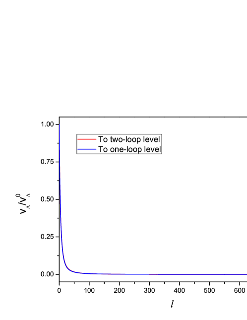
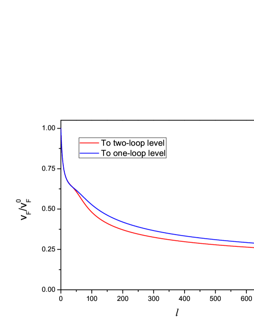
Figure 7: The running of $v_{\Delta}$ (left) and $v_{F}$ (right) without disorder at the two-loop level.

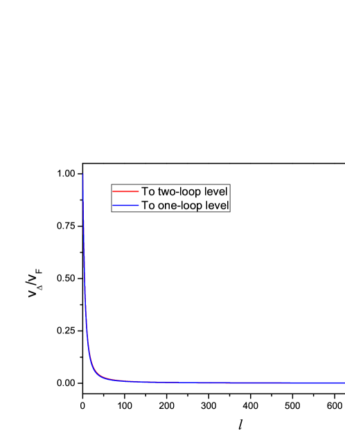
Figure 8: The running of $v_{\Delta}/v_{F}$ without disorder at the two-loop level.

IV.2 RG equation of disorder strength parameter $\zeta$

The strength parameter $v_{\Gamma}$ of random chemical potential enters into the above equations for fermion velocities. Due to the interplay of nematic fluctuation and disorder scattering, this parameter also flows under RG transformation. We calculate the two-loop diagrams for the correction to fermion-disorder vertex function and combine them with one-loop contribution, and then obtain

$$\int^{b\Lambda}d^{2}\mathbf{k}d^{2}\mathbf{k^{\prime}}d^{2}\mathbf{k^{\prime\prime}}d\omega d\omega^{\prime\prime}\psi^{\dagger}_{m}(\mathbf{k},\omega)\psi_{m}(\mathbf{k^{\prime}},\omega)\psi^{\dagger}_{n}(\mathbf{k^{\prime\prime}},\omega^{\prime\prime})$$ (50)

$$\times\psi_{n}(\mathbf{k}+\mathbf{k^{\prime\prime}}-\mathbf{k^{\prime}},\omega^{\prime\prime})\left(-\frac{\zeta}{4}\right)\Bigl{[}1-2C_{1}l+4C_{g}l+4C_{g}^{2}l^{2}$$

$$+C_{l}l^{2}+C_{1}C_{h}l^{2}+C_{g}C_{f}l^{2}+C_{k}l^{2}-2C_{g}C_{1}l^{2}+8C^{2}_{g}l^{2}$$

$$+2C^{2}_{1}l^{2}+C_{m}l^{2}-4C_{1}C_{g}l^{2}-8C_{g}^{2}l^{2}+16C_{g}^{2}l^{2}+C_{g}C_{n}l^{2}$$

$$+2C_{g}(C_{2}+C_{3})l^{2}\Bigr{]}$$

$$= \int^{\Lambda}d^{2}\mathbf{k}d^{2}\mathbf{k^{\prime}}d^{2}\mathbf{k^{\prime\prime}}d\omega d\omega^{\prime\prime}\psi^{\dagger}_{m}(\mathbf{k},\omega)\psi_{m}(\mathbf{k^{\prime}},\omega)\psi^{\dagger}_{n}(\mathbf{k^{\prime\prime}},\omega^{\prime\prime})$$

$$\times\psi_{n}(\mathbf{k}+\mathbf{k^{\prime\prime}}-\mathbf{k^{\prime}},\omega^{\prime\prime})\left(-\frac{\zeta}{4}\right)\exp\Bigl{\{}\Bigl{[}\frac{m_{1}}{3}-2C_{g}d_{1}$$

$$+12C_{g}^{2}+C_{1}C_{h}+C_{g}C_{f}+2C^{2}_{1}-8C_{1}C_{g}+C_{k}+C_{l}$$

$$+C_{m}+C_{g}C_{n}+C_{g}(C_{2}+C_{3})\Bigr{]}l^{2}\Bigr{\}}$$

$$\equiv \int^{\Lambda}d^{2}\mathbf{k}d^{2}\mathbf{k^{\prime}}d^{2}\mathbf{k^{\prime\prime}}d\omega d\omega^{\prime\prime}\psi^{\dagger}_{m}(\mathbf{k},\omega)\psi_{m}(\mathbf{k^{\prime}},\omega)\psi^{\dagger}_{n}(\mathbf{k^{\prime\prime}},\omega^{\prime\prime})$$

$$\times\psi_{n}(\mathbf{k}+\mathbf{k^{\prime\prime}}-\mathbf{k^{\prime}},\omega^{\prime\prime})\left(-\frac{\zeta^{\prime}}{4}\right),$$

where

$$\zeta^{\prime} = \zeta\exp\Bigl{\{}\Bigl{[}\frac{m_{1}}{3}-2C_{g}d_{1}+12C_{g}^{2}+C_{1}C_{h}+C_{g}C_{f}$$ (51)

$$+2C^{2}_{1}-8C_{1}C_{g}+C_{k}+C_{l}+C_{m}+C_{g}C_{n}$$

$$+C_{g}(C_{2}+C_{3})\Bigr{]}l^{2}\Bigr{\}}.$$

The RG equation for parameter $\zeta$ up to two-loop level is finally found to be

$$\frac{d\zeta}{dl} = 2l\Bigl{[}C_{g}(12C_{g}-2d_{1}+C_{f})+C_{1}(C_{h}+2C_{1}-8C_{g})+\left(\frac{m_{1}}{3}+C_{k}+C_{l}+C_{m}\right)+C_{g}(C_{n}+C_{2}+C_{3})\Bigr{]}\zeta.$$ (52)

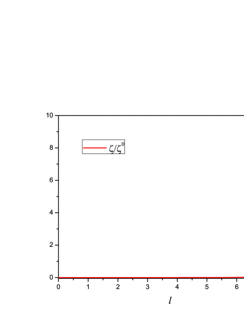
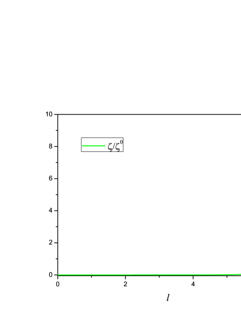
Figure 9: Flows of the disorder strength $\zeta$ with the initial values $(v_{\Delta}/v_{F})^{0}=0.1,v^{0}_{F}=1,v^{0}_{\Delta}=0.1$, $\zeta^{0}=10^{-5}$ (left) and $\zeta^{0}=10^{-4}$ (right) at the two-loop level.

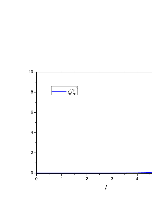
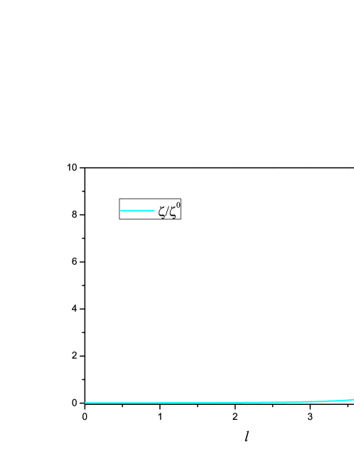
Figure 10: Flows of $\zeta$ with initial values $(v_{\Delta}/v_{F})^{0}=0.1,v^{0}_{F}=1,v^{0}_{\Delta}=0.1$, $\zeta^{0}=10^{-3}$ (left) and $\zeta^{0}=10^{-2}$ (right) at the two-loop level.

V Numerical solutions for RG equations and discussions

The RG equations for fermion velocities and disorder parameter have been derived in the last section. The aim of this section is to analyze the solutions of these equations, which are self-consistently coupled to each other and therefore need to be solved numerically. To make the discussion more transparent, we first consider the clean limit with $\zeta=0$ and then include disorder later.

V.1 Clean limit

In the clean case, $\zeta=0$, the RG equations have the following form up to two-loop level,

$$\frac{dv_{F}}{dl} = \left[C_{1}-C_{2}+\frac{(m_{1}-m_{2})}{3}l\right]v_{F},$$ (53)

$$\frac{dv_{\Delta}}{dl} = \left[C_{1}-C_{3}+\frac{(m_{1}-m_{3})}{3}l\right]v_{\Delta},$$ (54)

$$\frac{d\frac{v_{\Delta}}{v_{F}}}{dl} = \left[C_{2}-C_{3}+\frac{(m_{2}-m_{3})}{3}l\right]\frac{v_{\Delta}}{v_{F}}.$$ (55)

Solving these RG equations numerically, we find that the results qualitatively agrees with those obtained at one-loop level Ref. Huh2008PRB , which can be clearly seen from Figs. (7) and (8). In particular, $v_{F}$ vanishes with growing $l$ much more slowly than $v_{\Delta}$, so the velocity ratio $v_{\Delta}/v_{F}\rightarrow 0$ at large length scale, which corresponding to a stable fixed point of extreme anisotropy. It therefore turns out that the one-loop results are robust and that the $1/N$-expansion is fairly reliable.

V.2 In the presence of disorders

Now we consider the influence of random chemical potential. Before running into complex numerical computation, it is helpful to first make a simple analysis about the behavior of parameter $\zeta$. From the flow equation of $\zeta$ (52), it is convenient to extract a general differential equation, $\frac{d\zeta}{dl}=Cl\zeta$. Apparently, the fate of $\zeta$ in the low-energy region (i.e., large $l$ limit) is unambiguously determined by the value of the coefficient $C$: as the running length scale $l$ increases, $\zeta$ flows towards infinity, vanishes, and stays at a certain constant for $C>0$, $C<0$, and $C=0$, respectively. Previous one-loop calculations Stauber2005PRB ; WLK2011PRB showed that the coefficient $C$ vanishes, so the strength parameter $\zeta$ of random chemical potential is marginal and remains a constant as $l$ varies. After including two-loop corrections, $C$ may become either positive or negative, which will be addressed by solving the coupled flow equations (47), (48), (49), and (52).

The numerical solutions of RG equations with properly chosen initial values of disorder parameter are shown in Figs. 9 and 10. As $l$ grows, $\zeta$ increases quickly and eventually diverges in the limit $l\rightarrow+\infty$. This behavior does not depend on the initial values of the running parameters. Therefore, the strength parameter of random chemical potential, which is marginal at one-loop level, becomes relevant after including the two-loop order corrections. This change may have significant influence on the physical properties of the system under consideration since even an infinitesimal relevant parameter will flow to very large at ultra low energies.

A natural question arises: how can we understand the marginally relevant nature of the characteristic parameter $\zeta$ of random chemical potential and its impacts on the nematic quantum criticality in $d$-wave superconductors? In the clean limit, $\zeta=0$, the strong quantum fluctuation of nematic order results in non-Fermi liquid behavior of nodal fermions Kim2008PRB ; Liu2015 . Once random chemical potential is introduced, the non-Fermi liquid state is immediately turned into a diffusive metallic state Fradkin1986PRB ; Lee1993PRL ; Foster2008PRB ; Shindou2009PRB ; Moon2014 ; Ominato2014PRB ; Goswami2011PRL ; Kobayashi2014PRL ; Sbierski2014PRL ; Lai_Roy2014 , which has a finite zero-energy density of states and finite scattering rate. This conclusion is valid for all possible values of $\zeta$, since $\zeta$, irrespective of its initial value, unavoidably flows to infinity in the low-energy regime.

VI Physical implications

In addition to the tendency of non-Fermi liquid behavior due to the marginally relevant behavior of random chemical potential, we, within this section, try to delineate investigate the influence of nematic fluctuation, gapless QPs and marginally relevant random chemical potential on a number of significantly physical observables in a $d$-wave cuprate superconductor at the nematic QCP, such as the superfluid density, critical temperature, and thermal conductivity.

Learning from the Fig. 9 and the discussion in Sec. V, we can be recalled some points. On the one hand, the strength of random chemical potential, due to the marginally relevant behavior, flows away with the energy scale $l$ reaching a critical value, dubbed $l^{*}$, at the nematic QCP. This indirectly triggers the unphyscial behaviors of fermion velocities $v_{F}$ and $v_{\Delta}$ at a very scale $l=l^{*}$ which is dependent on the initial values of $v_{F}$ and $v_{\Delta}$ by the growing strength of random chemical potential and will be carefully investigated in the following subsections. On the other hand, runaway behavior of physical quantities suggests a first-order phase transition Domany1977PRB ; Chen1978PRB ; Rudnick1978PRB ; Iacobson1981AP ; Cardybook . In order to figuratively describe it in finite temperatures, we employ a useful formula $T=T_{c}e^{-l}$ Huh2008PRB ; She2014 ($T_{c}$ is the critical temperature of superconductor) to translate $l^{*}$ to $T^{*}$.

It is necessary to further emphasize that our effective theory and method are only valid for the continuous phase transitions and hence we subsequently focus on the critical behaviors of physical observables with the confined region $T>T^{*}$, such as superfluid density, critical temperature and thermal conductivity.

VI.1 Superfluid density and critical temperature

As studied by Lee and Wen Lee1997PRL , the superfluid density in the noninteracting case exhibits a linear temperature dependence which is in agreement with experiments Hardy1993PRL

$$\frac{\rho_{s}(T)}{m}=\frac{\rho_{s}(0)}{m}-\frac{2\ln 2}{\pi}\frac{v_{F}}{v_{\Delta}}T,$$ (56)

with $\rho_{s}(0)=\frac{x}{a^{2}}$ where $x$ and $a$ represent the doping concentration and lattice spacing, respectively and $T_{c}\propto\frac{v_{\Delta}}{v_{F}}\frac{x}{ma^{2}}$ by defining $\rho_{s}(T_{c})=0$, reproducing the Uemura plot Uemura1989PRL . The other term of right hand side is the contribution of the normal QPs density. As presented in the previous section, the fermion velocities $v_{F}$, $v_{\Delta}$, and the ratio $v_{\Delta}/v_{F}$ are heavily renormalized by the interplay between nematic fluctuation and the effects of random chemical potential in the vicinity of the nematic QCP. We can approximately derive the superfluid density of of the $d$-wave superconducting state at the nematic QCP which is renormalized by nematic fluctuation and marginally relevant random chemical potential Lee1997PRL ; Durst2000PRB ,

$$\rho^{\prime}_{s}(T)=\rho_{s}(0)-\rho_{n}(T),$$ (57)

where the normal QPs density is complicatedly dependent on the fermion velocities $v_{F}$ and $v_{\Delta}$

$$\frac{\rho_{n}(T)}{m}=\frac{4}{k_{B}T}\int\frac{d^{2}\mathbf{k}}{(2\pi)^{2}}\frac{v_{F}^{2}(\mathbf{k})e^{\frac{\sqrt{v_{F}^{2}(\mathbf{k})k_{x}^{2}+v_{\Delta}^{2}(\mathbf{k})k_{y}^{2}}}{k_{B}T}}}{\left(1+e^{\frac{\sqrt{v_{F}^{2}(\mathbf{k})k_{x}^{2}+v_{\Delta}^{2}(\mathbf{k})k_{y}^{2}}}{k_{B}T}}\right)^{2}}.$$ (58)

By combing the Eqs. (57) and (58) and Eqs. (47), (48), and (49), the superfluid density and critical temperature are dependent on the running of velocities $v_{F}$ and $v_{\Delta}$ and also the behavior of disorder which is coupled with the velocities $v_{F}$ and $v_{\Delta}$ as lineated by Eqs. (47), (48), and (49). To include these corrections and after some numerical calculations, we obtain the $\rho^{\prime}_{s}(T)/\rho_{s}(T)$ with the different initial values of fermion velocities $v_{F}$ and $v_{\Delta}$ for $T>T^{*}$ as depicted in Fig. 11.

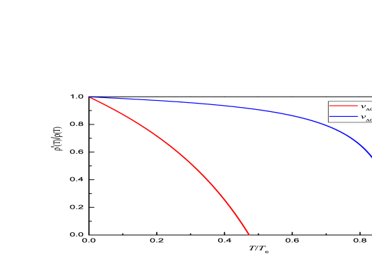
Figure 11: Temperature-dependence superfluid density in the presence of the nematic fluctuation and random chemical potential at nematic QCP for the representatively initial values of $v_{\Delta}/v_{F}$ and random chemical potential. The primary conclusions are independent of the initial values.

Studying from the numerical results in Fig. 11, we can draw a conclusion that the superfluid density and critical temperature are largely suppressed in the presence of marginally relevant random chemical potential nearby the nematic QCP. This may be very instructive to provide another clue to locate the nematic QCP.

VI.2 Thermal conductivity

We then turn to the thermal conductivity of QPS. By paralleling the derivations in Ref. Durst2000PRB , we obtain the thermal conductivity of QPs for the constant values of fermion velocities $v_{F}$ and $v_{\Delta}$,

$$\frac{\kappa}{T} = \frac{k^{2}_{B}}{3}\left(\frac{v_{f}}{v_{\Delta}}+\frac{v_{\Delta}}{v_{f}}\right),$$ (59)

and for the energy scale-dependence $v_{F}$ and $v_{\Delta}$ which are comprised the nematic fluctuation and marginally relevant random chemical potential in the vicinity of nematic QCP,

$$\frac{\kappa^{\prime}}{T} = \left(\frac{k^{2}_{B}}{3}\right)\int^{\frac{\Lambda_{0}}{\zeta_{0}}}_{0}\!\!\frac{d\mathbf{k}}{\left(1+\mathbf{k}^{2}\right)^{2}}\left[\frac{v_{F}(\mathbf{k})}{v_{\Delta}(\mathbf{k})}+\frac{v_{\Delta}(\mathbf{k})}{v_{F}(\mathbf{k})}\right]\!,$$ (60)

with $\Lambda_{0}$ determined by the lattice constant and $\zeta_{0}$ the initial value of disorder strength. In order to examine the influence of nematic fluctuation and random chemical potential, we numerically carry out the Eqs. (47), (48), (49), (59) and (60) and reach the numerical results as presented for $T>T^{*}$ in Fig. 12.

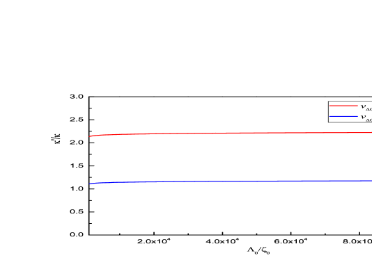
Figure 12: Thermal conductivity of QPS in the presence of nematic fluctuation and random chemical potential at nematic QCP for the representatively initial values of $v_{\Delta}/v_{F}$ and random chemical potential. The primary conclusions are independent of the initial values.

As exhibited in Fig. 12, the thermal conductivity of QPs, influenced by nematic fluctuation and marginally relevant random chemical potential at the nematic QCP, is highly increased and insensitive to the initial values of random chemical potential. This may be helpful to enhance our understand the phase diagram of $d$-wave superconductors.

VII Summary

In summary, we have investigated the impact of a particular disorder, namely random chemical potential, on the stability of nematic quantum critical point located in the superconducting dome of $d$-wave superconductors. We performed a detailed RG analysis up to two-loop order within an effective field theory that describes the interplay of nematic fluctuation and disorder scattering. The effective parameter that characterize the strength of random chemical potential is marginal at one-loop order, but becomes relevant due to the inclusion of two-loop order corrections. This means that, even if we start from a very weak disorder, the effective strength of disorder eventually becomes infinitely large at the lowest energy. The Dirac fermions therefore enter into a diffusive metallic state driven by random chemical potential at the nematic quantum critical point Fradkin1986PRB ; Shindou2009PRB ; Ominato2014PRB ; Goswami2011PRL ; Kobayashi2014PRL ; Sbierski2014PRL . Furthermore, we carefully study the critical behaviors for a number of significantly physical observables in a $d$-wave cuprate superconductor at the nematic QCP, such as the superfluid density, critical temperature, and thermal conductivity in the vicinity of nematic QCP.

Appendix A Some coefficients used in the main text

The coefficients for one-loop Feynman diagrams are

$$C_{1} = \frac{2v_{\Delta}}{N_{f}\pi^{3}v_{F}}\int^{\infty}_{-\infty}dx\int^{2\pi}_{0}d\theta\frac{x^{2}-\cos^{2}\theta-\left(\frac{v_{\Delta}}{v_{F}}\right)^{2}\sin^{2}\theta}{\left[x^{2}+\cos^{2}\theta+\left(\frac{v_{\Delta}}{v_{F}}\right)^{2}\sin^{2}\theta\right]^{2}}\mathcal{G}(x,\theta),$$ (61)

$$C_{2} = \frac{2v_{\Delta}}{N_{f}\pi^{3}v_{F}}\int^{\infty}_{-\infty}dx\int^{2\pi}_{0}d\theta\frac{\cos^{2}\theta-x^{2}-\left(\frac{v_{\Delta}}{v_{F}}\right)^{2}\sin^{2}\theta}{\left[x^{2}+\cos^{2}\theta+\left(\frac{v_{\Delta}}{v_{F}}\right)^{2}\sin^{2}\theta\right]^{2}}\mathcal{G}(x,\theta),$$ (62)

$$C_{3} = \frac{2v_{\Delta}}{N_{f}\pi^{3}v_{F}}\int^{\infty}_{-\infty}dx\int^{2\pi}_{0}d\theta\frac{x^{2}+\cos^{2}\theta-\left(\frac{v_{\Delta}}{v_{F}}\right)^{2}\sin^{2}\theta}{\left[x^{2}+\cos^{2}\theta+\left(\frac{v_{\Delta}}{v_{F}}\right)^{2}\sin^{2}\theta\right]^{2}}\mathcal{G}(x,\theta),$$ (63)

$$\mathcal{G}^{-1} = \frac{x^{2}+\cos^{2}\theta}{\sqrt{x^{2}+\cos^{2}\theta+\left(\frac{v_{\Delta}}{v_{F}}\right)^{2}\sin^{2}\theta}}+\frac{x^{2}+\sin^{2}\theta}{\sqrt{x^{2}+\sin^{2}\theta+\left(\frac{v_{\Delta}}{v_{F}}\right)^{2}\cos^{2}\theta}},$$ (64)

and

$$C_{g}=-\frac{\zeta}{4}\frac{1}{2\pi v_{F}v_{\Delta}}.$$ (65)

For two-loop Feynman diagrams, the corresponding coefficients are

$$m_{1} = \frac{2v_{\Delta}}{N_{f}\pi^{3}v_{F}}\int^{\infty}_{-\infty}dx\int^{2\pi}_{0}d\theta\frac{\mathcal{G}(x,\theta)}{\left[x^{2}+\cos^{2}\theta+\left(\frac{v_{\Delta}}{v_{F}}\right)^{2}\sin^{2}\theta\right]^{3}}$$ (66)

$$\times\left\{4x^{2}\left[C_{1}x^{2}+(2C_{2}-C_{1})\cos^{2}\theta+(2C_{3}-C_{1})\left(\frac{v_{\Delta}}{v_{F}}\right)^{2}\sin^{2}\theta\right.\right]$$

$$-\left[3C_{1}x^{2}+(2C_{2}-C_{1})\cos^{2}\theta+(2C_{3}-C_{1})\left(\frac{v_{\Delta}}{v_{F}}\right)^{2}\sin^{2}\theta\right]$$

$$\left.\times\left[x^{2}+\cos^{2}\theta+\left(\frac{v_{\Delta}}{v_{F}}\right)^{2}\sin^{2}\theta\right]\right\},$$

$$m_{2} = \frac{2v_{\Delta}}{N_{f}\pi^{3}v_{F}}\int^{\infty}_{-\infty}dx\int^{2\pi}_{0}d\theta\frac{\mathcal{G}(x,\theta)}{\left[x^{2}+\cos^{2}\theta+\left(\frac{v_{\Delta}}{v_{F}}\right)^{2}\sin^{2}\theta\right]^{3}}$$ (67)

$$\times\left\{\left[(C_{2}-2C_{1})x^{2}+(C_{2}-2C_{3})\left(\frac{v_{\Delta}}{v_{F}}\right)^{2}\sin^{2}\theta-3C_{2}\cos^{2}\theta\right]\right.$$

$$\times\left[x^{2}+\cos^{2}\theta+\left(\frac{v_{\Delta}}{v_{F}}\right)^{2}\sin^{2}\theta\right]-4\cos^{2}\theta\Bigl{[}(C_{2}-2C_{1})x^{2}$$

$$\left.+(C_{2}-2C_{3})\left(\frac{v_{\Delta}}{v_{F}}\right)^{2}\sin^{2}\theta-C_{2}\cos^{2}\theta\Bigr{]}\right\},$$

$$m_{3} = \frac{2v_{\Delta}}{N_{f}\pi^{3}v_{F}}\int^{\infty}_{-\infty}dx\int^{2\pi}_{0}d\theta\frac{\mathcal{G}(x,\theta)}{\left[x^{2}+\cos^{2}\theta+\left(\frac{v_{\Delta}}{v_{F}}\right)^{2}\sin^{2}\theta\right]^{3}}$$ (68)

$$\times\left\{\left[3C_{3}\left(\frac{v_{\Delta}}{v_{F}}\right)^{2}\sin^{2}\theta+(2C_{2}+C_{3})\cos^{2}\theta+(2C_{1}-C_{3})x^{2}\right]\right.$$

$$\times\left[x^{2}+\cos^{2}\theta+\left(\frac{v_{\Delta}}{v_{F}}\right)^{2}\sin^{2}\theta\right]-4\left(\frac{v_{\Delta}}{v_{F}}\right)^{2}\sin^{2}\theta\Bigl{[}(2C_{1}-C_{3})x^{2}$$

$$\left.+C_{3}\left(\frac{v_{\Delta}}{v_{F}}\right)^{2}\sin^{2}\theta+(2C_{2}+C_{3})\cos^{2}\theta\Bigr{]}\right\},$$

$$d_{1} = \frac{2v_{\Delta}}{N_{f}\pi^{3}v_{F}}\int^{\infty}_{-\infty}dx\int^{2\pi}_{0}d\theta\frac{\mathcal{G}(x,\theta)}{\left[x^{2}+\cos^{2}\theta+\left(\frac{v_{\Delta}}{v_{F}}\right)^{2}\sin^{2}\theta\right]^{3}}$$ (69)

$$\times\left\{\left[3x^{2}-\cos^{2}\theta-\left(\frac{v_{\Delta}}{v_{F}}\right)^{2}\sin^{2}\theta\right]\left[x^{2}+\cos^{2}\theta+\left(\frac{v_{\Delta}}{v_{F}}\right)^{2}\sin\theta^{2}\right]\right.$$

$$\left.-4x^{2}\left[x^{2}-\cos^{2}\theta-\left(\frac{v_{\Delta}}{v_{F}}\right)^{2}\sin^{2}\theta\right]\right\},$$

$$d_{2} = \frac{4v_{\Delta}}{N_{f}\pi^{3}v_{F}}\int^{\infty}_{-\infty}dx\int^{2\pi}_{0}d\theta\frac{x^{2}\mathcal{G}(x,\theta)}{\left[x^{2}+\cos^{2}\theta+\left(\frac{v_{\Delta}}{v_{F}}\right)^{2}\sin^{2}\theta\right]^{3}}$$ (70)

$$\times\left[x^{2}+\left(\frac{v_{\Delta}}{v_{F}}\right)^{2}\sin^{2}\theta-3\cos^{2}\theta\right],$$

$$d_{3} = -\frac{4v_{\Delta}}{N_{f}\pi^{3}v_{F}}\int^{\infty}_{-\infty}dx\int^{2\pi}_{0}d\theta\frac{x^{2}\mathcal{G}(x,\theta)}{\left[x^{2}+\cos^{2}\theta+\left(\frac{v_{\Delta}}{v_{F}}\right)^{2}\sin^{2}\theta\right]^{3}}$$ (71)

$$\times\left[x^{2}+\cos^{2}\theta-3\left(\frac{v_{\Delta}}{v_{F}}\right)^{2}\sin^{2}\theta\right],$$

$$C_{h} = -\frac{2v_{\Delta}}{3N_{f}\pi^{3}v_{F}}\int^{\infty}_{-\infty}dx\int^{2\pi}_{0}d\theta\frac{\left(\frac{v_{\Delta}}{v_{F}}\right)^{2}\sin^{2}\theta\mathcal{G}(x,\theta)}{\left[x^{2}+\cos^{2}\theta+\left(\frac{v_{\Delta}}{v_{F}}\right)^{2}\sin^{2}\theta\right]^{2}},$$ (72)

$$C_{f} = -\frac{4v_{\Delta}}{N_{f}\pi^{3}v_{F}}\int^{\infty}_{-\infty}dx\int^{2\pi}_{0}d\theta\frac{\mathcal{G}(x,\theta)}{\left[x^{2}+\cos^{2}\theta+\left(\frac{v_{\Delta}}{v_{F}}\right)^{2}\sin^{2}\theta\right]^{2}}$$ (73)

$$\times\left[x^{2}-\cos^{2}\theta-\left(\frac{v_{\Delta}}{v_{F}}\right)^{2}\sin^{2}\theta\right],$$

$$C_{k} = \frac{2\sqrt{3\pi}v_{F}v_{\Delta}}{9N_{f}^{2}\pi^{3}}\int^{\infty}_{-\infty}dx\int^{2\pi}_{0}d\theta\frac{\mathcal{G}(x,\theta)}{\left[x^{2}+\cos^{2}\theta+\left(\frac{v_{\Delta}}{v_{F}}\right)^{2}\sin^{2}\theta\right]}$$ (74)

$$\times\left[E_{1}x^{2}-E_{2}\cos^{2}\theta+E_{3}\left(\frac{v_{\Delta}}{v_{F}}\right)^{2}\sin^{2}\theta\right],$$

$$C_{l} = \frac{\zeta}{N_{f}\pi^{4}v_{F}^{2}}\int^{\infty}_{-\infty}dx\int^{2\pi}_{0}d\theta\frac{\mathcal{G}(x,\theta)}{\left[x^{2}+\cos^{2}\theta+\left(\frac{v_{\Delta}}{v_{F}}\right)^{2}\sin^{2}\theta\right]},$$ (75)

$$C_{m} = \frac{4v_{\Delta}}{3N_{f}\pi^{3}v_{F}}\int^{\infty}_{-\infty}dx\int^{2\pi}_{0}d\theta\frac{\mathcal{G}(x,\theta)}{\left[x^{2}+\cos^{2}\theta+\left(\frac{v_{\Delta}}{v_{F}}\right)^{2}\sin^{2}\theta\right]^{3}}$$ (76)

$$\times\left\{C_{3}\left(\frac{v_{\Delta}}{v_{F}}\right)^{4}\sin^{4}\theta+3(C_{1}+C_{2})x^{2}\cos^{2}\theta-C_{2}\cos^{4}\theta-C_{1}x^{4}\right.$$

$$\left.+\left(\frac{v_{\Delta}}{v_{F}}\right)^{2}\sin^{2}\theta\left[3(C_{1}-C_{3})x^{2}+(C_{3}-C_{2})\cos^{2}\theta\right]\right\},$$

$$C_{n} = \frac{8v_{\Delta}}{N_{f}\pi^{3}v_{F}}\int^{\infty}_{-\infty}dx\int^{2\pi}_{0}d\theta\frac{x^{2}\mathcal{G}(x,\theta)}{\left[x^{2}+\cos^{2}\theta+\left(\frac{v_{\Delta}}{v_{F}}\right)^{2}\sin^{2}\theta\right]^{3}}$$ (77)

$$\times\left[x^{2}-3\cos^{2}\theta-3\left(\frac{v_{\Delta}}{v_{F}}\right)^{2}\sin^{2}\theta\right],$$

with

$$E_{1} = \frac{8\sqrt{2}v_{\Delta}}{\pi^{5/2}v_{F}^{3}}\int^{\infty}_{-\infty}dy\int^{2\pi}_{0}d\varphi\frac{\mathcal{G}(y,\varphi)}{\left[y^{2}+\cos^{2}\varphi+\left(\frac{v_{\Delta}}{v_{F}}\right)^{2}\sin^{2}\varphi\right]^{4}}$$ (78)

$$\times\left\{\left[y^{2}+\cos^{2}\varphi-\left(\frac{v_{\Delta}}{v_{F}}\right)^{2}\sin^{2}\varphi\right]\left[y^{2}+\left(\frac{v_{\Delta}}{v_{F}}\right)^{2}\sin^{2}\varphi+\cos^{2}\varphi\right]\right.$$

$$\left.-2y^{2}\left[y^{2}+\cos^{2}\varphi-3\left(\frac{v_{\Delta}}{v_{F}}\right)^{2}\sin^{2}\varphi\right]\right\},$$

$$E_{2} = \frac{8\sqrt{2}v_{\Delta}}{\pi^{5/2}v_{F}^{3}}\int^{\infty}_{-\infty}dy\int^{2\pi}_{0}d\varphi\frac{(\cos^{2}\varphi-y^{2})\mathcal{G}(y,\varphi)}{\left[y^{2}+\cos^{2}\varphi+\left(\frac{v_{\Delta}}{v_{F}}\right)^{2}\sin^{2}\varphi\right]^{3}},$$ (79)

$$E_{3} = \frac{8\sqrt{2}v_{\Delta}}{\pi^{5/2}v_{F}^{3}}\int^{\infty}_{-\infty}dy\int^{2\pi}_{0}d\varphi\frac{\mathcal{G}(y,\varphi)}{\left[y^{2}+\cos^{2}\varphi+\left(\frac{v_{\Delta}}{v_{F}}\right)^{2}\sin^{2}\varphi\right]^{4}}$$ (80)

$$\times\left\{\left[\left(\frac{v_{\Delta}}{v_{F}}\right)^{2}\sin^{2}\varphi-y^{2}\right]\left[\left(\frac{v_{\Delta}}{v_{F}}\right)^{2}\sin^{2}\varphi+\cos^{2}\varphi+y^{2}\right]\right.$$

$$\left.+2\left(\frac{v_{\Delta}}{v_{F}}\right)^{2}\sin^{2}\varphi\left[3y^{2}-\cos^{2}\varphi-\left(\frac{v_{\Delta}}{v_{F}}\right)^{2}\sin^{2}\varphi\right]\right\}.$$

References

- (1) Orenstein J and Millis A J 2000 Science 288 468
- (2) Vojta M 2009 Adv. Phys. 58 699
- (3) Ando Y, Segawa K, Komiya S, and Lavrov A N 2002 Phys. Rev. Lett. 88 137005
- (4) Hinkov V, Haug D, Fauque B, Bourges P, Sidis Y, Ivanov A, Bernhard C, Lin C T, and Keimer B 2008 Science 319 597
- (5) Daou R, Chang J, LeBoeuf D, Cyr-Choiniere O, Laliberte F, Doiron-Leyraud N, Ramshaw B J, Liang R, Bonn D A, Hardy W N, and Taillefer L 2010 Nature (London) 463 519
- (6) Lawler M J, Fujita K, Lee J, Schmidt A R, Kohsaka Y, Kim C K, Eisaki H, Uchida S, Davis J C, Sethna J P, and Kim E-A 2010 Nature 466 347
- (7) Borzi R A, Grigera S A, Farrell J, Perry R S, Lister S J, Lee S L, Tennant D A, Maeno Y, and Mackenzie A P 2007 Science 315 214
- (8) Chuang T-M, Allan M P, Lee J, Xie Y, Ni N, Bud’ko S L, Boebinger G S, Canfield P C, and Davis J C 2010 Science 327 181
- (9) Kivelson S A, Fradkin E, and Emery V J 1998 Nature (London) 393 550
- (10) Yamase H and Kohno H 2000 J. Phys. Soc. Jpn. 69 332; 2000 J. Phys. Soc. Jpn. 69 2151
- (11) Halboth C J and Metzner W 2000 Phys. Rev. Lett. 85 5162
- (12) Fradkin E, Kivelson S A, Lawler M J, Eisenstein J P, and Mackenzie A P 2010 Annu. Rev. Condens. Matter Phys. 1 153
- (13) Sachdev S 1999 Quantum phase transitions (Cambridge University Press, Cambridge)
- (14) Yamase H and Metzner W 2007 Phys. Rev. B 75 155117
- (15) Zhang Y, Demler E, and Sachdev S 2002 Phys. Rev. B 66 094501
- (16) Raghu S, Paramekanti A, Kim E-A, Borzi R A, Grigera S, Mackenzie A P, Kivelson S A 2009 Phys. Rev. B 79 214402
- (17) Moon E G and Sachdev S 2010 Phys. Rev. B 82 104516
- (18) Vojta M, Zhang Y, and Sachdev S 2000 Phys. Rev. Lett. 85 4940
- (19) Vojta M, Zhang Y, and Sachdev S 2000 Phys. Rev. B 62 6721
- (20) Vojta M, Zhang Y, and Sachdev S 2000 Int. J. Mod. Phys. B 14 3719
- (21) Khveshchenko D V and Paaske J 2001 Phys. Rev. Lett. 86 4672
- (22) Kim E-A, Lawler M J, Oreto P, Sachdev S, Fradkin E, and Kivelson S A 2008 Phys. Rev. B 77 184514
- (23) Oganesyan V, Kivelson S A, and Fradkin E 2001 Phys. Rev. B 64 195109
- (24) Huh Y and Sachdev S 2008 Phys. Rev. B 78 064512
- (25) Xu C, Qi Y, and Sachdev S 2008 Phys. Rev. B 78 134507
- (26) Fritz L and Sachdev S 2009 Phys. Rev. B 80 144503
- (27) Liu G-Z, Wang J-R, and Wang J 2012 Phys. Rev. B 85 174525
- (28) Wang J-R and Liu G-Z 2013 New J. Phys. 15 063007
- (29) She J-H, Lawler M J, and Kim E-A 2014 arXiv:cond-mat/1410.5365
- (30) Liu G-Z, Wang J-R, and Zhang C-J 2015 in preparation
- (31) Lee P A and Ramakrishnan T V 1985 Rev. Mod. Phys. 57 287
- (32) Altland A, Simons B D, and Zirnbauer M R 2002 Phys. Rep. 359 283
- (33) Lee P A, Nagaosa N, and Wen X-G, 2006 Rev. Mod. Phys. 78 17
- (34) Novoselov K S, Geim A K, Morozov S V, Jiang D, Katsnelson M I, Grigorieva I V, Dubonos S V, and Firsov A A 2005 Nature 438 197
- (35) Aleiner I L and Efetov K B 2006 Phys. Rev. Lett. 97 236801
- (36) Foster M S and Aleiner I L 2006 Phys. Rev. Lett. 77 195413
- (37) Castro Neto A H, Guinea F, Peres N M R, Novoselov K S, and Geim A K 2009 Rev. Mod. Phys. 81 109
- (38) S Das Sarma, Adam S, Hwang E H, and Rossi E 2011 Rev. Mod. Phys. 83 407
- (39) Kotov V N, Uchoa B, Pereira V M, Guinea F, and Castro Neto A H 2012 Rev. Mod. Phys. 84 1067
- (40) Ludwig A W W, Fisher M P A, Shankar R, and Grinstein G 1994 Phys. Rev. B 50 7526
- (41) Furneaux J E, Kravchenko S V, Mason W E, Bowker G E, and Pudalov V M 1995 Phys. Rev. B 51 17227
- (42) Ye J and Sachdev S 1998 Phys. Rev. Lett. 80 5409; Ye J 1999 Phys. Rev. B 60 8290
- (43) Hasan M Z and Kane C L 2010 Rev. Mod. Phys. 82 3045
- (44) Nersesyan A A, Tsvelik A M, and Wenger F 1995 Nucl. Phys. B 438 561
- (45) Stauber T, Guinea F, and Vozmediano M A H 2005 Phys. Rev. B 71 041406
- (46) Wang J, Liu G-Z, and Kleinert H 2011 Phys. Rev. B 83 214503
- (47) Wang J 2013 Phys. Rev. B 87 054511
- (48) Wilson K G 1975 Rev. Mod. Phys. 47 773
- (49) Polchinski J 1992 arXiv:hep-th/9210046
- (50) Shankar R 1994 Rev. Mod. Phys. 66 129
- (51) Roy B and Das Sarma S 2014 Phys. Rev. B 90 241112(R)
- (52) Edwards S and Anderson P W 1975 J. Phys. F 5 965
- (53) Lerner I V 2003 arXiv:cond-mat/0307471
- (54) Wang J and Liu G-Z 2013 New J. Phys. 15 073039
- (55) Mishchenko E G 2007 Phys. Rev. Lett. 98 216801
- (56) Vafek O and Case M J 2008 Phys. Rev. B 77 033410
- (57) Fradkin E 1986 Phys. Rev. B 33 3257; Phys. Rev. B 33 3263
- (58) Lee P A 1993 Phys. Rev. Lett. 71 3257
- (59) Foster M S and Aleiner I L 2008 Phys. Rev. B 77 195413
- (60) Moon E-G and Kim Y B 2014 arXiv: 1409.0573
- (61) Shindou R and Murakami S 2009 Phys. Rev. B 79 045321
- (62) Ominato Y and Koshino M 2014 Phys. Rev. B 89 054202
- (63) Goswami P and Chakravarty S 2011 Phys. Rev. Lett. 107 196803
- (64) Kobayashi K, Ohtsuki T, Imura K-I, and Herbut I F 2014 Phys. Rev. Lett. 112 016402
- (65) Sbierski B, Pohl G, Bergholtz E J, and Brouwer P W 2014 Phys. Rev. Lett. 113 026602
- (66) Lai H-H, Roy B, and Goswami P 2014 arXiv: 1409.8675
- (67) Domany E, Mukamel D, and Fisher M E 1977 Phys. Rev. B 15 5432
- (68) Chen J H, Lubensky T C, and Nelson D R 1978 Phys. Rev. B 17 4274
- (69) Rudnick J 1978 Phys. Rev. B 18 1406
- (70) Iacobson H H and Amit D J 1981 Ann. Phys. 133 57
- (71) Cardy J 1996 Scaling and Renormalization in Statistical Physics (Cambridge University Press, Cambridge)
- (72) Lee P A and Wen X -G 1997 Phys. Rev. Lett. 78 4111
- (73) Durst A C and Lee P A 2000 Phys. Rev. B 62 1270
- (74) Hardy W N, Bonn D A, Morgan D C, Liang R, and Zhang K 1993 Phys. Rev. Lett. 70 3999
- (75) Uemura Y J, Luke G M, Sternlieb B J, Brewer J H, Carolan J F, Hardy W N, Kadono R, Kempton J R, Kief R F, Kreitzman S R, Mulhern P, Riseman T M, Williams D L, Yang B X, Uchida S, Takagi H, Gopalakrishnan J, Sleight A W, Subramanian M A, Chien C L, Cieplak M Z, Xiao G, Lee V Y, Statt B W, Stronach C E, Kossler W J, and Yu X H 1989 Phys. Rev. Lett. 62 2317