Explicit formula for the Holevo bound for two-parameter qubit-state estimation problem

Abstract

The main contribution of this paper is to derive an explicit expression for the fundamental precision bound, the Holevo bound, for estimating any two-parameter family of qubit mixed-states in terms of quantum versions of Fisher information. The obtained formula depends solely on the symmetric logarithmic derivative (SLD), the right logarithmic derivative (RLD) Fisher information, and a given weight matrix. This result immediately provides necessary and sufficient conditions for the following two important classes of quantum statistical models; the Holevo bound coincides with the SLD Cramér-Rao bound and it does with the RLD Cramér-Rao bound. One of the important results of this paper is that a general model other than these two special cases exhibits an unexpected property: The structure of the Holevo bound changes smoothly when the weight matrix varies. In particular, it always coincides with the RLD Cramér-Rao bound for a certain choice of the weight matrix. Several examples illustrate these findings.

I Introduction

One of the fundamental questions in quantum statistical inference problem is to establish the ultimate precision bound for a given quantum statistical model allowed by the laws of statistics and quantum theory. Mainly due to the non-commutativity of operators and nontrivial optimization over all possible measurements, this question still remains open in full generality. This is very much in contrast to the classical case where the precision bounds are obtained in terms of information quantities for various statistical inference problems.

The problem of point estimation of quantum parametric models is of fundamental importance among various quantum statistical inference problems. This problem was initiated by Helstrom in the 1960s and he devised a method to translate the well-known strategies developed in classical statistics into the quantum case helstrom . A quantum version of Fisher information was successfully introduced and the corresponding precision bound, a quantum version of Cramér-Rao (CR) bound, was derived. It turned out, however, that the obtained bound is not generally achievable except for trivial cases.

A clear distinction regarding the quantum parameter estimation problem arises when exploring possible estimation strategies since there is no measurement degrees of freedom in the classical estimation problem. Consider $n$ identical copies of a given quantum state and we are allowed to perform any kinds of quantum measurements according to quantum theory. A natural question is then to ask how much can one improve estimation errors by measurements jointly performed on the $n$ copies when compared to the case by those individually performed on each quantum state. The former class of measurements is called collective or joint and the latter is referred to as separable in literature. It is clear that the class of collective measurements includes separable ones and one expects that collective measurements should be more powerful than separable ones in general. Since one cannot do better than the best collective measurement, the ultimate precision bound is the one that is asymptotically achieved by a sequence of the best collective measurements as the number of copies tends to infinity. This fundamental question has been addressed by several authors before nagaoka89-2 ; HM98 ; GM00 ; BNG00 ; hayashi03 ; hayashi ; bbmr04 ; bbgmm06 ; HM08 ; GK06 ; KG09 ; YFG13 ; GG13 .

It was Holevo who developed parameter estimation theory of quantum states by departing from a direct analogy to classical statistics. He proposed a bound, known as the Holevo bound, in the 1970s aiming to derive the fundamental precision limit for quantum parameter estimation problem, see Ch. 6 of his book holevo . At that time, it was not entirely clear whether or not this bound is a really tight one, i.e., the asymptotic achievability by some sequence of measurements. Over the last decade, there have been several important progress on asymptotic analysis of quantum parameter estimation theory revealing that the Holevo bound is indeed the best asymptotically achievable bound under certain conditions HM08 ; GK06 ; KG09 ; YFG13 . These results confirm that the Holevo bound plays a pivotal role in the asymptotic theory of quantum parameter estimation problem. Despite the fact that we now have the fundamental precision bound, the Holevo bound has a major drawback: It is not an explicit form in terms of a given model, but rather it is written as an optimization of a certain nontrivial function. Therefore, unlike the classical case, where the Fisher information can be directly calculated from a given statistical model, the structure of this bound is not transparent in terms of the model under consideration.

Having said the above introductory remarks, we wish to gain a deeper insight into the structure of the Holevo bound reflecting statistical properties of a given model. To make progress along this line of thoughts, we take the simplest quantum parametric model, a general qubit model, and analyze its Holevo bound in detail. Since explicit formulas for the Holevo bound for mixed-state models with one and three parameters and pure-state models are known in literature, the case of two-parameter qubit model is the only one left to be solved. The main contribution of this paper is to derive an explicit expression for the Holevo bound for any two-parameter qubit model of mixed-states without referring to a specific parametrization of the model. Remarkably, the obtained formula depends solely on a given weight matrix and three previously known bounds: The symmetric logarithmic derivative (SLD) CR bound, the right logarithmic derivative (RLD) CR bound, and the bound for D-invariant models. This result immediately provides necessary and sufficient conditions for the two important cases. One is when the Holevo bound coincides with the RLD CR bound and the other is when it does with the SLD CR bound. We also show that a general model other than these two special cases exhibits an unexpected property, that is, the structure of the Holevo bound changes smoothly when the weight matrix varies. We note that similar transition has been obtained by others HM08 ; YFG13 for a specific parametrization of two-parameter qubit model. Here we emphasize that our result is most general and is expressed in terms only of the weight matrix and two quantum Fisher information.

The main result of this paper is summarized in the following theorem (The detail of these quantities will be given later): Consider a two-parameter qubit model of mixed states, which changes smoothly about variation of the parameter. Denote the SLD and RLD Fisher information matrix by $G_{\theta}$ and $\tilde{G}_{\theta}$, respectively, and define the SLD and RLD CR bounds by

$$C_{\theta}^{S}[W] =\mathrm{Tr}\left\{WG_{\theta}^{-1}\right\},$$ (1)

$$C_{\theta}^{R}[W] =\mathrm{Tr}\left\{W\mathrm{Re}\,\tilde{G}_{\theta}^{-1}\right\}+\mathrm{TrAbs}\left\{W\mathrm{Im}\,\tilde{G}_{\theta}^{-1}\right\},$$ (2)

respectively. Here, $W$ is a given $2\times 2$ positive definite matrix and is called a weight matrix ($\mathrm{TrAbs}\left\{\right\}$ is defined after Eq. (22).). Introduce another quantity by

$$C_{\theta}^{Z}[W]:=\mathrm{Tr}\left\{W\mathrm{Re}\,Z_{\theta}\right\}+\mathrm{TrAbs}\left\{W\mathrm{Im}\,Z_{\theta}\right\},$$ (3)

where $Z_{\theta}$ is a $2\times 2$ hermite matrix defined by

$$Z_{\theta}:=\big{[}z_{\theta}^{ij}\big{]}_{i,j\in\{1,2\}},\quad z_{\theta}^{ij}:=\mathrm{tr}\left(\rho_{\theta}L_{\theta}^{j}L_{\theta}^{i}\right).$$ (4)

Here $L_{\theta}^{i}$ are a linear combination of the SLD operators; $L_{\theta}^{i}=\sum_{j}g^{ij}_{\theta}L_{\theta,j}$ with $g^{ij}_{\theta}$ denoting the $(i,j)$ component of the inverse of SLD Fisher information matrix and $L_{\theta,i}$ SLD operators. With these definitions, we obtain the following result:

Theorem I.1

The Holevo bound for any two-parameter qubit model under the regularity conditions is

$$C_{\theta}^{H}[W]=\begin{cases}\displaystyle C_{\theta}^{R}[W]\qquad\mathrm{if}\ C_{\theta}^{R}[W]\geq\frac{C_{\theta}^{Z}[W]+C_{\theta}^{S}[W]}{2}\\[8.61108pt] \displaystyle C_{\theta}^{R}[W]+S_{\theta}[W]\qquad\mathrm{otherwise}\end{cases},$$ (5)

where the function $S_{\theta}[W]$, which is nonnegative, is defined by

$$S_{\theta}[W]:=\frac{\left[\frac{1}{2}(C_{\theta}^{Z}[W]+C_{\theta}^{S}[W])-C_{\theta}^{R}[W]\right]^{2}}{C_{\theta}^{Z}[W]-C_{\theta}^{R}[W]}.$$ (6)

Note that the condition $C_{\theta}^{R}<(C_{\theta}^{Z}+C_{\theta}^{S})/2$ implies $C_{\theta}^{Z}-C_{\theta}^{R}>0$ so that $S_{\theta}[W]$ is well defined. (See the discussion after Eq. (75).)

The above main result I.1 sheds several new insights on the quantum parameter estimation problems. First note that the form of the Holevo bound changes according to the choice of weight matrices. This kind of transition phenomenon has never occurred in the classical case. Second surprise is to observe the appearance of the RLD CR bound in the generic two-parameter estimation problem. As we will provide in the next section, the RLD CR bound has been shown to be important for a special class of statistical models, known as a D-invariant model. Here, we explicitly show that it also plays a major role for non D-invariant models. Last, in many of previous studies parameter estimation problems, the precision bound is either expressed in terms of the SLD or RLD Fisher information, but the second case of the above expression (5) depends both on the SLD and RLD Fisher information. To see this explicitly, we can rewrite it as

$$C_{\theta}^{R}[W]+S_{\theta}[W]=\mathrm{Tr}\left\{WG_{\theta}^{-1}\right\}\\ +\frac{1}{4}\ \frac{\left(\mathrm{TrAbs}\left\{W\mathrm{Im}\,\tilde{G}_{\theta}^{-1}\right\}\right)^{2}}{\mathrm{Tr}\left\{W(G_{\theta}^{-1}-\mathrm{Re}\,\tilde{G}_{\theta}^{-1})\right\}}.$$ (7)

All these findings will be discussed in details together with examples.

The rest of this paper continues as follows. Section II provides definitions and some of known results for parameter estimation theory within the asymptotically unbiased setting. In Sec. III, a useful tool based on the Bloch vector is introduced and then the above main theorem is proved. Discussions on the main theorem are presented in Sec. IV. Section V gives several examples to illustrate findings of this paper. Concluding remarks are listed in Sec. VI. Most of the proofs for lemmas are deferred to Appendix A. Supplemental materials are given in Appendix B.

II Preliminaries

In this section, we establish definitions and notations used in this paper. We then list several known results regarding the Holevo bound to make the paper self-contained.

II.1 Definitions

Consider a $d$-dimensional Hilbert space ${\cal H}$ ($d<\infty$) and a $k$-parameter family of quantum states $\rho_{\theta}$ on it:

$${\cal M}:=\{\rho_{\theta}\,|\,\theta=(\theta^{1},\theta^{2},\dots,\theta^{k})\in\Theta\subset{\mathbb{R}}^{k}\},$$ (8)

where $\Theta$ is an open subset of $k$-dimensional Euclidean space. The family of states ${\cal M}$ is called a quantum statistical model or simply a model. The model discussed throughout the paper is assumed to satisfy certain regularity conditions for the mathematical reasons comment0 . For our purpose, the relevant regularity conditions are: i) The state $\rho_{\theta}$ is faithful, i.e., $\rho_{\theta}$ is strictly positive. ii) It is differentiable with respect to these parameters $\theta$ sufficiently many times. iii) The partial derivatives of the state $\partial\rho_{\theta}/\partial\theta^{i}$ are all linearly independent. In the rest of this paper, the regularity conditions above are taken for granted unless otherwise stated.

For a given quantum state $\rho\in{\cal S}({\cal H})$, we define the SLD and RLD inner products by

$$\langle X,Y\rangle_{\rho} :=\frac{1}{2}\mathrm{tr}\left(\rho(YX^{*}+X^{*}Y)\right)=\mathrm{Re}\,\{\mathrm{tr}\left(\rho YX^{*}\right)\},$$

$$\langle X,Y\rangle_{\rho}^{+} :=\mathrm{tr}\left(\rho YX^{*}\right),$$ (9)

respectively, for any (bounded) linear operators $X,Y$ on ${\cal H}$. Here, $*$ denotes the hermite conjugation. Given a $k$-parameter model ${\cal M}=\{\rho_{\theta}\,|\,\theta\in\Theta\subset{\mathbb{R}}^{k}\}$, the SLD operators $L_{\theta,i}$ and RLD operators $\tilde{L}_{\theta,i}$ are formally defined by the solutions to the operator equations:

$$\frac{\partial}{\partial\theta_{i}}\rho_{\theta} =\frac{1}{2}(\rho_{\theta}L_{\theta,i}+L_{\theta,i}\rho_{\theta}),$$

$$\frac{\partial}{\partial\theta_{i}}\rho_{\theta} =\rho_{\theta}\tilde{L}_{\theta,i}.$$ (10)

The SLD Fisher information matrix is defined by helstrom

$$G_{\theta} :=\left[g_{\theta,ij}\right]_{i,j\in\{1,\dots,k\}}$$ (11)

$$g_{\theta,ij} :=\langle L_{\theta,i},L_{\theta,j}\rangle_{\rho_{\theta}}=\mathrm{tr}\left(\rho_{\theta}\frac{1}{2}\big{(}L_{\theta,i}L_{\theta,j}+L_{\theta,j}L_{\theta,i}\big{)}\right),$$

and the RLD Fisher information is yl73 ; holevo

$$\tilde{G}_{\theta} :=\left[\tilde{g}_{\theta,ij}\right]_{i,j\in\{1,2,\dots,k\}}$$

$$\tilde{g}_{\theta,ij} :=\langle\tilde{L}_{\theta,i},\tilde{L}_{\theta,j}\rangle_{\rho_{\theta}}^{+}=\mathrm{tr}\left(\rho_{\theta}\tilde{L}_{\theta,j}\tilde{L}_{\theta,i}^{*}\right).$$ (12)

Define the following linear combinations of the SLD and RLD operators:

$$L_{\theta}^{i}:=\sum_{j=1}^{k}(G_{\theta}^{-1})^{ji}L_{\theta,j}\ \mathrm{and}\ \tilde{L}_{\theta}^{i}:=\sum_{j=1}^{k}(\tilde{G}_{\theta}^{-1})^{ji}\tilde{L}_{\theta,j}.$$

From these definitions, the following orthogonality conditions hold.

$$\langle L_{\theta}^{i},L_{\theta,j}\rangle_{\rho_{\theta}}=\delta^{i}_{\,j},\ \mathrm{and}\ \langle\tilde{L}_{\theta}^{i},\tilde{L}_{\theta,j}\rangle_{\rho_{\theta}}^{+}=\delta^{i}_{\,j}.$$ (13)

These operators with upper indices are referred to as the SLD and RLD dual operators, respectively.

Consider $n$th i.i.d. extension of a given state and we define $n$th extended model by

$${\cal M}^{(n)}:=\{\rho_{\theta}^{\otimes n}\,|\,\theta\in\Theta\subset{\mathbb{R}}^{k}\}.$$ (14)

The main objective of quantum statisticians is to perform a measurement on the $n$ tensor state $\rho_{\theta}^{\otimes n}$ and then to make an estimate for the value of the parameter $\theta$ based on the measurement outcomes. Here measurements are described mathematically by a positive operator-valued measure (POVM) and is denoted as $\Pi^{(n)}$. An estimator, which is a purely classical data processing, is a (measurable) function taking values on $\Theta$ and is denoted as $\hat{\theta}_{n}$. They are

$$\Pi^{(n)} =\{\Pi_{x}^{(n)}\,|\,x\in{\cal X}_{n},\,\forall\Pi_{x}^{(n)}\geq 0,\,\sum_{x\in{\cal X}_{n}}\Pi_{x}^{(n)}=I^{\otimes n}\},$$

$$\hat{\theta}^{(n)} =(\hat{\theta}^{1}_{n},\hat{\theta}^{2}_{n},\dots,\hat{\theta}^{k}_{n}):\,{\cal X}_{n}\rightarrow\Theta,$$

where $I$ is the identity operator on ${\cal H}$ and we assume that POVMs consist of discrete measurement outcomes. For continuous POVMs, we replace the summation by an integration. A pair $(\Pi^{(n)},\hat{\theta}_{n})$ is called a quantum estimator or simply an estimator when is clear from the context and is denoted by $\hat{\Pi}^{(n)}$ comment1 .

The performance of a particular estimator can be compared to others based on a given figure of merit and then one can seek the “best” estimator accordingly. As there is no universally accepted figure of merit, one should carefully adopt a reasonable one depending upon a given situation. For example, a specific prior distribution for the parameter $\theta$ is known, the Bayesian criterion would be meaningful to find the best Bayesian estimator. If one wishes to avoid bad performance of estimators, the min-max criterion provides an optimal one that suppresses such cases. In this paper, we are interested in analyzing estimation errors at specific point $\theta\in\Theta$, that is, the pointwise estimation setting. For a given model (14) and an estimator $\hat{\Pi}^{(n)}=(\Pi^{(n)},\hat{\theta}_{n})$, we define a bias at a point $\theta$ as

$$b^{(n)}_{\theta}[\hat{\Pi}^{(n)}] :=\sum_{x\in{\cal X}_{n}}(\hat{\theta}_{n}(x)-\theta)p^{(n)}_{\theta}(x)={\mathrm{E}}_{\theta}^{(n)}[\hat{\theta}_{n}]-\theta,$$

$$\mathrm{with} \quad p^{(n)}_{\theta}(x):=\mathrm{tr}\left(\rho_{\theta}^{\otimes n}\Pi^{(n)}_{x}\right),$$ (15)

where ${\mathrm{E}}_{\theta}^{(n)}[X^{(n)}]$ denotes the expectation value of a random variable $X^{(n)}$ with respect to the probability distribution $p^{(n)}_{\theta}$. Note that the bias $b^{(n)}_{\theta}[\hat{\Pi}^{(n)}]$ is a $k$-dimensional real vector. An important class of estimators when estimating the specific point of the model is the locally unbiased estimatior. This is to restrict estimators such that the bias vanishes at the true point $\theta$ up to the first order in the Taylor expansion. Mathematically, an estimator $\hat{\Pi}^{(n)}$ is called locally unbiased at $\theta$ if

$$b^{(n)}_{\theta}[\hat{\Pi}^{(n)}]=0\ \mathrm{and}\ \frac{\partial}{\partial\theta^{i}}{\mathrm{E}}_{\theta}^{(n)}[\hat{\theta}_{n}^{j}]=\delta^{j}_{\,i},$$ (16)

hold at $\theta\in\Theta$. It is known that the Quantum CR bounds hold for any locally unbiased estimator helstrom ; holevo .

Upon analyzing performance of estimators within the asymptotic regime, we should impose some conditions that restrict the class of estimators. In statistics, a sequence of an estimator is said (weakly) consistent, if it converges to the true value in probability for every value $\theta\in\Theta$, i.e.,

$$\forall\epsilon>0\quad\lim_{n\to\infty}\mathrm{Pr}\{|\hat{\theta}_{n}-\theta|>\epsilon\}=0,$$

holds for all $\theta\in\Theta$. In this expression, $|v|=({\sum v_{i}^{2}})^{1/2}$ denotes the standard Euclidean norm and the right hand side means that error probability can be made arbitrary small. As a good estimator must converge to the true value as $n$ goes to infinity, it is reasonable to look for the class of consistent estimators in quantum parameter estimation as well. In classical statistics, this condition of consistency alone turns out to be weak in order to exclude artificial estimators. There are several approaches to handle these problems in the classical case Vaart . Rather than going into mathematical discussions, we simply look for the following class of estimators to avoid such a situation. A sequence of estimators $\{\hat{\Pi}^{(n)}\}_{n=1}^{\infty}$ is called asymptotically unbiased if it satisfies

$$\lim_{n\to\infty}\sqrt{n}b^{(n)}_{\theta}[\hat{\Pi}^{(n)}]=0,\ \lim_{n\to\infty}\frac{\partial}{\partial\theta^{i}}{\mathrm{E}}_{\theta}^{(n)}[\hat{\theta}_{n}^{j}]=\delta^{j}_{\,i},$$ (17)

for all $i,j\in\{1,2,\dots,k\}$ and for all $\theta\in\Theta$. That is to require the locally unbiased condition (16) in the $n\to\infty$ limit.

To quantify estimation errors of a given estimator, we consider the mean-square error (MSE) matrix defined by

$$V^{(n)}_{\theta}[\hat{\Pi}^{(n)}] :=\left[v^{ij}_{\theta,n}[\hat{\Pi}^{(n)}]\right]_{i,j\in\{1,2,\dots,k\}},$$

$$v^{ij}_{\theta,n}[\hat{\Pi}^{(n)}] :=\sum_{x\in{\cal X}_{n}}(\hat{\theta}_{n}^{i}(x)-\theta^{i})(\hat{\theta}_{n}^{j}(x)-\theta^{j})p^{(n)}_{\theta}(x).$$

By definition, the MSE matrix is a $k\times k$ real symmetric matrix and it is straightforward to show that it is nonnegative. As stated in the introduction, we wish to find the best precision bound allowed by the laws of quantum theory and statistics, which is achievable in the $n\to\infty$ limit. In the classical case, one can directly minimize the MSE matrix as a matrix inequality over the class of asymptotically unbiased estimators and to find the lowest MSE error achievable as $n\to\infty$. This line of approach does not work in the quantum case. One way to tackle this question is to deal with a weighted trace of the MSE matrix, which is a scalar quantity, and it is defined by

$$\mathrm{MSE}_{\theta}^{(n)}[\hat{\Pi}^{(n)}|W]:=\mathrm{Tr}\left\{WV^{(n)}_{\theta}[\hat{\Pi}^{(n)}]\right\}.$$

Here the matrix $W$ is called a weight matrix and can be chosen arbitrary as long as it is real and strictly positive. Since the weight matrix is one of the important ingredient for our discussion, let us denote the set of all possible weight matrices by

$${\cal W}:=\{W\in{\mathbb{R}}^{k\times k}\,|\,W>0\}.$$ (18)

By changing the weight matrix, one can explore trade-off relations in estimating different parameter components $\theta^{i}$. We note that the weight matrix can depend on the value of the estimation parameter $\theta$ as well. For example, it can be chosen as the SLD Fisher information matrix.

Defining these terminologies, we now state the problem: For a specific point of a given i.i.d. model ${\cal M}^{(n)}$, what is the best sequence of estimators $\{\hat{\Pi}^{(n)}\}_{n=1}^{\infty}$ and the minimum value of the weighted trace of MSE? To put it differently, one wishes to find the optimal sequence of estimators that minimum of the first order coefficient $C_{\theta}[W]$ in the large $n$ expansion:

$$\mathrm{MSE}_{\theta}^{(n)}[\hat{\Pi}^{(n)}|W]\simeq\frac{C_{\theta}[W]}{n}+{\cal O}(n^{-2}),$$ (19)

i.e., the fastest decaying rate for the MSE. Mathematically, we define the CR type bound for the MSE by the following optimization problem:

$$C_{\theta}[W]:=\inf_{\{\hat{\Pi}^{(n)}\}\mbox{:a.u.}}\big{\{}\limsup_{n\to\infty}\,n\,\mathrm{MSE}_{\theta}^{(n)}[\hat{\Pi}^{(n)}|W]\big{\}},$$

where the infimum is taken over all possible sequences of estimators $\{\hat{\Pi}^{(n)}\}_{n=1}^{\infty}$ that is asymptotically unbiased (a.u.). Note that this bound depends both on the weight matrix $W$ and the model $\rho_{\theta}$ at $\theta$. The symbol $\theta$ appearing in the bound $C_{\theta}[W]$ represents the model $\rho_{\theta}$ at $\theta$. Unlike the Bayesian or the min-max settings mentioned before, we are interested in understanding statistical properties of a given parametric model. This would be important in particular study of quantum states from geometrical point of view ANbook .

II.2 The Holevo bound

To define the Holevo bound, we need some definitions first. For a given quantum statistical model on ${\cal H}$, denote a $k$ array of hermite operators on ${\cal H}$ by $\vec{X}=(X^{1},X^{2},\dots,X^{k})$, $X^{i}\in{\cal L}_{h}({\cal H})$, i.e., $(X^{i})^{*}=X^{i}$, for all $i=1,2,\dots,k$, and define the set ${\cal X}_{\theta}$ by

$${\cal X}_{\theta}:=\{\vec{X}\,|\,\forall i\,X^{i}\in{\cal L}_{h}({\cal H}),\forall i\,\mathrm{tr}\left(\rho_{\theta}X^{i}\right)=0,\\ \forall i,j\,\mathrm{tr}\left(\frac{\partial\rho_{\theta}}{\partial\theta^{i}}X^{j}\right)=\delta^{j}_{\,i}\}.$$ (20)

The Holevo function nagaoka89 in the quantum estimation theory is defined by

$$h_{\theta}[\vec{X}|W]:=\mathrm{Tr}\left\{W\mathrm{Re}\,Z_{\theta}[\vec{X}]\right\}+\mathrm{TrAbs}\left\{W\mathrm{Im}\,Z_{\theta}[\vec{X}]\right\},$$ (21)

where the $k\times k$ hermite matrix $Z_{\theta}[\vec{X}]$ is

$$Z_{\theta}[\vec{X}]:=\big{[}\mathrm{tr}\left(\rho_{\theta}X^{j}X^{i}\right)\big{]}_{i,j\in\{1,\dots,k\}},$$ (22)

and TrAbs$X$ denotes the sum of the absolute values of $\lambda_{j}$ with $X=T\mathrm{diag}(\lambda_{1},\lambda_{2},\dots,\lambda_{m})T^{-1}$ for some invertible matrix $T$. We note the following relation also holds for any anti-symmetric operator $X$:

$$\mathrm{TrAbs}\left\{WX\right\}=\sum_{i}|\lambda_{i}|=\mathrm{Tr}\left\{|W^{1/2}XW^{1/2}|\right\},$$ (23)

where $|X|=\sqrt{X^{*}X}$ denotes the absolute value of a linear operator $X$.

The Holevo bound is defined through the following optimization:

$$C_{\theta}^{H}[W]:=\min_{\vec{X}\in{\cal X}_{\theta}}h_{\theta}[\vec{X}|W].$$ (24)

The derivation of the above optimization is well summarized in Hayashi and Matsumoto HM08 . Holevo showed that this quantity is a bound for the MSE for estimating a single copy of the given state under the locally unbiased condition holevo :

$$\mathrm{MSE}_{\theta}^{(1)}[\hat{\Pi}|W]\geq C_{\theta}^{H}[W],$$ (25)

holds for any locally unbiased estimator $\hat{\Pi}$. The nontrivial property of the Holevo bound is the additivity HM08 :

$$C_{\theta}^{H}[W,\rho_{\theta}^{\otimes n}]=n^{-1}C_{\theta}^{H}[W,\rho_{\theta}],$$ (26)

where the notation $C_{\theta}[W,\rho_{\theta}^{\otimes n}]$ represents the Holevo bound about $n$th extended model.

The following theorem establishes that the Holevo bound is the solution to the problem of our interest:

Theorem II.1

For a given model satisfying the regularity conditions, $C_{\theta}[W]=C_{\theta}^{H}[W]$ holds for all weight matrices.

There exist several different approaches upon proving the above theorem. Hayashi and Matsumoto HM08 proved the case for a full qubit model first. Guţă and Kahn GK06 introduced a different tool based on (strong) quantum local asymptotic normality to prove the qubit case. This was further generalized to full models on any finite dimensional Hilbert space KG09 . However, all these proofs depend on a specific parametrization of quantum states. More general proof has been recently established by Yamagata, Fujiwara, and Gill YFG13 .

This theorem implies that if we choose an optimal sequence of estimators, the MSE behaves as

$$\mathrm{Tr}\left\{WV^{(n)}_{\theta}[\hat{\Pi}^{(n)}]\right\}\simeq\frac{C^{H}_{\theta}[W]}{n}+{\cal O}(n^{-2}),$$ (27)

for sufficiently large $n$. That is the Holevo bound is the fastest decaying rate for the MSE.

Although the Holevo bound stands as an important cornerstone to set the fundamental precision bound, the definition (24) contains a nontrivial optimization. The main motivation of our work, as stated in the introduction, is to perform this optimization explicitly for any given model for qubit case. The result shows several nontrivial aspects of parameter estimation in quantum domain. Before going to present our result, we summarize several known results.

II.3 Holevo bound for one-parameter and D-invariant models

In this subsection, we consider two special cases where analytical forms of the Holevo bound are known.

For a given $k$-parameter model on the Hilbert space ${\cal H}$, let us denote SLD and RLD Fisher information matrices by $G_{\theta}$ and $\tilde{G}_{\theta}$, respectively, Eqs. (11, 12). Define the SLD and RLD CR bounds by

$$C_{\theta}^{S}[W] :=\mathrm{Tr}\left\{WG_{\theta}^{-1}\right\},$$ (28)

$$C_{\theta}^{R}[W] :=\mathrm{Tr}\left\{W\mathrm{Re}\,\tilde{G}_{\theta}^{-1}\right\}+\mathrm{TrAbs}\left\{W{\mathrm{Im}\,}\tilde{G}_{\theta}^{-1}\right\},$$ (29)

respectively. Throughout the paper, we use the notation $\mathrm{Re}\,\tilde{G}_{\theta}^{-1}=\mathrm{Re}\,\{\tilde{G}_{\theta}^{-1}\}$ ($\mathrm{Im}\,\tilde{G}_{\theta}^{-1}=\mathrm{Im}\,\{\tilde{G}_{\theta}^{-1}\}$) representing the real (imaginary) part of the inverse matrix of the RLD Fisher information matrix. The well-known fact is that the SLD and RLD CR bounds cannot be better than the Holevo bound:

Lemma II.2

For a given model satisfying the regularity conditions, the Holevo bound is more informative than the SLD and the RLD CR bound, i.e., $C^{H}_{\theta}[W]\geq C_{\theta}^{S}[W]$ and $C^{H}_{\theta}[W]\geq C_{\theta}^{R}[W]$ hold for an arbitrary weight matrix $W$.

Proof can be found in the original work by Holevo that is summarized in his book holevo . More compact proof was stated by Nagaoka nagaoka89 . See also Hayashi and Matsumoto HM08 .

II.3.1 One-parameter model

When the number of parameters is one, the problem can be reduced significantly. In this case, there cannot be any imaginary part for the matrix (22) and thus the minimization is reduced to minimizing the MSE itself.

Theorem II.3

For any one-parameter model, the Holevo bound coincides with the SLD CR bound, i.e.,

$$C_{\theta}^{H}=\frac{1}{g_{\theta}},$$ (30)

holds for all $\theta\in\Theta$ where $g_{\theta}$ is the SLD Fisher information at $\theta$.

Note that there is no weight matrix since we are dealing with a scalar MSE for the one-parameter case. Importantly, there is no gain from collective POVMs for one-parameter models. Existence of a POVM whose MSE is equal to this bound is discussed independently by several authors yang ; bc94 ; nagaoka87 .

II.3.2 D-invariant model

Consider an arbitrary $k$-parameter model ${\cal M}$ and let $L_{\theta,i}$ ($i=1,2,\dots,k$) be the SLD operators at $\theta$. The linear span of SLD operators with real coefficients is called the SLD tangent space of the model at $\theta$:

$$T_{\theta}({\cal M}):=\mathrm{span}_{\mathbb{R}}\{L_{\theta,1},L_{\theta,2},\dots,L_{\theta,k}\}.$$ (31)

Any elements of the SLD tangent space, $X\in T_{\theta}({\cal M})$, satisfy $\mathrm{tr}\left(\rho_{\theta}X\right)=0$ and it is not difficult to see that the space $T_{\theta}({\cal M})$ is essentially a real vector space with the dimension $k$. Holevo introduced a super-operator ${\cal D}_{\rho}$, called a commutation operator, as follows. Given a state $\rho$ on ${\cal H}$, let ${\cal L}({\cal H})$ be the set of linear operators on ${\cal H}$, then ${\cal D}_{\rho}$ is a map from ${\cal L}({\cal H})$ to itself defined through the following equation:

$$\langle Y,{\cal D}_{\rho}(X)\rangle_{\rho}=[Y,\,X]_{\rho},\quad\forall X,Y\in{\cal L}({\cal H}).$$ (32)

Here, $\langle X,Y\rangle_{\rho}=\mathrm{Re}\,\,\mathrm{tr}\left(\rho X^{*}Y\right)$ is the SLD inner product and $[X,\,Y]_{\rho}=\mathrm{tr}\left(\rho[X^{*},\,Y]\right)/(2\mathrm{i})$ is a sesqui-linear form. (Here, the definition is different from the original one by a factor.) When considering a parametric model, we denote ${\cal D}_{\rho_{\theta}}={\cal D}_{\theta}$ for simplicity. We say that a model is D-invariant at $\theta$ if the SLD tangent space at $\theta$ is invariant under the action of the commutation operator. Mathematically, this definition is expressed as

$$\mbox{${\cal M}$ is D-invariant at $\theta$}\stackrel{{\scriptstyle\rm def}}{{\Leftrightarrow}}{\cal D}_{\theta}(X)\in T_{\theta}({\cal M}),\ \forall X\in T_{\theta}({\cal M}).$$

When a model is D-invariant for all $\theta\in\Theta$, we say the model ${\cal M}$ is globally D-invariant. Lemma B.1 in Appendix B.2 characterizes equivalent conditions for D-invariant models.

From the definitions of two inner products (II.1) and the commutation operator, the relationship

$$\langle X,Y\rangle_{\rho}^{+}=\langle X,(I+\mathrm{i}{\cal D}_{\rho})(Y)\rangle_{\rho}\\ \Leftrightarrow\langle X,{\cal D}_{\rho}(Y)\rangle_{\rho}=-\mathrm{i}(\langle X,Y\rangle_{\rho}^{+}-\langle X,Y\rangle_{\rho}),$$ (33)

holds for all linear operators $X,Y$ on ${\cal H}$. For a given model, another important relation

$$\mathrm{tr}\left(\partial_{i}\rho_{\theta}X\right)=\langle X,L_{\theta,i}\rangle_{\rho_{\theta}}=\langle X,\tilde{L}_{\theta,i}\rangle_{\rho_{\theta}}^{+},$$ (34)

holds for $\forall X\in{\cal L}({\cal H})$. Combining them gives $\langle X,L_{\theta,i}\rangle_{\rho_{\theta}}=\langle X,(I+\mathrm{i}{\cal D}_{\theta})(\tilde{L}_{\theta,i})\rangle_{\rho_{\theta}}$, and hence we obtain

$$L_{\theta,i}=(I+\mathrm{i}{\cal D}_{\theta})(\tilde{L}_{\theta,i}).$$ (35)

Two more useful relations are

$$\langle L_{\theta}^{i},{\cal D}_{\theta}(L_{\theta}^{j})\rangle_{\rho_{\theta}} =\mathrm{Im}\,z_{\theta}^{ij},$$ (36)

$$\langle\tilde{L}_{\theta}^{i},{\cal D}_{\theta}({L}_{\theta}^{j})\rangle_{\rho_{\theta}}^{+} =-\mathrm{i}(\tilde{g}_{\theta}^{ij}-g_{\theta}^{ij}),$$ (37)

which can be checked directly from the definitions.

It is well known that the Holevo bound gets simplified significantly if the model is D-invariant holevo . Importantly, D-invariant model enjoys the following proposition, which is due to Holevo:

Proposition II.4

Let $L_{\theta}^{i}$ ($\tilde{L}_{\theta}^{i}$) be the SLD (RLD) dual operator and $G_{\theta}$ ($\tilde{G}_{\theta}$) be the SLD (RLD) Fisher information matrix, respectively. Define a $k\times k$ hermite matrix by $Z_{\theta}=[\langle L_{\theta}^{i},L_{\theta}^{j}\rangle_{\rho_{\theta}}^{+}]_{i,j\in\{1,\dots,k\}}$. When the model is D-invariant at $\theta$, $Z_{\theta}=\tilde{G}_{\theta}^{-1}$ holds at $\theta$ and further the Holevo bound is expressed as

$$\forall W\in{\cal W}\ C_{\theta}^{H}[W]=C_{\theta}^{R}[W]=h_{\theta}[\vec{L}|W].$$ (38)

This statement can be proven in several different manners holevo ; HM08 ; YFG13 .

In passing, we note that the expression $h_{\theta}[\vec{L}|W]$ in the above proposition is also expressed as $h_{\theta}[\vec{L}|W]=\mathrm{Tr}\left\{W\mathrm{Re}\,Z_{\theta}\right\}+\mathrm{TrAbs}\left\{W\mathrm{Im}\,Z_{\theta}\right\}$ in terms of the matrix $Z_{\theta}$. When the model is not D-invariant, $h_{\theta}[\vec{L}|W]$ does not seem to play any important role. This is because the quantity

$$C_{\theta}^{Z}[W]:=\mathrm{Tr}\left\{W\mathrm{Re}\,Z_{\theta}\right\}+\mathrm{TrAbs}\left\{W\mathrm{Im}\,Z_{\theta}\right\},$$ (39)

is always greater or equal to the Holevo bound, i.e., $C_{\theta}^{Z}[W]\geq C_{\theta}^{H}[W]$ for all weight matrices. Nevertheless, as will be shown in this paper, this is an important quantity and we call it as the D-invariant bound in our discussion. We note that this quantity (39) was also named as the generalized RLD CR bound by Fujiwara and Nagaoka FN99 in the following sense. When a model fails to satisfy some of the regularity conditions, the RLD operators do not exist always. Even in this case, when the model is D-invariant, then the above bound (39) is well defined and provides the achievable bound for a certain class of models, known as the coherent model FN99 .

Another remark regarding this proposition is that the converse statement also holds.

Theorem II.5

For any $k$-parameter model ${\cal M}$ on any dimensional Hilbert space under the regularity conditions, the following equivalence holds:

$${\cal M} \theta$$ is D-invariant at .

$$\Leftrightarrow \ \forall W\in{\cal W}\ C_{\theta}^{H}[W]=C_{\theta}^{R}[W].$$

$$\Leftrightarrow \ \forall W\in{\cal W}\ C_{\theta}^{H}[W]=C_{\theta}^{Z}[W].$$ (40)

This equivalence for the D-invariant model might have been known for some experts, but it was not stated explicitly in literature to our knowledge nagaokaseminar . Sketch of proof is given in Appendix B.3 for the sake of reader’s convenience.

We remark that the Holevo bound for a general model, which is not D-invariant, exhibits a gap among $C_{\theta}^{Z}[W]$, $C_{\theta}^{R}[W]$, and $C_{\theta}^{S}[W]$. The following relation holds in general:

$$C_{\theta}^{Z}[W]\geq C_{\theta}^{H}[W]\geq\max\{C_{\theta}^{S}[W],C_{\theta}^{R}[W]\},$$ (41)

for all weight matrices $W$. From this general inequality, it is clear that the condition of D-invariance shrinks the gap between $C_{\theta}^{Z}[W]$ and $C_{\theta}^{R}[W]$ to zero. The Holevo bound then coincides with the RLD and D-invariant bounds.

III The Holevo bound for qubit models

In this section we consider a model for quantum two-level system, a qubit model. For mixed-state models, where parametric states are rank-2 for all $\theta\in\Theta$, possible numbers of the parameters are from one to three. As stated in Sec. II.3, the Holevo bound for one-parameter qubit model is solved and is given by Theorem II.3. When the number of parameters is equal to three, on the other hand, it is easy to show that the model becomes D-invariant as follows. Since three SLD operators are linearly independent, they expand the set of all linear operators $X$ satisfying the condition $\mathrm{tr}\left(\rho_{\theta}X\right)=0$. In other words, the SLD tangent space is same as this space and hence the SLD tangent space is always D-invariant. In this case, the Holevo bound is given as Eq. (29). Therefore, the two-parameter case needs to be solved explicitly. In the following, we consider two-parameter qubit models of mixed states only. Further, the regularity conditions mentioned before are assumed throughout our discussion.

Upon performing this optimization to derive an explicit formula for the Holevo bound, it is convenient to utilize the Bloch-vector formalism. A similar technique has been used by Watanabe, where all operators are expanded in terms of a basis of Lie algebras watanabeD . In the next subsection, we present necessary machinery and then solve the two-parameter case.

III.1 Bloch-vector formalism for qubit estimation problem

In this subsection, we present a formalism in which SLD operators are represented by three-dimensional real vector. This is motivated by the well-known one-to-one mapping between a given qubit state and three-dimensional real vector. Thus, any qubit model can be represented by a family of three-dimensional real vectors as

$${\cal M}_{{\cal B}}=\left\{{\bm{s}}_{\theta}=(s_{\theta}^{1},s_{\theta}^{2},s_{\theta}^{3})\in{\cal B}\,|\,\theta\in\Theta\right\},$$ (42)

with ${\cal B}=\{x\in{\mathbb{R}}^{3}\,|\,|x|<1\}$ the interior of the Bloch ball. To simplify notations, we define the standard inner product and the outer product for three-dimensional complex vectors by

$$\langle{\bm{a}}|{\bm{b}}\rangle=\sum_{i=1,2,3}\bar{a}_{i}b_{i},\quad|{\bm{a}}\rangle\langle{\bm{b}}|=\Big{[}a_{i}\bar{b}_{j}\Big{]}_{i,j\in\{1,2,3\}},$$

respectively, where $\bar{a}$ denotes the complex conjugation of $a$. The outer product is a $3\times 3$ matrix whose action onto a vector ${\bm{c}}\in{\mathbb{C}}^{3}$ is $|{\bm{a}}\rangle\langle{\bm{b}}|{{\bm{c}}}=\langle{\bm{b}}|{\bm{c}}\rangle{{\bm{a}}}$.

We first observe that the one-to-one correspondence between the SLD operator and a four-dimensional vector when is expanded in terms of the basis $\{I,\sigma_{1},\sigma_{2},\sigma_{3}\}$ with $\sigma_{j}$ usual Pauli spin matrices for spin-1/2 particles. Since the SLD operators belong to the SLD tangent space, the relation $\mathrm{tr}\left(\rho_{\theta}L_{\theta,i}\right)=\langle I,L_{\theta,i}\rangle_{\rho_{\theta}}=0$ holds, i.e., they are orthogonal to the identity operator with respect to the SLD inner product. This leads to the following constraint:

$$\mathrm{tr}\left(L_{\theta,i}\right)=-\langle{\bm{s}}_{\theta}|{\bm{\ell}}_{\theta,i}\rangle,$$ (43)

where ${\bm{\ell}}_{\theta,i}=(\ell^{1}_{\theta,i},\ell^{2}_{\theta,i},\ell^{3}_{\theta,i})^{T}$ with $\ell^{j}_{\theta,i}=\mathrm{tr}\left(\sigma_{j}L_{\theta,i}\right)$ is a three-dimensional real vector. Thus, we have a one-to-one mapping from the SLD operator $L_{\theta,i}$ to the three-dimensional real vector ${\bm{\ell}}_{\theta,i}$. The vector ${\bm{\ell}}_{\theta,i}$ shall be referred to as the SLD Bloch vector in this paper.

It is straightforward to solve the operator equation (II.1), which defines the SLD operators, and the SLD Bloch vector is

$${\bm{\ell}}_{\theta,i}=\partial_{i}{\bm{s}}_{\theta}+\frac{\langle\partial_{i}{\bm{s}}_{\theta}|{\bm{s}}_{\theta}\rangle}{1-s^{2}_{\theta}}{\bm{s}}_{\theta},$$ (44)

where $s_{\theta}=|{\bm{s}}_{\theta}|$ denotes the length of the Bloch vector and $\partial_{i}=\partial/\partial\theta^{i}$ is the $i$th partial derivative. To proceed further, we find it convenient to introduce a $3\times 3$ matrix:

$$Q_{\theta}:=\openone+\frac{|{\bm{s}}_{\theta}\rangle\langle{\bm{s}}_{\theta}|}{1-s_{\theta}^{2}},$$ (45)

with $\openone$ the identity matrix acting on the three-dimensional vector space ${\mathbb{C}}^{3}$. It follows from the definition that $Q_{\theta}$ is a real and positive matrix with eigenvalues $1,1,(1-s^{2}_{\theta})^{-1}$ and its inverse is

$$Q_{\theta}^{-1}=\openone-|{\bm{s}}_{\theta}\rangle\langle{\bm{s}}_{\theta}|.$$ (46)

The SLD Bloch vector is then expressed as

$${\bm{\ell}}_{\theta,i}=Q_{\theta}\partial_{i}{\bm{s}}_{\theta}\quad(\Leftrightarrow\ Q^{-1}_{\theta}{\bm{\ell}}_{\theta,i}=\partial_{i}{\bm{s}}_{\theta}).$$ (47)

The $(i,j)$ component of the SLD Fisher information is

$$g_{\theta,ij}=\langle{\bm{\ell}}_{\theta,i}|Q_{\theta}^{-1}{\bm{\ell}}_{\theta,j}\rangle=\langle\partial_{i}{\bm{s}}_{\theta}|Q_{\theta}\partial_{j}{\bm{s}}_{\theta}\rangle.$$ (48)

Let $g^{ij}_{\theta}=(G_{\theta}^{-1})_{ij}$ be the $(i,j)$ component of the inverse SLD Fisher matrix and we define the SLD Bloch dual vector ${\bm{\ell}}_{\theta}^{i}$ by

$${\bm{\ell}}_{\theta}^{i}=\sum_{j}g^{ji}_{\theta}{\bm{\ell}}_{\theta,j},$$ (49)

then, the following orthogonality condition holds:

$$\langle{\bm{\ell}}_{\theta}^{i}|Q_{\theta}^{-1}{\bm{\ell}}_{\theta,j}\rangle=\delta^{i}_{j},$$ (50)

which corresponds to Eq. (13). The inverse of SLD Fisher information matrix is also expressed as

$$g^{ij}_{\theta}=\langle{\bm{\ell}}_{\theta}^{i}|Q_{\theta}^{-1}{\bm{\ell}}_{\theta}^{j}\rangle.$$ (51)

The same line of arguments holds for RLD operators and RLD Fisher information. The only difference is here is that the RLD Bloch vector becomes complex in general. Define a $3\times 3$ complex matrix:

$$\tilde{Q}_{\theta}:=\frac{1}{1-s_{\theta}^{2}}\left(\openone-\mathrm{i}F_{\theta}\right),$$ (52)

where $(F_{\theta})_{ij}:=\sum_{k}\epsilon_{ikj}s_{\theta,k}$ with $\epsilon_{ikj}$ the completely antisymmetric tensor. The action of $F_{\theta}$ is to give the exterior product of two vectors, i.e., $F_{\theta}{\bm{a}}={\bm{s}}_{\theta}\times{\bm{a}}$ for ${\bm{a}}\in{\mathbb{C}}^{3}$. From this definition, $\tilde{Q}_{\theta}$ is also strictly positive and its inverse is given by

$$\tilde{Q}_{\theta}^{-1}=\openone-|{\bm{s}}_{\theta}\rangle\langle{\bm{s}}_{\theta}|+\mathrm{i}F_{\theta}=Q_{\theta}^{-1}+\mathrm{i}F_{\theta}.$$ (53)

The RLD Bloch vector is

$$\tilde{{\bm{\ell}}}_{\theta,i}=\tilde{Q}_{\theta}\partial_{i}{\bm{s}}_{\theta}\quad(\Leftrightarrow\ \tilde{Q}^{-1}_{\theta}\tilde{{\bm{\ell}}}_{\theta,i}=\partial_{i}{\bm{s}}_{\theta}),$$ (54)

and the RLD Fisher information matrix is

$$\tilde{g}_{\theta,ij}=\langle\tilde{{\bm{\ell}}}_{\theta,i}|\tilde{Q}_{\theta}^{-1}\tilde{{\bm{\ell}}}_{\theta,j}\rangle=\langle\partial_{i}{\bm{s}}_{\theta}|\tilde{Q}_{\theta}\partial_{j}{\bm{s}}_{\theta}\rangle.$$ (55)

Define the RLD Bloch dual vector by

$$\tilde{{\bm{\ell}}}_{\theta}^{i}=\sum_{j}\tilde{g}^{ji}_{\theta}\tilde{{\bm{\ell}}}_{\theta,j},$$ (56)

then we have

$$\langle\tilde{{\bm{\ell}}}_{\theta}^{i}|\tilde{Q}_{\theta}^{-1}\tilde{{\bm{\ell}}}_{\theta,j}\rangle=\delta^{i}_{j}.$$ (57)

Other useful relations are listed below without detail calculations. First, there is a one-to-one correspondence between SLD and RLD Bloch vector. This is given by

$${\bm{\ell}}_{\theta,i}=\left(\openone+\mathrm{i}F_{\theta}\right)\tilde{{\bm{\ell}}}_{\theta,i}\quad(\Leftrightarrow\ \tilde{{\bm{\ell}}}_{\theta,i}=\left(Q_{\theta}^{-1}-\mathrm{i}F_{\theta}\right){\bm{\ell}}_{\theta,i}).$$ (58)

Second, the vector ${\bm{\ell}}_{\theta,i}-\tilde{{\bm{\ell}}}_{\theta,i}$ is orthogonal to the Bloch vector ${\bm{s}}_{\theta}$. Defining

$$\gamma_{\theta,i}:=\langle{\bm{s}}_{\theta}|{\bm{\ell}}_{\theta,i}\rangle,\quad\tilde{\gamma}_{\theta,i}:=\langle{\bm{s}}_{\theta}|\tilde{{\bm{\ell}}}_{\theta,i}\rangle,$$ (59)

this is expressed as

$$\gamma_{\theta,i}=\tilde{\gamma}_{\theta,i}.$$ (60)

Third, the SLD Fisher information and real part of the RLD Fisher information are related by

$$\frac{1}{1-s_{\theta}^{2}}\,{g_{\theta,ij}}-\mathrm{Re}\,\tilde{g}_{\theta,ij}=\gamma_{\theta,i}\gamma_{\theta,j}.$$ (61)

In other words, the matrix $(1-s_{\theta}^{2})^{-1}\,G_{\theta}-\mathrm{Re}\,\tilde{G}_{\theta}$ is rank one.

III.2 Two-parameter qubit model

In this subsection, we consider an arbitrary two-parameter qubit model, that is the parameter to be estimated is $\theta=(\theta_{1},\theta_{2})\in\Theta$. In order to derive an explicit expression for the Holevo bound, we first rewrite the Holevo bound (24) in terms of the Bloch vectors.

A linear operator which satisfies $\mathrm{tr}\left(\rho_{\theta}X^{i}\right)=0$ can be expressed as

$$X^{i}=-\langle{\bm{s}}_{\theta}|{\bm{x}}^{i}\rangle I+{{\bm{x}}^{i}}\cdot{{\bm{\sigma}}}.$$ (62)

Let $T_{\theta,i}^{\bot}=\{{\bm{x}}\in{\mathbb{R}}^{3}\,|\,\langle x|\partial_{i}{\bm{{\bm{s}}_{\theta}}}\rangle=0\}$ be the orthogonal space to the $i$th derivative of the Bloch vector and an element of the set appearing in the definition (20) takes the form of $\vec{X}=(X^{1},X^{2})$ with

$$X^{i} =-\langle{\bm{s}}_{\theta}|{\bm{x}}^{i}\rangle I+{{\bm{x}}^{i}}\cdot{{\bm{\sigma}}},$$

$${\bm{x}}^{i} \in T_{\theta,j}^{\bot}\mbox{ for $j\neq i$\quad and}\quad\langle{\bm{x}}^{i}|\partial_{i}{\bm{s}}_{\theta}\rangle=1.$$ (63)

Thus, the set of operators $\vec{X}$ can be mapped to the set of vectors $\vec{x}=({\bm{x}}^{1},{\bm{x}}^{2})^{T}\in{\mathbb{R}}^{6}$. Using this form of Bloch vector representation, the $(i,j)$ component of the $Z_{\theta}[\vec{x}]$ matrix and the Holevo function read

$$z_{\theta}^{ij}[\vec{x}] =\langle{\bm{x}}^{i}|\tilde{Q}_{\theta}^{-1}{\bm{x}}^{j}\rangle,$$ (64)

$$h_{\theta}[\vec{x}|W] =\sum_{i,j=1}^{2}\left[w_{ij}\langle{\bm{x}}^{i}|Q_{\theta}^{-1}{\bm{x}}^{j}\rangle+\sqrt{\det W}\big{|}\langle{\bm{x}}^{i}|F_{\theta}{\bm{x}}^{j}\rangle\big{|}\right],$$

for a given $2\times 2$ weight matrix $W=[w_{ij}]_{i,j\in\{1,2\}}$.

We note that the Holevo function (64) is a quadratic function of the six-dimensional vector $\vec{x}$. The minimization of this function under the constraints (III.2) can be handled with a standard procedure. The only point needs to be taken is that the function is not differentiable for all points. Since the number of free variables for the optimization is $6-4$(the number of independent constraints)$=2$, we take the following substitution:

$${\bm{x}}^{i}={\bm{\ell}}_{\theta}^{i}+\xi^{i}{\bm{\ell}}_{\theta}^{\bot},$$ (65)

where $\ell_{\theta}^{\bot}=\partial_{1}{\bm{s}}_{\theta}\times\partial_{2}{\bm{s}}_{\theta}$ is a vector orthogonal to both $\partial_{1}{\bm{s}}_{\theta}$ and $\partial_{2}{\bm{s}}_{\theta}$ and $\vec{\xi}=(\xi^{1},\xi^{2})^{T}\in{\mathbb{R}}^{2}$ is a free variable without any constraint. With this substitution, the Holevo function is significantly simplified as follows.

Lemma III.1

For a two-parameter qubit model, the Holevo bound takes the following minimization form without any constraint:

$$C_{\theta}^{H}[W]=\min_{\vec{\xi}\in{\mathbb{R}}^{2}}h_{\theta}[\vec{\xi}|W],$$ (66)

where the function $h_{\theta}[\vec{\xi}|W]$ is defined by

$$h_{\theta}[\vec{\xi}|W]=\mathrm{Tr}\left\{WG_{\theta}^{-1}\right\}+\langle{\bm{\ell}}_{\theta}^{\bot}|{Q}_{\theta}^{-1}{\bm{\ell}}_{\theta}^{\bot}\rangle(\vec{\xi}|W\vec{\xi})\\ +2\sqrt{\det W}\left|\langle{\bm{\ell}}_{\theta}^{1}|F_{\theta}{\bm{\ell}}_{\theta}^{2}\rangle+(1-s_{\theta}^{2})(\vec{\gamma}_{\theta}|\vec{\xi})\right|.$$ (67)

In this expression, we introduce the standard inner product for two-dimensional real vector space by $(\vec{a}|\vec{b})=a_{1}b_{1}+a_{2}b_{2}$ and $\vec{\gamma}_{\theta}=(\gamma_{\theta,1},\gamma_{\theta,2})^{T}$ is given by Eq. (59). The derivation for this lemma is given in Appendix A.1.

III.3 Main result

In the following, we carry out the above optimization to derive the main result of this paper, Theorem I.1. We first list several definitions and lemmas.

• For a given two-parameter qubit mixed-state model, the SLD CR, RLD CR, and D-invariant bounds are defined by

  $$C_{\theta}^{S}[W] =\mathrm{Tr}\left\{WG_{\theta}^{-1}\right\},$$ (68)

  $$C_{\theta}^{R}[W] =\mathrm{Tr}\left\{W\mathrm{Re}\,\tilde{G}_{\theta}^{-1}\right\}+\mathrm{TrAbs}\left\{W\mathrm{Im}\,\tilde{G}_{\theta}^{-1}\right\},$$

  $$C_{\theta}^{Z}[W] =\mathrm{Tr}\left\{W\mathrm{Re}\,Z_{\theta}\right\}+\mathrm{TrAbs}\left\{W\mathrm{Im}\,Z_{\theta}\right\},$$

  respectively, where $G_{\theta}$ is the SLD Fisher information matrix, $\tilde{G}_{\theta}$ is the RLD Fisher information matrix, and $Z_{\theta}:=\big{[}z_{\theta}^{ij}\big{]}_{i,j\in\{1,2\}}$ with $z_{\theta}^{ij}:=\mathrm{tr}\left(\rho_{\theta}L_{\theta}^{j}L_{\theta}^{i}\right)$ as before.

Lemma III.2

For any two-parameter qubit mixed-state model, the following relations hold:

1. $\displaystyle\langle{\bm{\ell}}_{\theta}^{\bot}|{Q}_{\theta}^{-1}{\bm{\ell}}_{\theta}^{\bot}\rangle=(1-s_{\theta}^{2})\det\,G_{\theta}=(1-s_{\theta}^{2})^{2}\det\,\tilde{G}_{\theta}$.

2. $\displaystyle 2\sqrt{\det W}\left|\langle{\bm{\ell}}_{\theta}^{1}|F_{\theta}{\bm{\ell}}_{\theta}^{2}\rangle\right|=\mathrm{TrAbs}\left\{W\mathrm{Im}\,\tilde{G}_{\theta}^{-1}\right\}=\mathrm{TrAbs}\left\{W\mathrm{Im}\,Z_{\theta}\right\}$.

3. $\displaystyle(\vec{\gamma}_{\theta}|W^{-1}\vec{\gamma}_{\theta})=\frac{\det W^{-1}G_{\theta}}{1-s_{\theta}^{2}}\left(C_{\theta}^{Z}[W]-C_{\theta}^{R}[W]\right)$.

Lemma III.3

For any two-parameter qubit model ${\cal M}$, the following conditions are equivalent.

1. ${\cal M}$ is D-invariant at $\theta$.

2. $\mathrm{Re}\,\tilde{G}_{\theta}^{-1}=G_{\theta}^{-1}$ at $\theta$.

3. $\gamma_{\theta,1}=\gamma_{\theta,2}=0$ at $\theta$.

Furthermore, we have the following equivalent characterization for global D-invariance.

1. ${\cal M}$ is globally D-invariant.

2. $\mathrm{Re}\,\tilde{G}_{\theta}^{-1}=G_{\theta}^{-1}$ for all $\theta\in\Theta$.

3. $|{\bm{s}}_{\theta}|$ is independent of $\theta$.

Three remarks regarding the above lemmas are listed: First, imaginary parts of the inverse of the RLD Fisher information matrix and the $Z_{\theta}$ matrix are always identical for two-parameter qubit mixed-state models, i.e., $\mathrm{Im}\,\tilde{G}_{\theta}^{-1}=\mathrm{Im}\,Z_{\theta}$, see proof in the appendix. Second, if a model expressed as the Bloch vector contains the origin $(0,0,0)$, the model is always D-invariant at this point. This is because the condition $\gamma_{\theta,i}=\langle{\bm{s}}_{\theta}|{\bm{\ell}}_{\theta,i}\rangle=0$ is met at ${\bm{s}}_{\theta}=(0,0,0)$. Last, a globally D-invariant model is possible if and only if the state is generated by some unitary transformation. This is because the condition III.3-6 in Lemma III.3 is equivalent to preservation of the length of the Bloch vector.

Finally, we need the following lemma for the optimization:

Lemma III.4

For a given positive $2\times 2$ matrix $A$, a real vector $\vec{b}\in{\mathbb{R}}^{2}$, and a real number $c$, the minimum of the function

$$f(\vec{\xi})=(\vec{\xi}|A\vec{\xi})+2\left|(\vec{b}|\vec{\xi})+c\right|,$$

is given by

$$\min_{\vec{\xi}\in{\mathbb{R}}^{2}}f(\vec{\xi})=\begin{cases}\displaystyle 2|c|-(\vec{b}|A^{-1}\vec{b})\quad\mathrm{if}\ |c|\geq(\vec{b}|A^{-1}\vec{b})\\[8.61108pt] \displaystyle\frac{|c|^{2}}{(\vec{b}|A^{-1}\vec{b})}\qquad\quad\mathrm{if}\ |c|<(\vec{b}|A^{-1}\vec{b})\end{cases},$$

where the minimum is attained by

$$\vec{\xi}_{*}=\begin{cases}\displaystyle-\mathrm{sign}(c)A^{-1}\vec{b}\quad\quad\mathrm{if}\ |c|\geq(\vec{b}|A^{-1}\vec{b})\\[8.61108pt] \displaystyle-\frac{c}{(\vec{b}|A^{-1}\vec{b})}A^{-1}\vec{b}\quad\mathrm{if}\ |c|<(\vec{b}|A^{-1}\vec{b})\end{cases},$$

where $\mathrm{sign}(c)$ is the sign of $c$.

Proofs for the above three lemmas are given in Appendix A.2-A.4.

III.3.1 Proof for Theorem I.1

We now prove Theorem I.1. From the expression of the Holevo function (67), we can apply Lemma III.4 by identifing

$$A =\langle{\bm{\ell}}_{\theta}^{\bot}|{Q}_{\theta}^{-1}{\bm{\ell}}_{\theta}^{\bot}\rangle W,$$ (69)

$$\vec{b} =(1-s_{\theta}^{2})\sqrt{\det W}\vec{\gamma}_{\theta},$$ (70)

$$c =\sqrt{\det W}\langle{\bm{\ell}}_{\theta}^{1}|F_{\theta}{\bm{\ell}}_{\theta}^{2}\rangle.$$ (71)

We need to evaluate $(\vec{b}|A^{-1}\vec{b})$ and $|c|$ and they are calculated as follows.

$$(\vec{b}|A^{-1}\vec{b}) =(1-s_{\theta}^{2})^{2}\det{W}(\vec{\gamma}_{\theta}|(\langle{\bm{\ell}}_{\theta}^{\bot}|{Q}_{\theta}^{-1}{\bm{\ell}}_{\theta}^{\bot}\rangle W)^{-1}\vec{\gamma}_{\theta})$$

$$=\frac{(1-s_{\theta}^{2})^{2}\det{W}}{\langle{\bm{\ell}}_{\theta}^{\bot}|{Q}_{\theta}^{-1}{\bm{\ell}}_{\theta}^{\bot}\rangle}(\vec{\gamma}_{\theta}|W^{-1}\vec{\gamma}_{\theta})$$

$$=C_{\theta}^{Z}[W]-C_{\theta}^{R}[W],$$

where Lemma III.2-1 and III.2-3 are used to get the last line. Lemma III.2-2 immediately gives

$$2|c|=\mathrm{TrAbs}\left\{W\mathrm{Im}\,Z_{\theta}\right\}=C_{\theta}^{Z}[W]-C_{\theta}^{S}[W].$$ (72)

Therefore, we obtain if

$$|c|\geq(\vec{b}|A^{-1}\vec{b})\Leftrightarrow C_{\theta}^{R}[W]\geq\frac{1}{2}(C_{\theta}^{Z}[W]+C_{\theta}^{S}[W])$$

is satisfied, the Holevo bound is

$$C_{\theta}^{H}[W] =\displaystyle C_{\theta}^{S}[W]+(C_{\theta}^{Z}[W]-C_{\theta}^{S}[W])-(C_{\theta}^{Z}[W]-C_{\theta}^{R}[W])$$

$$=C_{\theta}^{R}[W].$$ (73)

If $|c|<(\vec{b}|A^{-1}\vec{b})$ $\Leftrightarrow$ $C_{\theta}^{R}[W]<({C_{\theta}^{Z}[W]+C_{\theta}^{S}[W]})/{2}$ is satisfied, on the other hand, the Holevo bound takes the following form:

$$C_{\theta}^{H}[W] =C_{\theta}^{S}[W]+\frac{\left[(C_{\theta}^{Z}[W]-C_{\theta}^{S}[W])/2\right]^{2}}{C_{\theta}^{Z}[W]-C_{\theta}^{R}[W]}$$

$$=C_{\theta}^{R}[W]$$

$$+ \frac{1}{C_{\theta}^{Z}[W]-C_{\theta}^{R}[W]}\left(\frac{C_{\theta}^{Z}[W]+C_{\theta}^{S}[W]}{2}-C_{\theta}^{R}[W]\right)^{2}$$

$$=C_{\theta}^{R}[W]+S_{\theta}[W],$$ (74)

where the function $S_{\theta}[W]$ is defined in Eq. (6). This proves the theorem. $\square$

We remark that from Lemma III.2 and the positivity of $W$ we always have the relation

$$C_{\theta}^{Z}[W]\geq C_{\theta}^{R}[W],$$ (75)

and the equality if and only if $(\vec{\gamma}_{\theta}|W^{-1}\vec{\gamma}_{\theta})=0$ $\Leftrightarrow$ ${\cal M}$ is D-invariant at $\theta$ by Lemma III.3-3. Note if ${\cal M}$ is D-invariant at $\theta$ ($\gamma_{\theta,1}=\gamma_{\theta,2}=0$), the condition $C_{\theta}^{R}[W]<({C_{\theta}^{Z}[W]+C_{\theta}^{S}[W]})/{2}$ $\Leftrightarrow$ $0\leq\mathrm{TrAbs}\{W\mathrm{Im}\,\tilde{G}_{\theta}^{-1}\}/2<C_{\theta}^{Z}[W]-C_{\theta}^{R}[W]$ cannot be satisfied. Thus, the obtained Holevo is well defined for all $\theta$ and for arbitrary weight matrix $W$.

The optimal set of hermite operators attaining the Holevo bound can be given by Lemma III.4 as follows. Define an hermite matrix by

$$L_{\theta}^{\bot}:=-\langle{\bm{s}}_{\theta}|{\bm{\ell}}_{\theta}^{\bot}\rangle I+{{\bm{\ell}}_{\theta}^{\bot}}\cdot{{\bm{\sigma}}},$$ (76)

and the function $\zeta(W)$ by

$$\zeta_{\theta}(W):=\det W^{-1/2}G_{\theta}^{-1}\\ \times\begin{cases}\mathrm{sign}(\mathrm{Im}\,z_{\theta}^{12})\quad\mathrm{if}\ C_{\theta}^{R}[W]\geq\frac{1}{2}(C_{\theta}^{Z}[W]+C_{\theta}^{S}[W])\\[4.30554pt] \frac{W^{1/2}\mathrm{Im}\,z_{\theta}^{12}}{C_{\theta}^{Z}[W]-C_{\theta}^{R}[W]}\quad\mathrm{otherwise}\end{cases}.$$ (77)

Then, we have $\vec{X}_{*}=(X_{*}^{1},X_{*}^{2})=\mathrm{arg}\min h_{\theta}[\vec{X}|W]$ as

$$X_{*}^{1} =L_{\theta}^{1}+\zeta_{\theta}(w_{22}\gamma_{\theta,1}-w_{12}\gamma_{\theta,2})L_{\theta}^{\bot},$$

$$X_{*}^{2} =L_{\theta}^{2}+\zeta_{\theta}(-w_{21}\gamma_{\theta,1}+w_{11}\gamma_{\theta,2})L_{\theta}^{\bot}.$$ (78)

Before moving to discussion and consequence of the main result, we present the following two-alternative expressions. Define a function,

$$H(x):=\begin{cases}2|x|-1\quad\mbox{if $|x|\geq 1$}\\[4.30554pt] x^{2}\qquad\mbox{if $|x|<1$}\end{cases},$$ (79)

which is continuous and the first derivative is also continuous for all $x\in{\mathbb{R}}$. Then, the Holevo bound is written in a unified manner:

$$C_{\theta}^{H}[W]=C_{\theta}^{S}[W]+(C_{\theta}^{Z}[W]-C_{\theta}^{R}[W])\\ \times H\left(\frac{(C_{\theta}^{Z}[W]-C_{\theta}^{S}[W])/2}{C_{\theta}^{Z}[W]-C_{\theta}^{R}[W]}\right).$$ (80)

This expression needs a special care when $C_{\theta}^{Z}[W]-C_{\theta}^{R}[W]\to 0$. This case should be understood as the limit $\lim_{a\to 0}aH(b/a)=2|b|$.

The other expression shown in Eq. (7) follows from the first line of Eq. (III.3.1) by noting $C_{\theta}^{Z}[W]-C_{\theta}^{R}[W]=\mathrm{Tr}\{W(G_{\theta}^{-1}-\mathrm{Re}\,\tilde{G}_{\theta}^{-1})\}$ and $C_{\theta}^{Z}[W]-C_{\theta}^{S}[W]=\mathrm{TrAbs}\{W\mathrm{Im}\,\tilde{G}_{\theta}^{-1}\}$.

IV Discussion on Theorem I.1

In this section, we shall discuss the consequences of Theorem I.1. This brings several important findings of our paper. First is two conditions that characterize special classes of qubit models. Second is a transition in the structure of the Holevo bound depending on the choice of the weight matrix.

IV.1 Necessary and sufficient conditions for special cases

The general formula for the Holevo bound for any two-parameter model is rather unexpected in the following sense. First of all, it is expressed solely in terms of the three known bounds and a given weight matrix. Second, a straightforward optimization for a nontrivial function reads to the exactly same expression as the RLD CR bound when the condition $C_{\theta}^{R}[W]\geq(C_{\theta}^{Z}[W]+C_{\theta}^{S}[W])/2$ is satisfied. As noted before, this condition explicitly depends on the choice of the weight matrix $W$. At first sight, this seems to be in contradiction with the general theorem II.5 stating that the RLD CR bound can be attained if and only if the model is D-invariant. Therefore, we must examine that the Holevo bound is identical to the RLD CR bound if and only if the model is D-invariant based on Theorem I.1. The following proposition confirms that this is indeed so. We note that this statement is a special case of Theorem II.5. Here, its proof becomes extremely simple with the obtained formula.

Proposition IV.1

For any two-parameter qubit model, the Holevo bound at $\theta$ becomes same as the RLD CR bound for all positive weight matrices if and only if the model is D-invariant at $\theta$. That is,

$$\forall W\in{\cal W}\ C_{\theta}^{H}[W]=C_{\theta}^{R}[W]\ \Leftrightarrow\ \mbox{${\cal M}$ is D-invariant at $\theta$}.$$ (81)

• When the model is D-invariant, the condition $C_{\theta}^{R}[W]<({C_{\theta}^{Z}[W]+C_{\theta}^{S}[W]})/{2}$ cannot be satisfied. (See the remark after Eq. (75).) Therefore, the Holevo bound is always identical to the RLD CR bound in this case.

  Next we show the left condition implies the right in Eq. (81). If $C_{\theta}^{H}[W]=C_{\theta}^{R}[W]$ holds for all $W$, the relation $\sqrt{\det W}\left|\langle{\bm{\ell}}_{\theta}^{1}|F_{\theta}{\bm{\ell}}_{\theta}^{2}\rangle\right|\geq\mathrm{Tr}\{W(G_{\theta}^{-1}-\mathrm{Re}\,\tilde{G}_{\theta}^{-1})\}$ must be true for all $W$. But, if $G_{\theta}^{-1}-\mathrm{Re}\,(\tilde{G}_{\theta}^{-1})\neq 0$, this is impossible. To show it, let us suppose $B:=G_{\theta}^{-1}-\mathrm{Re}\,\tilde{G}_{\theta}^{-1}>0$, then we can change $W\to B^{-1/2}W^{\prime}B^{-1/2}$ to get

  $$\frac{\sqrt{\det W^{\prime}}}{\mathrm{Tr}\left\{W^{\prime}\right\}}\left|\langle{\bm{\ell}}_{\theta}^{1}|F_{\theta}{\bm{\ell}}_{\theta}^{2}\rangle\right|\det B^{-1}\geq 1,\ \forall W^{\prime}\in{\cal W}.$$ (82)

  It is easy to show that $f(W^{\prime})=\sqrt{\det W^{\prime}}/\mathrm{Tr}\left\{W^{\prime}\right\}$ as a function positive matrix $W^{\prime}$ satisfies $1/2\geq f(W^{\prime})>0$ as changing positive matrix $W^{\prime}$. That is $f(W^{\prime})$ can be made arbitrary small by choosing $W^{\prime}$ and hence the condition (82) cannot hold. This gives $B=0\Leftrightarrow G_{\theta}^{-1}=\mathrm{Re}\,\tilde{G}_{\theta}^{-1}$ and hence this is equivalent to the D-invariant condition from Lemma III.3. $\square$

Using Theorem I.1, we now state one more important condition characterizing the model where the Holevo bound coincides with the SLD CR bound.

Proposition IV.2

For any two-parameter qubit model, the Holevo bound coincides with the SLD CR bound for all positive weight matrices if and only if the imaginary part of $Z_{\theta}$ vanishes. Further, this condition is equivalent to the existence of a weight matrix $W_{0}$ such that the Holevo bound and the SLD CR bound are same with this particular choice $W_{0}$ nagaokacomment . Mathematically, we have

$$\forall W\in{\cal W}\ C_{\theta}^{H}[W]=C_{\theta}^{S}[W]$$ (83)

$$\Leftrightarrow \ \mathrm{Im}\,Z_{\theta}=0$$ (84)

$$\Leftrightarrow \ \exists W_{0}\in{\cal W}\ C_{\theta}^{H}[W_{0}]=C_{\theta}^{S}[W_{0}].$$ (85)

• (84) $\Rightarrow$ (83): The condition $\mathrm{Im}\,Z_{\theta}=0\Leftrightarrow\mathrm{Im}\,\langle L_{\theta,1},L_{\theta,2}\rangle_{\rho_{\theta}}^{+}=0$ implies $\mathrm{TrAbs}\{W\mathrm{Im}\,\tilde{G}_{\theta}^{-1}\}=0$ for all $W\in{\cal W}$. In this case, the condition $C_{\theta}^{R}[W]<({C_{\theta}^{Z}[W]+C_{\theta}^{S}[W]})/{2}$ is always satisfied, and hence the Holevo bound coincides with the SLD CR bound for all choices of the weight matrix. This follows from the second line of the expression (III.3.1).

  (83) $\Rightarrow$ (85): The condition (83) implies an existence of a weight matrix satisfying $C_{\theta}^{H}[W]=C_{\theta}^{S}[W]$.

  (85) $\Rightarrow$ (84): Next let us assume $C_{\theta}^{H}[W_{0}]=C_{\theta}^{S}[W_{0}]$ for some weight matrix $W_{0}\in{\cal W}$. The expression (80) immediately implies $\mathrm{TrAbs}\left\{W_{0}\mathrm{Im}\,Z_{\theta}\right\}=2\sqrt{\det W_{0}}|\mathrm{Im}\,\langle L_{\theta,1},L_{\theta,2}\rangle_{\rho_{\theta}}^{+}|=0$ which gives $\mathrm{Im}\,Z_{\theta}=0$. Therefore, three conditions are all equivalent. $\square$

We have three remarks regarding this proposition. First, in terms of the SLD Bloch vectors, the necessary and sufficient condition (84) is also written as

$$\mathrm{Im}\,Z_{\theta}=0 \Leftrightarrow\mathrm{tr}\left(\rho_{\theta}\,[L_{\theta,1},\,L_{\theta,2}]\right)=0$$

$$\Leftrightarrow\langle{\bm{s}}_{\theta}|{\bm{\ell}}_{\theta,1}\times{\bm{\ell}}_{\theta,2}\rangle=0$$

$$\Leftrightarrow\ \langle{\bm{s}}_{\theta}|\partial_{1}{\bm{s}}_{\theta}\times\partial_{2}{\bm{s}}_{\theta}\rangle=0,$$

which is easy to check by calculating the Bloch vector of a given model.

Second, we note that given a symmetric matrix $A$, $\mathrm{Tr}\left\{WA\right\}\geq 0$ for all positive weight matrix $W$ implies $A\geq 0$ as a matrix inequality. When the Holevo bound is same as the SLD CR bound, we see that the MSE matrix $V^{(n)}_{\theta}[\hat{\Pi}^{(n)}]$ for any asymptotically unbiased estimators satisfy the SLD CR inequality:

$$\lim_{n\to\infty}nV^{(n)}_{\theta}[\hat{\Pi}^{(n)}]\geq G_{\theta}^{-1},$$ (86)

as a matrix inequality. Moreover, there exists a sequence of estimators that attains this matrix equality. This is rather counter intuitive since two SLD operators $L_{\theta,1}$ and $L_{\theta,2}$ do not commute in general. Therefore, the condition $\mathrm{Im}\,\langle L_{\theta,1},L_{\theta,2}\rangle_{\rho_{\theta}}^{+}=0$ seems to grasp asymptotic commutativity of two SLD operators in some sense. Indeed, this condition can be written as $\mathrm{tr}\left(\rho_{\theta}\,[L_{\theta,1},\,L_{\theta,2}]\right)=0$, i.e., commutativity of $L_{\theta,1}$ and $L_{\theta,2}$ on the trace of the state $\rho_{\theta}$. When this holds, the quantum parameter estimation problem becomes similar to the classical case asymptotically. In the rest of the paper, we call a model asymptotically classical when this condition is satisfied. A similar terminology, “quasi classical model,” was used by Matsumoto in the discussion of parameter estimation of pure states matsumoto02 . Here, we emphasize that classicality arises only in the asymptotic limit and hence, this terminology is more appropriate. We also note that the equivalence between (84) $\Rightarrow$ (85) was stated in the footnote of the paper bbgmm06 based on the unpublished work of Hayashi and Matsumoto. Here our proof is shown to be simple owing to the general formula obtained in this paper.

Last, a great reduction occurs in the structure of the fundamental precision bound for this class of models. We note that achievability of the SLD CR bound for specific models have been reported in literature in discussion on quantum metrology cdbw14 ; vdgjkkdbw14 . Here, we provide a simple characterization, the necessary and sufficient condition, of such special models in the unified manner.

Having established the above two propositions, we can conclude that a generic two-parameter qubit model other than D-invariant or asymptotically classical ones exhibits the nontrivial structure for the Holevo bound in the following sense: The structure changes smoothly as the weight matrix $W$ varies. For a certain choice of $W$, it coincides with the RLD CR bound and it becomes different expression for other choices. Put it differently, consider any model that is not asymptotically classical, then we can always find a certain region of the weight matrix set ${\cal W}$ such that the Holevo bound is same as the RLD CR bound. This point is examined in detail in the next subsection and examples are provided in the next section for illustration.

IV.2 Smooth transition in the Holevo bound

Let us consider a two-parameter qubit model that is neither D-invariant nor asymptotically classical. In this case, the set of all possible weight matrices ${\cal W}=\{W|\mbox{$W$ is $2\times 2$ real positive definite}\}$ is divided into three subsets. The first two sets are ${\cal W}_{+}$ and ${\cal W}_{-}$ in which $C_{\theta}^{R}[W]-({C_{\theta}^{Z}[W]+C_{\theta}^{S}[W]})/{2}$ is positive and negative, respectively. The last is the boundary ${\cal W}_{\partial}$ that consists of a family of weight matrices satisfying the equation:

$$B_{\theta}[W]:=C_{\theta}^{R}[W]-\frac{1}{2}(C_{\theta}^{Z}[W]+C_{\theta}^{S}[W])=0.$$ (87)

According to this division, the Holevo bound takes the form $C_{\theta}^{H}[W]=C_{\theta}^{R}[W]$ for $W\in{\cal W}_{+}$ and it is expressed as $C_{\theta}^{H}[W]=C^{R}_{\theta}[W]+S_{\theta}[W]$ for $W\in{\cal W}_{-}$. Whereas, $C_{\theta}^{H}[W]=C_{\theta}^{R}[W]=S_{\theta}[W]$ holds for the boundary $W\in{\cal W}_{\partial}$.

In the following we characterize these sets explicitly. To do this, we first note that the degree of freedom for the weight matrix in our problem is three due to the condition of $W$ being real symmetric. Second, we can show that a scalar multiplication of the weight matrix does not change anything except for the multiplication of over all expression of the Holevo bound. Thus, we can parametrize the $2\times 2$ weight matrix by two real parameters. For our purpose, we employ the following representation up to an arbitrary multiplication factor:

$$W=U_{\theta}\left(\begin{array}[]{cc}1&ww_{2}\\ ww_{2}&w_{2}^{2}\end{array}\right)U_{\theta}^{*},$$ (88)

where $w_{2}>0$ and $\det W=w_{2}^{2}(1-w^{2})>0\Rightarrow|w|<1$ are imposed from the positivity condition and the real orthogonal matrix $U_{\theta}$ is defined in terms of Eq. (59) by

$$U_{\theta}=\frac{1}{\sqrt{\gamma_{\theta,1}^{2}+\gamma_{\theta,2}^{2}}}\left(\begin{array}[]{cc}\gamma_{\theta,1}&-\gamma_{\theta,2}\\ \gamma_{\theta,2}&\gamma_{\theta,1}\end{array}\right).$$ (89)

The assumption of the model under consideration then yields

$$B_{\theta}[W] =|\langle{\bm{\ell}}_{\theta}^{1}|F_{\theta}{\bm{\ell}}_{\theta}^{2}\rangle|\sqrt{\det W}-\mathrm{Tr}\left\{W(G_{\theta}^{-1}-\mathrm{Re}\,\tilde{G}_{\theta}^{-1})\right\}$$

$$= \Big{[}|\langle{\bm{\ell}}_{\theta}^{1}|F_{\theta}{\bm{\ell}}_{\theta}^{2}\rangle|\sqrt{1-w^{2}}-\mathrm{Tr}\left\{G_{\theta}^{-1}-\mathrm{Re}\,\tilde{G}_{\theta}^{-1}\right\}\,w_{2}\Big{]}w_{2}.$$

Therefore, by defining a constant solely calculated from the given model $\alpha_{\theta}:=|\langle{\bm{\ell}}_{\theta}^{1}|F_{\theta}{\bm{\ell}}_{\theta}^{2}\rangle|/\mathrm{Tr}\left\{G_{\theta}^{-1}-\mathrm{Re}\,\tilde{G}_{\theta}^{-1}\right\}$, we obtain the sets ${\cal W}_{\pm},{\cal W}_{\partial}$ as follows.

$${\cal W}_{+} =\left\{c\,U_{\theta}\left(\begin{array}[]{cc}1&\alpha_{\theta}ww_{2}\\ \alpha_{\theta}ww_{2}&\alpha_{\theta}^{2}w_{2}^{2}\end{array}\right)U_{\theta}^{*}\,\Big{|}\,w_{2}^{2}+w^{2}<1\right\},$$ (92)

$${\cal W}_{-} =\left\{c\,U_{\theta}\left(\begin{array}[]{cc}1&\alpha_{\theta}ww_{2}\\ \alpha_{\theta}ww_{2}&\alpha_{\theta}^{2}w_{2}^{2}\end{array}\right)U_{\theta}^{*}\,\Big{|}\,w_{2}^{2}+w^{2}>1\right\},$$ (95)

$${\cal W}_{\partial} =\left\{c\,U_{\theta}\left(\begin{array}[]{cc}1&\alpha_{\theta}ww_{2}\\ \alpha_{\theta}ww_{2}&\alpha_{\theta}^{2}w_{2}^{2}\end{array}\right)U_{\theta}^{*}\,\Big{|}\,w_{2}^{2}+w^{2}=1\right\},$$ (98)

where the common conditions $w_{2}>0,|w|<1$, and $c>0$ also need to be imposed to satisfy the positivity of the weight matrix.

IV.3 Limit for pure-state models

So far we only consider models which consist of mixed states. It is known that collective measurements do not improve the MSE for pure-state models GM00 ; matsumoto02 ; YFG13 . In other words, the Holevo bound is same as the bound achieved by separable measurements as far as pure-state models are concerned.

In this subsection, we examine the pure-state limit for our general result. When a mixed-state model is asymptotically classical, the Holevo bound is identical to the SLD CR bound. This should be true in the pure-state limit, and this agrees with the result of Matsumoto matsumoto02 . When a model is D-invariant, on the other hand, it is shown that the RLD CR bound can be achieved. This also holds in the pure-state limit and we examine the pure-state limit for a generic mixed-state model below.

We first note that we cannot take the limit for SLD and RLD operators directly fn95 ; FN99 . This is because there are the terms $1-s_{\theta}^{2}$ appearing in the denominators. However, the SLD and RLD dual operators are well defined even in the pure-state limit. By direct calculation, we can show that the SLD and RLD dual vectors (49, 56) are written as

$${\bm{\ell}}_{\theta}^{1} =-\frac{Q_{\theta}^{-1}{\bm{\ell}}_{\theta}^{\bot}\times\partial_{2}{\bm{s}}_{\theta}}{\langle{\bm{\ell}}_{\theta}^{\bot}|Q_{\theta}^{-1}{\bm{\ell}}_{\theta}^{\bot}\rangle},$$

$${\bm{\ell}}_{\theta}^{2} =\frac{Q_{\theta}^{-1}{\bm{\ell}}_{\theta}^{\bot}\times\partial_{1}{\bm{s}}_{\theta}}{\langle{\bm{\ell}}_{\theta}^{\bot}|Q_{\theta}^{-1}{\bm{\ell}}_{\theta}^{\bot}\rangle},$$

$$\tilde{{\bm{\ell}}}_{\theta}^{1} =-\frac{(\openone-\mathrm{i}F_{\theta})({\bm{\ell}}_{\theta}^{\bot}\times\partial_{2}{\bm{s}}_{\theta}-\mathrm{i}\langle{\bm{s}}_{\theta}|{\bm{\ell}}_{\theta}^{\bot}\rangle\partial_{2}{\bm{s}}_{\theta})}{\langle{\bm{\ell}}_{\theta}^{\bot}|Q_{\theta}^{-1}{\bm{\ell}}_{\theta}^{\bot}\rangle},$$

$$\tilde{{\bm{\ell}}}_{\theta}^{2} =\frac{(\openone-\mathrm{i}F_{\theta})({\bm{\ell}}_{\theta}^{\bot}\times\partial_{1}{\bm{s}}_{\theta}-\mathrm{i}\langle{\bm{s}}_{\theta}|{\bm{\ell}}_{\theta}^{\bot}\rangle\partial_{1}{\bm{s}}_{\theta})}{\langle{\bm{\ell}}_{\theta}^{\bot}|Q_{\theta}^{-1}{\bm{\ell}}_{\theta}^{\bot}\rangle},$$

for any two-parameter qubit model. Thus, as long as $\langle{\bm{\ell}}_{\theta}^{\bot}|Q_{\theta}^{-1}{\bm{\ell}}_{\theta}^{\bot}\rangle\neq 0$, they converge in the pure-state limit. This condition is also expressed as $|{\bm{\ell}}_{\theta}^{\bot}\times{\bm{s}}_{\theta}|^{2}-(1-s_{\theta}^{2})^{2}|{\bm{\ell}}_{\theta}^{\bot}|^{2}\neq 0$, and hence is equivalent to ${\bm{\ell}}_{\theta}^{\bot}\times{\bm{s}}_{\theta}\neq{\bm{0}}$ in the pure-state limit., i.e., ${\cal M}$ is not asymptotically classical. Second, the same warning applies to the SLD and RLD Fisher information fn95 ; FN99 . However, the inverse of the SLD Fisher information matrix is well defined even for the pure-state limit. This is because the $(i,j)$ component of the inverse of SLD Fisher information matrix is $\langle{\bm{\ell}}_{\theta}^{i}|Q_{\theta}^{-1}{\bm{\ell}}_{\theta}^{j}\rangle$ and this has the well-defined limit. The same reasoning can be applied to the inverse of the RLD Fisher information matrix in the pure-state limit.

Last, let us examine the general formula. It is straightforward to show that the function (6) vanishes in the pure-state limit. In other words, the general formula given in Theorem I.1 becomes $C^{H}_{\theta}[W]=C^{R}_{\theta}[W]$ for all weight matrices. Therefore, the Holevo bound becomes the RLD CR bound in the pure-state limit. This is, of course, expected because any pure-state model can be expressed as a unitary model, which is D-invariant from Lemma III.3.

V Examples

In this section, we consider several examples for two-parameter qubit models to illustrate our result. The first one is a D-invariant model whose Holevo bound is identical to the RLD CR bound. The second one is a asymptotically classical model which gives the SLD CR bound. As the last example, we analyze a generic model in particular the behavior of the Holevo bound depending on the weight matrix.

Within the setting of pointwise estimation, we note that it is sufficient to specify the following three vectors to define a model locally;

$$\{{\bm{s}}_{\theta},\,\partial_{1}{\bm{s}}_{\theta},\,\partial_{2}{\bm{s}}_{\theta}\}\quad\mathrm{at}\,\theta.$$ (99)

Equivalently, the set $\{{\bm{s}}_{\theta},{\bm{\ell}}_{\theta,1},{\bm{\ell}}_{\theta,2}\}$ or $\{{\bm{s}}_{\theta},\tilde{{\bm{\ell}}}_{\theta,1},\tilde{{\bm{\ell}}}_{\theta,2}\}$ can be used to define the model at $\theta$ uniquely. One-to-one correspondences among these three specifications of the model are easily established by the Bloch vector representation discussed in Sec. III.1.

The D-invariant condition is now expressed in terms of the vectors of the set (99) as

$$\mbox{D-invariant}\ \Leftrightarrow\ \langle{\bm{s}}_{\theta}|\partial_{1}{\bm{s}}_{\theta}\rangle=\langle{\bm{s}}_{\theta}|\partial_{2}{\bm{s}}_{\theta}\rangle=0.$$ (100)

The asymptotically classical condition is equivalent to

$$\mbox{Asymptotically classical}\ \Leftrightarrow\ \langle{\bm{s}}_{\theta}|\partial_{1}{\bm{s}}_{\theta}\times\partial_{2}{\bm{s}}_{\theta}\rangle=0.$$ (101)

All models other than satisfying the above two conditions are generic ones.

V.1 D-invariant model

Consider a simple unitary model where the parametric state is generated by a two-parameter unitary $U(\theta)$ ($\theta=(\theta_{1},\theta_{2})$):

$$\rho_{\theta}=U(\theta)\rho_{0}U(\theta)^{*}.$$ (102)

It is easy to show that the norm of the Bloch vector is independent of $\theta$, and hence, this model is globally D-invariant. The Holevo bound is $C_{\theta}^{H}[W]=C_{\theta}^{R}[W]$ for all weight matrices $W$.

We note that this kind of D-invariant models possesses symmetry and has been studied by many authors, see for example Ch. 4 of Holevo’s book holevo and Hayashi hayashi and references therein.

V.2 Asymptotically classical model

Consider the following model:

$${\cal M}_{{\cal B}}=\left\{{\bm{s}}_{\theta}=f^{1}(\theta){\bm{u}}_{1}+f^{2}(\theta){\bm{u}}_{2}\,|\,\theta\in\Theta\right\},$$ (103)

where ${\bm{u}}_{i}$ are unit vectors, which are not necessarily orthogonal to each other, and $f^{j}(\theta)$ are scalar (differentialble) functions of $\theta=(\theta^{1},\theta^{2})$. The parameter region $\Theta$ is specified by an arbitrary open subset of the set; $\{(\theta_{1},\theta_{2})\,|\,s_{\theta}<1\}$. We can show that this model is asymptotically classical because of ${\bm{s}}_{\theta}\bot\partial_{1}{\bm{s}}_{\theta}\times\partial_{2}{\bm{s}}_{\theta}\propto{\bm{u}}_{1}\times{\bm{u}}_{2}$, and the Holevo bound is $C_{\theta}^{H}[W]=\mathrm{Tr}\left\{WG_{\theta}^{-1}\right\}\forall W>0$.

For the asymptotically classical case, we can easily compare this result with the bound achieved by an optimal estimator comprised of separable POVMs. In this case, the Nagaoka bound is known to be achievable that is calculated as nagaoka89

$$C_{\theta}^{N}[W]=\mathrm{Tr}\left\{WG_{\theta}^{-1}\right\}+2\sqrt{\det WG_{\theta}^{-1}}.$$ (104)

Therefore, the gain due to use of collective POVMs is $2\sqrt{\det WG_{\theta}^{-1}}$.

As a special case, let us set ${\bm{u}}_{j}$ to be orthogonal normal vectors and $f^{j}(\theta)=\theta^{j}$. Then, the inverse of the SLD Fisher information matrix reads

$$G_{\theta}^{-1}=\left(\begin{array}[]{cc}1-(\theta^{1})^{2}&-\theta^{1}\theta^{2}\\ -\theta^{1}\theta^{2}&1-(\theta^{2})^{2}\end{array}\right),$$ (105)

and the gain mentioned above is $2\sqrt{\det W}\sqrt{1-s_{\theta}^{2}}$. Thus, the role of collective POVMS becomes important as the state becomes more mixed.

V.3 Generic model

In this subsection, we analyze a generic model other than the previous two examples. In this case the structure of the Holevo bound changes when the weight matrix $W$ varies, that is it takes the same form as the RLD CR bound for certain choices of $W$ whereas it becomes different form for other cases. This is explicitly demonstrated in the section IV.2 and here we consider a simple yet nontrivial example to gain a deeper insight into this a phenomenon of this transition.

Consider a two-parameter qubit model:

$${\cal M}_{{\cal B}}=\left\{{\bm{s}}_{\theta}=(\theta^{1},\theta^{2},\theta_{0})^{T}\,|\,\theta\in\Theta\right\},$$ (106)

where $\theta_{0}$ is a fixed parameter which satisfies $0<|\theta_{0}|<1$. The parameter region is specified by a subset of $\{(\theta^{1},\theta^{2})|(\theta^{1})^{2}+(\theta^{2})^{2}<1-\theta_{0}^{2}\}$. This model is neither D-invariant nor asymptotically classical when $\theta_{0}\neq 0$ and $\theta^{1}\theta^{2}\neq 0$ are satisfied. This model becomes asymptotically classical for $\theta_{0}=0$ as discussed before. We can also regard this model as a sub-model embedded in the three-parameter qubit model: $\left\{{\bm{s}}_{\theta}=(\theta^{1},\theta^{2},\theta^{3})^{T}\,|\,\theta\in\Theta\subset{\mathbb{R}}^{3}\right\}$.

The inverse of SLD and RLD Fisher information matrices at $\theta$ are

$$G_{\theta}^{-1} =\frac{1}{1-\theta_{0}^{2}}\left(\begin{array}[]{cc}1-\theta_{0}^{2}-(\theta^{1})^{2}&-\theta^{1}\theta^{2}\\ -\theta^{1}\theta^{2}&1-\theta_{0}^{2}-(\theta^{2})^{2}\end{array}\right),$$ (109)

$$\tilde{G}_{\theta}^{-1} =\frac{1-s_{\theta}^{2}}{1-\theta_{0}^{2}}\left(\begin{array}[]{cc}1&-\mathrm{i}\theta_{0}\\ \mathrm{i}\theta_{0}&1\end{array}\right)$$ (112)

with $s_{\theta}=[(\theta^{1})^{2}+(\theta^{2})^{2}+\theta_{0}^{2}]^{1/2}$, respectively, and the three bounds appearing in Theorem I.1 read

$$C_{\theta}^{S}[W] =\mathrm{Tr}\left\{W\right\}-\frac{1}{1-\theta_{0}^{2}}(\vec{\theta}|W\vec{\theta}),$$

$$C_{\theta}^{R}[W] =\frac{1-s_{\theta}^{2}}{1-\theta_{0}^{2}}\mathrm{Tr}\left\{W\right\}+2\sqrt{\frac{1-s_{\theta}^{2}}{1-\theta_{0}^{2}}}\,|\theta_{0}|\sqrt{\det W},$$

$$C_{\theta}^{Z}[W] =\mathrm{Tr}\left\{W\right\}-\frac{1}{1-\theta_{0}^{2}}(\vec{\theta}|W\vec{\theta})+2\sqrt{\frac{1-s_{\theta}^{2}}{1-\theta_{0}^{2}}}\,|\theta_{0}|\sqrt{\det W},$$

where $|\vec{\theta})=(\theta^{1},\theta^{2})^{T}$ is introduced for convenience.

In the following let us analyze the structure of the Holevo bound using the following parametrization of a weight matrix:

$$W(w,\omega)=R(\omega)\left(\begin{array}[]{cc}\frac{1}{2}({1+w})&0\\ 0&\frac{1}{2}({1-w})\end{array}\right)R(\omega)^{T},\ \\ \mathrm{with}\quad R(\omega)=\left(\begin{array}[]{cc}\cos\omega&-\sin\omega\\ \sin\omega&\cos\omega\end{array}\right),$$ (113)

where we normalize the trace of $W$ to be one and $w\in(-1,1)$, $\omega\in[0,2\pi)$. This parametrization is different from the one analyzed in Sec. IV.2, yet is convenient for the purpose of visualization. It is easy to see that the effect of the matrix $R(\omega)$ is to mix two parameters $\theta^{1}$ and $\theta^{2}$ by rotating them about an angle $\omega$. Since $\det W=(1-w^{2})/4$ for this particular parametrization, we see that the RLD CR bound is independent of the weight parameter $\omega$. The other bounds depend on two parameters $(w,\omega)$.

We are interested in how the Holevo bound $C^{H}_{\theta}[w,\omega]$ changes when we vary the weight parameters $w,\omega$. Upon plotting, we fix the direction of the estimation parameter $\vec{\theta}$ as $\vec{\theta}=|\theta|(1,1)/\sqrt{2}$ with $|\theta|=(\theta|\theta)^{1/2}$. We plot the Holevo bound for two sets of the state parameters; (a) $\theta_{0}=0.2,\vec{\theta}=0.346(1,1)/\sqrt{2}$ and (b) $\theta_{0}=0.275,\vec{\theta}=0.476(1,1)/\sqrt{2}$ for illustration. Figure 1 shows the Holevo bound for the state parameter (a) as a function of the weight-matrix parameter $w,\omega$. In this plot, the gray areas indicate the case for $C^{H}_{\theta}[W]=C^{R}_{\theta}[W]+S_{\theta}[W]$, whereas the white-meshed region indicates the case for $C^{H}_{\theta}[W]=C^{R}_{\theta}[W]$. We also show the other state parameter setting (b) in Fig. 1 with the same convention. In both figures we observe smooth transitions between two-different expressions discussed in Sec. IV.2.

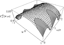
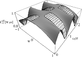
Figure 1: The Holevo bound for the state parameter (a) $\theta_{0}=0.2,\vec{\theta}=0.346(1,1)/\sqrt{2}$ and (b) $\theta_{0}=0.275,\vec{\theta}=0.476(1,1)/\sqrt{2}$ as a function of the wight-matrix parameter $(w,\omega)$ given in Eq. (113). The gray areas indicate the case for $C^{H}_{\theta}[W]=C^{R}_{\theta}[W]+S_{\theta}[W]$, whereas the white-meshed region indicate the case for $C^{H}_{\theta}[W]=C^{R}_{\theta}[W]$.

From these figures, we see that the Holevo bound coincides with the RLD CR bound for relatively large choice of the weight matrix in Fig. 1, where as the opposite observation holds for Fig. 1. To gain a deeper insight, let us calculate the value of quantities $\gamma_{\theta,i}:=\langle{\bm{s}}_{\theta}|{\bm{\ell}}_{\theta,i}\rangle$ ($i=1,2$). Then, we get $\gamma_{\theta,1}=\gamma_{\theta,2}=0.292$ for the case (a) and $\gamma_{\theta,1}=\gamma_{\theta,2}=0.483$ for the case (b). Since vanishing of these quantities is equivalent to the D-invariance of a model (Lemma III.3), we naively expect that the smaller values of them imply that a model behaves more D-invariant-like. Indeed, the examples presented here agree with our intuition, yet more detail analysis is needed to make any conclusion.

V.4 Transition in the parameter space

We briefly discuss another important observation of this paper. A generic model, other than special cases discussed before, exhibits a transition in the structure of the Holevo bound for a fixed weight matrix when we change the estimation parameter $\theta$. A rough sketch of this argument is that a change in the weight matrix is amount to that in the parameter and vice versa. This is a well-known fact in the pointwise estimation setting nagaoka91 ; FN99 . Below we briefly show such an example. The model is same as the generic model (106) analyzed the previous subsection.

As noted before, a change in the weight-matrix parameter $\omega_{0}\to\omega_{0}+\omega$ is equivalent to rotate the parameter $(\theta^{1},\theta^{2})$ by the angle $\omega$. Depending upon the choice of the weight matrix, we can also observe a similar transition when we change the parameter $\theta$ in the set $\Theta$. We set the weight matrix to be a diagonal matrix $W_{0}=\mathrm{diag}(0.55,0.45)$ and $\theta_{0}=0.35$. Figure 2 plots the Holevo bound as a function of the state parameter $\theta=(\theta^{1},\theta^{2})$. The gray area indicates the region where $C^{H}_{\theta}[W_{0}]=C^{R}_{\theta}[W_{0}]+S_{\theta}[W_{0}]$ holds, whereas the white-meshed region indicates the case for $C^{H}_{\theta}[W_{0}]=C^{R}_{\theta}[W_{0}]$. This shows that the Holevo bound coincides with the RLD CR bound for a certain subset of the parameter space.

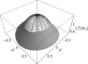
Figure 2: The Holevo bound for the weight matrix $W_{0}=\mathrm{diag}(0.55,0.45)$ and $\theta_{0}=0.35$ as a function of the state parameter $\vec{\theta}=(\theta^{1},\theta^{2})$. The gray area indicates the case for $C^{H}_{\theta}[W]=C^{R}_{\theta}[W]+S_{\theta}[W]$, whereas the white-meshed region indicates the case for $C^{H}_{\theta}[W]=C^{R}_{\theta}[W]$.

VI Concluding remarks

In this paper, we have derived a closed formula for the fundamental precision bound, the Holevo bound, for any two-parameter qubit estimation problem in the pointwise estimation setting. This bound is known to be asymptotically achievable by the optimal sequence of estimators consisting of jointly performed measurements under some regularity conditions. Since there exist explicit formulas for the Holevo bound for the pure-state qubit model, qubit mixed-state models with one and three parameters, our result completes a list of the fundamental precision bounds in terms of quantum versions of Fisher information, which is calculated from a given quantum parametric model, as far as qubit models are concerned. The obtained formula shows several new insights into the property of the Holevo bound for quantum parameter estimation problems. In the following we shall list concluding remarks together with outlook for future works.

First, the necessary and sufficient conditions for the asymptotic achievability of the SLD and RLD CR bounds are derived when estimating any two-parameter family of qubit states. In particular, the notation of asymptotically classical models is proposed, in which all SLD operators commute with each other on the trace of a given parametric state. In this case, the weight matrix can be eliminated and the problem becomes similar to the classical statistics in the asymptotic limit, where the SLD Fisher information plays the same role as the Fisher information. We note that the notion of asymptotic classicality can be extended to any models on any finite-dimensional system and the same statement obtained for the qubit case holds: The Holevo bound coincides with the SLD CR bound if and only if the model is asymptotically classical. The detail of this result shall be given in the subsequent paper.

Second, the RLD CR bound is shown to be achieved for a certain choice of the weight matrix even though the model is not D-invariant. This result emphasizes the importance of the RLD Fisher information for general qubit parameter estimation problems. Since the imaginary parts of the inverse of the RLD Fisher information matrix and the $Z_{\theta}$ matrix are always identical for two-parameter qubit mixed-state models, we cannot immediately conclude that this is the general statement or not. It might well be that the only real part of the inverse of RLD Fisher information matrix plays an important role in higher dimensional systems. This deserves further studies and shall be analyzed as an extension of the present work.

Third, our result also provides the (unique) minimizer to the optimization problem appearing in the definition of the Holevo bound. This set of observables, which are locally unbiased in the sense of Eq. (16), can be used to construct an optimal sequence of POVMs that attains the Holevo bound asymptotically. This line of approach has been proposed by Hayashi, who reported a theorem without proof to realize the construction of POVMs on the tensor product states hayashi03 . His approach is different from other approaches given in Refs. HM08 ; GK06 ; YFG13 and it may need more refined arguments to complete his theorem.

Last, smooth transitions in the structure of the Holevo bound is shown to occur in general. Since this happens in the simplest quantum system, we expect similar phenomena occur in higher dimensional systems as well. However, we do not know whether or not the number of different forms is always two as demonstrated here. The techniques used in this paper can be applied to two-parameter estimation problems in higher dimensional systems, and we shall make progress in due course.

Appendix A Proofs for lemmas

A.1 Leema III.1

Proof follows from a straightforward calculation. We substitute ${\bm{x}}^{i}={\bm{\ell}}_{\theta}^{i}+\xi^{i}{\bm{\ell}}_{\theta}^{\bot}$ into the second line of Eqs. (64). The first term reads

$$\langle{\bm{x}}^{i}|Q_{\theta}^{-1}{\bm{x}}^{j}\rangle =\langle{\bm{\ell}}_{\theta}^{i}|Q_{\theta}^{-1}{\bm{\ell}}_{\theta}^{j}\rangle+\xi^{i}\xi^{j}\langle{\bm{\ell}}_{\theta}^{\bot}|{Q}_{\theta}^{-1}{\bm{\ell}}_{\theta}^{\bot}\rangle$$

$$=g_{\theta}^{ij}+\xi^{i}\xi^{j}\langle{\bm{\ell}}_{\theta}^{\bot}|{Q}_{\theta}^{-1}{\bm{\ell}}_{\theta}^{\bot}\rangle,$$ (114)

where the relation $\langle{\bm{\ell}}_{\theta}^{i}|Q_{\theta}^{-1}{\bm{\ell}}_{\theta}^{\bot}\rangle=0$ for $i=1,2$ and Eq. (51) are used. Note $\langle{\bm{a}}|F_{\theta}{\bm{a}}\rangle=0$ for all ${\bm{a}}\in{\mathbb{R}}^{2}$, then the second term is calculated as

$$\sum_{i,j=1}^{2}|\langle{\bm{x}}^{i}|F_{\theta}{\bm{x}}^{j}\rangle| =2|\langle{\bm{x}}^{1}|F_{\theta}{\bm{x}}^{2}\rangle|$$ (115)

$$=2|\langle{\bm{\ell}}_{\theta}^{1}|F_{\theta}{\bm{\ell}}_{\theta}^{2}\rangle +\xi^{1}\langle{\bm{\ell}}_{\theta}^{\bot}|F_{\theta}{\bm{\ell}}_{\theta}^{2}\rangle+\xi^{2}\langle{\bm{\ell}}_{\theta}^{1}|F_{\theta}{\bm{\ell}}_{\theta}^{\bot}\rangle|$$

$$=2|\langle{\bm{\ell}}_{\theta}^{1}|F_{\theta}{\bm{\ell}}_{\theta}^{2}\rangle +\xi^{1}(1-s_{\theta}^{2})\gamma_{\theta,1}+\xi^{2}(1-s_{\theta}^{2})\gamma_{\theta,2}|,$$

where $\langle{\bm{\ell}}_{\theta}^{\bot}|F_{\theta}{\bm{\ell}}_{\theta}^{2}\rangle=(1-s_{\theta}^{2})\gamma_{\theta,1}$ and $\langle{\bm{\ell}}_{\theta}^{\bot}|F_{\theta}{\bm{\ell}}_{\theta}^{1}\rangle=-(1-s_{\theta}^{2})\gamma_{\theta,2}$ are used. Combining the above expressions, we get the expression of this lemma. $\square$

A.2 Lemma III.2

1. $\langle{\bm{\ell}}_{\theta}^{\bot}|{Q}_{\theta}^{-1}{\bm{\ell}}_{\theta}^{\bot}\rangle=(1-s_{\theta}^{2})\det\,G_{\theta}=(1-s_{\theta}^{2})^{2}\det\tilde{G}_{\theta}$:
For convenience, let us define

$${\bm{n}}_{\theta} :=\partial_{1}{\bm{s}}_{\theta}\times\partial_{2}{\bm{s}}_{\theta},$$ (116)

$${\bm{m}}_{\theta} :={\bm{\ell}}_{\theta,1}\times{\bm{\ell}}_{\theta,2},$$

which are related by ${\bm{n}}_{\theta}=(1-s_{\theta}^{2})Q_{\theta}{\bm{m}}_{\theta}$. The standard vector analysis shows

$$\langle{\bm{m}}_{\theta}|{\bm{m}}_{\theta}\rangle =\langle{\bm{\ell}}_{\theta,1}|{\bm{\ell}}_{\theta,1}\rangle\langle{\bm{\ell}}_{\theta,2}|{\bm{\ell}}_{\theta,2}\rangle-(\langle{\bm{\ell}}_{\theta,1}|{\bm{\ell}}_{\theta,2}\rangle)^{2},$$

$${\bm{s}}_{\theta}\times{\bm{m}}_{\theta} =\gamma_{\theta,2}{\bm{\ell}}_{\theta,1}-\gamma_{\theta,1}{\bm{\ell}}_{\theta,2}.$$

From the expression (48), the components of the SLD Fisher information matrix is expressed as $g_{\theta,ij}=\langle{\bm{\ell}}_{\theta,i}|{\bm{\ell}}_{\theta,j}\rangle-\gamma_{\theta,i}\gamma_{\theta,j}$. Then, the determinant of the SLD Fisher information matrix is calculated as

$$\det\,G_{\theta} =(\langle{\bm{\ell}}_{\theta,1}|{\bm{\ell}}_{\theta,1}\rangle-\gamma_{\theta,1}^{2})(\langle{\bm{\ell}}_{\theta,2}|{\bm{\ell}}_{\theta,2}\rangle-\gamma_{\theta,2}^{2})$$

$$\quad-(\langle{\bm{\ell}}_{\theta,1}|{\bm{\ell}}_{\theta,2}\rangle-\gamma_{\theta,1}\gamma_{\theta,2})^{2}$$

$$=\langle{\bm{\ell}}_{\theta,1}|{\bm{\ell}}_{\theta,1}\rangle\langle{\bm{\ell}}_{\theta,2}|{\bm{\ell}}_{\theta,2}\rangle-(\langle{\bm{\ell}}_{\theta,1}|{\bm{\ell}}_{\theta,2}\rangle)^{2}$$

$$\quad-|\gamma_{\theta,2}{\bm{\ell}}_{\theta,1}-\gamma_{\theta,1}{\bm{\ell}}_{\theta,2}|^{2}$$

$$=\langle{\bm{m}}_{\theta}|{\bm{m}}_{\theta}\rangle-\langle{\bm{s}}_{\theta}\times{\bm{m}}_{\theta}|{\bm{s}}_{\theta}\times{\bm{m}}_{\theta}\rangle$$

$$=(1-s_{\theta}^{2})\langle{\bm{m}}_{\theta}|Q_{\theta}{\bm{m}}_{\theta}\rangle$$

$$=\frac{1}{1-s_{\theta}^{2}}\langle{\bm{n}}_{\theta}|{Q}_{\theta}^{-1}{\bm{n}}_{\theta}\rangle,$$

and hence we obtain $\langle{\bm{\ell}}_{\theta}^{\bot}|{Q}_{\theta}^{-1}{\bm{\ell}}_{\theta}^{\bot}\rangle=(1-s_{\theta}^{2})\det\,G_{\theta}$.

Next, we use the relation for the RLD Fisher information; $\tilde{g}_{\theta,ij}=(1-s_{\theta}^{2})^{-1}[\langle{\bm{\ell}}_{\theta,i}|{\bm{\ell}}_{\theta,j}\rangle-(2-s_{\theta}^{2})\gamma_{\theta,i}\gamma_{\theta,j}-\mathrm{i}\langle{\bm{\ell}}_{\theta,i}|F_{\theta}{\bm{\ell}}_{\theta,j}\rangle]$ to calculate the determinant $\det\,\tilde{G}_{\theta}$ as

$$(1-s_{\theta}^{2})^{2}\det\,\tilde{G}_{\theta}$$

$$=(\langle{\bm{\ell}}_{\theta,1}|{\bm{\ell}}_{\theta,1}\rangle-(2-s_{\theta}^{2})\gamma_{\theta,1}^{2})(\langle{\bm{\ell}}_{\theta,2}|{\bm{\ell}}_{\theta,2}\rangle-(2-s_{\theta}^{2})\gamma_{\theta,2}^{2})$$

$$\quad-|\langle{\bm{\ell}}_{\theta,1}|{\bm{\ell}}_{\theta,2}\rangle-(2-s_{\theta}^{2})\gamma_{\theta,1}\gamma_{\theta,2}-\mathrm{i}\langle{\bm{\ell}}_{\theta,1}|F_{\theta}{\bm{\ell}}_{\theta,2}\rangle|^{2}$$

$$=\langle{\bm{m}}_{\theta}|{\bm{m}}_{\theta}\rangle-(2-s_{\theta}^{2})\langle{\bm{s}}_{\theta}\times{\bm{m}}_{\theta}|{\bm{s}}_{\theta}\times{\bm{m}}_{\theta}\rangle-|\langle{\bm{s}}_{\theta}|{\bm{m}}_{\theta}\rangle|^{2}$$

$$=(1-s_{\theta}^{2})^{2}\langle{\bm{m}}_{\theta}|Q_{\theta}{\bm{m}}_{\theta}\rangle.$$

This proves the relation; $(1-s_{\theta}^{2})\det\,\tilde{G}_{\theta}=\det\,G_{\theta}$. $\square$

2. $2\sqrt{\det W}\left|\langle{\bm{\ell}}_{\theta}^{1}|F_{\theta}{\bm{\ell}}_{\theta}^{2}\rangle\right|=\mathrm{TrAbs}\{W\mathrm{Im}\,\tilde{G}_{\theta}^{-1}\}=\mathrm{TrAbs}\{W\mathrm{Im}\,Z_{\theta}\}$:
From the definition for the matrix $Z_{\theta}$, the imaginary part is expressed as

$$\mathrm{Im}\,Z_{\theta}=\langle{\bm{\ell}}_{\theta}^{1}|F_{\theta}{\bm{\ell}}_{\theta}^{2}\rangle\left(\begin{array}[]{cc}0&1\\ -1&0\end{array}\right),$$ (117)

and the straightforward calculation yields

$$\mathrm{TrAbs}\left\{W\mathrm{Im}\,Z_{\theta}\right\}=2\sqrt{\det W}\left|\langle{\bm{\ell}}_{\theta}^{1}|F_{\theta}{\bm{\ell}}_{\theta}^{2}\rangle\right|.$$ (118)

The imaginary part of the RLD Fisher information matrix is

$$\mathrm{Im}\,\tilde{G}_{\theta}=\frac{\langle{\bm{\ell}}_{\theta,1}|F_{\theta}{\bm{\ell}}_{\theta,2}\rangle}{1-s_{\theta}^{2}}\left(\begin{array}[]{cc}0&-1\\ 1&0\end{array}\right),$$ (119)

and the imaginary part of the inverse is

$$\mathrm{Im}\,\{\tilde{G}_{\theta}^{-1}\}=\frac{\langle{\bm{\ell}}_{\theta,1}|F_{\theta}{\bm{\ell}}_{\theta,2}\rangle}{\det{G}_{\theta}}\left(\begin{array}[]{cc}0&1\\ -1&0\end{array}\right),$$ (120)

where we use $(1-s_{\theta}^{2})\det\,\tilde{G}_{\theta}=\det\,G_{\theta}$. It is easy to show $\langle{\bm{\ell}}_{\theta}^{1}|F_{\theta}{\bm{\ell}}_{\theta}^{2}\rangle=\langle{\bm{\ell}}_{\theta,1}|F_{\theta}{\bm{\ell}}_{\theta,2}\rangle/\det G_{\theta}$ and thus we obtain the important relationship; $\mathrm{Im}\,Z_{\theta}=\mathrm{Im}\,\tilde{G}_{\theta}^{-1}$. This proves the claim. $\square$

3. $(\vec{\gamma}_{\theta}|W^{-1}\vec{\gamma}_{\theta})={\det W^{-1}G_{\theta}}\left(C_{\theta}^{Z}[W]-C_{\theta}^{R}[W]\right)/{(1-s_{\theta}^{2})}$:
This can be shown by the following calculations:

$$\det W\times(\vec{\gamma}_{\theta}|W^{-1}\vec{\gamma}_{\theta})$$

$$=w_{22}\gamma_{\theta,1}^{2}+w_{11}\gamma_{\theta,2}^{2}-2w_{12}\gamma_{\theta,1}\gamma_{\theta,2}$$

$$=(1-s_{\theta}^{2})^{-1}(w_{22}g_{\theta,11}+w_{11}g_{\theta,22}-2w_{12}g_{12})$$

$$\quad-\mathrm{Re}\,(w_{22}\tilde{g}_{\theta,11}+w_{11}\tilde{g}_{\theta,22}-2w_{12}\tilde{g}_{12})$$

$$=(1-s_{\theta}^{2})^{-1}\det G_{\theta}\mathrm{Tr}\left\{WG_{\theta}^{-1}\right\}-\det\tilde{G}_{\theta}\mathrm{Tr}\left\{W\mathrm{Re}\,\tilde{G}_{\theta}^{-1}\right\}$$

$$=\frac{\det G_{\theta}}{1-s_{\theta}^{2}}\mathrm{Tr}\left\{W(G_{\theta}^{-1}-\mathrm{Re}\,\tilde{G}_{\theta}^{-1})\right\}$$

$$=\frac{\det G_{\theta}}{1-s_{\theta}^{2}}\left(C_{\theta}^{Z}[W]-C_{\theta}^{R}[W]\right).\ \square$$

A.3 Lemma III.3

Since the imaginary parts of the inverse of the RLD Fisher information matrix and the matrix $Z_{\theta}$ are always identical for two-parameter qubit models, equivalence between 1 and 2 is the direct consequence of Lemma B.1. We next note the following relation:

$$G_{\theta}^{-1}-\mathrm{Re}\,\tilde{G}_{\theta}^{-1}=\frac{1}{\det\tilde{G}_{\theta}}\left(\begin{array}[]{cc}\gamma_{\theta,2}^{2}&-\gamma_{\theta,1}\gamma_{\theta,2}\\ -\gamma_{\theta,1}\gamma_{\theta,2}&\gamma_{\theta,1}^{2}\end{array}\right),$$

which follows from Eq. (61) and Lemma III.2-1. Thus $G_{\theta}^{-1}-\mathrm{Re}\,\tilde{G}_{\theta}^{-1}=0$ if and only if $\gamma_{\theta,1}=\gamma_{\theta,2}=0$.

To show the statement about global D-invariance, we only need to show $\gamma_{\theta,1}=\gamma_{\theta,2}=0$ for all $\theta\in\Theta$ if and only if $s_{\theta}=|{\bm{s}}_{\theta}|$ is independent of $\theta$. When $\gamma_{\theta,i}=\langle{\bm{s}}_{\theta}|{\bm{\ell}}_{\theta,i}\rangle=0$ $\Leftrightarrow$ $\langle{\bm{s}}_{\theta}|\partial_{i}{\bm{s}}_{\theta}\rangle=(1/2)\partial_{i}|{\bm{s}}_{\theta}|^{2}=0$ holds, the integration of this condition gives $|{\bm{s}}_{\theta}|$ is independent of $\theta=(\theta^{1},\theta^{2})$. Conversely, $|{\bm{s}}_{\theta}|$ does not depend on $\theta$, we obtain $\gamma_{\theta,i}=0$ ($i=1,2$) for all $\theta\in\Theta$. $\square$

A.4 Lemma III.4

When $\vec{b}=\vec{0}$, the function to be minimized is $f(\vec{\xi})=(\vec{\xi}|A\vec{\xi})+2|c|$. Since $A$ is positive-definite, the minimum is $2|c|$ and is attained by $\vec{\xi}_{*}=\vec{0}$.

For the other case ($\vec{b}\neq\vec{0}$), introducing the new variables through

$$\vec{\eta}=BA^{1/2}\vec{\xi},\ \mathrm{with}\ B=\left(\begin{array}[]{c}\vec{b}^{T}A^{-1/2}\\ \vec{b}^{T}A^{-1/2}\left(\begin{array}[]{cc}0&-1\\ 1&0\end{array}\right)\end{array}\right),$$

we can express the function $f(\vec{\xi})$ as

$$f(\vec{\eta})=\frac{1}{\alpha}(\eta_{1}^{2}+\eta_{2}^{2})+2|\eta_{1}+c|,$$ (121)

where $\alpha=(\vec{b}|A^{-1}\vec{b})$ is a positive constant. The minimum of this simple quadratic function is obtained by analyzing the case $\eta_{1}+c>0$ and $\eta_{1}+c\leq 0$ separately. The result is

$$\min_{\vec{\eta}\in{\mathbb{R}}^{2}}f(\vec{\eta})=\begin{cases}-\alpha+2c\quad\mathrm{if}c\geq\alpha\\ \displaystyle\frac{c^{2}}{\alpha}\qquad\qquad\mathrm{if}|c|<\alpha\\ -\alpha-2c\quad\mathrm{if}c\leq-\alpha\end{cases},$$ (122)

and the unique minimizer $\vec{\eta_{*}}=(\zeta_{*},0)^{T}$ is

$$\zeta_{*}=\begin{cases}-\alpha\quad\mathrm{if}c\geq\alpha\\ -c\quad\quad\mathrm{if}|c|<\alpha\\ \alpha\qquad\mathrm{if}c\leq-\alpha\end{cases}.$$ (123)

This solution can be translated into the original variables $\vec{\xi}$ to prove the lemma. $\square$

Appendix B Supplemental materials

B.1 Canonical projection and invariant subspace

In this appendix, we summarize the concept of canonical projection and invariant subspace for an inner product space on real numbers. These results can be generalized to more general settings to be applied to the quantum estimation problem.

Consider an $n$-dimensional vector space $V$ on ${\mathbb{R}}$ and an inner product on it $\langle\cdot,\cdot\rangle:V^{2}\to{\mathbb{R}}$. Let $w_{1},w_{2},\dots,w_{k}\in V$ ($k<n$) be a set of linearly independent vectors and define the subspace $W=\mathrm{span}_{\mathbb{R}}\{w_{1},w_{2},\dots,w_{k}\}\subset V$ spanned by these vectors. We define a real positive semi-definite matrix $G=[\langle w_{i},w_{j}\rangle]_{i,j\in\{1,2,\dots,k\}}$ and its inverse by $G^{-1}=[g^{ij}]_{i,j}$. A set of vectors $\{w^{i}=\sum_{j}g^{ji}w_{j}\}_{i=1}^{k}$ forms the dual basis of $\{w_{i}\}_{i=1}^{k}$.

Given a vector $v\in V$, the canonical projection of $v$ onto the subspace $W$ is a map $\pi_{W}:\ V\to W$ such that

$$\pi_{W}(v)=\sum_{i=1}^{k}\langle v,w^{i}\rangle w_{i}\in W.$$ (124)

This canonical projection is unique and it preserves the inner product as

$$\langle\pi_{W}(v),w\rangle=\langle v,w\rangle\ \forall w\in W,\ \forall v\in V.$$ (125)

Consider any element $v\in V$ and the condition $v\in W$ is equivalently expressed as follows.

$$v\in W \Leftrightarrow\pi_{W}(v)=v$$

$$\Leftrightarrow\forall v^{\prime}\in W^{\bot}\ \langle v^{\prime},v\rangle=0$$

$$\Leftrightarrow\forall v^{\prime}\in V\ \langle v^{\prime}-\pi_{W}(v^{\prime}),v\rangle=0$$

$$\Leftrightarrow\forall(v^{1},v^{2},\dots,v^{k})\in V^{k},$$

$$\quad\forall i(\pi_{W}(v^{i})=w^{i}\Rightarrow\langle v^{i}-w^{i},v\rangle=0),$$

where $W^{\bot}=\{v\in V\,|\,\langle v,w\rangle=0\forall w\in W\}$ is the (unique) orthogonal complement of $W$.

Next, consider a linear map $A$ from $V$ to itself. The subspace is said invariant under the map $A$, if the image of $W$ is a subset of $W$, i.e., $A(w)\in W$ holds for $\forall w\in W$. Using the above equivalence, this can be written as

$$W\mbox{ is an}\mbox{ invariant subspace under $A$}$$ (126)

$$\Leftrightarrow\forall i\ A(w_{i})\in W$$

$$\Leftrightarrow\forall i\forall v^{\prime}\in W^{\bot}\ \langle v^{\prime},A(w_{i})\rangle=0$$

$$\Leftrightarrow\forall(v^{1},v^{2},\dots,v^{k})\in V^{k},$$

$$\quad\forall i,j(\pi_{W}(v^{i})=w^{i}\Rightarrow\langle v^{i}-w^{i},A(w_{j})\rangle=0).$$

B.2 Characterization of D-invariant model

Lemma B.1

Let $L_{\theta}^{i}$ ($\tilde{L}_{\theta}^{i}$) be the SLD (RLD) dual operator and $G_{\theta}$ ($\tilde{G}_{\theta}$) be the SLD (RLD) Fisher information matrix, respectively. Define a $k\times k$ hermite matrix by $Z_{\theta}=[\langle L_{\theta}^{i},L_{\theta}^{j}\rangle_{\rho_{\theta}}^{+}]_{i,j\in\{1,\dots,k\}}$, then, the following conditions are equivalent.

1. ${\cal M}$ is D-invariant at $\theta$.

2. ${\cal D}_{\theta}(L_{\theta}^{i})=\sum_{j}(\mathrm{Im}\,Z_{\theta})^{ji}L_{\theta,j}$, $\forall i\in\{1,2,\dots,k\}$.

3. $Z_{\theta}=\tilde{G}_{\theta}^{-1}$

4. $L_{\theta}^{i}=\tilde{L}_{\theta}^{i}$, $\forall i\in\{1,2,\dots,k\}$.

5. $\forall X^{i}\in{\cal L}_{h}({\cal H})$, $X^{i}-L_{\theta}^{i}\bot T_{\theta}({\cal M})$ with respect to $\langle\cdot,\cdot\rangle_{\rho_{\theta}}$ $\Rightarrow$ $X^{i}-L_{\theta}^{i}\bot T_{\theta}({\cal M})$ with respect to $\langle\cdot,\cdot\rangle_{\rho_{\theta}}^{+}$.

In the above lemma, $\langle X,Y\rangle_{\rho_{\theta}}:=\mathrm{Re}\,\mathrm{tr}\left(\rho_{\theta}YX^{*}\right)$ and $\langle X,Y\rangle_{\rho_{\theta}}^{+}:=\mathrm{tr}\left(\rho_{\theta}YX^{*}\right)$ denote the SLD and RLD inner products, respectively.

• We prove this lemma by the chain; $1\Rightarrow 2\Rightarrow 3\Rightarrow 4\Rightarrow 5\Rightarrow 1$. Suppose that a given model is D-invariant, this is equivalent to say that the action of the commutation operator on the SLD dual operators is expressed as

  $${\cal D}_{\theta}(L_{\theta}^{i})=\sum_{j}c^{ji}L_{\theta,j},$$ (127)

  with some real coefficients $c^{ij}$. These coefficients are expressed as

  $$c^{ji}=\langle L_{\theta}^{i},{\cal D}_{\theta}(L_{\theta}^{j})\rangle_{\rho_{\theta}},$$ (128)

  which directly from the orthogonality condition (13). Using the relation (36), the right hand side is also expressed as $\mathrm{Im}\,z_{\theta}^{ij}$, and if the model is D-invariant at $\theta$,

  $${\cal D}_{\theta}(L_{\theta}^{i})=\sum_{j}(\mathrm{Im}\,Z_{\theta})^{ji}L_{\theta,j}.$$ (129)

  Hence we show $1\Rightarrow 2$.

  Next, if the condition (129) holds, the SLD inner product between ${\cal D}_{\theta}(L_{\theta}^{i})$ and the RLD dual operator $\tilde{L}_{\theta}^{j}$ gives

  $$\langle\tilde{L}_{\theta}^{i},{\cal D}_{\theta}(L_{\theta}^{j})\rangle_{\rho_{\theta}}=\sum_{k}c^{kj}\langle\tilde{L}_{\theta}^{i},L_{\theta}^{k}\rangle_{\rho_{\theta}}=c^{ji}.$$ (130)

  The left hand side is also calculated from Eq. (37) as $-\mathrm{i}(\tilde{g}_{\theta}^{ij}-g_{\theta}^{ij})$. Therefore, we show

  $$c^{ji}=\mathrm{Im}\,z_{\theta}^{ij}=-\mathrm{i}(\tilde{g}_{\theta}^{ij}-g_{\theta}^{ij})\ \Leftrightarrow\ \tilde{G}_{\theta}^{-1}=Z_{\theta},$$ (131)

  holds, if the condition (129) holds, that is, $2\Rightarrow 3$.

  Consider an arbitrary linear operator $X$ and assume the condition (131). In this case, the RLD inner product between $X$ and $\tilde{L}_{\theta}^{i}$ is calculated as

  $$\langle X,\tilde{L}_{\theta}^{i}\rangle_{\rho_{\theta}}^{+} =\sum_{k}\tilde{g}_{\theta}^{kj}\langle X,\tilde{L}_{\theta,k}\rangle_{\rho_{\theta}}^{+}$$

  $$=\sum_{k}z_{\theta}^{kj}\langle X,\tilde{L}_{\theta,k}\rangle_{\rho_{\theta}}^{+}$$

  $$=\sum_{k}z_{\theta}^{kj}\langle X,L_{\theta,k}\rangle_{\rho_{\theta}}$$

  $$=\sum_{k}(g_{\theta}^{kj}\langle X,L_{\theta,k}\rangle_{\rho_{\theta}}+\mathrm{i}\mathrm{Im}\,z^{kj}\langle X,L_{\theta,k}\rangle_{\rho_{\theta}})$$

  $$=\langle X,L_{\theta}^{j}\rangle_{\rho_{\theta}}+\mathrm{i}\langle X,{\cal D}_{\theta}(L_{\theta}^{j})\rangle_{\rho_{\theta}}$$

  $$=\langle X,L_{\theta}^{j}\rangle_{\rho_{\theta}}^{+},$$

  where Eq. (131), and the several equations presented in Sec. II.3.2 are used. Since $X\in{\cal L}({\cal H})$ is arbitrary, it implies

  $$L_{\theta}^{i}=\tilde{L}_{\theta}^{i}\mbox{ folds for all }i\in\{1,2,\dots,k\}.$$ (132)

  Therefore, we show $3\Rightarrow 4$.

  Next, let us assume the condition (132) and we show that this implies the condition $5$, that is, $\forall X^{i}\in{\cal L}_{h}({\cal H})$, $X^{i}-L_{\theta}^{i}\bot T_{\theta}({\cal M})$ with respect to $\langle\cdot,\cdot\rangle_{\rho_{\theta}}$ $\Rightarrow$ $X^{i}-L_{\theta}^{i}\bot T_{\theta}({\cal M})$ with respect to $\langle\cdot,\cdot\rangle_{\rho_{\theta}}^{+}$. This is because

  $$X^{i}- L_{\theta}^{i}\bot T_{\theta}({\cal M})\mathrm{w.r.t.}\langle\cdot,\cdot\rangle_{\rho_{\theta}}$$

  $$\Leftrightarrow\forall j\langle X^{i}-L_{\theta}^{i},L_{\theta,j}\rangle_{\rho_{\theta}}$$

  $$\Leftrightarrow\forall j\langle X^{i}-L_{\theta}^{i},\tilde{L}_{\theta,j}\rangle_{\rho_{\theta}}^{+}$$

  $$\Rightarrow\forall j\langle X^{i}-L_{\theta}^{i},\tilde{L}_{\theta}^{j}\rangle_{\rho_{\theta}}^{+}$$

  $$\Leftrightarrow\forall j\langle X^{i}-L_{\theta}^{i},L_{\theta}^{j}\rangle_{\rho_{\theta}}^{+}$$

  $$\Leftrightarrow X^{i}-L_{\theta}^{i}\bot T_{\theta}({\cal M})\mathrm{w.r.t.}\langle\cdot,\cdot\rangle_{\rho_{\theta}}^{+}.$$

  The remaining to be shown is that the condition,

  $$\forall X^{i}\in{\cal L}_{h}({\cal H}),\ \forall i(X^{i}-L_{\theta}^{i}\bot T_{\theta}({\cal M})\mbox{ w.r.t. }\langle\cdot,\cdot\rangle_{\rho_{\theta}}\\ \Rightarrow\ X^{i}-L_{\theta}^{i}\bot T_{\theta}({\cal M})\mbox{ w.r.t. }\langle\cdot,\cdot\rangle_{\rho_{\theta}}^{+}),$$ (133)

  implies the D-invariance of the model. Consider a set of hermite operators $\vec{X}=(X^{1},X^{2},\dots,X^{k})$ and suppose the above condition (133). Since $X^{i}-L_{\theta}^{i}\bot T_{\theta}({\cal M})\mbox{ w.r.t. }\langle\cdot,\cdot\rangle_{\rho_{\theta}}$ is equivalent to $\pi_{T_{\theta}}(X^{i})=L_{\theta}^{i}$ with $\pi_{T_{\theta}}$ the canonical projection on $T_{\theta}({\cal M})$, we can rewrite it as

  $$\forall X^{i}\in{\cal L}_{h}({\cal H}),\ \forall i,j(\langle X^{i}-L_{\theta}^{i},L_{\theta,j}\rangle_{\rho_{\theta}}\ \Rightarrow\ \langle X^{i}-L_{\theta}^{i},L_{\theta,j}\rangle_{\rho_{\theta}}^{+}).$$ (134)

  The use of Eq. (35) leads $\langle X^{i}-L_{\theta}^{i},L_{\theta,j}\rangle_{\rho_{\theta}}\Rightarrow\langle X^{i}-L_{\theta}^{i},L_{\theta,j}\rangle_{\rho_{\theta}}^{+}$ $\Rightarrow$ $\langle X^{i}-L_{\theta}^{i},L_{\theta,j}\rangle_{\rho_{\theta}}\Rightarrow\langle X^{i}-L_{\theta}^{i},{\cal D}_{\theta}(L_{\theta,j})\rangle_{\rho_{\theta}}$. Then, the equivalent condition (126) can be applied to conclude that the subspace $T_{\theta}({\cal M})$ is invariant under the action of linear operator ${\cal D}_{\theta}$, that is, the model is D-invariant. $\square$

B.3 Proof for Theorem II.5

i) Proof for the RLD CR bound case:
The sufficiency (D-invariant model $\Rightarrow C_{\theta}^{H}[W]=C_{\theta}^{R}[W]$ for all $W>0$.) follows from Proposition II.4. If the Holevo bound is identical to the RLD CR bound for all weight matrices, then all the RLD dual operators must be hermite, i.e., $(\tilde{L}_{\theta}^{i})^{*}=\tilde{L}_{\theta}^{i}$ for all $i=1,2,\dots,k$. To see this, we note that $\vec{X}=(X^{1},X^{2},\dots,X^{k})\in{\cal X}_{\theta}$ implies $\vec{X}\in\tilde{{\cal X}}_{\theta}:=\{\vec{X}\,|\,\forall i\,X^{i}\in{\cal L}({\cal H}),\mathrm{tr}\left(\rho_{\theta}X^{i}\right)=0,\ \forall i,j\,\mathrm{tr}\left(\partial_{i}\rho_{\theta}X^{j}\right)=\delta^{j}_{\,i}\}$. By rewriting $\mathrm{tr}\left(\partial_{i}\rho_{\theta}X^{j}\right)=\delta^{j}_{\,i}\Leftrightarrow\langle X^{i}-\tilde{L}_{\theta}^{i},\tilde{L}_{\theta,j}\rangle_{\rho_{\theta}}^{+}=0$, we see that $X^{i}-\tilde{L}_{\theta}^{i}$ ($i=1,2,\dots,k$) are orthogonal to the complex span of the RLD operators, $\tilde{T}_{\theta}({\cal M}):=\mathrm{span}_{\mathbb{C}}\{\tilde{L}_{\theta,i}\}$. It is straightforward to show that $Z_{\theta}[\vec{X}]=Z_{\theta}[\vec{X}-\vec{\tilde{L}}_{\theta}]+Z_{\theta}[\vec{\tilde{L}}_{\theta}]$ holds for $\vec{X}\in\tilde{{\cal X}}_{\theta}$, where $\vec{\tilde{L}}_{\theta}=(\tilde{L}_{\theta}^{1},\tilde{L}_{\theta}^{2},\dots,\tilde{L}_{\theta}^{k})$ is the collection of the RLD dual operators. Since the matrix $Z_{\theta}[\vec{X}-\vec{\tilde{L}}_{\theta}]$ is positive semi-definite, and hence, we obtain

$$\vec{X}\in\tilde{{\cal X}}_{\theta}\Rightarrow Z_{\theta}[\vec{X}]\geq\tilde{G}_{\theta}^{-1},$$ (135)

and the equality if and only if $\forall i\,X^{i}=\tilde{L}_{\theta}^{i}$ holds. Thus, all $\tilde{L}_{\theta}^{i}$ need to be in the set ${\cal X}_{\theta}$.

Next, we use the relation between the SLD and RLD operators, $(I+\mathrm{i}{\cal D}_{\theta})(\tilde{L}_{\theta,i})=L_{\theta,i}$ (see Eq. (35)), to get

$$(I+\mathrm{i}{\cal D}_{\theta})(\tilde{L}_{\theta}^{i})=\sum_{j}\tilde{g}^{ji}L_{\theta,j}.$$ (136)

Then, the conditions $(\tilde{L}_{\theta}^{i})^{*}=\tilde{L}_{\theta}^{i}$ for all $i$ imply

$$\tilde{L}_{\theta}^{i} =\sum_{j}\mathrm{Re}\,\{\tilde{g}^{ji}\}L_{\theta,j},$$ (137)

$${\cal D}_{\theta}(\tilde{L}_{\theta}^{i}) =\sum_{j}\mathrm{Im}\,\{\tilde{g}^{ji}\}L_{\theta,j}.$$ (138)

Since $\tilde{G}_{\theta}$ is positive definite, so as $\mathrm{Re}\,\tilde{G}_{\theta}$. With these relations, the action of the commutation operator on the SLD operators are calculated as

$${\cal D}_{\theta}(L_{\theta,i})=\sum_{j,k}[(\mathrm{Re}\,\{\tilde{G}^{-1}\})^{-1}]_{ji}\mathrm{Im}\,\{\tilde{g}^{kj}\}L_{\theta,k}.$$ (139)

This proves that ${\cal D}_{\theta}(L_{\theta,i})\in T_{\theta}(M)=\mathrm{span}_{\mathbb{R}}\{L_{\theta,i}\}$. Therefore, if $C_{\theta}^{H}[W]=C_{\theta}^{R}[W]$ for all $W\in{\cal W}$, then the model is D-invariant.  

ii) Proof for the D-invariant bound:
This equivalence is a direct consequence of the proposition II.4 ($Z_{\theta}=\tilde{G}_{\theta}^{-1}$) and the property of the canonical projection given in Appendix B.1. First, let us note

$$\forall W\in{\cal W}\ C_{\theta}^{H}[W]=C_{\theta}^{Z}[W]\Leftrightarrow\forall\vec{X}\in{\cal X}_{\theta}\ Z_{\theta}[\vec{X}]\geq Z_{\theta}.$$ (140)

This is because $\vec{L}_{\theta}$ is an element of the set ${\cal X}_{\theta}$ and $Z_{\theta}[\vec{L}_{\theta}]=Z_{\theta}$. If the condition B.1-5 holds, it is easy to show $\vec{X}\in{\cal X}_{\theta}\Rightarrow\forall i,j\langle X^{i}-L_{\theta}^{i},L_{\theta,j}\rangle_{\rho_{\theta}}=0\Rightarrow\forall i,j\langle X^{i}-L_{\theta}^{i},L_{\theta,j}\rangle_{\rho_{\theta}}^{+}=0$. Therefore, we obtain the matrix inequality:

$$Z_{\theta}[\vec{X}] =[\langle X^{i},X^{j}\rangle_{\rho_{\theta}}^{+}]_{i,j}$$

$$=[\langle X^{i}-L_{\theta}^{i},X^{j}-L_{\theta}^{j}\rangle_{\rho_{\theta}}^{+}]_{i,j}+[\langle L_{\theta}^{i},L_{\theta}^{j}\rangle_{\rho_{\theta}}^{+}]_{i,j}$$

$$\geq[\langle L_{\theta}^{i},L_{\theta}^{j}\rangle_{\rho_{\theta}}^{+}]_{i,j}=Z_{\theta},$$ (141)

holds for all $\vec{X}\in{\cal X}_{\theta}$ because of the semi-definite positivity of the matrix $[\langle X^{i}-L_{\theta}^{i},X^{j}-L_{\theta}^{j}\rangle_{\rho_{\theta}}^{+}]_{i,j}$.

Conversely, let us assume $\forall\vec{X}\in{\cal X}_{\theta}\ Z_{\theta}[\vec{X}]\geq Z_{\theta}$ is true. This is possible if and only if $\forall\vec{X}\in{\cal X}_{\theta}\Rightarrow\forall i,j\ \langle X^{i}-L_{\theta}^{i},L_{\theta,j}\rangle_{\rho_{\theta}}^{+}=0$, otherwise we can always find some $\vec{X}\in{\cal X}_{\theta}$ such that the matrix inequality $Z_{\theta}[\vec{X}]\geq Z_{\theta}$ is violated. Thus, Lemma B.1-5 and the equivalence (140) prove this theorem. $\square$

References

• (1) C. W. Helstrom, Quantum Detection and Estimation Theory, (Academic Press, New York, 1976).
• (2) H. Nagaoka, in Proc. 12th Symp.  on Inform. Theory and its Appl., 577 (1989). Reprinted in the book hayashi .
• (3) M. Hayashi and K. Matsumoto, in Surikaiseki Kenkyusho Kokyuroku, 1055, 96 (1998). English translation is available in the book hayashi .
• (4) R. D. Gill and S. Massar, Phys. Rev. A 61, 042312 (2000).
• (5) O. E. Barndorff-Nielsen and R.D. Gill, J. Phys. A: Math. Gen. 33, 4481 (2000).
• (6) M. Hayashi, in Selected Papers on Probability and Statistics American Mathematical Society Translations Series 2, Vol. 277, 95-123, (Amer. Math. Soc. 2009). (It was originally published in Japanese in Bulletin of Mathematical Society of Japan, Sugaku, Vol. 55, No. 4, 368-391 (2003).)
• (7) M. Hayashi ed. Asymptotic Theory of Quantum Statistical Inference: Selected Papers, (World Scientific, 2005).
• (8) E. Bagan, M. Baig, R. Muñoz-Tapia, and A. Rodriguez, Phys. Rev. A 69, 010304 (2004).
• (9) E. Bagan, M. A. Ballester, R. D. Gill, A. Monras, and R. Muñoz-Tapia, Phys. Rev. A 73, 032301 (2006).
• (10) M. Hayashi and K. Matsumoto, J. Math. Phys. 49, 102101 (2008).
• (11) M. Guţă and J. Kahn, Phys. Rev. A 73, 052108 (2006).
• (12) J. Kahn and M. Guţă, Comm. Math. Phys. 289, 597 (2009).
• (13) K. Yamagata, A. Fujiwara, and R. D. Gill, Ann. Stat. 41, 2197 (2013).
• (14) R. D. Gill and M. I. Guţă, IMS Collections, From Probability to Statistics and Back: High-Dimensional Models and Processes, Vol. 9 105 (2013).
• (15) A. S. Holevo, Probabilistic and Statistical Aspects of Quantum Theory, (Edizioni della Normale, Pisa, 2nd ed, 2011).
• (16) An important consequence of regularity conditions is to avoid any singular behavior for the quantum Fisher information. See Refs. holevo ; YFG13 for more rigorous mathematical details
• (17) H. Yuen and M. Lax, IEEE Trans. on Information Theory, IT19, 740 (1973).
• (18) We remark that it is also possible to analyze POVMs whose measurement outcomes take values in $\Theta$. See, for example, Ch. 6 of Holevo holevo .
• (19) A. W. van der Vaart, Asymptotic Statistics (Cambridge University Press, 1998).
• (20) S. Amari and H. Nagaoka, Methods of Informatioon Geometry, Translations of Mathematical Monograph, Vol.191 (AM Sand Oxford University Press, 2000).
• (21) H. Nagaoka, IEICE Technical Report, IT 89-42, 9 (1989). Reprinted in the book hayashi .
• (22) T. Y. Young, Information Sciences, 9, 25 (1975).
• (23) H. Nagaoka, in Proc. 10th Symp.  on Inform. Theory and its Appl., 241 (1987). English translation is available in the book hayashi .
• (24) S. L. Braunstein and C. M. Caves, Phys. Rev. Lett. 72, 3439 (1994).
• (25) A. Fujiwara and H. Nagaoka, J. Math. Phys. 40, 4227 (1999).
• (26) H. Nagaoka, a series of seminars at the University of Electro-Communications (2013).
• (27) Y. Watanabe, Ph.D. thesis, the University of Tokyo, (2012).
• (28) K. Matsumoto, J. Phys. A: Math. Gen. 35, 3111 (2002).
• (29) A. Fujiwara and H. Nagaoka, Phys. Lett. A 201, 119 (1995).
• (30) This equivalence, the third line of Eq. (83), was suggested by H. Nagaoka (private communication, 2015).
• (31) P. J. D. Crowley, A. Datta, M. Barbieri, and I. A. Walmsley, Phys. Rev. A 89, 023845 (2014).
• (32) M. D. Vidrighin, G. Donati, M. G. Genoni, X.-M. Jin, W. S. Kolthammer, M. S. Kim, A. Datta, M. Barbieri, and I. A. Walmsley, Nat. Comm. 5, 3532 (2014).
• (33) H. Nagaoka, Trans. Jap. Soc. Indust. Appl. Math., 1, 43 (1991). English translation is available in the book hayashi .