The Copernicus Complexio: a high-resolution view of the small-scale Universe

Abstract

We introduce Copernicus Complexio (coco), a high-resolution cosmological N-body simulation of structure formation in the $\Lambda{\rm CDM}{}$ model. coco follows an approximately spherical region of radius $\sim 17.4h^{-1}\,{\rm Mpc}$ embedded in a much larger periodic cube that is followed at lower resolution. The high resolution volume has a particle mass of $1.135\times 10^{5}h^{-1}{\rm M}_{\odot}$ (60 times higher than the Millennium-II simulation). coco gives the dark matter halo mass function over eight orders of magnitude in halo mass; it forms $\sim 60$ haloes of galactic size, each resolved with about 10 million particles. We confirm the power-law character of the subhalo mass function, $\overline{N}(>\mu)\propto\mu^{-s}$, down to a reduced subhalo mass $M_{sub}/M_{200}\equiv\mu=10^{-6}$, with a best-fit power-law index, $s=0.94$, for hosts of mass $\langle M_{200}\rangle=10^{12}h^{-1}{\rm M}_{\odot}$. The concentration-mass relation of coco haloes deviates from a single power law for masses $M_{200}<\textrm{a few}\times 10^{8}h^{-1}{\rm M}_{\odot}$, where it flattens, in agreement with results by Sanchez-Conde et al. The host mass invariance of the reduced maximum circular velocity function of subhaloes, $\nu\equiv V_{max}/V_{200}$, hinted at in previous simulations, is clearly demonstrated over five orders of magnitude in host mass. Similarly, we find that the average, normalised radial distribution of subhaloes is approximately universal (i.e. independent of subhalo mass), as previously suggested by the Aquarius simulations of individual haloes. Finally, we find that at fixed physical subhalo size, subhaloes in lower mass hosts typically have lower central densities than those in higher mass hosts.

1 Introduction

Since its introduction over thirty years ago, the cold dark matter (CDM) model of structure formation (Peebles, 1982; Davis et al., 1985; Bardeen et al., 1986) has been extensively investigated theoretically and tested with an impressive array of observational data. According to this, the now standard, model of cosmogony, galaxy formation is driven by the evolution of the dark matter (DM) haloes in which the galaxies reside. It is into these haloes that gas cools and condenses, becomes unstable and fragments into stars, leading to the formation of galaxies (White & Rees, 1978; White & Frenk, 1991). This basic picture has been elaborated in detail using simulations and semi-analytic models and it has largely been confirmed by countless observations (see e.g. Frenk & White, 2012, for a recent review). Thus, DM haloes are the fundamental non-linear building blocks of cosmic structure (Kauffmann, White & Guiderdoni, 1993; Cole & Lacey, 1996) and understanding their properties, abundance and spatial distribution has been a subject of extensive theoretical study over the past thirty years.

The formation and evolution of DM haloes and of the galaxies residing within them is modelled in the context of the background cosmological model that describes the expansion and growth history of the Universe. The last 20 years have seen the emergence of the ”Lambda Cold Dark Matter” ($\Lambda{\rm CDM}$) model, which combines a flat Friedmann-Lemaître model with a cosmological constant - $\Lambda$ -, responsible for the late-time accelerated expansion of the Universe, with the CDM paradigm, in which thermally cold relic elementary particles constitute the majority of non-relativistic matter and govern the growth of cosmic structures. The predictions of the $\Lambda{\rm CDM}$ model have been tested to a high precision on linear scales, from the very early universe (e.g. Hinshaw et al., 2013; Planck Collaboration et al., 2014, 2015) to large cosmic scales (e.g. Cole et al., 2005; Eisenstein et al., 2005; Percival et al., 2010; Anderson et al., 2012; de la Torre et al., 2013; Driver et al., 2009), yielding very good agreement with observations. To further test and constrain the current model, one needs to study its predictions down to smaller scales, extending significantly into the non-linear regime of structure formation.

N-body simulations represent the most widely used and convenient method of exploring the highly non-linear regime of cosmic structure formation. Starting from a set of initial conditions, the numerical simulations follow the formation and evolution of structures from an early epoch down to present day. Motivated by the fact that DM represents most of the matter in the Universe and because of the relatively simple physics of collisionless DM particles, DM-only simulations represent the most widely used category of numerical simulations. When designing a cosmological N-body experiment, one is concerned by two major factors. Ideally, one would like to simulate a region of the universe that is as large as possible to get a representative census of the structures encompassed within it. On the other hand, one would also want very high mass resolution, to be able to resolve accurately even the smallest cosmologically relevant objects. Unfortunately, due to limited computational resources, these two requirements are in conflict, which implies that various compromises need to be made when designing a numerical simulation. So far, the biggest efforts were focused into two, somewhat complementary approaches. The first is represented by simulations like Millennium (ms) (Springel et al., 2005), Millennium II (ms-II) (Boylan-Kolchin et al., 2009), Millennium XXL (MXXL) (Angulo et al., 2012), Bolshoi (Klypin, Trujillo-Gomez & Primack, 2011), MultiDark (Prada et al., 2012), Horizon Run I-III (Kim et al., 2009, 2011), Horizon-$4\pi$ (Prunet et al., 2008; Teyssier et al., 2009), MareNostrum Universe (Gottloeber et al., 2006), Jubilee project (Watson et al., 2014), Coyote Universe (Heitmann et al., 2010), DEUS simulation (Alimi et al., 2012; Rasera et al., 2014) or MICE suite (Fosalba et al., 2015). These follow structure formation in a large cosmological volume at the expense of having a medium or a low mass resolution. Such simulations provide the formation histories for a very large number of medium- and high-mass DM haloes, but do not necessary resolve all the details relevant for galaxy formation. On the other side we have N-body simulations like the aquarius project (Springel et al., 2008), the Via Lactea (Diemand, Kuhlen & Madau, 2007), the Phoenix project (Gao et al., 2012), CLUES (Gottloeber, Hoffman & Yepes, 2010) and the ELVIS suite (Garrison-Kimmel et al., 2014b) that are characterised by a very high mass and force resolution but are limited to very small cosmic volumes. These give a very detailed picture of galaxy- and cluster-size haloes, but do so only for a very limited number of objects, which makes their results sensitive to small number statistics, and are unable to capture the full interconnection between small (DM haloes) and large (the cosmic web) cosmic scales.

The recent years have seen a lot of attention focused on obtaining detailed histories for a large number of Galatic-size DM haloes. This is because our own Milky Way (MW) Galaxy together with the Local Group (LG) galaxies, thanks to their direct proximity, constitute an important test-bed for cosmic structure formation theories. Thanks to an ever growing accuracy of astronomical observations, we are presented with a very detailed picture of our nearest cosmic neighbourhood. The past decade has brought an impressive amount of data on the MW, Andromeda and their satellites, as well as on other small members of the LG (e.g. Belokurov et al., 2006, 2007, 2014; McConnachie et al., 2009; Koposov et al., 2008; McConnachie, 2012). These data have led to a number of apparent discrepancies between the predictions of numerical simulations and observations, which are collectively known as the “$\Lambda{\rm CDM}$ small-scale crisis”. The “missing satellites problem” (Kauffmann, White & Guiderdoni, 1993; Klypin et al., 1999b; Moore et al., 1999) was among the first to be recognised. Here the tension arises due to the fact that dissipationless numerical simulations predict many more small DM satellites (clumps or subhaloes) in a Galactic-size halo than the actual number of observed MW satellites. One of the most favoured solution to this problem predicts that below a certain mass-scale the majority of DM satellites have failed to host luminous galaxies. This is due to baryonic physics, related to hydrodynamic, energy feedback processes and the reionisation, that depletes the cold gas from small mass haloes, thus preventing star formation and rendering these objects dark (for the most recent results see e.g. Schaye et al., 2015; Boylan-Kolchin, 2014; Vogelsberger et al., 2014; Sawala et al., 2015, 2014).

Another small-scale $\Lambda{\rm CDM}$ discrepancy, emphasised in recent years by Boylan-Kolchin, Bullock & Kaplinghat (2011), is the so-called “Too Big Too Fail” problem. It is due to the inconsistency between the internal kinematics of the observed 11 classical dwarf MW satellites and the distribution of kinematic parameters inferred for the most massive satellites of MW-size hosts in the aquarius simulation suite (Boylan-Kolchin, Bullock & Kaplinghat, 2012). Recently, a similar claim was made also for the field dwarf galaxies found in the LG (Garrison-Kimmel et al., 2014a). This discrepancy has various possible solutions, being a possible manifestation of highly non-linear and stochastic baryonic physics in low mass haloes (Sawala et al., 2016) and the impact of stellar feedback on DM density profiles (see e.g. Pontzen & Governato, 2012; Oñorbe et al., 2015; Brook & Di Cintio, 2015). Others have also shown that the problem can be largely alleviated when the mass of the MW (LG) is sufficiently low (e.g. Wang et al., 2012; Cautun et al., 2014a).

Finally, the recent discovery that a subset of Andromeda satellites are distributed in a thin plane (e.g. McConnachie & Irwin, 2006; Ibata et al., 2013) and their radial velocity components show some degree of a coherent co-rotation, together with the previously known thin polar disk-like distribution of the MW satellites (e.g. Metz, Kroupa & Libeskind, 2008; Pawlowski & Kroupa, 2013), were postulated by some authors to also present a challenge for the $\Lambda{\rm CDM}$ paradigm.

It is important to note that many of these apparent points of tensions were derived from comparisons with a rather small number of host haloes. In particular, obtaining sufficient resolution to study the internal properties of subhaloes in a MW-size host necessitates the use of ultra-high resolution simulations, which are limited to very small volumes and only a handful of central host haloes. Given such a limited sample of host haloes, the resulting satellite populations may be prone to halo-to-halo scatter, which is intrinsic to hierarchical models for structure formation. MW-size haloes are characterised by variety of evolutionary histories and large-scale structure environments in which these systems evolve. These are important factors that need to be properly evaluated and understood before claiming any potential discrepancies between $\Lambda{\rm CDM}$ galactic-scale predictions and the MW and LG observations. For example, proper cosmological-volume simulations could help us determine to which extent our own Galaxy, its DM halo and the satellite system are rare or special within the $\Lambda{\rm CDM}$ paradigm. This concerns one of the core assumptions of modern cosmology, the Copernican Principle, according to which a MW-based observer is not privileged in the sense that we can observe a fair sample of the Universe.

In this paper we introduce the Copernicus Complexio (the Copernicus Conundrum; hereafter coco), which is a DM-only simulation tailored for the study of a statistically significant sample of well resolved MW-size haloes and their satellites. The simulation follows a hybrid ’zoom-in’ approach, similar to the one adopted in the GIMIC simulation suite(Crain et al., 2009) (Galaxies-intergalactic medium interaction calculation), with a high-resolution region of radius ${\sim}17h^{-1}\,{\rm Mpc}$ embedded within a much larger box resolved at low-resolution. The large volume of the high-resolution region contains around 60 MW-size haloes and their satellite populations, resolved at a resolution close to that of the aquarius level 3 simulations. This is more than sufficient to properly capture the internal structure and properties of subhaloes hosting faint MW satellites, attaining at the same time a good statistical sample of DM hosts of various masses located in diverse environments. In addition, the simulation contains a very large number of well-resolved lower mass haloes, whose properties are studied here for the first time with such good statistics.

In this paper we introduce the new coco simulation and present the first-stage analysis of its results. Section 2 presents our selection of the high-resolution region and gives details on the numerical and cosmological set-up. The results on DM halo abundances, formation times and internal density profiles are presented in Section 3. In Section 4 we study in detail the populations of satellite subhaloes, including their mass and velocity functions, radial distributions, internal kinematics and effects of host-induced tidal stripping. We give our concluding remarks in the Section 5.

2 The Copernicus Complexio cosmological simulation

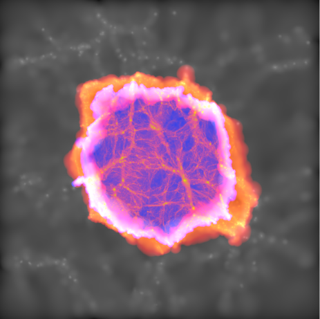
Figure 1: Projected density along the z-axis of a $70.4\times 70.4\times 1.5h^{-1}\,{\rm Mpc}$ slice centred on the middle of the coco simulation at redshift $z=0$. The various colours show the density at different resolution levels: lowest resolution (grey), medium resolution (orange and purple) and high-resolution (blue to yellow). Note the amazing level of the cosmic web details seen inside the high-resolution region.

The coco simulation was designed with the goal of resolving the formation and evolution of MW-size haloes and their subhaloes in a representative cosmological volume. This prompted the use of a zoom-in simulation (Katz & White, 1993; Frenk et al., 1996; Crain et al., 2009; Oñorbe et al., 2014) that captures in very great detail the evolution of a selected region, which in turn is embedded within a larger cosmological volume that is simulated at low-resolution. The role of the latter is to produce the correct large scale modes and tidal fields inside the high-resolution region. Starting from a low-resolution simulation, the high-resolution volume was selected by optimizing the number of Galactic-mass haloes that could be resolved given the available computational resources.

Randomly selecting the high-resolution region can result in it containing one or more rich clusters. Such massive objects would dominate the computational time required for the whole coco simulation, leading to a wastage of resources, since we are primarily interested in MW and lower mass objects. To avoid unnecessary computations, but keeping in mind that we want to simulate a fair-sample of the Universe, possibly close to the observed Local Volume, we have selected a region that satisfies the following criteria:

1. there are no cluster-mass haloes ($M\stackrel{{\scriptstyle>}}{{{}_{\sim}}}5\times 10^{13}h^{-1}{\rm M}_{\odot}$) inside the zoom-in region,

2. there are no massive cluster haloes ($M\stackrel{{\scriptstyle>}}{{{}_{\sim}}}5\times 10^{14}h^{-1}{\rm M}_{\odot}$) within $5h^{-1}\,{\rm Mpc}$ of the zoom-in boundary,

3. the mass function of MW-mass haloes ($M\sim 10^{12}h^{-1}{\rm M}_{\odot}$) is as close as possible to the universal mass function.

2.1 Cosmological and numerical parameters

The coco simulation follows structure formation in a high-resolution region that is approximately a sphere of radius $\sim 17.4h^{-1}\,{\rm Mpc}$ ($2.2\times 10^{4}h^{-3}\,{\rm Mpc}^{3}$ in volume) embedded within a $70.4h^{-1}\,{\rm Mpc}$ low-resolution periodic box, as illustrated in Fig. 1. It uses a Wilkinson Microwave Anisotropy Probe (WMAP) - seventh year result cosmogony (Komatsu et al., 2011) with the following cosmological parameters:

$$\Omega_{m0}=0.272\,,\,\,\Omega_{\Lambda 0}=0.728\,,\,\,\Omega_{b}=0.04455\,,$$

$$\Omega_{k}=0\,,\,\,h=0.704\,,\,\,\sigma_{8}=0.81\,,\,\,n_{s}=0.967\,.$$ (1)

The high resolution region consists of ${\sim}12.9$ billion particles of mass $1.135\times 10^{5}h^{-1}{\rm M}_{\odot}$ and of ${\sim}510$ million medium and low resolution particles that have progressively larger masses. The Plummer equivalent force softening was chosen to increase from a value of $0.23h^{-1}\,{\rm kpc}$ for the high resolution particles to a value of $23h^{-1}\,{\rm kpc}$ for the lowest resolution level.

The high-resolution region was selected from a lower resolution version of the coco simulations that we refer to as COpernicus complexio LOw Resolution (color). The color simulation has the same corresponding initial phases as coco but is set-up with $1620^{3}$ DM particles uniformly distributed throughout the whole $70.4h^{-1}\,{\rm Mpc}$ periodic box. It has a mass and force resolution of $\sim 6.2\times 10^{6}h^{-1}{\rm M}_{\odot}$ and $1h^{-1}\,{\rm kpc}$ respectively, which is exactly the same as in the ms-II. While the color box size is relatively small, the lack of very large-scale modes has little impact on the internal properties of galactic and smaller mass haloes (for more details see Power & Knebe, 2006).

The selection of the coco zoom-in region was performed by generating a large number of randomly placed spheres of radius $17h^{-1}\,{\rm Mpc}$ in the color volume at $z=0$. We discarded any volume not fulfilling criteria (i) and (ii) given in Section 2. From the remaining volumes, we selected the one whose halo mass function in the range, $M\lesssim 10^{12}h^{-1}{\rm M}_{\odot}$, showed the closest match to the universal mass function. Following this, the initial conditions of the zoom-in region were generated using the same method as in the aquarius and the gimic (Crain et al., 2009) projects. The particles from the selected $z=0$ volume were traced back to their Lagrangian positions. The Lagrangian volume was divided in $256^{3}$ regular cells and each cell occupied by one or more of these particles was classified as high resolution. The remaining cells were classified as medium or low resolution cells depending on the distance to the nearest high resolution cell. Each high resolution cell is filled with a periodic glass distribution of $24^{3}$ particles, while the medium to low resolution cells were sampled with progressively fewer particles. Higher frequency power was added to the resulting particles down to the Nyquist frequency while making sure that the lower frequency modes were the same as in the color simulation.

The initial conditions (initial positions and velocities of all particles) for the coco simulation were set at $z=127$ using second order Lagrangian perturbation theory using the method of Jenkins (2010). The initial phases for both the coco and color are taken from the public multi-scale Gaussian white noise field called Panphasia, and are published in Table 6 of Jenkins (2013) under the alternative name of the ‘DOVE’ simulation. The coco initial conditions differ from color by a uniform spatial translation so that the coordinate origin in coco is located at the coordinates $(7,16,44)h^{-1}\,{\rm Mpc}$ within the color simulation. This translation places the high resolution region of coco at the centre of the simulation volume.

Table 1: Details of the simulations used and described in this work along with a list of some other large simulations frequently used in the literature. $V_{\rm box}$ gives the total comoving volume of the simulation, $N_{p}$ is the number of N-body particles, $\varepsilon$ denotes the Plummer-equivalent force softening, expressed in comoving units, $m_{p}$ is the mass resolution.

Name	$V_{\rm box}$ [$h^{-3}\,{\rm Mpc}^{3}$]	$N_{p}$	$\varepsilon$ [$h^{-1}\,{\rm kpc}$]	$m_{p}$ [$h^{-1}{\rm M}_{\odot}$]	cosmology	reference
coco	${\sim}2.2\times 10^{4}$	${\sim}2344^{3}$	0.23	$1.135\times 10^{5}$	WMAP7	this work
color	$3.5\times 10^{5}$	$1620^{3}$	1.0	$6.19\times 10^{6}$	WMAP7	this work
Millennium-II	$1.0\times 10^{6}$	$2160^{3}$	1.0	$6.89\times 10^{6}$	WMAP1	Boylan-Kolchin et al. (2009)
Millennium	$1.3\times 10^{8}$	$2160^{3}$	5.0	$8.61\times 10^{8}$	WMAP1	Springel et al. (2005)
aquarius lvl. 31	${\sim}1.1\times 10^{2}$	${\sim}530^{3}$	$0.12$	${\sim}5\times 10^{4}$	WMAP1	Springel et al. (2008)
Via Lactea (LR)1	${\sim}5.5\times 10^{2}$	${\sim}402^{3}$	0.378	$4.11\times 10^{5}$	WMAP3	Diemand, Kuhlen & Madau (2007)
Horizon-$4\pi$	$8.0\times 10^{9}$	$4096^{3}$	7.6	$7.7\times 10^{9}$	WMAP3	Teyssier et al. (2009)
Bolshoi	$1.6\times 10^{7}$	$2048^{3}$	1.0	$1.35\times 10^{8}$	combination	Klypin, Trujillo-Gomez & Primack (2011)
Horizon Run 3	$1.3\times 10^{12}$	$7210^{3}$	150	$2.44\times 10^{11}$	WMAP5	Kim et al. (2011)
Jubilee	$2.2\times 10^{11}$	$6000^{3}$	no data	$7.49\times 10^{10}$	WMAP5	Watson et al. (2014)
MICE	$2.9\times 10^{10}$	$4096^{3}$	50	$2.93\times 10^{10}$	WMAP5	Fosalba et al. (2015)

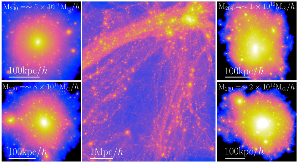
Figure 2: A selection of non-linear structures from the coco simulation. The left- and right-hand panels show the projected DM density for four MW-mass FOF haloes. The central panel gives the projected DM density (in a $1.5h^{-1}\,{\rm Mpc}$ thick slice) in a region that clearly illustrates the rich hierarchy of non-linear structures resolved in coco, from massive haloes (upper-right corner) to cosmic web filaments and voids.

The coco and color simulations were both run with gadget3 Tree-PM N-body code, which is an updated version of the publicly available gadget2 code (Springel, 2005). gadget3 is a hybrid code in which the long-range forces are computed using a particle-mesh method, while short-range forces are obtained by using a hierarchical oct-tree algorithm. This particular heterogeneous architecture allows for a relatively easy follow-up of nested grids placed with increasing accuracy around the high-resolution region. This results in a proper long-range force accuracy throughout the box, while focusing most of the computational effort inside the high-resolution region of interest. For both simulations DM particle positions and velocities were saved in 160 equally spaced in $log(z+1)$ snapshots. Table 1 summarizes some details of the coco and color simulations and compares these with some other widely used cosmological simulations.

2.2 Halo and subhalo finding

We identified DM haloes and subhaloes using the subfind algorithm (Springel et al., 2001). Due to the large number of particles and high clustering level of the coco simulation, the standard version of subfind would have required a vast amount of computer memory and CPU time. To overcome this problem, we have used an updated version of the algorithm that has been especially optimised for parallel computing and big data. While these changes significantly decrease the required computational resources, they do not affect the final output of the method, with the new subfind version producing the same halo and subhalo catalogues as the older version.

subfind starts by identifying DM haloes using the friends-of-friends (FOF) algorithm (Davis et al., 1985), for which we used a linking length $b=0.2$ times the mean inter particle separation. If any resulting FOF group has one or more low resolution particles, we exclude it from further analysis since the internal properties of such objects might have been affected by unrealistic two-body scattering and self gravity. All pristine FOF groups with at least 20 particles were kept for further analysis. At $z=0$ we found more than $1.2\times 10^{7}$ ($5.18\times 10^{6}$) FOF groups in the coco (color) run, with the peak value was found at $z=3$ and consisted of $1.63\times 10^{7}$($6.19\times 10^{6}$) groups. subfind further analyses each FOF group to find gravitationally self-bound DM subhaloes (i.e. substructures within the FOF groups). Subhalo candidates are first identified by looking for overdense regions inside the FOF groups that are further pruned by checking which ones are gravitationally self-bounded objects. This results in a catalogue of self-bounded structures containing at least 20 particles. For each subhalo we also compute and store a number of additional properties. This consists of peak circular velocity, $V_{max}$, and the physical radius, $R_{max}$, at which this peak is attained, half-mass radius, spin (angular momentum), position (corresponding to the minimum of gravitational potential) and bulk velocity of the subhalo.

Each subhalo is characterised by a well defined mass, $M_{sub}$, and radius, $r_{sub}$. The former is given by the mass contained in all the particles that pertain to the subhalo. The latter is approximately the subhalo proper tidal radius (see Figure 15 of Springel et al. (2008)). The FOF groups are characterised in terms of their FOF mass, $M_{FOF}$, as well as of their $M_{200}$ mass. The first, similarly to subhaloes, is given by the mass contained in all the particles associated to a given FOF group. In contrast, $M_{200}$ is the mass contained in a sphere of radius $r_{200}$ centred on the FOF group, such that the average overdensity inside the sphere is $200$ times the critical closure density, $\rho_{c}$. We refer the reader to Sawala et al. (2013) for a comparison of systematic differences between the two as well as other halo mass definitions.

To compute the radial profiles of haloes, we follow a prescription similar to that employed by Power et al. (2003) and Knollmann & Knebe (2009). Namely, we identify the centre of mass of FOF groups using an iterative procedure, by computing the centre of mass inside smaller and smaller spheres, with each such sphere centred on the centre of mass found in the previous iteration step. The centre of each FOF group is used to grow logarithmically spaced spherical shell bins up to $r_{200}$. Figure 2 illustrates the level of detail to which we resolve MW-mass FOF haloes.

2.3 Merger Trees

In CDM cosmologies the first objects to from are DM clumps (haloes) with Jeans mass of the order of Earth mass $\sim 10^{-6}\textrm{M}_{\odot}$ (see e.g. Green, Hofmann & Schwarz, 2004). Due to numerical limitations, such small density perturbations are not resolved in our simulations, hence the first objects to from in coco have masses of $\sim 10^{6}h^{-1}{\rm M}_{\odot}$, some 12 orders of magnitude larger. However, it is well established (e.g. Lacey & Cole, 1993; Kauffmann & White, 1993; Roukema et al., 1997) that in hierarchical cosmologies characterised by a nearly scale-free Harrison-Zeldovitch like (Harrison, 1970; Zeldovich, 1972) initial power spectrum, such as $\Lambda{\rm CDM}$, larger objects forms by consecutive merging of smaller ones. Successive populations of haloes grow from mergers of earlier populations accompanied by accretion of some smooth mass component (see e.g. Wechsler et al., 2002). In order to trace the temporal evolution of haloes we constructed DM haloes merger trees (for more details see Helly et al., 2003). For this, we employed a recently updated algorithm that has been developed for use with the semi-analytic galaxy formation code GALFORM (Cole et al., 2000). The method we used is described in detail in Jiang et al. (2014) and is an upgrade over the earlier version of Merson et al. (2013). The essential part of the algorithm consists of unique linking between subhaloes from two consecutive snapshots. This allows for a construction of very precise merger trees at the subhalo level. We have applied this algorithm to the coco simulation, resulting in approximately $1.312\times 10^{9}$ unique subhaloes contained in the merger trees.

3 Dark Matter haloes

In this section we focus on a few key aspects of DM haloes: their abundance as a function of mass, their internal structure and their formation histories. Understanding the basic properties of DM haloes is a key ingredient of any successful galaxy formation theory, since galaxies are formed and evolve inside their host haloes. Furthermore, understanding the link between the properties of DM haloes and the luminous galaxies that reside within them is crucial for designing and conducting astrophysical tests of the $\Lambda{\rm CDM}$ paradigm.

3.1 Mass function

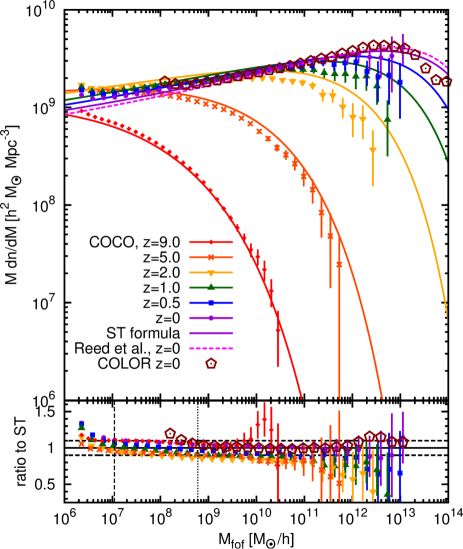
Figure 3: Upper panel: FOF mass functions for the coco and the color simulations, on which we superimpose the Sheth-Tormen prediction (solid lines). The coco results and the ST predictions are plotted for a wide range of redshifts, from $z=9$ (red diamonds) to $z=0$ (purple circles). For comparison we also plot the $z=0$ results from the color run (open hexagons) and the Reed et al. prediction (dashed line). The vertical bars indicate Poisson errors. Bottom panel: The coco and color mass functions normalized by the ST prediction at that redshift. The horizontal dashed lines mark a $10\%$ difference level. The vertical dashed (dotted) line illustrate the coco (color) halo mass resolution limit.

Accurate theoretical predictions for halo mass functions are needed for a number of reasons. For example, they are a primary input for modelling galaxy formation, whether it be physically motivated semi-analytical models (e.g. Cole et al., 1994, 2000) or statistical-based approaches like abundance matching (e.g. Yang, Mo & van den Bosch, 2003; Guo et al., 2010). The abundance of haloes across cosmic epochs was studied since the early work of Press & Schechter (1974), with predictions resulting from the extended excursion set models based on ellipsoidal collapse (Sheth & Tormen, 2002) or motivated by N-body simulations (e.g. Jenkins et al., 2001; Warren et al., 2006; Reed et al., 2007). Such models were thoughtfully tested in computer simulations, but only in a limited mass range $M_{\rm FOF}>\textrm{a few}\times 10^{8}h^{-1}{\rm M}_{\odot}$. Due to our unique coco and color simulations, we are able to investigate the abundance of FOF haloes down to lower masses and over a wide range, spanning 8 decades in halo mass.

In Figure 3 we compare the present day coco and color halo mass function with the Sheth&Tormen (ST) prediction (Sheth & Tormen, 2002) and with the improvement suggested by Reed et al. (2007, hereafter R07), which was tuned using results of N-body simulations. The R07 prediction includes the dependence of the halo mass function on the effective power spectral slope ($n_{eff}$) at the scale of the halo radius. We find good agreement between the present day coco and color mass functions all the way from the resolution limit of the color simulation, $M_{\rm FOF}\sim 6\times 10^{8}h^{-1}{\rm M}_{\odot}$, up to the most massive objects found in the coco volume, $M_{\rm FOF}\sim 10^{13}h^{-1}{\rm M}_{\odot}$. As the resolution limit of FOF haloes we adopt a minimum threshold of 100 particles. Note that this is different from the resolution limit of converged internal (sub)halo properties (e.g. $V_{max}$) that we derive in Appendix A. This assures as that the specific choice of the coco region (see §2) did not introduce any significant halo abundance bias (scarcity or excess) for the range of halo masses that we are interested in. We also see a good agreement with the ST and R07 models at $z=0$, though both coco and color predict slightly more low mass haloes. This discrepancy is rather small, for example at a halo mass of $10^{7}h^{-1}{\rm M}_{\odot}$, where the difference is the largest, ST predicts a $\sim 11\%$ lower halo abundance, while the R07 result is $\sim 18\%$ lower. These differences are unlikely to be caused by numerical effects. First, while it is well known that the FOF algorithm tends to overpredict the abundance of poorly resolved haloes, this effect is significant only for objects with fewer than 100 particles (Warren et al., 2006).

Figure 3 also shows the time evolution of the coco halo mass function from redshift $z=9$ till the present day. The result beautifully reflects the well known hierarchical character of DM halo build-up, with smaller haloes forming first, which in turn merge into bigger and bigger objects. For comparison for each coco redshift data we also plot the ST prediction line. It is clear that the ST prognosis fails to match the coco data for $0.5\leq z\leq 5$ as it significantly overpredicts the abundance of objects. Similar results were also found by Klypin, Trujillo-Gomez & Primack (2011). Interestingly this discrepancy is largest for the intermediate redshifts of $1\stackrel{{\scriptstyle<}}{{{}_{\sim}}}z\stackrel{{\scriptstyle<}}{{{}_{\sim}}}2$, while at $z=9$ the ST forecast is again in a good agreement with our data. The epoch at which we observe the biggest discrepancy between the coco data and the ST predictions also happens to be the epoch at which the halo merger rates are the highest (see e.g. Hopkins et al., 2010), hence the mass function of collapsed objects experience the most dynamical evolution, which in turn is reflected in the failure of the ST forecast.

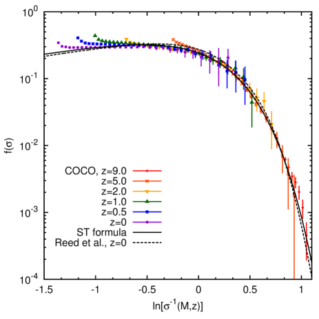
Figure 4: FOF halo multiplicity function, $f(\sigma)$, as a function of peak mass variance, $\sigma(M,z)$, for a range of redshifts. The vertical bars indicate Poisson errors.

To better compare with analytical models for the abundance of haloes, it is more convenient to express the halo mass, $M$, in terms of the variable ${\rm ln}\,[\sigma^{-1}(M,z)]$, where $\sigma(M,z)$ gives the peak mass variance at scale $M$ and redshift $z$. This quantity is defined as

$$\sigma^{2}(M,z)={1\over 2\pi^{2}}\int P(k,z)W^{2}(k,M)k^{2}\textrm{d}k\,,$$ (2)

where $P(k,z)$ is the power spectrum of linear density fluctuations extrapolated to redshift $z$ and $W(k,M)$ is the Fourier transform of the top-hat window corresponding to the radius enclosing mass $M$ at the mean density of the universe. Now, the halo mass function can be written as

$$M{\textrm{d}n(M,z)\over\textrm{d}M}=\overline{\rho}(z){\textrm{d}{\rm ln}\,\sigma^{-1}\over\textrm{d}M}f(\sigma)\,,$$ (3)

where $\overline{\rho}(z)$ is the mean mass density of the universe at redshift $z$ and $f(\sigma)$ denotes the halo multiplicity function. This latter quantity, $f(\sigma)$, takes a universal form that is independent of redshift (for more details, see Jenkins et al., 2001; Reed et al., 2007; Tinker et al., 2008; Angulo et al., 2012). In Figure 4 we plot the multiplicity function of FOF haloes as a function of ${\rm ln}\,[\sigma^{-1}(M,z)]$ at various redshifts. Independent of redshift, the data points follow, to a good approximation, the universal shape as predicted by both ST and Reed et al. formulas.

3.2 Density profiles and the mass-concentration relation

Spherically averaged radial density profiles are one of the simplest yet robust characterisations of the internal structure of DM haloes. It is well established that for hierarchical cosmologies like CDM, the radial density profile of relaxed DM haloes is to a good approximation self-similar and can be mapped by a simple broken power-law formula, the NFW profile (Navarro, Frenk & White, 1996, 1997):

$${\rho(r)\over\rho_{crit}}={\delta_{c}\over(r/r_{s})(1+r/r_{s})^{2}}\,.$$ (4)

It characterises the profile of any halo by two parameters: a scale radius, $r_{s}$, and a characteristic overdensity, $\delta_{c}$. Instead of working with the $r_{s}$ and $\delta_{c}$ parameters, it is customary to define the halo concentration, $c_{200}$, as:

$$c_{200}={r_{200}\over r_{s}}\,,$$ (5)

with $r_{200}$ the virial radius of the halo defined in §2.2. Using this parametrisation, the NFW profile effectively becomes a one parameter fit, since the characteristic overdensity can be expressed as:

$$\delta_{c}={200\over 3}{c_{200}^{3}\over{\rm ln}\,(1+c_{200})-c_{200}/(1+c_{200})}\,.$$ (6)

The density profile of a halo is also probed by the shape of the circular velocity curve, which is:

$$V_{c}(r)=\sqrt{{\textrm{G}M(<r)\over r}}\,,$$ (7)

where $M(<r)$ is the mass contained inside a sphere of radius $r$ centred at the halo centre. For a perfectly spherical halo, the circular velocity, $V_{c}(r)$, is exactly equal to the circular orbital velocity at distance $r$. For well resolved and relaxed haloes, the circular velocity takes only one maximum value, $V_{max}$, that is attained at radial distance, $R_{max}$. Similar to the virial mass, we can define the virial circular velocity $V_{200}=(\textrm{G}M_{200}/r_{200})^{1/2}$. The circular velocity, $V_{c}(r)$, bears effectively the same information as the halo density profile, $\rho(r)$, but is much less prone to noise because of the integral nature of the former.

The NFW scale radius, $r_{s}$, gives the radial position at which the $r^{2}\rho(r)$ curve attains its maximum, which sometimes is also denoted by $r_{-2}\equiv r_{s}$. For the majority of DM haloes, the peak of the $r^{2}\rho(r)$ curve is relatively broad. This means that, for haloes resolved with a relatively small number of particles, the exact location $r_{-2}$ of the peak is uncertain due to the presence of noise. This is reflected in the susceptibility of the NFW fit to the radial range used for fitting the profile of haloes resolved with fewer than a few thousand particles (Navarro et al., 2004; Prada et al., 2006; Gao et al., 2008; Ludlow et al., 2010). This is especially prominent when profiles of many similar mass haloes are stacked to remove halo-to-halo variation due to the presence of substructures. This behaviour indicates that fitting NFW profiles to haloes resolved with a relatively small number of particles is biased and gives rise to an artificial correlation between concentration and halo mass. As a solution, Navarro et al. (2004) proposed the use of a more flexible parametrization, that would account for the differences between NFW and stacked universal halo profiles. The improved three-parameter fitting formula takes a form, in which the logarithmic slope of density assumes a single power law:

$${\textrm{d}\log\rho(r)\over\textrm{d}\log r}=-2\left({r\over r_{-2}}\right)^{\alpha}\,.$$ (8)

This induces radial density profile of the form:

$${\rm ln}\,(\rho(r)/\rho_{-2})=-(2/\alpha)[(r/r_{-2})^{\alpha}-1]\,,$$ (9)

where $\rho_{-2}$ is the density at $r_{-2}$. The additional parameter $\alpha$ is called the shape parameter and, for CDM haloes, it typically takes values in the range $0.1-0.3$. This power-law density profile was first introduced by Einasto (1965) to model the density distribution of the stellar halo of our own Galaxy. To distinguish this density fitting function from the NFW profile we will refer to it as the Einasto profile. The Einasto profile can be characterised in terms of a concentration parameter that is given by eqn. (5) with $r_{s}$ replaced by $r_{-2}$. Both the Einasto $r_{-2}$ parameter as well as the NFW scale radius, $r_{s}$, correspond to the scale at which the logarithmic slope of the density profile attains the ’isothermal’ value of -2. In addition, for $\alpha\simeq 0.2$ the Einasto profile approximates fairly well the NFW profile in the fit range.

In this work we are interested in a statistical description of DM haloes concentrations, with emphasis on the relation between concentration and halo mass, its variance and its redshift evolution. To obtain robust measurements, we fit both the NFW and Einasto profiles to all the haloes with at least $N^{min}_{p}=5000$ particles, which for coco corresponds to a minimum halo mass, $M^{min}_{200}=5.7\times 10^{8}h^{-1}{\rm M}_{\odot}$. We discuss further down why we picked this particular limiting value. The fitting procedure finds the parameter values that minimize the merit function

$$\sigma^{2}(\vec{\Xi})=N_{bins}^{-1}\sum_{i=1}^{N_{bins}}[{\rm ln}\,\rho_{i}-{\rm ln}\,\rho_{fit}(\vec{\Xi})]^{2}\,,$$ (10)

where the vector of fit parameters $\vec{\Xi}=(r_{s},\delta_{c})$ and $(r_{-2},\rho_{-2},\alpha)$ for the NFW and Einasto fits, respectively. The number of radial bins, $N_{bins}$, is equally spaced in $\log(r)$ and is selected adaptively depending on the number of particles, $N_{p}$, contained in the halo as:

$$N_{bins}=2\textrm{ceiling}(6.2\log{N_{p}}-3.5)\,.$$ (11)

This gives $N_{bins}=92$ for our most massive halo and $N_{bins}=40$ bins for a halo with 5000 particles. Since the bins are equally spaced in $log(r)$, the inner bins contain significantly fewer particles than the mid-range and outer bins. Hence, as we move towards the halo centre, the radial bins become more affected by sampling noise and two body scattering effects. This has been studied by Power et al. (2003), who found that there is a minimum radius below which one cannot trust the radial density profile of haloes extracted from N-body simulations. This convergence radius is given by the inner most bin that fulfils the Power et al. (2003) criterion (see eqn. (20) in their paper). We exclude from the fitting all radial bins that are below the convergence radius for a given halo. After applying this convergence criterion, a halo resolved with $N^{min}_{p}=5000$ particles is left on average with 20 radial bins. Thus, the minimum halo mass for which we perform a fit is given by the mass for which more than a half of the radial bins pass the convergence test.

The individual density profile of haloes resolved with fewer than $N^{min}_{p}=5000$ particles is very sensitive to the intrinsic numerical noise. However, there is still plentiful of information that can be extracted from haloes with fewer than $N^{min}_{p}$ particles. By stacking many such haloes, the noise of the density profile is significantly reduced. Finding the position of the maximum of the $r^{2}\rho(r)$ curve for a such stacked profile gives the $r_{s}$ and $r_{-2}$ parameters for the NFW and Einasto profiles, respectively. We apply this method to get median concentration of stack profiles for haloes with $800\leq N_{p}\leq 5000$. Using this approach, we estimate halo concentrations in coco down to a halo mass of $M_{200}=9\times 10^{7}h^{-1}{\rm M}_{\odot}$.

The NFW and Einasto profiles represent a good description of the radial density profiles for virialised DM haloes, which are in equilibrium. Haloes that experienced recent mergers or close encounters can be far away from the state of equilibrium and, thus, their density profiles are usually not very well described by neither NFW nor Einasto profiles. As a consequence, the concentration parameter derived from fitting unrelaxed haloes is ill defined and at best biased low (see e.g. Neto et al., 2007; Gao et al., 2008; Ludlow et al., 2010). To overcome this problem, we remove non-virialised haloes, i.e. objects that do not satisfy the following three criteria (Neto et al., 2007): (i) the fraction of halo mass contained in its resolved substructure is $f_{sub}<0.1$, (ii) the displacement between the centre of mass and the minimum of the gravitational potential cannot exceed $7\%$ of halo’s virial radius, $r_{200}$, and (iii) we require that the adjusted virial ratio, $\nu\equiv(2T-E_{s})/|U|$, is $\nu<1.35$. Here $T$ and $U$ are the halo’s total kinetic and potential energy, respectively. To account for the fact that real haloes are not isolated objects, we include the Chandrasekhar pressure term, $E_{s}$, which quantifies the degree to which a given halo interacts with its surroundings. See Shaw et al. (2006) and their eqn. (6) for the definition and method used to estimate the pressure term, and also see Power, Knebe & Knollmann (2012) for a more detailed discussion about the virial ratio of haloes.

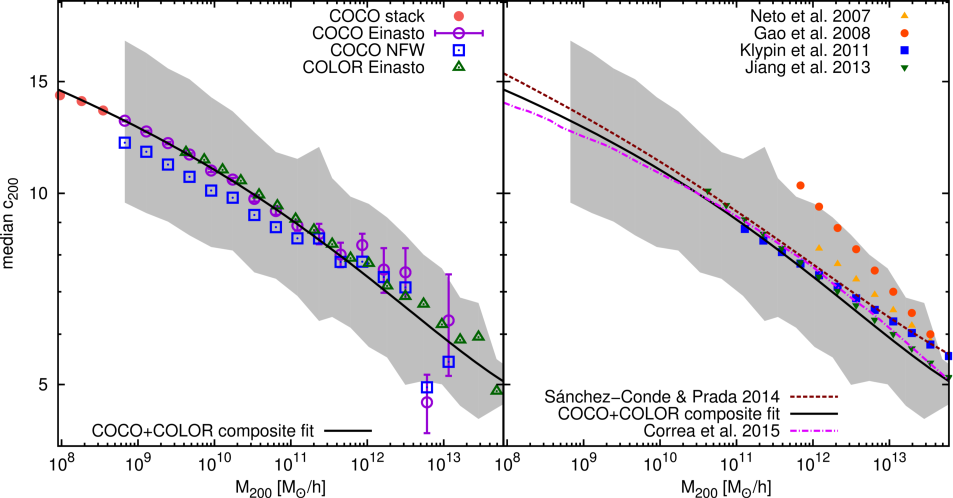
Figure 5: Left-hand panel: Concentration-mass relation for relaxed haloes. The open symbols give the median concentration obtained from fitting NFW and Einasto profiles. The best-fitting line was obtained from the combined Einasto coco+color data, with the coco concentrations (circles) extended by the color results (triangles) for halo masses $M_{200}>5\times 10^{11}h^{-1}{\rm M}_{\odot}$. The filled circles show the average concentrations obtained from stacking profiles for the three lowest mass bins. For comparison we also show the data obtain by fitting the NFW profile (open boxes). Right-hand panel: Comparison of various $c_{200}-M_{200}$ fits from the literature (lines with symbols and the dashed line) with our best-fitting line (solid line). In both panels, the shaded region shows the 16th to 84th percentile scatter of the coco+color data.

The left-hand panel of Figure 5 shows the median halo concentration as a function of halo mass for our two simulations, coco and color. We find a very good agreement between coco and color results for all halo masses up to $M_{200}\sim 3.5\times 10^{12}h^{-1}{\rm M}_{\odot}$. Above this mass, due to scarcity of the massive haloes, the coco results are dominated by halo-to-halo scattering. This is clearly seen from the increasing size of the error bars that show the bootstrap errors of the median. The good agreement between the two simulations suggests that we can supplement the coco data at the high-mass end by adding the objects from the color simulation. We construct such a joint sample and use it for obtaining our best-fit for the median $c_{200}-M_{200}$ relation as discussed later. Comparing the results for the NFW and Einasto fits, we find clear differences between the two. Below a halo mass of $M_{200}\lesssim 10^{11}h^{-1}{\rm M}_{\odot}$, the difference takes the form of a systematic shift, with the slope of the $c_{200}-M_{200}$ relation being similar for both profile fits.

In the right-hand panel of Figure 5 we also show various fits to the $c_{200}(M_{200})$ relation with the goal of comparing the accuracy of these literature fits with the results of N-body simulations. From the set of single power-law fits, the one that best matches the data is the fit proposed by Jiang et al. (2014). This is in very good agreement (better than $4\%$) with both coco and color data down to a halo mass of $\sim 2\times 10^{10}h^{-1}{\rm M}_{\odot}$. It seems that below that mass our data indicate slight flattening of this relation, hence change of the slope. Also the fit of Klypin, Trujillo-Gomez & Primack (2011) is in a reasonably good agreement with our data, except for the most massive objects ($\sim 5\times 10^{13}h^{-1}{\rm M}_{\odot}$) where it predicts a median concentration that is higher from the value of $84\%$ of our haloes at that mass. The Klypin et al. results were found for halo masses and boundaries defined by a spherically averaged overdensity $\Delta_{vir}=360\times\Omega_{m,0}\times\rho_{c}$. This definition roughly corresponds to $\Delta_{100}$ in our nomenclature, hence, to allow for a comparison of their fit with our data, we have rescaled their $c_{vir}-M_{vir}$ relation to appropriate equivalent of $c_{200}-M_{200}$. However, this procedure ideally should be performed for each halo separately at the particle level, so our rescaling here can only be treated as an approximation. The performance of the Neto et al. (2007) fit is also reasonably good down to $M_{200}\sim 10^{12}h^{-1}{\rm M}_{\odot}$. The fit of Gao et al. (2008) agrees with our data only for the most massive bins and it clearly predicts a different slope of the concentration-mass relation. This unavoidably leads to a significant overestimation of the median halo concentration by their fit for haloes below a mass of $\sim 2\times 10^{12}h^{-1}{\rm M}_{\odot}$. There are two possible sources driving this discrepancy. First, the Gao et al. fit is based on the ms which uses significantly different values of the cosmological parameters. This difference is most notable for the $\sigma_{8}$ parameter that is $10\%$ higher in the ms than in our simulations. The different cosmology is probably the main reason for the observed differences since variations in both $\Omega_{m}$ and $\sigma_{8}$ have a large impact on halo concentrations (Ludlow et al., 2013; Dutton & Macciò, 2014; Diemer & Kravtsov, 2015). Secondly, the Gao et al. relation is obtained by fitting a relatively limited halo mass range given by $5\times 10^{12}\leq M_{200}/(h^{-1}{\rm M}_{\odot})\leq 10^{15}$. Since the concentration-mass relation is not a simple power law, fitting a single power law provides a relation that holds only for that mass range (Ludlow et al., 2014; Sánchez-Conde & Prada, 2014; Prada et al., 2012).

Table 2: Our best-fitting parameters for the $c_{200}-M_{200}$ relation for the functional from of the Eqn.(12).

$c_{0}$	$c_{1}$	$c_{2}$	$c_{3}$	$c_{4}$	$c_{5}$
34.988	-1.9841	$8.039\times 10^{-2}$	$-1.777\times 10^{-3}$	$-1.4557\times 10^{-5}$	$7.34152\times 10^{-7}$

To emphasise this last point, we also checked the performance of the multi power-law median $c_{200}(M_{200})$ model of Sánchez-Conde & Prada (2014, hereafter SC14), based on a functional form proposed by Lavalle et al. (2008):

$$\langle c_{200}(M_{200},z=0)\rangle_{med}=\sum_{i=0}^{5}c_{i}\times[{\rm ln}\,(M_{200}/h^{-1}{\rm M}_{\odot})]^{i}\,.$$ (12)

This multi-component fit is claimed to be a much better match for the median halo concentration-mass relation due to flattening of this relation at small halo masses. Not surprisingly, the SC14 fit shows a very good agreement with the N-body results to an accuracy better than $10\%$. However, the SC14 fit systematically overpredicts the median concentration for our haloes with $M_{200}<10^{11}h^{-1}{\rm M}_{\odot}$. Especially for the first four to five least massive bins, we can notice the difference of varying slope of the concentration-mass relation between the SC14 fit and our coco+color sample. To better quantify this discrepancy, we have fitted eqn. (12) to a combination of coco+color data. This ’coco+color composite’ set was obtained by augmenting the coco data for halo masses above $5\times 10^{11}h^{-1}{\rm M}_{\odot}$ with the color data and further supplementing it at the low-mass end with the data obtained from the profile stacking. Our best fitting parameters are presented in the Table 2 and the corresponding fit is marked as a solid black line in Fig. 5. To fix the asymptotic freedom of the fit at the low-mass tail, we have used the data points from Diemand, Moore & Stadel (2005); Ishiyama et al. (2013) and Anderhalden & Diemand (2013). For haloes with $1\lesssim M_{200}/(h^{-1}{\rm M}_{\odot})\lesssim 10^{6}$ our fitted relation predicts concentrations that are $\sim 10\%$ lower than the SC14 fit, while for even smaller haloes this tendency flips and our fit predicts concentrations that are systematically higher. However, such a difference has only small effects on the predicted boost factors for the radiation flux of DM annihilation. For completeness, we also compare the median coco $c(M_{200})$ relation with the model of Correa et al. (2015c) (hereafter C15) which is based on the mass accretion history of haloes (see also Correa et al., 2015a, b; Ludlow et al., 2014). The prediction of the C15 model for a WMAP7 cosmology is shown in the right-hand panel of Fig. 5 as the dashed-dotted line. This model agrees to better than $5\%$ with our data for haloes more massive than $\sim 10^{9}h^{-1}{\rm M}_{\odot}$. At lower masses, the model underpredicts the concentration, which most likely reflects the fact that the C15 model was built for NFW profiles rather than for Einastio profiles.

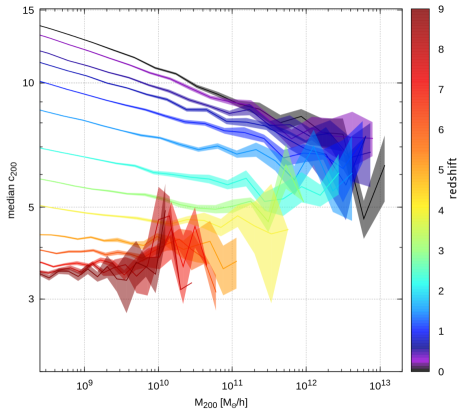
Figure 6: The redshift evolution of the concentration-mass relation for relaxed haloes in the coco volume. We plot the data from $z=9$ (red colour) down to $z=0$ (black). Solid lines mark the median Einasto concentration, while the filled regions show the $1\sigma$ uncertainty in the relation.

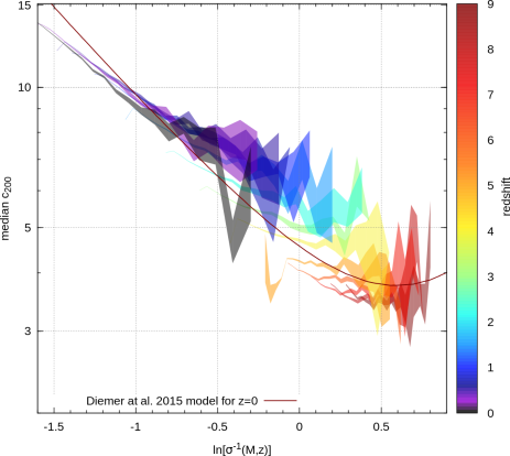
Figure 7: The halo concentration, $c_{200}$, as a function of peak mass variance, $\sigma(M,z)$, for relaxed coco haloes. We show the relation at various redshifts, from $z=9$ (red) down to $z=0$ (black). The black solid line gives the prediction of the Diemer & Kravtsov (2015) model at $z=0$.

In Figure 6 we depict the time evolution of the concentration-mass relation. For $z\gtrsim 2$, we find a flattening of the relation at the high mass end, with the flattening moving towards lower masses for higher redshifts. The same flattening is present also at $z\simeq 0$, but we do not see it in the coco data since the simulation does not resolve very high mass haloes. The concentration is related to the characteristic density of a halo, which in turn reflects the mean density of the universe at the time when the central part of the halo has collapsed (e.g. Gao et al., 2008; Ludlow et al., 2014). This naturally leads to the observed flattening of the $c(M,z)$ relation for very rare and massive objects, since these have assembled only recently and therefore share the same collapse time. We also find an evolution in the slope of the relation for lower mass haloes. This is in agreement with the well established picture according to which haloes are build-up hierarchically. Haloes continuously increase their mass with time, so the concentration at fixed halo mass is determined by different objects for each redshift bin. To better understand the time variation of the halo mass-concentration relation, we express the halo mass in terms of the mass variance, $\sigma(M,z)$ (see Eqn. (2)). The corresponding median $c[\sigma^{-1}(M,z)]$ relation is given in Figure 7 and shows that at fixed $\sigma(M)$ values the concentration varies only slowly with time. For comparison, we also give the prediction of the Diemer & Kravtsov (2015) model to find that in the ‘big-peak’ regime (haloes corresponding to rare peaks at a given epoch) our results are in reasonable agreement with their prediction. At small $\sigma^{-1}(M,z)$ values our data suggest a less steeper slope. The difference can be accounted for by noting that Diemer & Kravtsov (2015) have used a different halo finder and that their simulations had much lower mass resolution, hence they could not probe the ’very small halo’ regime, which our simulation resolves.

3.3 Formation times

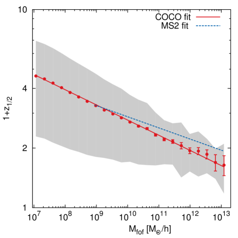
Figure 8: The mean half-mass formation time, $z_{1/2}$, as a function of present day halo mass,$M_{FOF}$. The red points are the simulation data with error bars reflecting the bootstrap error on the mean. The shaded grey region marks the $1\sigma$ scatter around the mean. The solid lines illustrate the fit to the coco (red line) and to the ms-II (blue line) data.

The highly hierarchical character of structure formation is especially strongly imprinted in the build-up and mass accretion histories of dark haloes. A significant fraction of a halo’s mass is assembled via the accretion of other haloes so it is natural to expect that more massive objects form later than the low mass ones, as confirmed by many N-body simulations of the CDM model. However, the precise form of the halo mass-formation time relation and its intrinsic scatter is still a subject of discussion(Lacey & Cole, 1993; Wechsler et al., 2002). Determining this relation is relevant for a number of reasons. Among which, most importantly, is understanding how well this relation is correlated with the properties of the galaxies and the haloes they reside within, which is crucial for all models of galaxy formation (e.g. Cole et al., 2000; Benson et al., 2003; Bower et al., 2006; De Lucia & Blaizot, 2007; Guo et al., 2013).

The simplest and most used definition of the halo formation time, $z_{f}$, is given as the epoch at which a halo’s main progenitor assembles a fixed fraction of the present day halo mass. To compute this, we follow the main progenitor branch of each halo merger tree (see §2.3 for details on the merger trees) until the main progenitor reaches half of the halo’s final mass. Thus, our halo formation time is the redshift of half-mass assembly, $z_{1/2}$. This half-mass formation time is one of the most commonly used formation time definition found in the literature (however see Li, Mo & Gao, 2008, for other possible definitions). Figure 8 shows the formation time as a function of halo mass for our N-body simulations. For comparison, we also show the fit to the relation obtained by Boylan-Kolchin et al. (2009) for ms-II haloes (rescaled from their $M_{vir}$ to our mass definition $M_{FOF}$) and a fit to our own data. For the latter we use the same linear fit in $\log(1+z_{1/2})$ as Boylan-Kolchin et al. (2009), which takes the form:

$$1+z_{1/2}=A_{0}\left({M_{FOF}\over 10^{10}h^{-1}{\rm M}_{\odot}}\right)^{\beta}\,.$$ (13)

The best fit to our data was obtained for $A_{0}=2.77$ and $\beta=-0.0765$ and, as can be seen from the figure, it provides a very good description of the data over the entire mass range.

Compared to the ms-II result we find that our haloes formed at similar epochs, however our formation time-mass relation is steeper. The difference can be presumably accounted for by the different cosmology and due to different mass definitions. Most likely, the higher value of the $\sigma_{8}$ used in the ms-II is a major driver of the discrepancy, as it is well established that this parameters is strongly correlated with the abundance of very massive haloes and hence also with the rate of their mass assembly.

Figure 8 illustrates another important point. The halo-to-halo variation in formation times depends on halo mass, being the largest for low mass haloes and decreasing with increasing halo mass. This trend in halo-to-halo scatter can be understood in light of halo assembly bias, which was first pointed out by Gao & White (2007). The halo assembly bias (see also Croton, Gao & White, 2007; Li, Mo & Gao, 2008) states that the halo formation time, $z_{f}$, is negatively correlated with the local amplitude of the density clustering. It indicates that haloes form earlier in higher-density locations, which naturally have higher clustering amplitudes. Spatial regions characterised by a higher local amplitude of the density field lead to a faster DM halo formation for a number of reasons: (i) because of the excess matter clustering haloes can accrete more mass in the same unit of time, when compared to field haloes; (ii) higher clustering amplitudes imply also higher halo merger rates; (iii) the increased local density (compared to the universal background value) allows some density peaks to reach more rapidly the critical density threshold, $\delta_{c}$, required for collapse. This reasoning can be inverted, when applied to regions with lower clustering amplitude than the mean, where exactly the opposite processes will induce later halo formation times. Another crucial ingredient is that DM haloes are biased tracers of the underlying DM density field (e.g. Frenk et al., 1985; Davis et al., 1985; Frenk et al., 1988; Cole & Kaiser, 1989), with high-mass haloes having a large positive bias, while low mass haloes are slightly anti-biased (prefer to reside in lower-density environments). Thus, massive haloes can only be found in regions characterised by a significant clustering excess. These regions are the nodes and the filaments of the cosmic web (see e.g. Bond, Kofman & Pogosyan, 1996; Sheth & van de Weygaert, 2004; Springel, Frenk & White, 2006; Aragón-Calvo, van de Weygaert & Jones, 2010), which is the most salient observational characteristic of the anisotropic nature of gravitational collapse. In contrast, the lower mass haloes pervade the whole range of large-scale environments, from voids to cosmic nodes, spanning many orders of magnitude in characteristic density (for the most recent results see e.g. Cautun et al., 2014c; Metuki et al., 2015; Falck et al., 2014; Nuza et al., 2014). A detailed investigation of the origin and properties of the halo assembly/cosmic web bias down to the smallest accessible halo mass is needed, in order to obtain a better physical understanding of this mechanism and its implication for halo properties and galaxy formation. In principle the coco simulation set, owing to its resolution and volume, is very-well suited for such studies. However, this venture is beyond the scope of this paper and we leave it for future work.

4 Dark Matter subhaloes

In hierarchical CDM cosmologies, a significant fraction of halo mass growth takes place via the accretion of lower mass haloes, which results in a rich substructure of orbiting smaller DM clumps called subhaloes. The spatial distribution and abundance, kinematic and internal properties, and orbit parameters of these subhaloes are subject of intensive study in modern cosmology. Rendering a firm insight into the various physical properties of subhaloes plays a pivotal role in linking the observed properties of Galactic satellites and dwarf galaxy population of the Local Group to the physical nature of dark matter. In this section we study the properties of the DM as a function of the mass of their host halo.

4.1 Mass and velocity functions

It is well known that due to discreteness of N-body simulations, effects like over-merging, two-body scattering, phase-space graining and force softening will affect the internal properties of haloes and subhaloes that are close to the resolution limit of the simulation (see e.g. Shandarin & Zeldovich, 1989; Klypin et al., 1999a; Power et al., 2003; Springel et al., 2008; Abel, Hahn & Kaehler, 2012; Hahn, Abel & Kaehler, 2013). Among others, these effects lower the maximum velocity, $V_{max}$, of small mass objects whose $R_{max}$ is comparable to the gravitational force softening of the simulation. We apply the correction formula proposed by Springel et al. (2008, Eqn. (10) therein), which, to a good approximation, under assumed perfect circular orbits, accounts for this effect. While we have done so for all our haloes and subhaloes, we found that, due to our very high spatial resolution, the correction has negligible effects for the vast majority of objects with $V_{max}\geq 10\rm{kms}^{-1}$ . The subhaloes below this $V_{max}$ limit are strongly affected by numerical effects, as we discuss in detail in Appendix A, and are not considered in our analysis.

Figure 9: Top panel: The mean cumulative number of subhaloes as a function of $\mu\equiv M_{sub}/M_{200}$ binned for different host masses. The coloured solid lines represent hosts from a halo mass of $\langle M_{200}\rangle=10^{13}h^{-1}{\rm M}_{\odot}$ (green) down $\langle M_{200}\rangle=10^{9}h^{-1}{\rm M}_{\odot}$ (brown). The black solid line shows the best-fitting power law function, $N(>\mu)\sim\mu^{-s}$, with $s=0.95\pm 0.01$, found for the most massive host mass bin. The purple dashed line illustrates the scale-free mass function with $s=1$. Bottom panel: The relative ratio of the data in each host mass bin to the coco best-fitting power law model with $s=0.95$.

Table 3: The best-fitting values for the power-law index, $s$ (see Eqn.(14)), describing the subhalo mass function for hosts of different masses.

$\langle M_{200}\rangle$ in $h^{-1}{\rm M}_{\odot}$	$10^{10}$	$10^{11}$	$10^{12}$	$10^{12}$	$10^{13}$	$10^{14}$
$s$	$0.92\pm 0.02$	$0.93\pm 0.01$	$0.94\pm 0.01$	$0.94\pm 0.02$	$0.95\pm 0.01$	$0.97\pm 0.02$

Fig. 9 shows the mean cumulative number of subhaloes as a function of $\mu\equiv M_{sub}/M_{200}$, namely the gravitationally bound subhalo mass in the units of its parent host halo mass. The resolution of our coco run allows us to reliably identify substructure of various size in hosts down to a halo mass of $\sim 10^{9}h^{-1}{\rm M}_{\odot}$. To take full advantage of this, we bin host haloes according to their mass, $M_{200}$, grouping them in five samples: $1-10\times 10^{9}$, $1-10\times 10^{10}$, $1-10\times 10^{11}$, $1-10\times 10^{12}$ and $1-1.5\times 10^{13}h^{-1}{\rm M}_{\odot}$.

To keep consistency with previous works and in order to make fair comparisons, our analysis includes all subhaloes within a radius, $r_{50}$, from the host centre, as adopted in the analysis of the aquarius suite (Springel et al., 2008). The radius, $r_{50}$, is defined as the boundary at which the spherically averaged density reaches a value of $50$ times the critical density for closure. On average, for galactic mass haloes, $r_{50}\simeq 1.66\times r_{200}$, thus, one will find more subhaloes within $r_{50}$ than within $r_{200}$.

The aquarius and Phoenix (Gao et al., 2012) simulations have indicated that the substructure fractional mass function is well fitted over five orders of magnitude by a single power-law:

$$\overline{N}(>\mu)\propto\mu^{-s}\;.$$ (14)

The best-fitting power-law suggests that $s=0.97\pm 0.02$ for the Phoenix haloes and $s=0.94\pm 0.02$ for the aquarius suite. Both simulations have similar resolutions (for their highest level), but simulate host halo samples of different masses. The aquarius hosts have an average mass of ${\sim}10^{12}h^{-1}{\rm M}_{\odot}$, while the Phoenix ones corresponds to a halo mass, $M_{200}\sim$, a few$\times 10^{14}h^{-1}{\rm M}_{\odot}$.

We fitted the same power-law to the substructure fractional mass function for the coco hosts, to obtain the best-fitting $s$ parameter as a function of host mass. The best fitting values and their standard error are given in Table 3 and were obtained by counting subhaloes with more than $100$ particles. The best-fitting power-law function, for our best resolved hosts, which have a median mass, $\langle M_{200}\rangle=10^{13}h^{-1}{\rm M}_{\odot}$, is shown as a solid line in Fig.9. Interestingly, this best-fitting value is found to be exactly in between the aquarius and Phoenix results, with $s=0.95\pm 0.01$, but consistent with those within the fit errors. Table 3 suggests that the power-law exponent, $s$, may increase very weakly with halo mass, but, given the error associated with $s$, this trend is not statistically significant and a much larger study is needed to confirm or disprove such a trend. For a closer examination, we show in the lower panel of Fig. 9 the fractional difference with respect to the coco best-fitting value of $s=0.95$. The panel illustrates that for all mass-binned samples there is a range in $\mu$ for which the fractional difference exhibits an approximately flat region. At low $\mu$, the deviations from a flat shape are driven by numerical resolution effects, while the behaviour observed at $\mu\stackrel{{\scriptstyle>}}{{{}_{\sim}}}3\times 10^{-2}$ reflects the well known exponential cut-off in the mass function of the most massive substructures.

The best-fitting power law exponents, $s$, that we found are close to the case of a scale-free subhalo mass function with the critical value of $s=1$. For $s=1$, each logarithmic bin in $\mu$ has an equal contribution to the total mass in subhaloes, which is logarithmically divergent as $\mu\rightarrow 0$. If the real substructure mass function is described by $s=1$, than a significant fraction of the host mass is contained in subhaloes beyond the resolution limit of our simulation. For our best resolved sample with $\langle M_{200}\rangle=10^{13}h^{-1}{\rm M}_{\odot}$, an average of $7.7\%$ of the host halo mass is contained in resolved substructure. Extrapolating this down to an Earth mass, corresponding to $\mu=10^{-19}$, yields a fraction of $34\%$ mass locked in substructure. This prediction can be used further to yield DM annihilation gamma-ray flux (see e.g. Bergström, Ullio & Buckley, 1998; Gondolo & Silk, 1999). Detailed investigation of this situation is however beyond the scope of this paper and we leave it for the future work.

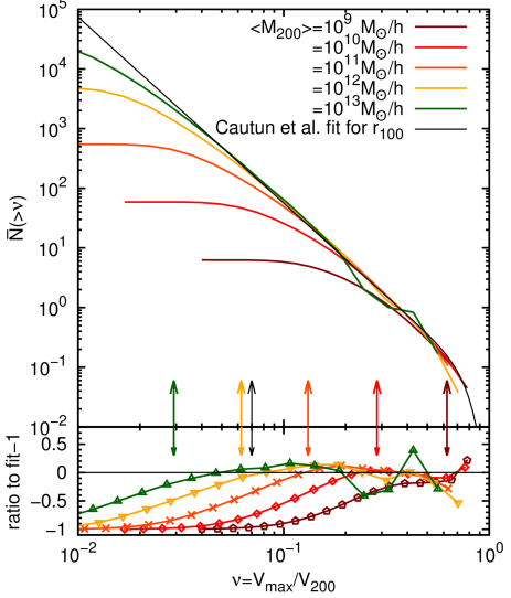
Figure 10: Upper panel: The scaled subhalo maximum circular velocity abundance as functions of the ratio $\nu=V_{max}/V_{200}$ for hosts of different masses. The vertical arrows mark the $\nu$ value corresponding to $V_{max}=10$ kms^-1, which is our resolution limit. The black thin line shows the best-fitting function of Cautun et al. (2014b) for subhaloes within a radius, $r_{100}$, from the host. Lower panel: Ratios between the mean subhalo count at various host masses and the Cautun et al. result.

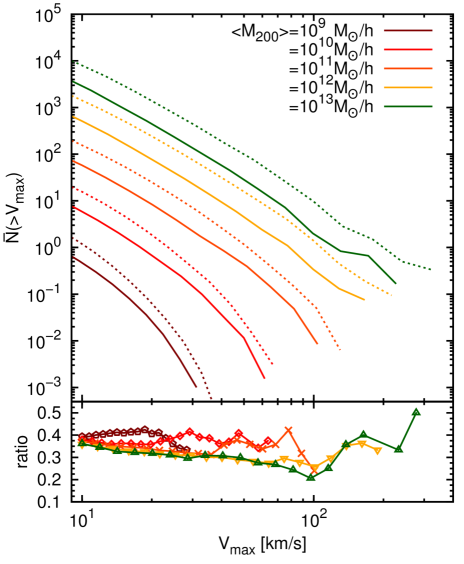
Figure 11: Upper panel: The subhalo count as a function of maximum circular velocity for host haloes of different masses. The solid lines show the subhalo count using the present ($z=0$) $V_{max}$ values. The dotted lines depict the subhalo count using the $V_{max}$ value at the subhalo’s infall time. Lower panel: The ratio between the subhalo count using present time $V_{max}$ and the subhalo count using the $V_{max}$ at infall time.

It has been long postulated that the scaled subhalo velocity function is independent of host halo mass, when expressed as a function of $\nu=V_{max}/V_{200}$, which is the ratio between the subhalo maximum circular velocity and the host virial velocity (e.g. Moore et al., 1999; Kravtsov et al., 2004). Recently, this has been thoroughly confirmed using a large number of host haloes (Wang et al., 2012; Cautun et al., 2014b). Given both the very high resolution and the large number of haloes in the coco simulation, we can investigate the postulated invariance of the scaled subhalo velocity function over a wider dynamical range in subhalo $V_{max}$ and down to lower host halo masses. This is shown in Fig. 10, where we plot the mean cumulative satellite count, $\overline{N}(>\nu)$, as a function of $\nu$ for hosts binned according to their halo mass. To better highlight the invariance with host halo mass, the lower panel of Fig. 10 shows the ratio between $\overline{N}(>\nu)$ measured in coco and the best fit of Cautun et al. (2014b) for the mean subhalo count around galactic mass haloes. Since Cautun et al. (2014b) does not compute the subhalo count within $r_{50}$, we take their result for subhaloes found within a distance of $r_{100}$ from the centre of the host halo. This leads to us counting more subhaloes than Cautun et al. (2014b), which explains why the coco results are systematically above the zero level in the bottom panel of the figure.

We find that the mean subhalo count, $\overline{N}(>\nu)$, exhibits at most a very weak dependence on host mass. This should be compared to the satellite abundances of Fig. 9, which show a strong dependence on host mass, $M_{200}$. Any systematic deviations from a flat line for the results shown in the bottom panel of Fig. 10 appear only below the resolution limit of the simulation, which is show by a vertical arrow for each halo mass bin. The deviations seen at high $\nu$ values for the most massive bin, $M_{200}=10^{13}h^{-1}{\rm M}_{\odot}$, are due to the small number of host haloes present in that sample and hence are not significant. Thus, our results confirm the postulated invariance of $\overline{N}(>\nu)$ over four orders of magnitude in host mass, showing that this assumption holds for the majority of DM haloes that can host galaxies ($10^{10}\stackrel{{\scriptstyle<}}{{{}_{\sim}}}M_{200}h/M_{\odot}\stackrel{{\scriptstyle<}}{{{}_{\sim}}}10^{13}$). This invariance was exploited by Wang et al. (2012) and Cautun et al. (2014a) to derive new theoretical constrains on the mass of the Milky Way halo.

In Fig. 11 we show the mean subhalo count, $\overline{N}(>V_{max})$, as a function of subhalo maximum velocity, $V_{max}$. Describing subhaloes in terms of the maximum circular velocity is more closely related to observations, since $V_{max}$ is more easily measured in observations. The figure compares the subhalo abundance using the present day $V_{max}$ as well as the subhalo count as a function of the maximum circular velocity at subhalo’s infall time, $V_{max}^{inf}$. The $V_{max}^{inf}$ values are obtained by tracing the merger tree of each subhalo and taking the peak value of $V_{max}$ throughout the history of the subhalo. For most practical applications, $V_{max}^{inf}$ is well approximated by the peak value of $V_{max}$, since, once a halo falls into a more massive object, it becomes the subject of intensive tidal stripping and so its $V_{max}$ value is very likely to decrease rather than increase. Fig. 11 shows that at fixed subhalo size, i.e. fixed $V_{max}$ values, the abundance of objects roughly increase by an order of magnitude for each order of magnitude in host mass. This scaling is most pronounced for sufficiently small objects. This scaling breaks down for the most massive subhaloes, since the subhalo abundance changes its shape from a power-law to an exponential decline (see Fig. 9 and  10). Interestingly, a similar scaling is found also for the subhalo abundance as a function of $V_{max}^{inf}$. This can readily be seen from the bottom panel Fig. 11 that shows the ratio $\mathcal{R}=\overline{N}(>V_{max})/\overline{N}(>V_{max}^{inf})$. Both these functions are calculated using the same objects, found at $z=0$ inside a distance, $r_{50}$, from their host, so their values are not influenced by the destruction or accretion of new subhaloes. In other words, we expect that the ratio $\mathcal{R}$ and its departure from unity are a good proxy for the efficiency of subhalo tidal striping at fixed subhalo circular velocity. For small subhaloes with $V_{max}\stackrel{{\scriptstyle<}}{{{}_{\sim}}}20$kms^-1, we find that the ratio approaches $\mathcal{R}\approx 0.35$ for all host masses except for the lowest mass bin. For this lowest mass sample, $\langle M_{200}\rangle=10^{9}h^{-1}{\rm M}_{\odot}$, coco has enough resolution to identify only the most massive subhaloes and it does not capture the power-law like regime of the subhalo abundance function. The convergence of the $\mathcal{R}$ ratios towards a single values indicates that the efficiency of subhalo tidal stripping is comparable in hosts that differ by four orders of magnitude in mass, provided that the considered subhaloes are sufficiently small in comparison to their host.

4.2 The radial distribution

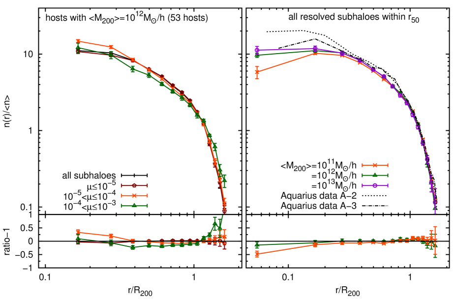
Figure 12: Radial number density profiles of subhaloes. Left panel: The radial distribution of subhaloes in galactic mass hosts, i.e $\langle M_{200}\rangle=10^{12}h^{-1}{\rm M}_{\odot}$. The lines with symbols corresponds to subhaloes of various masses, as expressed in terms $\mu=M_{sub}/M_{200}$, while the black solid line with crosses shows the results for all subhaloes. The bottom panel give the ratio of the various subhalo mass bins with respect to the distribution of all subhaloes. Right panel: The radial distribution of subhaloes for different host masses. The lines with symbols show the results of coco. The dotted line (dashed-dotted) show the equivalent substructure profile from the aquarius A-2 (A-3) run. The bottom panel shows the ratio of each data set to the reference case, which we take as $\langle M_{200}\rangle=10^{13}h^{-1}{\rm M}_{\odot}$.

The radial distributions of subhaloes is also a subject of intensive study (e.g. Gao et al., 2004; Diemand, Moore & Stadel, 2004; De Lucia et al., 2004; Nagai & Kravtsov, 2005; Wang, Frenk & Cooper, 2013), since understanding how DM substructures are distributed inside their host haloes is important for several reasons. Among others, the radial distribution of subhaloes is instrumental in connecting the observations of satellite galaxies with the properties of the background cosmology; it serves as input for many semi-analytical galaxy formation models; and it is important for strong lensing studies (e.g. Mao & Schneider, 1998; Metcalf & Madau, 2001; Metcalf & Zhao, 2002; Kochanek & Dalal, 2004; Xu et al., 2015).

Springel et al. (2008) have found that the radial distribution of subhaloes is independent of subhalo mass for at least five decades in mass (see Fig. 11 therein). We further investigate this finding, since the large number of host haloes of the coco run allow for much better statistics. In addition, we further extended the analysis of Springel et al. by studying how the radial distribution of subhaloes varies with host mass.

The left-hand panel of Fig. 12 shows the dependence of the subhalo radial distribution on subhalo mass. The subhalo population is split according to their rescaled mass, $\mu=M_{sub}/M_{200}$, following which, we stack the radial profiles of 53 host haloes whose median mass is $\langle M_{200}\rangle=10^{12}h^{-1}{\rm M}_{\odot}$. In the bottom-left panel we show the ratio of each subhalo mass sample with respect to the reference ’all subhaloes’ line. We find a large degree of self-similarity between subhaloes of different masses, in agreement with the results of Springel et al. (2008). However, we do find a weak, but systematic trend with subhalo mass. This is especially pronounced for the most massive subhaloes with $\mu>10^{-4}$ for which, when compared to the distribution of all subhaloes, the radial distribution has an excess for $r>r_{200}$ and a scarcity at smaller radii. The exact size of this systematic effect is difficult to pinpoint because of the relatively large uncertainties associated with our data, which are caused by a significant host-to-host scatter in the distribution of massive subhaloes.

The top-right panel gives the radial distribution of all subhaloes for various host halo masses. In addition, we also show the results of the aquarius A-2 and A-3 runs, to find that the coco data for the best resolved haloes of mass $\langle M_{200}\rangle=10^{13}h^{-1}{\rm M}_{\odot}$ agrees with the aquarius results down to a radial distance of $\sim 0.3r_{200}$. Below that radius, coco contains fewer resolved subhaloes than the higher resolution aquarius runs. A similar behaviour is seen when comparing the A-3 results to the A-2 ones, which is its higher resolution counterpart, and also when comparing the $\langle M_{200}\rangle=10^{11}h^{-1}{\rm M}_{\odot}$ sample to the $\langle M_{200}\rangle=10^{13}h^{-1}{\rm M}_{\odot}$ one. The systematic difference between coco and aquarius at $r\sim 0.6R_{200}$ is likely a manifestation of the fact that the aquarius sample contains a single halo and hence it is an indication of the object-to-object scatter. From the bottom-left panel of Fig. 12, which shows the ratio with respect to the reference $\langle M_{200}\rangle=10^{13}h^{-1}{\rm M}_{\odot}$ sample, we find that the radial distribution agrees remarkably well down to $r\sim 0.2r_{200}$ for hosts spanning three decades in mass ($10^{11}-10^{13}h^{-1}{\rm M}_{\odot}$). We can conclude that the spatial distribution of low mass satellites (i.e.with $\mu\ll 10^{-3}$) has a universal shape across hosts of different masses. This is yet another example of the self-similar character of DM haloes in CDM cosmologies. Detailed analysis of the subhalo radial density profiles is beyond the scope of our current paper and we leave it for a future work.

4.3 The $V_{max}-R_{max}$ relation

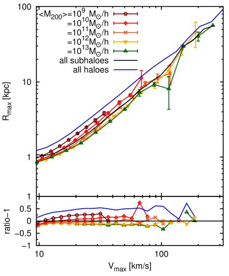
Figure 13: The $V_{max}-R_{max}$ diagram for subhaloes and haloes. Upper panel: the relation between the maximum circular velocity and the radius at which it is attained for subhaloes found in hosts of various masses (solid lines with symbols and error bars). The solid black line shows this relation for all subhaloes in the simulation, while the solid black line illustrates this relation for field haloes. Lower panel: the ratios of the different samples with respect to the ’all subhaloes’ sample.

A fundamental structural property of subhaloes is the relation between the maximum circular velocity, $V_{max}$, and the radius corresponding to this maximum, $R_{max}$. For DM dominated objects like spheroidal dwarf galaxies, the kinematics of the stellar component can be related to the underlying DM density profile via the ${V_{max}-R_{max}}$ relation, which is the basis of numerous cosmological studies based on the stellar kinematics of Local Group dwarf galaxies (see e.g. Boylan-Kolchin, Bullock & Kaplinghat, 2011, 2012; Sawala et al., 2013, 2016, 2015, 2014; Wang et al., 2012; Cautun et al., 2014a; Di Cintio et al., 2013; Zolotov et al., 2012; Arraki et al., 2014). While it is not our intention to have a detailed study of the $V_{max}-R_{max}$ relation, we would like to add to the discussion by presenting an interesting finding. Namely, in Fig. 13 we plot the $V_{max}-R_{max}$ diagram for both haloes and subhaloes. The lines with error bars mark the mean relation for subhaloes found in hosts of different masses. The solid black line corresponds to the values obtained by considering all resolved subhaloes in our simulation, while the solid blue curve indicates the same relation computed for field, isolated haloes. The mean $R_{max}$ value at fixed $V_{max}$ is a crude measure of central (sub)halo densities, as objects with the same $V_{max}$, but larger (smaller) $R_{max}$ values are characterised by lower (higher) central densities. Fig. 13 shows that at fixed $V_{max}$, the mean $R_{max}$ values for haloes are $50\%$ higher than for subhaloes. This can be easily seen as the blue solid line in the bottom panel of the figure. This behaviour reflects a well known fact, that subhaloes tend to have more concentrated density profiles due to the effects of tidal stripping, which become significant once the subhaloes fell into their respective hosts (see e.g. Moore et al., 1999; Diemand, Kuhlen & Madau, 2007; Springel et al., 2008) The tidal forces truncate a subhalo’s density profile by removing the mass that is only weakly gravitationally bound to the object. Since field haloes are rarely the subject of severe tidal forces, no such stripping takes place. An even more interesting find is the systematic difference, at fixed $V_{max}$, between the mean $R_{max}$ values characterizing subhaloes found in host haloes of different masses. Hence, satellites with the same $V_{max}$ values tend to have systematically higher $R_{max}$ values when found in central haloes of lower mass.

5 Conclusions

Since the establishment in the late 80s and 90s of the CDM model as the standard model for cosmic structure formation, it has become a subject of extensive tests and scrutiny. To understand the process of galaxy formation and evolution in a hierarchical $\Lambda{\rm CDM}$ cosmology, we need detailed knowledge of a multitude of physical processes that act over an overwhelming range of scales. The formation and dynamical evolution of haloes and subhaloes, from tiny DM specks of Earth mass to the most massive gravitationally bound objects, together with highly non-linear and complicated baryonic processes set the framework in which galaxies live and evolve in our Universe. The constant development of observational techniques is calling for an improvement in our theoretical modelling and understanding of the crucial phenomena involved. For this reason, we need simulations with ever growing resolution. However, we also need to model large enough cosmic volumes to obtain reliable statistics for various objects, from dwarf to giant galaxies. This is where simulations like the Copernicus Complexio play a pivotal role, since they have both a very high resolution and a large cosmological volume. In this paper we have introduced a new simulation, the coco, that can reliable resolve all substructure down to a $V_{max}\sim 10$ kms^-1 in a cosmological relevant volume of $\sim 2.2\times 10^{4}h^{-3}\,{\rm Mpc}^{3}$. This simulation is the first of its kind and is meant to be part of a whole series of intermediate zoom-in runs implementing both more $\Lambda{\rm CDM}$ cosmic volumes but also alternative DM physics like Warm or Self-Interacting DM models (see also Bose et al., 2016).

The following is a summary of our main results:

• The FOF mass function matches the ST and Reed formulas over seven orders of magnitude in halo mass at $z=0$. However, for the intermediate redshift range of $2<z<0.5$, the ST formula tends to over-predict the number of collapsed objects.

• We have observed a departure of the $c-M_{200}$ relation from a single power-law at lower halo masses, in agreement with the results of Sánchez-Conde & Prada (2014). We give a best fit to the coco data that reliably describes the concentration-mass relation of relaxed haloes over six decades in halo mass $10^{8}\leq M_{200}/(h^{-1}{\rm M}_{\odot})\leq 10^{14}$.

• We have probed the redshift evolution of the $c-M_{200}$ relation in the redshift interval, $9\leq z\leq 0$, to find that it is monotonic for small halo masses.

• The hierarchical nature of halo formation processes is confirmed for seven orders of magnitude in mass. The object-to-object scatter of the halo formation time depends on halo mass, with lower mass haloes showing a significantly larger scatter. This most likely is a manifestation of halo assembly bias, reflecting the multitude of environments in which low mass haloes are formed and evolve.

• We have confirmed the power-law character of the subhalo mass function, $\overline{N}(>\mu)\propto\mu^{-s}$, down to a rescaled subhalo mass, $\mu=10^{-6}$. For our best resolved hosts, with median halo mass, $\langle M_{200}\rangle=10^{13}h^{-1}{\rm M}_{\odot}$, we find a power-law exponent, $s=0.95\pm 0.01$.

• We find that the power-law exponent, $s$, depends on the host halo mass. It varies from $s=0.97\pm 0.02$ for cluster mass haloes (Gao et al., 2012) to $s=0.92\pm 0.02$ for $10^{10}h^{-1}{\rm M}_{\odot}$ haloes.

• Our data confirms over a wider dynamical range in subhalo sizes and down to lower host masses that the mean subhalo abundance, $\overline{N}(>\nu)$, when expressed in terms of $\nu=V_{max}/V_{200}$, is to a very good approximation independent of host halo mass. The best-fitting results for $\overline{N}(>\nu)$, which were proposed by Cautun et al. (2014b), match our data down to our resolution limit.

• The radial distribution of galactic subhaloes is nearly independent of subhalo mass, albeit with a very weak trend. Due to a large host-to-host scatter, this trend becomes visible only once we average over a substantial number of host haloes. In addition, the radial distribution of subhaloes is nearly universal for hosts differing by three orders of magnitude in halo mass.

• Finally, we have found that at fixed $V_{max}$ the mean $R_{max}$ values of subhaloes depend on the host halo mass, with lower mass hosts having subhaloes with higher $R_{max}$ values. This most likely reflects that at fixed subhalo size the tidal stripping processes are more efficient in more massive hosts.

The current and future runs of the coco suite will allow us to further test models of cosmic structure formation, including the development of semi-analytical galaxy formation models into the regime of low mass (sub)halo (hence also low galaxy luminosity) (for more details see Guo et al., 2015). This new satellite galaxy catalogue build on the base on coco was alreay used for stringent statistical study of the prevalence of rare plannar sattellite configurations in the $\Lambda{\rm CDM}$ (Cautun et al., 2015). Moreover, our new set of simulations will allow for a better statistical study of radio-flux anomalies and lensing arc-distortions, the low-luminosity galaxy population, reionisation treatment in semi-analytical models and effects of the large-scale structures (Cosmic Web) on (sub)halo and galaxy properties and distributions. As these projects are currently work in progress, with the publication of this paper we also intend to make publicly available, in a short time, all relevant coco halo and subhalo data bases accompanied by semi-analytical galaxy catalogues. In doing so, our hope and intention is to allow other researchers to use the coco data for their own research projects.

Appendix A Numerical convergence and resolution test

Here we assess a conservative limit for the mass and maximum circular velocity of the haloes and subhaloes that were resolved reliably in our simulations. This is necessary since haloes and especially subhaloes that are resolved at low resolution are subject to many numerical artefacts that can alter their inner properties like density and circular velocity profiles, leading to unphysical results. In the following, we present two tests for determining the resolution limit of our numerical experiment.

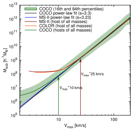
Figure 14: A comparison of the $V_{max}-M_{sub}$ relation for subhaloes found in hosts of all masses at redshift, $z=0$. The coco, color and ms-II lines depict the median relation found by binning the subhaloes according to their $V_{max}$ values. The shaded green region illustrates the 16th to 84th percentiles around the median for the coco sample. We also show the best fit power laws (Eq. 15) to the coco and ms-II data.

The first test investigates the relationship between the mass, $M_{sub}$, and the maximum circular velocity, $V_{max}$, of subhaloes. Following Boylan-Kolchin et al. (2010), we fit the relation with the power-law

$$M_{sub}=6\times 10^{10}\left({V_{max}}\over{100\textrm{km s}^{-1}}\right)^{s}\,h^{-1}{\rm M}_{\odot}\,.$$ (15)

Boylan-Kolchin et al. have found that such a power law, with $s=3.23$, provides a very good description of the ms-II data down to $V_{max}=25$ km s^-1. Below this value, the $V_{max}-M_{sub}$ relation deviates from the power law fit suggesting that subhaloes with lower $V_{max}$ values are affected by numerical resolution effects. The same power law, albeit with a slightly steeper scaling exponent, $s=3.3$, gives a very good fit to the coco data too, as shown in Fig. 14. The coco subhaloes follow the power law relation down to a much smaller $V_{max}$ values of $\sim 10$ km s^-1 ($M_{sub}\sim 5\times 10^{7}h^{-1}{\rm M}_{\odot}$). Fig. 14 also shows that that there is a very good convergence between the color and the coco runs, with color having a resolution limit of $V_{max}=25$ km s^-1. color has the same behaviour as ms-II since both simulations have the same particle mass and force resolution.

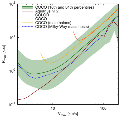
Figure 15: A comparison of the $V_{max}-R_{max}$ relation for haloes versus that for subhaloes. The solid yellow and orange lines show the relation for main haloes in the coco and color samples. The remaining lines show the $V_{max}-R_{max}$ relation for subhaloes identified in all the coco hosts (green solid line); in Milky-Way mass hosts ( blue dashed line;see §4.3); and in the aquarius level 2 hosts (solid brown line). The green shaded region gives the 16th to 84th percentiles for the full sample of coco subhaloes.

In the second test we compare the $V_{max}-R_{max}$ relation of subhaloes with the same relation for haloes (see Fig. 15). We find that both for haloes and subhaloes, the median $V_{max}-R_{max}$ relation shows an upturn indicative of numerical resolution effects at $V_{max}=10$ and 25 km s^-1 for coco and color, respectively. Thus, the two $V_{max}$ thresholds give a good conservative estimate for the resolution limit of our two simulations.

References

- Abel, Hahn & Kaehler (2012) Abel T., Hahn O., Kaehler R., 2012, MNRAS, 427, 61
- Alimi et al. (2012) Alimi J.-M. et al., 2012, in Proceedings of the International Conference on High Performance Computing, Networking, Storage and Analysis, SC ’12, IEEE Computer Society Press, Los Alamitos, CA, USA, pp. 73:1–73:11
- Anderhalden & Diemand (2013) Anderhalden D., Diemand J., 2013, J. Cosmology Astropart. Phys, 4, 9
- Anderson et al. (2012) Anderson L. et al., 2012, MNRAS, 427, 3435
- Angulo et al. (2012) Angulo R. E., Springel V., White S. D. M., Jenkins A., Baugh C. M., Frenk C. S., 2012, MNRAS, 426, 2046
- Aragón-Calvo, van de Weygaert & Jones (2010) Aragón-Calvo M. A., van de Weygaert R., Jones B. J. T., 2010, MNRAS, 408, 2163
- Arraki et al. (2014) Arraki K. S., Klypin A., More S., Trujillo-Gomez S., 2014, MNRAS, 438, 1466
- Bardeen et al. (1986) Bardeen J. M., Bond J. R., Kaiser N., Szalay A. S., 1986, ApJ, 304, 15
- Belokurov et al. (2014) Belokurov V., Irwin M. J., Koposov S. E., Evans N. W., Gonzalez-Solares E., Metcalfe N., Shanks T., 2014, MNRAS, 441, 2124
- Belokurov et al. (2006) Belokurov V. et al., 2006, ApJ, 642, L137
- Belokurov et al. (2007) Belokurov V. et al., 2007, ApJ, 654, 897
- Benson et al. (2003) Benson A. J., Bower R. G., Frenk C. S., Lacey C. G., Baugh C. M., Cole S., 2003, ApJ, 599, 38
- Bergström, Ullio & Buckley (1998) Bergström L., Ullio P., Buckley J. H., 1998, Astroparticle Physics, 9, 137
- Bond, Kofman & Pogosyan (1996) Bond J. R., Kofman L., Pogosyan D., 1996, Nature, 380, 603
- Bose et al. (2016) Bose S., Hellwing W. A., Frenk C. S., Jenkins A., Lovell M. R., Helly J. C., Li B., 2016, MNRAS, 455, 318
- Bower et al. (2006) Bower R. G., Benson A. J., Malbon R., Helly J. C., Frenk C. S., Baugh C. M., Cole S., Lacey C. G., 2006, MNRAS, 370, 645
- Boylan-Kolchin (2014) Boylan-Kolchin M., 2014, Nature, 509, 170
- Boylan-Kolchin, Bullock & Kaplinghat (2011) Boylan-Kolchin M., Bullock J. S., Kaplinghat M., 2011, MNRAS, 415, L40
- Boylan-Kolchin, Bullock & Kaplinghat (2012) Boylan-Kolchin M., Bullock J. S., Kaplinghat M., 2012, MNRAS, 422, 1203
- Boylan-Kolchin et al. (2010) Boylan-Kolchin M., Springel V., White S. D. M., Jenkins A., 2010, MNRAS, 406, 896
- Boylan-Kolchin et al. (2009) Boylan-Kolchin M., Springel V., White S. D. M., Jenkins A., Lemson G., 2009, MNRAS, 398, 1150
- Brook & Di Cintio (2015) Brook C. B., Di Cintio A., 2015, MNRAS, 450, 3920
- Cautun et al. (2015) Cautun M., Bose S., Frenk C. S., Guo Q., Han J., Hellwing W. A., Sawala T., Wang W., 2015, MNRAS, 452, 3838
- Cautun et al. (2014a) Cautun M., Frenk C. S., van de Weygaert R., Hellwing W. A., Jones B. J. T., 2014a, MNRAS, 445, 2049
- Cautun et al. (2014b) Cautun M., Hellwing W. A., van de Weygaert R., Frenk C. S., Jones B. J. T., Sawala T., 2014b, MNRAS, 445, 1820
- Cautun et al. (2014c) Cautun M., van de Weygaert R., Jones B. J. T., Frenk C. S., 2014c, MNRAS, 441, 2923
- Cole et al. (1994) Cole S., Aragon-Salamanca A., Frenk C. S., Navarro J. F., Zepf S. E., 1994, MNRAS, 271, 781
- Cole & Kaiser (1989) Cole S., Kaiser N., 1989, MNRAS, 237, 1127
- Cole & Lacey (1996) Cole S., Lacey C., 1996, MNRAS, 281, 716
- Cole et al. (2000) Cole S., Lacey C. G., Baugh C. M., Frenk C. S., 2000, MNRAS, 319, 168
- Cole et al. (2005) Cole S. et al., 2005, MNRAS, 362, 505
- Correa et al. (2015a) Correa C. A., Wyithe J. S. B., Schaye J., Duffy A. R., 2015a, MNRAS, 450, 1514
- Correa et al. (2015b) Correa C. A., Wyithe J. S. B., Schaye J., Duffy A. R., 2015b, MNRAS, 450, 1521
- Correa et al. (2015c) Correa C. A., Wyithe J. S. B., Schaye J., Duffy A. R., 2015c, MNRAS, 452, 1217
- Crain et al. (2009) Crain R. A. et al., 2009, MNRAS, 399, 1773
- Croton, Gao & White (2007) Croton D. J., Gao L., White S. D. M., 2007, MNRAS, 374, 1303
- Davis et al. (1985) Davis M., Efstathiou G., Frenk C. S., White S. D. M., 1985, ApJ, 292, 371
- de la Torre et al. (2013) de la Torre S. et al., 2013, A&A, 557, A54
- De Lucia & Blaizot (2007) De Lucia G., Blaizot J., 2007, MNRAS, 375, 2
- De Lucia et al. (2004) De Lucia G., Kauffmann G., Springel V., White S. D. M., Lanzoni B., Stoehr F., Tormen G., Yoshida N., 2004, MNRAS, 348, 333
- Di Cintio et al. (2013) Di Cintio A., Knebe A., Libeskind N. I., Brook C., Yepes G., Gottlöber S., Hoffman Y., 2013, MNRAS, 431, 1220
- Diemand, Kuhlen & Madau (2007) Diemand J., Kuhlen M., Madau P., 2007, ApJ, 657, 262
- Diemand, Moore & Stadel (2004) Diemand J., Moore B., Stadel J., 2004, MNRAS, 352, 535
- Diemand, Moore & Stadel (2005) Diemand J., Moore B., Stadel J., 2005, Nature, 433, 389
- Diemer & Kravtsov (2015) Diemer B., Kravtsov A. V., 2015, ApJ, 799, 108
- Driver et al. (2009) Driver S. P. et al., 2009, Astronomy and Geophysics, 50, 12
- Dutton & Macciò (2014) Dutton A. A., Macciò A. V., 2014, MNRAS, 441, 3359
- Einasto (1965) Einasto J., 1965, Trudy Astrofizicheskogo Instituta Alma-Ata, 5, 87
- Eisenstein et al. (2005) Eisenstein D. J. et al., 2005, ApJ, 633, 560
- Falck et al. (2014) Falck B., Koyama K., Zhao G.-b., Li B., 2014, J. Cosmology Astropart. Phys, 7, 58
- Fosalba et al. (2015) Fosalba P., Crocce M., Gaztañaga E., Castander F. J., 2015, MNRAS, 448, 2987
- Frenk et al. (1996) Frenk C. S., Evrard A. E., White S. D. M., Summers F. J., 1996, ApJ, 472, 460
- Frenk & White (2012) Frenk C. S., White S. D. M., 2012, Annalen der Physik, 524, 507
- Frenk et al. (1988) Frenk C. S., White S. D. M., Davis M., Efstathiou G., 1988, ApJ, 327, 507
- Frenk et al. (1985) Frenk C. S., White S. D. M., Efstathiou G., Davis M., 1985, Nature, 317, 595
- Gao et al. (2008) Gao L., Navarro J. F., Cole S., Frenk C. S., White S. D. M., Springel V., Jenkins A., Neto A. F., 2008, MNRAS, 387, 536
- Gao et al. (2012) Gao L., Navarro J. F., Frenk C. S., Jenkins A., Springel V., White S. D. M., 2012, MNRAS, 425, 2169
- Gao & White (2007) Gao L., White S. D. M., 2007, MNRAS, 377, L5
- Gao et al. (2004) Gao L., White S. D. M., Jenkins A., Stoehr F., Springel V., 2004, MNRAS, 355, 819
- Garrison-Kimmel et al. (2014a) Garrison-Kimmel S., Boylan-Kolchin M., Bullock J. S., Kirby E. N., 2014a, MNRAS, 444, 222
- Garrison-Kimmel et al. (2014b) Garrison-Kimmel S., Boylan-Kolchin M., Bullock J. S., Lee K., 2014b, MNRAS, 438, 2578
- Gondolo & Silk (1999) Gondolo P., Silk J., 1999, Physical Review Letters, 83, 1719
- Gottloeber, Hoffman & Yepes (2010) Gottloeber S., Hoffman Y., Yepes G., 2010, ArXiv e-prints
- Gottloeber et al. (2006) Gottloeber S., Yepes G., Wagner C., Sevilla R., 2006, ArXiv Astrophysics e-prints
- Green, Hofmann & Schwarz (2004) Green A. M., Hofmann S., Schwarz D. J., 2004, MNRAS, 353, L23
- Guo et al. (2015) Guo Q., Cooper A. P., Frenk C., Helly J., Hellwing W. A., 2015, MNRAS, 454, 550
- Guo et al. (2013) Guo Q., White S., Angulo R. E., Henriques B., Lemson G., Boylan-Kolchin M., Thomas P., Short C., 2013, MNRAS, 428, 1351
- Guo et al. (2010) Guo Q., White S., Li C., Boylan-Kolchin M., 2010, MNRAS, 404, 1111
- Hahn, Abel & Kaehler (2013) Hahn O., Abel T., Kaehler R., 2013, MNRAS, 434, 1171
- Harrison (1970) Harrison E. R., 1970, Phys. Rev. D, 1, 2726
- Heitmann et al. (2010) Heitmann K., White M., Wagner C., Habib S., Higdon D., 2010, ApJ, 715, 104
- Helly et al. (2003) Helly J. C., Cole S., Frenk C. S., Baugh C. M., Benson A., Lacey C., 2003, MNRAS, 338, 903
- Hinshaw et al. (2013) Hinshaw G. et al., 2013, ApJS, 208, 19
- Hopkins et al. (2010) Hopkins P. F. et al., 2010, ApJ, 715, 202
- Ibata et al. (2013) Ibata R. A. et al., 2013, Nature, 493, 62
- Ishiyama et al. (2013) Ishiyama T. et al., 2013, ApJ, 767, 146
- Jenkins (2010) Jenkins A., 2010, MNRAS, 403, 1859
- Jenkins (2013) Jenkins A., 2013, MNRAS, 434, 2094
- Jenkins et al. (2001) Jenkins A., Frenk C. S., White S. D. M., Colberg J. M., Cole S., Evrard A. E., Couchman H. M. P., Yoshida N., 2001, MNRAS, 321, 372
- Jiang et al. (2014) Jiang L., Helly J. C., Cole S., Frenk C. S., 2014, MNRAS, 440, 2115
- Katz & White (1993) Katz N., White S. D. M., 1993, ApJ, 412, 455
- Kauffmann & White (1993) Kauffmann G., White S. D. M., 1993, MNRAS, 261, 921
- Kauffmann, White & Guiderdoni (1993) Kauffmann G., White S. D. M., Guiderdoni B., 1993, MNRAS, 264, 201
- Kim et al. (2009) Kim J., Park C., Gott, III J. R., Dubinski J., 2009, ApJ, 701, 1547
- Kim et al. (2011) Kim J., Park C., Rossi G., Lee S. M., Gott, III J. R., 2011, Journal of Korean Astronomical Society, 44, 217
- Klypin et al. (1999a) Klypin A., Gottlöber S., Kravtsov A. V., Khokhlov A. M., 1999a, ApJ, 516, 530
- Klypin et al. (1999b) Klypin A., Kravtsov A. V., Valenzuela O., Prada F., 1999b, ApJ, 522, 82
- Klypin, Trujillo-Gomez & Primack (2011) Klypin A. A., Trujillo-Gomez S., Primack J., 2011, ApJ, 740, 102
- Knollmann & Knebe (2009) Knollmann S. R., Knebe A., 2009, ApJS, 182, 608
- Kochanek & Dalal (2004) Kochanek C. S., Dalal N., 2004, ApJ, 610, 69
- Komatsu et al. (2011) Komatsu E. et al., 2011, ApJS, 192, 18
- Koposov et al. (2008) Koposov S. et al., 2008, ApJ, 686, 279
- Kravtsov et al. (2004) Kravtsov A. V., Berlind A. A., Wechsler R. H., Klypin A. A., Gottlöber S., Allgood B., Primack J. R., 2004, ApJ, 609, 35
- Lacey & Cole (1993) Lacey C., Cole S., 1993, MNRAS, 262, 627
- Lavalle et al. (2008) Lavalle J., Yuan Q., Maurin D., Bi X.-J., 2008, A&A, 479, 427
- Li, Mo & Gao (2008) Li Y., Mo H. J., Gao L., 2008, MNRAS, 389, 1419
- Ludlow et al. (2014) Ludlow A. D., Navarro J. F., Angulo R. E., Boylan-Kolchin M., Springel V., Frenk C., White S. D. M., 2014, MNRAS, 441, 378
- Ludlow et al. (2013) Ludlow A. D. et al., 2013, MNRAS, 432, 1103
- Ludlow et al. (2010) Ludlow A. D., Navarro J. F., Springel V., Vogelsberger M., Wang J., White S. D. M., Jenkins A., Frenk C. S., 2010, MNRAS, 406, 137
- Mao & Schneider (1998) Mao S., Schneider P., 1998, MNRAS, 295, 587
- McConnachie (2012) McConnachie A. W., 2012, AJ, 144, 4
- McConnachie & Irwin (2006) McConnachie A. W., Irwin M. J., 2006, MNRAS, 365, 902
- McConnachie et al. (2009) McConnachie A. W. et al., 2009, Nature, 461, 66
- Merson et al. (2013) Merson A. I. et al., 2013, MNRAS, 429, 556
- Metcalf & Madau (2001) Metcalf R. B., Madau P., 2001, ApJ, 563, 9
- Metcalf & Zhao (2002) Metcalf R. B., Zhao H., 2002, ApJ, 567, L5
- Metuki et al. (2015) Metuki O., Libeskind N. I., Hoffman Y., Crain R. A., Theuns T., 2015, MNRAS, 446, 1458
- Metz, Kroupa & Libeskind (2008) Metz M., Kroupa P., Libeskind N. I., 2008, ApJ, 680, 287
- Moore et al. (1999) Moore B., Ghigna S., Governato F., Lake G., Quinn T., Stadel J., Tozzi P., 1999, ApJ, 524, L19
- Nagai & Kravtsov (2005) Nagai D., Kravtsov A. V., 2005, ApJ, 618, 557
- Navarro, Frenk & White (1996) Navarro J. F., Frenk C. S., White S. D. M., 1996, ApJ, 462, 563
- Navarro, Frenk & White (1997) Navarro J. F., Frenk C. S., White S. D. M., 1997, ApJ, 490, 493
- Navarro et al. (2004) Navarro J. F. et al., 2004, MNRAS, 349, 1039
- Neto et al. (2007) Neto A. F. et al., 2007, MNRAS, 381, 1450
- Nuza et al. (2014) Nuza S. E., Kitaura F.-S., Heß S., Libeskind N. I., Müller V., 2014, MNRAS, 445, 988
- Oñorbe et al. (2015) Oñorbe J., Boylan-Kolchin M., Bullock J. S., Hopkins P. F., Kereš D., Faucher-Giguère C.-A., Quataert E., Murray N., 2015, MNRAS, 454, 2092
- Oñorbe et al. (2014) Oñorbe J., Garrison-Kimmel S., Maller A. H., Bullock J. S., Rocha M., Hahn O., 2014, MNRAS, 437, 1894
- Pawlowski & Kroupa (2013) Pawlowski M. S., Kroupa P., 2013, MNRAS, 435, 2116
- Peebles (1982) Peebles P. J. E., 1982, ApJ, 263, L1
- Percival et al. (2010) Percival W. J. et al., 2010, MNRAS, 401, 2148
- Planck Collaboration et al. (2014) Planck Collaboration et al., 2014, A&A, 571, A16
- Planck Collaboration et al. (2015) Planck Collaboration et al., 2015, ArXiv e-prints
- Pontzen & Governato (2012) Pontzen A., Governato F., 2012, MNRAS, 421, 3464
- Power & Knebe (2006) Power C., Knebe A., 2006, MNRAS, 370, 691
- Power, Knebe & Knollmann (2012) Power C., Knebe A., Knollmann S. R., 2012, MNRAS, 419, 1576
- Power et al. (2003) Power C., Navarro J. F., Jenkins A., Frenk C. S., White S. D. M., Springel V., Stadel J., Quinn T., 2003, MNRAS, 338, 14
- Prada et al. (2012) Prada F., Klypin A. A., Cuesta A. J., Betancort-Rijo J. E., Primack J., 2012, MNRAS, 423, 3018
- Prada et al. (2006) Prada F., Klypin A. A., Simonneau E., Betancort-Rijo J., Patiri S., Gottlöber S., Sanchez-Conde M. A., 2006, ApJ, 645, 1001
- Press & Schechter (1974) Press W. H., Schechter P., 1974, Astrophys. J., 187, 425
- Prunet et al. (2008) Prunet S., Pichon C., Aubert D., Pogosyan D., Teyssier R., Gottloeber S., 2008, ApJS, 178, 179
- Rasera et al. (2014) Rasera Y., Corasaniti P.-S., Alimi J.-M., Bouillot V., Reverdy V., Balmès I., 2014, MNRAS, 440, 1420
- Reed et al. (2007) Reed D. S., Bower R., Frenk C. S., Jenkins A., Theuns T., 2007, MNRAS, 374, 2
- Roukema et al. (1997) Roukema B. F., Quinn P. J., Peterson B. A., Rocca-Volmerange B., 1997, MNRAS, 292, 835
- Sánchez-Conde & Prada (2014) Sánchez-Conde M. A., Prada F., 2014, MNRAS, 442, 2271
- Sawala et al. (2013) Sawala T., Frenk C. S., Crain R. A., Jenkins A., Schaye J., Theuns T., Zavala J., 2013, MNRAS, 431, 1366
- Sawala et al. (2014) Sawala T. et al., 2014, ArXiv e-prints
- Sawala et al. (2015) Sawala T. et al., 2015, MNRAS, 448, 2941
- Sawala et al. (2016) Sawala T. et al., 2016, MNRAS, 456, 85
- Schaye et al. (2015) Schaye J. et al., 2015, MNRAS, 446, 521
- Shandarin & Zeldovich (1989) Shandarin S. F., Zeldovich Y. B., 1989, Reviews of Modern Physics, 61, 185
- Shaw et al. (2006) Shaw L. D., Weller J., Ostriker J. P., Bode P., 2006, ApJ, 646, 815
- Sheth & Tormen (2002) Sheth R. K., Tormen G., 2002, MNRAS, 329, 61
- Sheth & van de Weygaert (2004) Sheth R. K., van de Weygaert R., 2004, MNRAS, 350, 517
- Springel (2005) Springel V., 2005, MNRAS, 364, 1105
- Springel, Frenk & White (2006) Springel V., Frenk C. S., White S. D. M., 2006, Nature, 440, 1137
- Springel et al. (2008) Springel V. et al., 2008, MNRAS, 391, 1685
- Springel et al. (2005) Springel V. et al., 2005, Nature, 435, 629
- Springel et al. (2001) Springel V., White S. D. M., Tormen G., Kauffmann G., 2001, MNRAS, 328, 726
- Teyssier et al. (2009) Teyssier R. et al., 2009, A&A, 497, 335
- Tinker et al. (2008) Tinker J., Kravtsov A. V., Klypin A., Abazajian K., Warren M., Yepes G., Gottlöber S., Holz D. E., 2008, ApJ, 688, 709
- Vogelsberger et al. (2014) Vogelsberger M. et al., 2014, MNRAS, 444, 1518
- Wang, Frenk & Cooper (2013) Wang J., Frenk C. S., Cooper A. P., 2013, MNRAS, 429, 1502
- Wang et al. (2012) Wang J., Frenk C. S., Navarro J. F., Gao L., Sawala T., 2012, MNRAS, 424, 2715
- Warren et al. (2006) Warren M. S., Abazajian K., Holz D. E., Teodoro L., 2006, ApJ, 646, 881
- Watson et al. (2014) Watson W. A. et al., 2014, MNRAS, 438, 412
- Wechsler et al. (2002) Wechsler R. H., Bullock J. S., Primack J. R., Kravtsov A. V., Dekel A., 2002, ApJ, 568, 52
- White & Frenk (1991) White S. D. M., Frenk C. S., 1991, ApJ, 379, 52
- White & Rees (1978) White S. D. M., Rees M. J., 1978, MNRAS, 183, 341
- Xu et al. (2015) Xu D., Sluse D., Gao L., Wang J., Frenk C., Mao S., Schneider P., Springel V., 2015, MNRAS, 447, 3189
- Yang, Mo & van den Bosch (2003) Yang X., Mo H. J., van den Bosch F. C., 2003, MNRAS, 339, 1057
- Zeldovich (1972) Zeldovich Y. B., 1972, MNRAS, 160, 1P
- Zolotov et al. (2012) Zolotov A. et al., 2012, ApJ, 761, 71