New summation inequalities and their applications to discrete-time delay systems

Abstract

This paper provides new summation inequalities in both single and double forms to be used in stability analysis of discrete-time systems with time-varying delays. The potential capability of the newly derived inequalities is demonstrated by establishing less conservative stability conditions for a class of linear discrete-time systems with an interval time-varying delay in the framework of linear matrix inequalities. The effectiveness and least conservativeness of the derived stability conditions are shown by academic and practical examples.

I Introduction

It is well known that time-delay frequently occurs in practical systems and usually is a source of bad performance, oscillations or instability [1, 2]. Therefore, the problem of stability analysis and applications to control of time-delay systems are essential and of great importance for both theoretical and practical reasons which have attracted considerable attention, see, for example [3, 4, 5, 6, 7, 8, 9, 10] and the references therein.

Among existing works which concern with stability of linear time-delay systems, the Lyapunov-Krasovskii functional (LKF) method plays an essential role in deriving efficient stability conditions. Based on a priori construction of a Lyapunov-Krasovskii functional combining with some bounding techniques [4, 7, 10, 11, 12], improved delay-dependent stability conditions for continuous/discrete time-delay systems were derived in terms of tractable linear matrix inequalities [7, 10, 12, 13]. However, the design of such Lyapunov-Krasovskii functional and especially the techniques used in bounding the derivative or difference of constructed Lyapunov-Krasovskii functional usually produce an undesirable conservatism in stability conditions. Therefore, aiming at reducing conservativeness of stability conditions, it is relevant and important to improve some fundamental inequalities to be used in establishing such stability criteria [10, 14].

Note that, most of the aforementioned works have been devoted to continuous-time systems. Besides, the problem of stability analysis and control of discrete-time systems with time-varying delay is very relevant and therefore it should be receiving a greater focus due to the following practical reasons. Firstly, with the rapid development of computer-based computational techniques, discrete-time systems are more suitable for computer simulation, experiment and computation. Secondly, many practical systems are in the form of nonlinear and/or non-autonomous continuous-time systems with time-varying delays. A discretization from continuous-time systems leads to discrete-time systems described by difference equations which inherit the similar dynamical behavior of the continuous ones[15]. In addition, the investigation of stability and control of discrete-time systems requires specific and quite different tools from the continuous ones. Thus, stability analysis and control of discrete-time delay systems have received considerable attention in recent years [16, 17, 18, 19, 20, 21, 22, 23, 24]. Most recently, novel summation inequalities were derived [25, 26] by extending the Wirtinger-based integral inequality [7]. These summation inequalities provide a powerful tool to derive less conservative stability conditions for discrete-time systems with interval time-varying delay in the framework of tractable linear matrix inequalities.

In this paper, new summation inequalities which provide an efficient tool for stability analysis of discrete-time systems with time-varying delay are fisrt derived. Inspired by the approaches proposed in [10, 14] for the continuous-time systems, new summation inequalities in both single and double forms are derived by refining the discrete Jensen inequalities. It is worth noting that the obtained results in this paper theoretically encompass the summation inequalities proposed in [26, 25]. Furthermore, unlike [26, 25], we prove that the proposed inequalities do not depend on the choice of first-order approximation sequences. By employing these new inequalities, a suitable Lyapunov-Krasovskii functional is constructed and less conservative stability conditions are derived for a class of discrete-time systems with interval time-varying delay. To illustrate the effectiveness of the proposed stability conditions, an academic example and a practical satellite control system are provided. These examples show that our stability conditions provide significant improvement over existing works in the literature.

The paper is organized as follows. Section II presents some preliminary results. New summation inequalities and their applications to stability analysis of a class of discrete-time systems with interval time-varying delay are presented in Section III and Section IV, respectively. Numerical examples to demonstrate the effectiveness of the obtained results are also given in Section IV.

II Preliminaries

Notations: Throughout this paper, we denote $\mathbb{Z}$ and $\mathbb{Z}^{+}$ the set of integers and positive integers, respectively, $\mathbb{R}^{n}$ the $n$-dimensional Euclidean space with vector norm $\|.\|$, $\mathbb{R}^{n\times m}$ the set of $n\times m$ real matrices. For matrices $A,B\in\mathbb{R}^{n\times m}$, $\mathrm{col}\{A,B\}$ and $\mathrm{diag}\{A,B\}$ denote the block matrix $\begin{bmatrix}A\\ B\end{bmatrix}$ and $\begin{bmatrix}A&0\\ 0&B\end{bmatrix}$, respectively. A matrix $P\in\mathbb{R}^{n\times n}$ is positive (negative) definite, write $P>0$ ($P<0$) if $x^{T}Px>0$ ($x^{T}Px<0$) for all $x\in\mathbb{R}^{n}$, $x\neq 0$. We let $\mathbb{S}^{+}_{n}$ denote the set of symmetric positive definite matrices. For any $A\in\mathbb{R}^{n\times n}$, $\mathtt{He}(A)$ stands for $A+A^{T}$. For $a,b\in\mathbb{Z}$, $a\leq b$, $\mathbb{Z}[a,b]$ denotes the set of integers between $a$ and $b$. For a sequence $u:\mathbb{Z}[a,b]\to\mathbb{R}^{n}$, we write $u_{k}=u(k)$, $k\in\mathbb{Z}[a,b]$, $\Delta$ denotes the forward difference operator, that means $\Delta u_{k}=u_{k+1}-u_{k}$. For any two sequences $u,v:\mathbb{Z}[a,b]\to\mathbb{R}^{n}$, it is obvious that $u_{k}\Delta v_{k}=\Delta(u_{k}v_{k})-v_{k+1}\Delta u_{k}$.

The following inequalities which are widely used in the literature can be easily derived by using Schur complement lemma.

Lemma 1:

(Jensen’s inequalities) For a given matrix $R\in\mathbb{S}^{+}_{n}$, integers $b>a$, any sequence $u:\mathbb{Z}[a,b]\to\mathbb{R}^{n}$, the following inequalities hold

$$\sum_{k=a}^{b}u^{T}_{k}Ru_{k}\geq\frac{1}{\ell}\big{(}\sum_{k=a}^{b}u_{k}\big{)}^{T}R\big{(}\sum_{k=a}^{b}u_{k}\big{)},$$ (1)

$$\sum_{k=a}^{b}\sum_{s=a}^{k}u_{s}^{T}Ru_{s}\geq\frac{2}{\ell(\ell+1)}\big{(}\sum_{k=a}^{b}\sum_{s=a}^{k}u_{s}\big{)}^{T}R\big{(}\sum_{k=a}^{b}\sum_{s=a}^{k}u_{s}\big{)},$$ (2)

where $\ell=b-a+1$ denotes the length of interval $[a,b]$ in $\mathbb{Z}$.

III New summation inequalities

In this section, new summation inequalities are derived by refining (1), (2). In the following, let us denote $J_{1}(u)$ and $J_{2}(u)$ as the gap of (1) and (2), respectively, that is the difference between the left-hand side and the right-hand side in (1) and (2). By refining (1) and (2), we aim to find new lower bounds for $J_{1}(u),J_{2}(u)$ other than zero.

Lemma 2:

For a given matrix $R\in\mathbb{S}^{+}_{n}$, integers $b>a$, any sequence $u:\mathbb{Z}[a,b]\to\mathbb{R}^{n}$, the following inequality holds

$$J_{1}(u)\geq\frac{3(\ell+1)}{\ell(\ell-1)}\zeta_{1}^{T}R\zeta_{1}+\frac{5(\ell+1)(\ell+2)^{2}}{\ell(\ell-1)(\ell^{2}+11)}\zeta_{2}^{T}R\zeta_{2}$$ (3)

where $\zeta_{1}=\upsilon_{1}-\frac{2}{\ell+1}\upsilon_{2}$, $\zeta_{2}=\upsilon_{1}-\frac{6}{\ell+1}\upsilon_{2}+\frac{12}{(\ell+1)(\ell+2)}\upsilon_{3}$ and $\upsilon_{1}=\sum\limits_{k=a}^{b}u_{k}$, $\upsilon_{2}=\sum\limits_{k=a}^{b}\sum\limits_{s=a}^{k}u_{s}$, $\upsilon_{3}=\sum\limits_{k=a}^{b}\sum\limits_{s=a}^{k}\sum\limits_{i=a}^{s}u_{i}$.

Proof: Note at first that if $\ell=1$ then $\zeta_{1}=\zeta_{2}=0$ and thus (3) holds. Now assume that $\ell>1$. We use the idea of bilevel optimization to get (3) by refining (1). To this, for a sequence $u:\mathbb{Z}[a,b]\to\mathbb{R}^{n}$, we define an approximation sequence $v:\mathbb{Z}[a,b]\to\mathbb{R}^{n}$ as follows

$$v_{k}=u_{k}-\frac{1}{\ell}\sum_{k=a}^{b}u_{k}+\alpha_{k}\chi_{1}+\beta_{k}\chi_{2}$$ (4)

where $\alpha_{k}$ and $\beta_{k}$ are two sequences of real numbers and $\chi_{1},\chi_{2}\in\mathbb{R}^{n}$ are constant vectors which will be defined later. From (4) we have

$$\sum_{k=a}^{b}v_{k}^{T}Rv_{k}= J_{1}(u)+2\chi_{1}^{T}R(\sum_{k=a}^{b}\alpha_{k}u_{k})+2\chi_{2}^{T}R(\sum_{k=a}^{b}\beta_{k}u_{k})$$ (5)

$$-\frac{2}{\ell}(\sum_{k=a}^{b}\alpha_{k})\chi_{1}^{T}R\upsilon_{1}-\frac{2}{\ell}(\sum_{k=a}^{b}\beta_{k})\chi_{2}^{T}R\upsilon_{1}$$

$$+(\sum_{k=a}^{b}\alpha_{k}^{2})\chi_{1}^{T}R\chi_{1}+(\sum_{k=a}^{b}\beta_{k}^{2})\chi_{2}^{T}R\chi_{2}$$

$$+2(\sum_{k=a}^{b}\alpha_{k}\beta_{k})\chi_{1}^{T}R\chi_{2}.$$

Let $\hat{u}_{k}=\sum\limits_{i=a}^{k-1}u_{i}$ for $k>a$, $\hat{u}_{k}=0$ for $k=a$, then $u_{k}=\Delta\hat{u}_{k}$ and, consequently, $\alpha_{k}u_{k}=\Delta(\alpha_{k}\hat{u}_{k})-\hat{u}_{k+1}\Delta\alpha_{k}$. Taking summation from $a$ to $b$ gives

$$\sum_{k=a}^{b}\alpha_{k}u_{k}=\alpha_{b+1}\sum_{k=a}^{b}u_{k}-\sum_{k=a}^{b}\hat{u}_{k+1}\Delta\alpha_{k}.$$ (6)

For any first-order sequence $\alpha_{k}$ which can be written as $\alpha_{k}=c_{0}(k-a)+c_{1}$, $c_{0}\neq 0$, we have

$$\alpha_{b+1}=c_{0}\ell+c_{1},\;\Delta\alpha_{k}=c_{0},\;\sum_{k=a}^{b}\alpha_{k}=c_{0}\frac{\ell(\ell-1)}{2}+c_{1}\ell.$$

This, in regard to (6), leads to

$$2\chi_{1}^{T}R(\sum_{k=a}^{b}\alpha_{k}u_{k})-\frac{2}{\ell}(\sum_{k=a}^{b}\alpha_{k})\chi_{1}^{T}R\upsilon_{1}=\alpha_{0}(\ell+1)\chi_{1}^{T}R\zeta_{1}.$$ (7)

Similar to (6) we have

$$\sum_{k=a}^{b}\beta_{k}u_{k}=\beta_{b+1}\sum_{k=a}^{b}u_{k}-\sum_{k=a}^{b}\hat{u}_{k+1}\Delta\beta_{k}.$$

At this time we define the sequence $\tilde{u}_{k}=\sum_{s=a}^{k}\hat{u}_{s}$ then $\hat{u}_{k+1}=\Delta\tilde{u}_{k}$ and thus

$$\hat{u}_{k+1}\Delta\beta_{k}=\Delta(\Delta\beta_{k}\tilde{u}_{k})-\tilde{u}_{k+1}\Delta^{2}\beta_{k}.$$

For convenience, we choose $\beta_{k}=(k-a)^{2}-\ell(k-a)+\frac{\ell^{2}-1}{6}$ then $\sum_{k=a}^{b}\beta_{k}=0$, $\beta_{b+1}=\frac{\ell^{2}-1}{6}$, $\Delta\beta_{b+1}=\ell+1$ and $\Delta^{2}(\beta_{k})=2$. Note also that

$$\sum_{k=a}^{b}\tilde{u}_{k+1}=\sum_{k=a}^{b}\sum_{s=a}^{k+1}\hat{u}_{i}=\sum_{k=a}^{b}\sum_{s=a+1}^{k+1}\hat{u}_{i}=\sum_{k=a}^{b}\sum_{s=a}^{k}\hat{u}_{i+1}=\upsilon_{3}.$$

Therefore

$$2\chi_{2}^{T}R(\sum_{k=a}^{b}\beta_{k}u_{k})-\frac{2}{\ell}(\sum_{k=a}^{b}\beta_{k})\chi_{2}^{T}R\upsilon_{1}=\frac{1}{3}\chi_{2}^{T}R\zeta_{3}$$ (8)

where $\zeta_{3}=(\ell^{2}-1)\upsilon_{1}-6(\ell+1)\upsilon_{2}+12\upsilon_{3}$.

On the other hand, from (4) and note that $\sum_{k=a}^{b}\beta_{k}=0$, we readily obtain $\sum_{k=a}^{b}v_{k}=(\sum_{k=a}^{b}\alpha_{k})\chi_{1}$. This, together with (5), (7) and (8), leads to

$$J_{1}(v)= J_{1}(u)+c_{0}(\ell+1)\chi_{1}^{T}R\zeta_{1}+\frac{1}{3}\chi_{2}^{T}R\zeta_{3}$$ (9)

$$+\Big{[}\sum_{k=a}^{b}\alpha_{k}^{2}-\frac{1}{\ell}\big{(}\sum_{k=a}^{b}\alpha_{k}\big{)}^{2}\Big{]}\chi_{1}^{T}R\chi_{1}$$

$$+(\sum_{k=a}^{b}\beta_{k}^{2})\chi_{2}^{T}R\chi_{2}+2(\sum_{k=a}^{b}\alpha_{k}\beta_{k})\chi_{1}^{T}R\chi_{2}.$$

It can be verified by some direct computations that

$$\sum_{k=a}^{b}\alpha_{k}^{2}-\frac{1}{\ell}\big{(}\sum_{k=a}^{b}\alpha_{k}\big{)}^{2}=c_{0}^{2}\frac{\ell(\ell^{2}-1)}{12},$$

$$\sum_{k=a}^{b}\beta_{k}^{2}=\frac{\ell(\ell^{2}-1)(\ell^{2}+11)}{180},\;\sum_{k=a}^{b}\alpha_{k}\beta_{k}=-c_{0}\frac{\ell(\ell^{2}-1)}{12}.$$

By injecting those equalities into (9) we then obtain

$$J_{1}(v)=J_{1}(u)+c_{0}(\ell+1)\chi_{1}^{T}R\zeta_{1}+\frac{c_{0}^{2}\ell(\ell^{2}-1)}{12}\chi_{1}^{T}R\chi_{1}+\hat{J}$$ (10)

where $\hat{J}=\frac{1}{3}\chi_{2}^{T}R\zeta_{3}-c_{0}\frac{\ell(\ell^{2}-1)}{6}\chi_{1}^{T}R\chi_{2}+\frac{\ell(\ell^{2}-1)(\ell^{2}+11)}{180}\chi_{2}^{T}R\chi_{2}.$

Now, at the first stage we define $\chi_{1}=\frac{-\lambda}{c_{0}}\zeta_{1}$, where $\lambda$ is a scalar, then by Lemma 1, $J_{1}(v)\geq 0$, it follows from (10) that

$$J_{1}(u)\geq(\ell+1)\Big{(}\lambda-\frac{\ell(\ell-1)}{12}\lambda^{2}\Big{)}\zeta_{1}^{T}R\zeta_{1}-\hat{J}.$$ (11)

The function $\lambda-\frac{\ell(\ell-1)}{12}\lambda^{2}$ attains its maximum $\frac{3}{\ell(\ell-1)}$ at $\lambda=\frac{6}{\ell(\ell-1)}$, and hence $\chi_{1}=\frac{-6}{c_{0}\ell(\ell-1)}\zeta_{1}$, then from (11) we obtain $J_{1}(u)\geq\frac{3(\ell+1)}{\ell(\ell-1)}\zeta_{1}^{T}R\zeta_{1}-\hat{J}$. In addition, by injecting $\chi_{1}=\frac{-6}{c_{0}\ell(\ell-1)}\zeta_{1}$ into $\hat{J}$ we then obtain

$$J_{1}(u)\geq\frac{3(\ell+1)}{\ell(\ell-1)}\zeta_{1}^{T}R\zeta_{1} -\frac{\ell(\ell^{2}-1)(\ell^{2}+11)}{180}\chi_{2}^{T}R\chi_{2}$$ (12)

$$-\frac{(\ell+1)(\ell+2)}{3}\chi_{2}^{T}R\zeta_{2}.$$

As this stage, we define $\chi_{2}=-3\theta\zeta_{2}$, $\theta$ is a scalar, then by some similar lines when dealing with (11) we finally obtain (3) which completes the proof. $\diamond$

Remark 1:

The proof of Lemma 2 can be shortened by a specific selection of $\alpha_{k}$, for example, $\alpha_{k}=(k-a)-\frac{\ell(\ell-1)}{2}$.

Remark 2:

Lemma 2 in this paper generalizes the summation inequality derived in Lemma 2 in [26] and Lemma 3 in [25] by the following points. Firstly, the inequality provided in Lemma 2 in this paper encompasses both the inequalities proposed in Lemma 2 in [26] and Lemma 3 in [25] since a positive term is added into the right-hand side of (3). Secondly, and most interesting is that, (3) can be derived from the approximation (4) for any first-order sequence $\alpha_{k}=c_{0}k+c_{1},c_{0}\neq 0$ whereas some special cases of (4) were used to derive Lemma 2 in [26] and Lemma 3 in [25]. Thirdly, a unify approach is introduced to derive some new lower bounds of summation estimate in both single and double form proposed in Lemma 2 and the following lemmas.

Lemma 3:

For a given matrix $R\in\mathbb{S}^{+}_{n}$, integers $b>a$, any sequence $u:\mathbb{Z}[a,b]\to\mathbb{R}^{n}$, the following inequality holds

$$J_{2}(u)\geq\frac{16(\ell+2)}{\ell(\ell^{2}-1)}\zeta_{4}^{T}R\zeta_{4}$$ (13)

where $\zeta_{4}=\upsilon_{2}-\frac{3}{\ell+2}\upsilon_{3}$.

Proof: Similar to Lemma 2, when $\ell=1$, $\zeta_{4}=0$ and (13) is trivial. Assume that $\ell>1$. By the same approach used in deriving (3), we now construct the following approximation

$$v_{k}=u_{k}-\frac{2}{\ell(\ell+1)}\sum_{k=a}^{b}\sum_{s=a}^{k}u_{s}+\alpha_{k}\chi$$ (14)

for a given sequence $u:\mathbb{Z}[a,b]\to\mathbb{R}^{n}$. Similar to (5)

$$\begin{split}&\sum_{k=a}^{b}\sum_{s=a}^{k}v_{s}^{T}Rv_{s}=J_{2}(u)+2\chi^{T}R(\sum_{k=a}^{b}\sum_{s=a}^{k}\alpha_{s}u_{s})\\ &-\frac{4}{\ell(\ell+1)}(\sum_{k=a}^{b}\sum_{s=a}^{k}\alpha_{s})\chi^{T}R(\sum_{k=a}^{b}\sum_{s=a}^{k}u_{s})+(\sum_{k=a}^{b}\sum_{s=a}^{k}\alpha_{s}^{2})\chi^{T}R\chi.\end{split}$$ (15)

For any first-order sequence $\alpha_{k}=c_{0}(k-a)+c_{1}$, $c_{0}\neq 0$, by some similar lines in the proof of Lemma 2 we have

$$J_{2}(v)=J_{2}(u)+\frac{c_{0}^{2}\ell(\ell+2)(\ell^{2}-1)}{36}\chi^{T}R\chi+\frac{4c_{0}(\ell+2)}{3}\chi^{T}R\zeta_{4}.$$ (16)

From Lemma 1, $J_{2}(v)\geq 0$, and by choosing $\chi=\frac{-3\lambda}{c_{0}}\zeta_{4}$, it follows from (16) that

$$J_{2}(u)\geq(\ell+2)\Big{[}4\lambda-\frac{\ell(\ell^{2}-1)}{4}\lambda^{2}\Big{]}\zeta_{4}^{T}R\zeta_{4}$$ (17)

which yields (13) for $\lambda=\frac{8}{\ell(\ell^{2}-1)}$. The proof is completed. $\diamond$

Remark 3:

The summation inequalities proposed in Lemma 2 and Lemma 3 in this paper give a new lower bound for the gap $J_{1}(u)$ and $J_{2}(u)$ of the discrete Jensen’s inequalities, respectively. In other words, new refinements of the celebrated Jensen’s inequalities have been derived in this paper.

Remark 4:

The double summation inequality provided in (13) is closely related to the function-based double integral inequality proposed in [10] although the proof (13) is based on a simple idea, refining the classical discrete Jensen’s inequality. Furthermore, as shown in the proof of Lemma 3, inequality (13) can be derived from (14) for any first-order sequence $\alpha_{k}$.

Remark 5:

As discussed in [26], some coefficients in (3) and (13) might be difficult to handle, especially in applications to discrete-time delay systems. Therefore (3) and (13) will be reduced to simpler forms as presented in the following corollary.

Corollary 1:

(Refined Jensen-based inequalities) For a given matrix $R\in\mathbb{S}^{+}_{n}$, integers $b>a$, any sequence $u:\mathbb{Z}[a,b]\to\mathbb{R}^{n}$, the following inequalities hold

$$\sum_{k=a}^{b}u^{T}_{k}Ru_{k}\geq\frac{1}{\ell}\upsilon_{1}^{T}R\upsilon_{1}+\frac{1}{\ell}\begin{bmatrix}\zeta_{1}\\ \zeta_{2}\end{bmatrix}^{T}\begin{bmatrix}3R&0\\ 0&5R\end{bmatrix}\begin{bmatrix}\zeta_{1}\\ \zeta_{2}\end{bmatrix},$$ (18)

$$\sum_{k=a}^{b}\sum_{s=a}^{k}u_{s}^{T}Ru_{s}\geq\frac{2}{\ell(\ell+1)}\begin{bmatrix}\upsilon_{2}\\ \zeta_{4}\end{bmatrix}^{T}\begin{bmatrix}R&0\\ 0&8R\end{bmatrix}\begin{bmatrix}\upsilon_{2}\\ \zeta_{4}\end{bmatrix},$$ (19)

where $\ell$, $\upsilon_{2},\zeta_{1},\zeta_{2}$ and $\zeta_{4}$ are defined in (3) and (13).

Proof: The proof is straight forward from (3), (13) and thus is omitted here. $\diamond$

IV Stability of discrete-time systems with time-varying delay

This section aims to demonstrate the effectiveness of our newly derived summation inequalities through applications to stability analysis of discrete-time systems with interval time-varying delay.

IV-A Stability conditions

Consider a linear discrete-time system with interval time-varying delay of the form

$$\begin{cases}x(k+1)=Ax(k)+A_{d}x(k-h(k)),\;k\geq 0,\\ x(k)=\phi(k),\;t\in[-h_{2},0],\end{cases}$$ (20)

where $x(k)\in\mathbb{R}^{n}$ is the state, $A,A_{d}\in\mathbb{R}^{n\times n}$ are given matrices, $h(k)$ is time-varying delay satisfying $h_{1}\leq h(k)\leq h_{2}$, where $h_{1}\leq h_{2}$ are known positive integers. For simplicity, hereafter the delay $h(k)$ will be denoted by $h$.

Let $\{e_{i}^{*}\}_{1\leq i\leq 10}$ be the row basic of $\mathbb{R}^{10}$ and $e_{i}=e_{i}^{*}\otimes I_{n}$. We denote $\mathcal{A}=(A-I_{n})e_{1}+A_{d}e_{3}$ and

$$\zeta_{0}(k)=\mathrm{col}\left\{\begin{bmatrix}x(k)\\ x(k-h_{1})\\ x(k-h)\\ x(k-h_{2})\end{bmatrix},\begin{bmatrix}\nu_{1}(k)\\ \nu_{2}(k)\\ \nu_{3}(k)\end{bmatrix},\begin{bmatrix}\nu_{4}(k)\\ \nu_{5}(k)\\ \nu_{6}(k)\end{bmatrix}\right\},$$

$$\nu_{1}(k)=\frac{1}{T(h_{1})}\sum_{s=k-h_{1}}^{k}x(s),\nu_{2}(k)=\frac{1}{T(h-h_{1})}\sum_{s=k-h}^{k-h_{1}}x(s),$$

$$\nu_{3}(k)=\frac{1}{T(h_{2}-h)}\sum_{s=k-h_{2}}^{k-h}x(s),\nu_{4}(k)=\frac{1}{\gamma(h_{1})}\sum_{s=-h_{1}}^{0}\sum_{i=k+s}^{k}x(i),$$

$$\nu_{5}(k)=\frac{1}{\gamma(h-h_{1})}\sum_{s=-h}^{-h_{1}}\sum_{i=k+s}^{k-h_{1}}x(i),$$

$$\nu_{6}(k)=\frac{1}{\gamma(h_{2}-h)}\sum_{s=-h_{2}}^{-h}\sum_{i=k+s}^{k-h}x(i),$$

$$T(h)=h+1,\gamma(h)=\frac{T(h)T(h+1)}{2},$$

$$\Omega(h)=\mathrm{col}\left\{e_{1},T(h_{1})e_{5},T(h-h_{1})e_{6}+T(h_{2}-h)e_{7},\gamma(h_{1})e_{8}\right\},$$

$$\Omega_{1}=\mathrm{col}\left\{-\mathcal{A},e_{2},e_{3}+e_{4},T(h_{1})e_{5}\right\},$$

$$\Omega_{2}=\mathrm{col}\{0,e_{1},e_{2}+e_{3},T(h_{1})e_{1}\},$$

$$\Gamma_{1}=\mathrm{col}\{e_{1}-e_{2},e_{1}+e_{2}-2e_{5},e_{1}-e_{2}+6e_{5}-6e_{8}\},$$

$$\Gamma_{2}=\mathrm{col}\{e_{2}-e_{3},e_{2}+e_{3}-2e_{6},e_{2}-e_{3}+6e_{6}-6e_{9}\},$$

$$\Gamma_{3}=\mathrm{col}\{e_{3}-e_{4},e_{3}+e_{4}-2e_{7},e_{3}-e_{4}+6e_{7}-6e_{10}\},$$

$$\Gamma_{4}=\mathrm{col}\{e_{2}-e_{5},e_{2}-4e_{5}+3e_{8}\},\Gamma_{5}=\mathrm{col}\{e_{3}-e_{6},e_{4}-e_{7}\},$$

$$\Gamma_{6}=\mathrm{col}\{e_{3}-4e_{6}+3e_{9},e_{4}-4e_{7}+3e_{10}\},$$

$$\Pi_{0}(h)=\mathtt{He}(\Omega(h)^{T}P(\Omega_{2}-\Omega_{1}))+\Omega_{1}^{T}P\Omega_{1}-\Omega_{2}^{T}P\Omega_{2},$$

$$\Pi_{1}=e_{1}^{T}Q_{1}e_{1}-e_{2}^{T}Q_{1}e_{2}+e_{2}^{T}Q_{2}e_{2}-e_{4}^{T}Q_{2}e_{4},$$

$$\Pi_{2}=\mathcal{A}^{T}[h_{1}^{2}R_{1}+h_{12}^{2}R_{2}+\gamma(h_{1}-1)S_{1}+\gamma(h_{12}-1)S_{2}]\mathcal{A},$$

$$\Pi_{3}=\Gamma_{1}^{T}\tilde{R}_{1}(h_{1})\Gamma_{1},\;\;\Pi_{4}=\begin{bmatrix}\Gamma_{2}\\ \Gamma_{3}\end{bmatrix}^{T}\begin{bmatrix}\tilde{R}_{2}&X\\ X^{T}&\tilde{R}_{2}\end{bmatrix}\begin{bmatrix}\Gamma_{2}\\ \Gamma_{3}\end{bmatrix},$$

$$\Pi_{5}=\frac{2(h_{1}+1)}{h_{1}}\Gamma_{4}^{T}\hat{S}_{1}(h_{1})\Gamma_{4},\Pi_{6}=2\Gamma_{5}^{T}\hat{S}_{2}\Gamma_{5}+4\Gamma_{6}^{T}\hat{S}_{2}\Gamma_{6},$$

$$\tilde{R}_{1}(h_{1})=\mathrm{diag}\{R_{1},3c_{1}(h_{1})R_{1},5c_{2}(h_{1})R_{1}\},$$

$$\tilde{R}_{2}=\mathrm{diag}\{R_{2},3R_{2},5R_{2}\},$$

$$\hat{S}_{1}(h_{1})=\mathrm{diag}\{S_{1},2c_{3}(h_{1})S_{1}\},\hat{S}_{2}=\mathrm{diag}\{S_{2},S_{2}\},$$

where $c_{i}(h_{1})=1$, $i=1,2,3$, if $h_{1}=1$ and $c_{1}(h_{1})=(h_{1}+1)/(h_{1}-1)$, $c_{2}(h_{1})=(h_{1}+1)(h_{1}+2)^{2}/((h_{1}-1)(h_{1}^{2}+11))$, $c_{3}(h_{1})=(h_{1}+2)/(h_{1}-1)$ if $h_{1}>1$.

The following reciprocally convex combination inequality [11] will be used in the proof of our results.

Lemma 4:

For given matrices $R_{1}\in\mathbb{S}^{+}_{n}$, $R_{2}\in\mathbb{S}^{+}_{m}$, any matrix $X\in\mathbb{R}^{n\times m}$ satisfying $\begin{bmatrix}R_{1}&X\\ *&R_{2}\end{bmatrix}\geq 0$, the inequality

$$\begin{bmatrix}\frac{1}{\alpha}R_{1}&0\\ 0&\frac{1}{1-\alpha}R_{2}\end{bmatrix}\geq\begin{bmatrix}R_{1}&X\\ *&R_{2}\end{bmatrix}$$

holds for all $\alpha\in(0,1)$.

Proof: An elementary proof is derived from the fact that for any positive scalars $a,b$, the inequality

$$\frac{a}{\alpha}+\frac{b}{1-\alpha}\geq(\sqrt{a}+\sqrt{b})^{2}\geq a+b+2c$$

holds for all $\alpha\in(0,1)$ and scalar $c$ subject to $ab\geq c^{2}$. $\diamond$

Theorem 1:

Assume that there exist symmetric positive definite matrices $P\in\mathbb{S}^{+}_{4n}$, $Q_{i},R_{i},S_{i}\in\mathbb{S}^{+}_{n}$, $i=1,2$, and a matrix $X\in\mathbb{R}^{3n\times 3n}$ such that the following LMIs hold for $h\in\{h_{1},h_{2}\}$

$$\begin{bmatrix}\tilde{R}_{2}&X\\ *&\tilde{R}_{2}\end{bmatrix}\geq 0,$$ (21)

$$\Pi(h)=\Pi_{0}(h)+\sum_{i=1}^{2}\Pi_{i}-\sum_{j=3}^{6}\Pi_{j}<0.$$ (22)

Then system (20) is asymptotically stable for any time-varying delay $h(k)\in[h_{1},h_{2}]$.

Proof: Consider the following LKF

$$V(x^{[k]})= \tilde{x}^{T}(k)P\tilde{x}(k)+\sum_{s=k-h_{1}}^{k-1}x^{T}(s)Q_{1}x(s)$$

$$+\sum_{s=k-h_{2}}^{k-h_{1}-1}x^{T}(s)Q_{2}x(s)+h_{1}\sum_{s=-h_{1}}^{-1}\sum_{i=k+s}^{k-1}\Delta{x}^{T}(i)R_{1}\Delta{x}(i)$$

$$+h_{12}\sum_{s=-h_{2}}^{-h_{1}-1}\sum_{i=k+s}^{k-1}\Delta{x}^{T}(i)R_{2}\Delta{x}(i)$$

$$+\sum_{s=-h_{1}}^{-1}\sum_{i=-h_{1}}^{s}\sum_{j=k+i}^{k-1}\Delta{x}^{T}(j)S_{1}\Delta{x}(j)$$

$$+\sum_{s=-h_{2}}^{-h_{1}-1}\sum_{i=-h_{2}}^{s}\sum_{j=k+i}^{k-1}\Delta{x}^{T}(j)S_{2}\Delta{x}(j),$$

where $\tilde{x}(k)=\mathrm{col}\big{\{}x(k),\sum\limits_{s=k-h_{1}}^{k-1}x(s),\sum\limits_{s=k-h_{2}}^{k-h_{1}-1}x(s),\sum\limits_{s=-h_{1}}^{-1}\sum\limits_{i=k+s}^{k-1}x(i)\big{\}}$ and $x^{[k]}$ denotes the segment $\{x(k):k\in\mathbb{Z}[-h_{2},0]\}$.

The previous functional is positive definite due to the assumptions of Theorem 1. Now, we employ our newly derived inequalities in Lemma 2 and Lemma 3 in bounding $\Delta V(x^{[k]})$. Note at first that $\tilde{x}(k+1)=(\Omega(h)-\Omega_{1})\zeta_{0}(k)$, $\tilde{x}(k)=(\Omega(h)-\Omega_{2})\zeta_{0}(k)$ and $\Delta(\tilde{x}^{T}(k)P\tilde{x}(k))=(\tilde{x}(k)+\tilde{x}(k+1))^{T}P\Delta\tilde{x}(k)$. Then we have

$$\Delta V(x^{[k]})=\zeta_{0}^{T}(k)\left(\Pi_{0}(h)+\Pi_{1}+\Pi_{2}\right)\zeta_{0}(k)$$ (23)

$$-h_{1}\sum_{s=k-h_{1}}^{k-1}\Delta^{T}{x}(s)R_{1}\Delta{x}(s)-h_{12}\sum_{s=k-h_{2}}^{k-h_{1}-1}\Delta^{T}{x}(s)R_{2}\Delta{x}(s)$$

$$-\sum_{s=-h_{1}}^{-1}\sum_{i=k-h_{1}}^{k+s}\Delta^{T}{x}(i)S_{1}\Delta{x}(i)-\sum_{s=-h_{2}}^{-h_{1}-1}\sum_{i=k-h_{2}}^{k+s}\Delta^{T}{x}(i)S_{2}\Delta{x}(i).$$

Note that, the following equality

$$\sum_{s=a}^{b}\sum_{i=a}^{s}v(i)=(b-a+2)\sum_{s=a}^{b}v(s)-\sum_{s=a}^{b}\sum_{i=s}^{b}v(i)$$ (24)

holds for any sequence $v:\mathbb{Z}[a,b]\to\mathbb{R}^{n}$. Using (24) in presenting $\upsilon_{3}$ defined in Lemma 2, we have

$$-h_{1}\sum_{s=k-h_{1}}^{k-1}\Delta^{T}{x}(s)R_{1}\Delta{x}(s)\leq-\zeta_{0}^{T}(k)\Gamma_{1}^{T}\tilde{R}_{1}(h_{1})\Gamma_{1}\zeta_{0}(k).$$ (25)

Similarly, the second summation term of (23) can be bounded by (18) and Lemma 4 as follows

$$-h_{12}\sum_{s=k-h_{2}}^{k-h_{1}-1} \Delta^{T}{x}(s)R_{2}\Delta{x}(s)\leq-\frac{h_{12}}{h-h_{1}}\zeta_{0}^{T}(k)\Gamma_{2}^{T}\tilde{R}_{2}\Gamma_{2}\zeta_{0}(k)$$

$$-\frac{h_{12}}{h_{2}-h}\zeta_{0}^{T}(k)\Gamma_{3}\tilde{R}_{2})\Gamma_{3}\zeta_{0}(k)$$

$$=-\zeta_{0}^{T}(k)\begin{bmatrix}\Gamma_{2}\\ \Gamma_{3}\end{bmatrix}^{T}\begin{bmatrix}\frac{h_{12}}{h-h_{1}}\tilde{R}_{2}&0\\ 0&\frac{h_{12}}{h_{2}-h}\tilde{R}_{2}\end{bmatrix}\begin{bmatrix}\Gamma_{2}\\ \Gamma_{3}\end{bmatrix}\zeta_{0}(k)$$

$$\leq-\zeta_{0}^{T}(k)\begin{bmatrix}\Gamma_{2}\\ \Gamma_{3}\end{bmatrix}^{T}\begin{bmatrix}\tilde{R}_{2}&X\\ *&\tilde{R}_{2}\end{bmatrix}\begin{bmatrix}\Gamma_{2}\\ \Gamma_{3}\end{bmatrix}\zeta_{0}(k).$$

Note that, when $h=h_{1}$ and $h=h_{2}$ then $\Gamma_{2}\zeta_{0}(k)=0$ and $\Gamma_{3}\zeta_{0}(k)=0$, respectively, and thus the last inequality is still valid. Therefore

$$-h_{12}\sum_{s=k-h_{2}}^{k-h_{1}-1}\Delta^{T}{x}(s)R_{2}\Delta{x}(s)\leq-\zeta_{0}^{T}(k)\Pi_{4}\zeta_{0}(k).$$ (26)

By Lemma 3 we have

$$-\sum_{s=-h_{1}}^{-1}\sum_{i=k-h_{1}}^{k+s}\Delta{x}^{T}(i)S_{1}\Delta{x}(i)\leq-\zeta_{0}^{T}(k)\Pi_{5}\zeta_{0}(k).$$ (27)

Now, we employ (19) to bound the last term in (23). To do this, note at first that

$$\sum_{s=-h_{2}}^{-h_{1}-1}\sum_{i=k-h_{2}}^{k+s}\Delta{x}^{T}(i)S_{2}\Delta{x}(i) \geq\sum_{s=-h}^{-h_{1}-1}\sum_{i=k-h}^{k+s}\Delta{x}^{T}(i)S_{2}\Delta{x}(i)$$

$$+\sum_{s=-h_{2}}^{-h-1}\sum_{i=k-h_{2}}^{k+s}\Delta{x}^{T}(i)S_{2}\Delta{x}(i).$$

Then, by applying (19) and rearranging the obtained results we get

$$-\sum_{s=-h_{2}}^{-h_{1}-1}\sum_{i=k-h_{2}}^{k+s}\Delta{x}^{T}(i)S_{2}\Delta{x}(i)\leq-\zeta_{0}^{T}(k)\Pi_{6}\zeta_{0}(k).$$ (28)

It follows from (23)-(28) that

$$\Delta V(x^{[k]})\leq\zeta_{0}^{T}(k)\Pi(h)\zeta_{0}(k).$$ (29)

The matrix $\Pi(h)$ is an affine function $h$, and thus, $\Pi(h)<0$ for all $h\in[h_{1},h_{2}]$ if and only if $\Pi(h_{1})<0$ and $\Pi(h_{2})<0$. Therefore, if (22) holds for $h=h_{1}$ and $h=h_{2}$ then, from (29), $\Delta V(x^{[k]})$ is negative definite which ensures the asymptotic stability of system (20). The proof is completed. $\diamond$

Remark 6:

In Theorem 1, a full $3n\times 3n$ matrix $X$ is used in the reciprocally inequality to improve the upper bound of delay. However, to reduce the number of decision variables, we can use the matrix $X$ of the form $X=\mathrm{diag}\{X_{1},X_{2},X_{3}\}$, where $X_{i}\in\mathbb{R}^{n\times n}$, $i=1,2,3$.

IV-B Examples

Example 1:

Consider system (20) with the matrices taken from the literature

$$A=\begin{bmatrix}0.8&0.0\\ 0.05&0.9\end{bmatrix},\quad A_{1}=\begin{bmatrix}-0.1&0.0\\ -0.2&-0.1\end{bmatrix}.$$

The obtained results and comparison to most recent results in the literature are given in Table I and Table II. It is worth noting that, thanks to our new summation inequalities proposed in Lemma 2 and Lemma 3, Theorem 1 clearly delivers significantly better results than the existing methods in the literature. Especially, our method requires less decision variables than the proposed conditions in [25, 22, 24] while leading to much better results.

TABLE I: Upper bounds of $h_{2}$ for various $h_{1}$ in Example 1

$h_{1}$	2	4	6	10	15	20	25	30	NoDv
[20] (Proposition 1)	17	17	18	20	23	27	31	35	$8n^{2}+3n$
[13] (Theorem 1)	18	18	19	20	23	26	30	35	$3.5n^{2}+3.5n$
[27] (Theorem 3.1, $l=4$)	20	21	21	22	24	27	29	34	$9.5n^{2}+5.5n$
[12] (Theorem 4, $l=4$)	21	21	21	22	24	27	31	35	$9.5n^{2}+5.5n$
[22] (Theorem 2)	22	22	22	23	25	28	32	36	$27n^{2}+9n$
[24] (Theorem 2)	22	22	22	23	25	28	32	36	$23n^{2}+7n$
[25] (Theorem 1)	22	22	22	23	26	29	32	36	$19n^{2}+5n$
Remark 6	24	26	27	30	32	33	35	39	$14n^{2}+5n$
Theorem 1	26	27	28	31	34	35	36	39	$20n^{2}+5n$

NoDv: Number of Decision variable

TABLE II: Upper bounds of $h_{2}$ for various $h_{1}$ in Example 1

$h_{1}$	1	3	5	7	11	13	NoDv
[18]	12	13	14	15	17	19	$9n^{2}+3n$
[17]	17	17	17	18	20	22	$13n^{2}+5n$
[21]	17	18	19	21	25	25	$\mathrm{Dv}_{*}$
[26]	20	21	21	22	23	24	$10.5n^{2}+3.5n$
Thm. 1	26	27	28	29	32	33	$14n^{2}+5n$

$\mathrm{Dv}_{*}=(h_{2}+1)^{2}n^{2}/2+(h_{2}+2)n/2$

Example 2:

Let us now consider a practical satellite control system [28]. The dynamic equations are as follows

$$J_{1}\ddot{\theta}_{1}(t)+f(\dot{\theta}_{1}(t)-\dot{\theta}_{2}(t))+k(\theta_{1}(t)-\theta_{2}(t))=u(t),$$ (30)

$$J_{2}\ddot{\theta}_{2}(t)+f(\dot{\theta}_{1}(t)-\dot{\theta}_{2}(t))+k(\theta_{1}(t)-\theta_{2}(t))=0,$$

where $J_{i}$, $i=1,2$, are the moments of inertia of the two bodies, $f$ is a viscous damping, $k$ is a torque constant, $\theta_{i}(t)$ are the yaw angles for the two bodies and $u(t)$ is a control input. The following parameters are borrowed from [28]: $J_{1}=J_{2}=1$, $k=0.09,f=0.04$. Let $x_{i}(t)=\theta_{i}(t)$, $x_{i+2}(t)=\dot{\theta}_{i}(t)$, $i=1,2$. By choosing a sampling time $T=10$ ms, system (30) can be transformed to the following discrete-time system [22]

$$x(k+1)=Ax(k)+Bu(k)$$ (31)

where

$$A=\begin{bmatrix}1&0&0.01&0\\ 0&1&0&0.01\\ -0.009&0.009&0.9996&0.0004\\ 0.009&-0.009&0.0004&0.9996\end{bmatrix},B=\begin{bmatrix}0\\ 0\\ 0.01\\ 0\end{bmatrix}.$$

A delayed state feedback controller is designed in the form $u(k)=Kx(k-h(k))$, where $h(k)$ is time-varying delay belonging to the interval $[h_{1},h_{2}]$. For $h_{1}=1$, it was found that with the controller gain $K=\begin{bmatrix}0.1284&-0.1380&-0.3049&0.0522\end{bmatrix}$, Theorems 1 and 2 in [22] give the upper bounds of $h_{2}$ as 129 and 135, respectively, which are larger than 98 delivered by the results of [18]. We apply Theorem 1 for $A_{d}=BK$, it is found that the closed-loop system remains asymptotically stable for the time-varying delay $h(k)\in[1,170]$ which shows a clear reduction of the conservatism. To demonstrate the effectiveness of the obtained result, a simulation with $h(k)=1+169|\sin(k\pi/2)|$ and initial condition $[2\;-1\;0.2\;-0.5]^{T}$ is presented in Fig. 1. It can be seen that the state trajectory converges to zero as shown by our theoretical result.

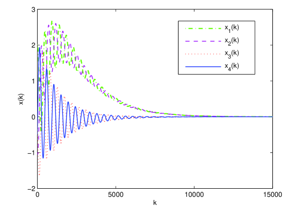
Figure 1: Responses of the satellite system with $h(k)=1+169|\sin(k\pi/2)|$

V Conclusion

In this paper, new summation inequalities in single and double form have been proposed. By employing the newly derived inequalities, improved stability conditions have been derived for a class of discrete-time systems with time-varying delay. Provided examples and comparisons to the most recent results found in the literature show the potential and a large improvement on the stability conditions deliver by the approach proposed in this paper.

References

• [1] R. Sipahi, S.-I. Niculescu, C.T. Abdallah, W. Michiels, and K. Gu. Stability and stabilization of systems with time delay. IEEE Control Systems, 31(1): 38–65, 2011.
• [2] E. Fridman. Introduction to Time-Delay Systems: Analysis and Control, Birkhäuser, 2014.
• [3] E. Fridman, U. Shaked, and K. Liu. New conditions for delay-derivative-dependent stability. Int. J. Control, 45(11): 2723–2727, 2009.
• [4] L.V. Hien, and V.N. Phat. Exponential stability and stabilization of a class of uncertain linear time-delay systems. J. Franklin Inst., 46(6): 611–625, 2009.
• [5] E. Fridman. A refined input delay approach to sampled-data control. Automatica, 46(2): 421–427, 2010.
• [6] A. Seuret. A novel stability analysis of linear systems under asynchronous samplings. Automatica, 48(1): 177–182, 2012.
• [7] A. Seuret, and F. Gouaisbaut. Wirtinger-based integral inequality: Application to time-delay systems. Automatica, 49(9): 2860–2866, 2013.
• [8] L.V. Hien, and H.M. Trinh. A new approach to state bounding for linear time-varying systems with delay and bounded disturbances. Automatica, 50(6): 1735–1738, 2014.
• [9] Y. Li, K. Gu, J. Zhou, and S. Xu. Estimating stable delay intervals with a discretized Lyapunov-Krasovskii functional formulation. Automatica, 50(6): 1691–1697, 2014.
• [10] P.G. Park, W.I. Lee, and S.Y. Lee. Auxiliary function-based integral inequalities for quadratic functions and their applications to time-delay systems. J. Frankl. Inst., 352(4): 1378–1396, 2015.
• [11] P.G. Park, J.W. Ko, and C. Jeong. Reciprocally convex approach to stability of systems with time-varying delays. Automatica, 47(1): 235–238, 2011.
• [12] Z. Feng, J. Lam, and G.H. Yang. Optimal partitioning method for stability analysis of continuous/discrete delay systems. Int. J. Robust Nonlinear Control, 25(4): 559–574, 2015.
• [13] C. Peng. Improved delay-dependent stabilisation criteria for discrete systems with a new finite sum inequality. IET Control Theory Appl., 6(3): 448–453, 2012.
• [14] A. Seuret, and F. Gouaisbaut. Complete quadratic Lyapunov functionals using Bessel-Legendre inequality. European Control Conference (ECC’14), Strasbourg, France, 2014.
• [15] L.V. Hien. A novel approach to exponential stability of nonlinear non-autonomous difference equations with variable delays. Appl. Math. Lett., 38: 7–13, 2014.
• [16] E. Fridman, and U. Shaked. Stability and guaranteed cost control of uncertain discrete delay systems. Int. J. Control, 78(4): 235–246, 2005.
• [17] Y. He, Q. G. Wang, L. Xie, and C. Lin. Further improvement of free-weighting matrices technique for systems with time-varying delay. IEEE Trans. Autom. Control, 52(2): 293–299, 2007.
• [18] B. Zhang, S. Xu, and Y. Zou. Improved stability criterion and its application in delayed controller design for discrete-time systems. Automatica, 44(11): 2963–2967, 2008.
• [19] X.Y. Meng, J. Lam, B.Z. Du, and H.J. Gao. A delay-partitioning approach to the stability analysis of discrete-time systems. Automatica, 46(3): 610–614, 2010.
• [20] H. Shao, and Q.L. Han. New stability criteria for linear discrete-time systems with interval-like time-varying delays. IEEE Trans. Autom. Control, 56(3): 619–625, 2011.
• [21] C.-Y. Kao. On stability of discrete-time LTI systems with varying time delays. IEEE Trans. Automatic Control, 57(5): 1243–1248, 2012.
• [22] O.M. Kwon, M.J. Park, J.H. Park, S.M. Lee and E.J. Cha. Stability and stabilization for discrete-time systems with time-varying delays via augmented Lyapunov-Krasovskii functional. J. Frankl. Inst., 350(3): 521–540, 2013.
• [23] L.V. Hien, N.T. An, and H. Trinh. New results on state bounding for discrete-time systems with interval time-varying delay and bounded disturbance inputs. IET Control Theory Appl., 8(14): 1405–1414, 2014.
• [24] S.H. Kim. Further results on stability analysis of discrete-time systems with time-varying delays via the use of novel convex combination. Appl. Math. Comput., 261: 104–113, 2015.
• [25] P.T. Nam, P.N. Pubudu, and H. Trinh. Discrete Wirtinger-based inequality and its application. J. Frankl. Inst., 352: 1893–1905, 2015.
• [26] A. Seuret, F. Gouaisbaut, and E. Fridman. Stability of discrete-time systems with time-varying delays via a novel summation inequality. IEEE Trans. Autom. Control, doi: 10.1109/TAC.2015.2398885.
• [27] J. Zhang, C. Peng, and M. Zheng. Improved results for linear discrete-time systems with an interval time-varying input delay. Int. J. Syst. Sci., (2014) doi: 10.1080/00207721.2014.891674.
• [28] H. Gao, X.Meng, T. Chen, and J. Lam. Stabilization of networked control systems via dynamic output-feedback controllers. SIAM J. Control Optim., 48(5): 3643–3658, 2010.