A cluster-based mean-field and perturbative description of strongly correlated fermion systems. Application to the 1D and 2D Hubbard model

Abstract

We introduce a mean-field and perturbative approach, based on clusters, to describe the ground state of fermionic strongly-correlated systems. In cluster mean-field, the ground state wavefunction is written as a simple tensor product over optimized cluster states. The optimization of the single-particle basis where the cluster mean-field is expressed is crucial in order to obtain high-quality results. The mean-field nature of the ansatz allows us to formulate a perturbative approach to account for inter-cluster correlations; other traditional many-body strategies can be easily devised in terms of the cluster states. We present benchmark calculations on the half-filled 1D and (square) 2D Hubbard model, as well as the lightly-doped regime in 2D, using cluster mean-field and second-order perturbation theory. Our results indicate that, with sufficiently large clusters or to second-order in perturbation theory, a cluster-based approach can provide an accurate description of the Hubbard model in the considered regimes. Several avenues to improve upon the results presented in this work are discussed.

I Introduction

Despite some substantial recent progress, an accurate and efficient description of the ground and excited states of low-dimensional strongly-correlated fermionic systems represents an open problem in condensed matter physics and quantum chemistry. A common feature in strongly-correlated systems is the collective behavior displayed by fermions in low-lying states. Accordingly, approaches based on composite particles have been proposed for treating these systems. One notorious example is the resonating valence bond as a ground state candidate for high-$T_{c}$ superconductors, as suggested by Anderson Anderson (1987).

In this work, we use composite many-fermion cluster states to describe the ground state of strongly-correlated systems. Here, a cluster is simply a subset of all available single-fermion states that we group (generally using a criterion of proximity in real space). We presume that an accurate zero-th order description of the ground state of the full system can be prepared as a product of cluster states, each being many fermion in character. Two key aspects in obtaining an accurate description are: 1) the many-fermion state in each cluster is determined in the presence of other clusters, and 2) the single-particle basis used to determine the grouping into clusters is fully optimized. This optimization could in principle break the real space localization criterion but in practice it generally does not. The resulting cluster mean-field (cMF) state is, by construction, guaranteed to provide a variational estimate of the ground state energy that is lower than Hartree–Fock (HF), i.e., the standard mean-field of single-particles. The optimization provides not only the optimal cMF state, but also a renormalized Hamiltonian expressed in term of cluster states. Traditional many-body approaches can then be used, on this renormalized Hamiltonian, to account for the missing inter-cluster correlations.

Our work is inspired by McWeeny McWeeny (1959, 1960), who first considered the properties of wavefunctions written as a tensor product of the state of several subsystems (or groups), which are mutually orthogonal. McWeeny realized that the density matrix of cluster product states can be easily expressed in terms of the density matrices of the individual clusters. In related work, Isaev, Ortiz, and Dukelsky Isaev et al. (2009) considered, in their hierarchical mean-field (HMF) approach, a similar ansatz to ours for the 2D Heisenberg Hamiltonian. We note, nevertheless, that the generalization to fermionic systems of the HMF approach used in Ref. Isaev et al., 2009 is not straightforward if the full Fock space within each cluster is treated. An attempt was performed in Ref. Zhao et al., 2014 to split the Fock space in each cluster according to its number parity: states with even (odd) parity where treated as bosonic (fermionic) degrees of freedom. An ansatz for the ground state was constructed in Ref. Zhao et al., 2014 as a tensor product of the bosonic and fermionic degrees of freedom; this decoupling, however, may not be justified in all cases and can potentially result in unphysical states.

Our approach differs from that used in Ref. Isaev et al., 2009, aside from the application to fermionic systems, in not requiring the individual clusters to share the same ground state. That is, the ground state of each cluster is optimized independently allowing for (translational and spin) symmetry-broken solutions. In addition, we here consider Rayleigh-Schrödinger perturbation theory (RS-PT) Schrödinger (1926) to second-order as a means to obtain a correlated approach defined in terms of clusters.

A closely related cluster product approach was also proposed by Li Li (2004). In that work, the ground state of each cluster was, nonetheless, not optimized in the presence of other clusters. The author did, on the other hand, go beyond perturbation theory into a coupled-cluster ansatz (so-called block-correlated coupled cluster (BCCC)) as a way to correlate the cluster product state. The BCCC approach has been used with high success in quantum chemistry to describe strongly-correlated molecular systems using either a complete active-space Fang et al. (2008); Shen and Li (2009) or generalized valence-bond Xu and Li (2013) reference states.

A cluster product state is naturally connected with the tensor network (TN) techniques that have been gaining popularity for treating strongly-correlated systems Cirac and Verstraete (2009); Orús (2014). In essence, the cluster product state is the simplest possible TN, a simple scalar (the bond or ancillary index dimension is set to 1), although the elements defining the network are chosen as cluster states rather than single-particle degrees of freedom as often done. The consequence of using a scalar product is that the clusters become disentangled; more general TNs such as the matrix product states (MPS) used within the density matrix renormalization group algorithm (DMRG) White (1992, 1993) introduce entanglement in the ansatz and can provide highly accurate solutions for strongly-correlated systems. The optimization of TN states beyond the simple MPS is, however, non-trivial and remains an area of active research Orús (2014).

Yet other wavefunction ansätze that are related to the cluster product states are the correlator product states (CPS) Changlani et al. (2009) or entangled plaquette states (EPS) Mezzacapo et al. (2009); Mezzacapo and Cirac (2010). Here, a variational ansatz is expressed in terms of entangled cluster products, as opposed to a simple uncorrelated product. The price to pay is that the evaluation of matrix elements becomes more cumbersome, and it often has to be carried out by stochastic means (within a variational Monte Carlo framework). We note that Ref. Neuscamman et al., 2011 proposed a non-stochastic algorithm for optimizing CPS.

At this point, we want to clarify why we have decided to use simple cluster product states even when more powerful ansätze are already available (such as more general TNs or CPS). In our perspective, the power of a cluster mean-field approach has not been fully realized. In particular, symmetry breaking and orbital optimization can partially account for inter-cluster correlations (when expressed in terms of the original set of fermion states). Moreover, the fact that the cluster mean-field state constitutes the ground state of a mean-field Hamiltonian of which the full set of eigenstates can be easily constructed has often been overlooked. This allows us to formulate a perturbative strategy to introduce the missing inter-cluster correlations. Yet more powerful many-body approaches (such as coupled-cluster theory) can be easily introduced as done by Li in the BCCC method.

Our objective with this work is thus two-fold. First, we present the cMF formalism as well as provide details of the RS-PT formulation we use. (We refer to the second-order perturbative result as cPT2 in the remainder of this paper.) We describe in some detail the strategy used to optimizate the one-electron basis in which the cMF state is expressed. Our second objective is to apply these techniques to the simplest paradigm of strongly-correlated fermionic systems: the Hubbard model Hubbard (1963) in one- (1D) and two-dimensions (2D) in a square lattice. The 1D case is exactly solvable Lieb and Wu (1968), while the 2D model has been extensively studied. We refer the reader to Refs. Scalapino, 2007; LeBlanc et al., 2015 for a survey of numerical methods applied to the 2D Hubbard model. We compare our results with second-order unrestricted Møller-Plesset (UMP2) Møller and Plesset (1934) and unrestricted coupled-cluster with singles and doubles (UCCSD) Shavitt and Bartlett (2009), as well as with perturbative triples (UCCSD(T)), calculations. MP2 constitutes second-order RS-PT based on a HF wavefunction (using canonical orbital and orbital energies), while coupled-cluster constitutes a non-perturbative approach that involves an infinite-order resummation of diagrams. Our results show that cMF (cPT2) significantly improves upon HF (MP2) and can provide an accurate description of the ground state of the Hubbard model.

The remainder of this work is organized as follows. In Sec. II we present the formalism behind cMF and cPT2. Section III provides some practical computational details regarding the calculations presented in this work. In Sec. IV we present the results of cMF and cPT2 calculations for the half-filled 1D and 2D Hubbard model, as well as for the lightly-doped 2D regime. A brief discussion following the results is presented in Sec. V, along with some ideas as to how to improve the calculations here presented. Lastly, Sec. VI is devoted to some general conclusions. In Appendix A we show higher order perturbation results in a small lattice, while in Appendix B we discuss the applicability of cMF to weakly correlated systems.

II Formalism

II.1 Hubbard model

In this work, we focus our attention on the Hubbard model in one- and two-dimensions (in a square lattice). The Hubbard model Hubbard (1963) describes a collection of electrons in a lattice (of finite size $L$) interacting through the Hamiltonian

$$\hat{H}=-t\sum_{\langle ij\rangle,\sigma}(c^{\dagger}_{i,\sigma}\,c_{j,\sigma}+\textrm{h.c.})+U\sum_{i}n_{i,\uparrow}\,n_{i,\downarrow},$$ (1)

where the notation $\langle ij\rangle$ implies interaction only among nearest-neighbors. Here, $c^{\dagger}_{i,\sigma}$ ($c_{i,\sigma}$) creates (annihilates) an electron with spin $\sigma$ on site $i$ of the lattice and $n_{i,\sigma}\equiv c^{\dagger}_{i,\sigma}\,c_{i,\sigma}$. The Hamiltonian contains one-electron hopping terms and an on-site repulsion ($U>0$) term. The hopping amplitude $t$ is used to set the energy scale.

II.2 Cluster Mean-Field

Consider a set of single-fermion states $\{|k\rangle,\,k=1,\ldots,M\}$, where $M$ is the size of the basis, that satisfies the appropriate set of boundary conditions for the system. These single-fermion states may be different than the ones used to define the problem; in the case of the Hubbard model, they may be obtained by a rotation of the lattice (on-site) basis states:

$$|k\rangle\equiv \,a^{\dagger}_{k}|-\rangle,$$ (2)

$$a^{\dagger}_{k}= \,\hat{R}\,c^{\dagger}_{k}\,\hat{R}^{-1}.$$ (3)

We assume that $a^{\dagger}_{k}$ and $a_{k}$ satisfy standard anti-commutation rules (implying orthonormality of $\{|k\rangle\}$). A basis for many-fermion states can be constructed from properly antisymmetrized products of such single-fermion states.

Let the single-fermion states be grouped, according to some criterion (such as proximity in real space), into clusters of size $l_{1},l_{2},\ldots l_{n}$, where $n$ is the number of such clusters. The Fock space in each cluster can be constructed using the single-fermion states that define it. Due to the orthogonality of single-fermion states in different clusters, the Fock space of the full system is simply given by the tensor product of the Fock spaces of all clusters.

A second-quantized formulation in terms of cluster product states can also be established. Let $A^{\dagger}_{I,c}$ ($A_{I,c}$) create (annihilate) the $I$-th many-fermion state in cluster $c$. This $I$-th state is a linear combination of many-fermion basis states $\{|\mu\rangle_{c}\}$ (possibly mixing states with different number of fermions) constructed as antisymmetrized products of the single-fermion states in the cluster. We formally write

$$|I\rangle_{c}=A^{\dagger}_{I,c}|-\rangle_{c},$$ (4)

where $|-\rangle_{c}$ is the vacuum state in cluster $c$. (We emphasize here that $|-\rangle_{c}$ does not correspond to the state with no fermions in the cluster, but is simply a useful abstract construct.)

An arbitrary state $|\Psi\rangle$ in the Fock space of the entire system can be formed as

$$|\Psi\rangle=\sum_{I}\sum_{J}\cdots\sum_{Z}c_{I1;J2;\ldots;Zn}\,|I\rangle_{1}|J\rangle_{2}\cdots|Z\rangle_{n},$$ (5)

where $c_{I1;J2;\ldots;Zn}$ are linear coefficients. Here, the sum over $I$ spans the full Fock space in cluster 1, and so on. Each state in the expansion above constitutes a cluster product state. Formally, each cluster product state is built as

$$|I\rangle_{1}|J\rangle_{2}\cdots|Z\rangle_{n}\equiv A^{\dagger}_{I,1}\,A^{\dagger}_{J,2}\cdots A^{\dagger}_{Z,n}|-\rangle,$$ (6)

where $|-\rangle$ is an abstract vacuum state for the full system.

In this work, we consider a cluster product (mean-field) state as a variational ansatz for the ground state wavefunction. That is, the ansatz $|\Phi_{0}\rangle$ for the ground state is given by

$$|\Phi_{0}\rangle=|0\rangle_{1}|0\rangle_{2}\cdots|0\rangle_{n},$$ (7)

where we have indicated that the ground state (hence the $0$ label) in each cluster is used to build the product state. The optimal cMF state is obtained by a variational minimization scheme, as outlined in Sec. II.4.

Having defined a ground state cluster product configuration, excited configurations can also be considered. We write them as

$$|\Phi_{Ii}\rangle= \,|0\rangle_{1}\cdots|I\rangle_{i}\cdots|0\rangle_{n},$$ (8)

$$|\Phi_{Ii;Jj}\rangle= \,|0\rangle_{1}\cdots|I\rangle_{i}\cdots|J\rangle_{j}\cdots|0\rangle_{n},$$ (9)

$$|\Phi_{Ii;Jj;Kk}\rangle= \,|0\rangle_{1}\cdots|I\rangle_{i}\cdots|J\rangle_{j}\cdots|K\rangle_{k}\cdots|0\rangle_{n},$$ (10)

for singly-, doubly-, and triply-excited clusters. A full configuration expansion can be written in terms of excited configurations as

$$|\Psi\rangle= \,c_{0}|\Phi_{0}\rangle+\sum_{i}\sum_{I\neq 0}c_{Ii}|\Phi_{Ii}\rangle$$

$$\,+\sum_{i<j}\sum_{I\neq 0}\sum_{J\neq 0}c_{Ii;Jj}|\Phi_{Ii;Jj}\rangle+\ldots$$ (11)

This provides exact eigenstates for the full system.

Before proceeding further, let us comment on the nature of the cluster product states considered in this work. We indicated above that the ground state of each cluster is expressed as a linear combination of the many-fermion basis states in it. That is,

$$|0\rangle_{c}=\sum_{\mu}d_{0,c}^{\mu}|\mu\rangle_{c},$$ (12)

with $d_{0,c}^{\mu}={}_{c}\langle\mu|0\rangle_{c}$, where $\mu$ is a compound index of occupation numbers in the subset of single-fermion states of the cluster. The expansion over states $\{|\mu\rangle_{c}\}$ can be restricted, i.e., some of the $\{d_{0,c}^{\mu}\}$ coefficients may be set to 0. We note that if a given cluster state is expanded in terms of even- and odd-number parity (here referring to an even or odd number of fermions) states, commutation rules between the operators $A^{\dagger}_{I,c}$ and $A_{J,c^{\prime}}$ are not simple, complicating the evaluation of matrix elements as hinted below. All the calculations included in this work restrict the expansion of cluster states to a given $n_{\uparrow}$ and $n_{\downarrow}$ (or, equivalently, $n$ and $m_{s}$) sector within the cluster, but include the full Hilbert subspace with those quantum numbers. This was done in order for the cluster product state $|\Phi_{0}\rangle$ to be an eigenfunction of $\hat{N}_{\uparrow}$ and $\hat{N}_{\downarrow}$.

Consider the determinantal expansion of the full system. The exact ground state wavefunction is expressed as

$$|\Psi\rangle=\sum_{\mu\nu\lambda\cdots}c_{\mu\nu\lambda\cdots}|\mu\nu\lambda\cdots\rangle,$$ (13)

including all possible many-fermion states $\{|\mu\rangle_{c}\}$ within the cluster. In cMF, the coefficients in the expansion above are not independent, but are parametrized according to

$$c_{\mu\nu\lambda\cdots}=d_{0,1}^{\mu}\,d_{0,2}^{\nu}\,d_{0,3}^{\lambda}\cdots.$$ (14)

This parametrization permits us to put cMF in the context of TN states Cirac and Verstraete (2009); Orús (2014) and CPS Changlani et al. (2009); Mezzacapo et al. (2009); Mezzacapo and Cirac (2010). In cMF the coefficient of each determinant is parametrized as a scalar product of cluster states (with compound indices). That is, the cluster product state has intra-cluster correlations, but lacks inter-cluster ones. This is in contrast to a TN state, where ancillary or bond indices include explicit entanglement in the ansatz. While in cMF the compound indices $\mu$, $\nu$, etc. refer to different orbital subspaces, CPS use overlapping indices as a means of introducing entanglement in the ansatz. The optimization of TN states and CPS is, nonetheless, more involved than that of cMF states.

A cMF state constitutes a generalization of a single Slater determinant, and thus HF can be written as a cMF where the orbitals are grouped into clusters, as we next describe. It should be stressed that this is only possible in the optimized single-particle basis (or a unitary rotation of it that does not mix particles with holes). The HF state is recovered in different ways: as a product of two clusters (one fully occupied and one fully empty), or as a product of $M$ clusters (the holes being occupied and the particles being empty), or arbitrary related constructions.

The model also contains other wavefunction ansätze commonly used in quantum chemistry such as the antisymmetrized product of strongly orthogonal geminals (APSG) Parks and Parr (1958); Surján (1999); Rassolov (2002). Here, each cluster would contain two-electrons in a subspace of orbitals that define each geminal. It also encompasses the multi-configuration self-consistent-field (MC-SCF) Hartree et al. (1939); Shepard (2007) model as well as the complete-active-space (CAS) Roos et al. (1980); Roos (2007) variant of it. The latter can be considered as a three-cluster state: the core is fully occupied, the virtual set of orbitals is fully empty, and the state in the active space is expressed as an optimized linear combination of all possible many-electron basis states in the appropriate Hilbert space.

II.3 Matrix Elements

We now turn to the evaluation of matrix elements over cMF states. The (two-body) fermionic Hamiltonian is expressed in second-quantized form (in the basis that defines the clusters) as

$$\hat{H}=\sum_{pr}\langle p|\hat{t}|r\rangle a^{\dagger}_{p}\,a_{r}+\frac{1}{2}\sum_{pqrs}\langle pq|\hat{v}|rs\rangle a^{\dagger}_{p}\,a^{\dagger}_{q}\,a_{s}\,a_{r},$$ (15)

where $\langle p|\hat{t}|r\rangle$ are one-body and $\langle pq|\hat{v}|rs\rangle$ are two-body integrals. The Hamiltonian can be expressed as a sum of single, two, three, and four-cluster interactions:

$$\hat{H}=\sum_{i}\hat{H}_{i}+\sum_{i<j}\hat{H}_{ij}+\sum_{i<j<k}\hat{H}_{ijk}+\sum_{i<j<k<l}\hat{H}_{ijkl}.$$ (16)

Here, for instance,

$$\hat{H}_{ij}= \,\sum_{p\in i,r\in j}\Big{(}\langle p|\hat{t}|r\rangle a^{\dagger}_{p}\,a_{r}+\langle r|\hat{t}|p\rangle a^{\dagger}_{r}\,a_{p}\Big{)}$$

$$\,+\frac{1}{2}\sum_{pr\in i,qs\in j}\langle pq|\hat{v}|rs\rangle\,a^{\dagger}_{p}\,a^{\dagger}_{q}\,a_{s}\,a_{r}+\ldots,$$ (17)

$$\hat{H}_{ijkl}= \,\frac{1}{2}\sum_{\begin{subarray}{c}p\in i,q\in j,\\ r\in k,s\in l\end{subarray}}\langle pq|\hat{v}|rs\rangle\,a^{\dagger}_{p}\,a^{\dagger}_{q}\,a_{s}\,a_{r}+\ldots.$$ (18)

Given that fermion operators $\{a^{\dagger}_{p},a_{p}\}$ act on specific clusters, the matrix elements can be evaluated straightforwardly if all the cluster states have a well defined number parity (though care has to be taken to respect fermionic anti-commutation rules). For instance,

$$\mathrm{if}\,p\in 2\qquad a^{\dagger}_{p}|\Phi_{0}\rangle=\pm|0\rangle_{1}\,a^{\dagger}_{p}|0\rangle_{2}|0\rangle_{3}\cdots,$$ (19)

where the sign depends on the number parity of $|0\rangle_{1}$. (The action of $a^{\dagger}_{p}$ ($a_{p}$) on a specific cluster can be easily expressed in the occupation number basis $\{|\mu\rangle_{c}\}$ within each cluster.) If $|0\rangle_{c}$ is of mixed number parity, the evaluation becomes more cumbersome. For instance,

$$\mathrm{if}\,p\in 2\qquad a^{\dagger}_{p}|\Phi_{0}\rangle= +\,|0\rangle_{1}^{+}\,a^{\dagger}_{p}|0\rangle_{2}|0\rangle_{3}\cdots$$

$$-\,|0\rangle_{1}^{-}\,a^{\dagger}_{p}|0\rangle_{2}|0\rangle_{3}\cdots,$$ (20)

where $|0\rangle_{1}^{+}$ denotes the even-number parity projection out of $|0\rangle_{1}$, i.e., $|0\rangle_{1}^{+}\equiv|+\rangle\langle+|0\rangle_{1}$.

We close this section by noting that, if the ground state in each cluster preserves number parity, then expectation values of single-fermion operators (such as ${}_{c}\langle 0|a_{p}^{\dagger}|0\rangle_{c}$, for $p\in c$) vanish. This further implies that all three- and four-cluster interactions vanish in $\langle\Phi_{0}|\hat{H}|\Phi_{0}\rangle$. If the number of fermion states within each cluster is fixed, then the expectation value $\langle\Phi_{0}|\hat{H}|\Phi_{0}\rangle$ can be fully expressed in terms of the one- and two-particle reduced density matrices within each cluster, as first noted by McWeeny McWeeny (1959). (Note that this implies that the cost of evaluating the energy of a cMF state scales as $\mathcal{O}(n^{2})$, where $n$ is the number of clusters used.)

II.4 cMF Optimization

In this section we discuss how the cMF state is optimized, that is, how the ground state $|0\rangle_{c}$ in each cluster $c$ is determined. We use a diagonalization strategy akin to that used in HF or multi-configuration self-consistent-field (MC-SCF) methods.

The optimal set of coefficients $\{d_{0,c}^{\mu}\}$ (cf. Eq. 12) can be found by minimization of the energy subject to the constraint that the state $|0\rangle_{c}$ remains normalized:

$$\frac{\partial}{\partial d_{0,c}^{\mu\ast}}\langle\Phi_{0}|\hat{H}|\Phi_{0}\rangle-\epsilon_{0,c}d_{0,c}^{\mu}=0.$$ (21)

where $\epsilon_{0,c}$ is introduced as a Lagrange multiplier. The above equation can be cast as an eigenvalue equation that, at the same time, defines a zero-th order Hamiltonian $\hat{H}^{0}_{c}$ within the cluster, i.e.,

$$\hat{H}^{0}_{c}\,d_{0,c}^{\mu}\equiv\frac{\partial}{\partial d_{0,c}^{\mu\ast}}\langle\Phi_{0}|\hat{H}|\Phi_{0}\rangle.$$ (22)

The ground state of the cluster Hamiltonian is obtained as its lowest energy eigenvector. (Note that this also gives $\epsilon_{0,c}$ the physical meaning of the energy in cluster $c$.) The cluster Hamiltonian can be found trivially. As an example, if all cluster ground states $\{|0\rangle_{c}\}$ have a fixed number of fermions, $\hat{H}^{0}_{c}$ is given by

$$\hat{H}^{0}_{c}= \,\sum_{pr\in c}\langle p|\hat{t}|r\rangle a^{\dagger}_{p}\,a_{r}+\frac{1}{2}\sum_{pqrs\in c}\langle pq|\hat{v}|rs\rangle a^{\dagger}_{p}\,a^{\dagger}_{q}\,a_{s}\,a_{r}$$

$$+ \,\sum_{pr\in c}a^{\dagger}_{p}\,a_{r}\sum_{c^{\prime}}\sum_{qs}\rho^{c^{\prime}}_{sq}(\langle pq|\hat{v}|rs\rangle\,-\langle pq|\hat{v}|sr\rangle).$$ (23)

Here, $\rho^{c^{\prime}}_{sq}={}_{c^{\prime}}\langle 0|a^{\dagger}_{q}\,a_{s}|0\rangle_{c^{\prime}}$ is the one-particle density matrix in cluster $c^{\prime}$. Because the cluster Hamiltonian $\hat{H}^{0}_{c}$ depends on the ground state density matrices of other clusters, the equations must be solved self-consistently. This represents a generalization of the MC-SCF method, where there are several active subspaces (the clusters) each with its own multi-configurational expansion.

II.5 Orbital Optimization

As discussed in the introduction, in order to realize the full capability of cMF states it is necessary to include the optimization of the single-fermion basis in which the grouping into clusters is defined, which we refer to as an orbital optimization. Otherwise, a cMF state may yield an energy that is even above HF, despite having significantly more flexibility in the ansatz. We describe in this section how this is accomplished in our work. We note that the orbital optimization in cMF states is akin to the same process performed in traditional MC-SCF (and CAS, by extension) calculations in quantum chemistry.

Given the single-particle basis $\{|k\rangle\}$ in which the cMF state is constructed, we aim to rotate this to a new basis $\{|\bar{k}\rangle\}$ in order to lower the energy. We relate the two basis by a unitary transformation (parametrized as the exponential of an anti-Hermitian operator),

$$\bar{a}^{\dagger}_{k}= \,\exp(\hat{\kappa})\,a_{k}\,\exp(-\hat{\kappa}),$$ (24)

$$\hat{\kappa}= \,\sum_{p<q}(\kappa_{pq}\,a^{\dagger}_{p}\,a_{q}-\mathrm{h.c.}).$$ (25)

In particular, we define an energy functional

$$E[\boldsymbol{\kappa}]=\langle\Phi_{0}|\exp(-\hat{\kappa})\,\hat{H}\,\exp(\hat{\kappa})|\Phi_{0}\rangle,$$ (26)

where the (complex) elements $\{\kappa_{pq}\}$ serve as variational parameters.

With the optimized cMF state $|\Phi_{0}\rangle$ at hand, we can compute the gradient with respect to orbital rotations at $\boldsymbol{\kappa}=\mathbf{0}$ (i.e., the gradient evaluated at zero-rotation) as

$$G_{pq}\equiv\left.\frac{\partial E}{\partial\kappa_{pq}^{\ast}}\right|_{\boldsymbol{\kappa}=\boldsymbol{0}}=-\Big{\langle}\Phi_{0}\Big{|}\big{[}\hat{H},a_{q}^{\dagger}\,a_{p}\big{]}\Big{|}\Phi_{0}\Big{\rangle}.$$ (27)

Similarly, the Hessian can be constructed as

$$\mathbf{H}=\begin{pmatrix}\mathbf{A}&\mathbf{B}\\ \mathbf{B}^{\ast}&\mathbf{A}^{\ast}\end{pmatrix},$$ (28)

with

$$A_{pq,rs}\equiv \,\left.\frac{\partial^{2}E}{\partial\kappa_{ij}^{\ast}\,\partial\kappa_{kl}}\right|_{\boldsymbol{\kappa}=\boldsymbol{0}}$$

$$= \,-\frac{1}{2}\Big{\langle}\Phi_{0}\Big{|}\big{[}\big{[}\hat{H},a_{q}^{\dagger}\,a_{p}\big{]},a_{r}^{\dagger}\,a_{s}\big{]}\Big{|}\Phi_{0}\Big{\rangle}$$

$$\,+q,p\leftrightarrow r,s,$$ (29)

$$B_{pq,rs}\equiv \,\left.\frac{\partial^{2}E}{\partial\kappa_{pq}^{\ast}\,\partial\kappa_{rs}^{\ast}}\right|_{\boldsymbol{\kappa}=\boldsymbol{0}}$$

$$= \,+\frac{1}{2}\Big{\langle}\Phi_{0}\Big{|}\big{[}\big{[}\hat{H},a_{q}^{\dagger}\,a_{p}\big{]},a_{s}^{\dagger}\,a_{r}\big{]}\Big{|}\Phi_{0}\Big{\rangle}$$

$$\,+q,p\leftrightarrow s,r.$$ (30)

The gradient (and Hessian) can be used to find a direction of energy lowering with respect to orbital rotations. Several comments are in order:

• The energy and Hessian can be evaluated following the strategy described in Sec. II.3 for the evaluation of matrix elements. It can be shown that the cost of building the full gradient and Hessian scales as $\mathcal{O}(n^{3})$ and $\mathcal{O}(n^{4})$, respectively, where $n$ is the number of clusters in the system.

• Once a direction of energy lowering is found (defining a non-zero $\boldsymbol{\kappa}$), we perform a finite rotation ($\alpha\boldsymbol{\kappa}$) of the Hamiltonian integrals. The energy functional is re-parametrized with respect to orbital rotations in terms of the new single-particle basis.

• The above strategy (re-parametrizing the energy functional at each step) is necessary as the evaluation of the orbital gradient (and Hessian) is not as simple when $\boldsymbol{\kappa}\neq\mathbf{0}$. This also prevents us from using a quasi-Newton strategy to perform the orbital optimization.

• Care has to be taken of handling linear dependencies between the orbital rotations and the coefficients in each cluster expansion. For instance, if a cluster state $|0\rangle_{c}$ is expanded in terms of a full Hilbert (or Fock) subspace, then orbital rotations within the subset of orbitals that define the cluster $c$ do not lower the energy.

In this work, as we use a full Hilbert subspace to describe each cluster, the orbital gradient and Hessian for intra-cluster rotations are not considered as degrees of freedom.

II.6 Perturbation Theory

In standard RS-PT Schrödinger (1926), we aim to solve for the eigenstates of the Hamiltonian $\hat{H}$ given the simpler Hamiltonian $\hat{H}^{0}$, for which all eigenstates are known. In RS-PT, the second-order correction to the ground state energy is evaluated as

$$E^{(2)}=\sum_{\mu\neq 0}\frac{|V_{0\mu}|^{2}}{\varepsilon_{0}-\varepsilon_{\mu}},$$ (31)

where $\hat{V}=\hat{H}-\hat{H}^{0}$ and $V_{0\mu}=\langle\Phi_{0}|\hat{V}|\mu\rangle$. Here, $\mu$ labels the eigenstates of $\hat{H}_{0}$ and $\varepsilon_{\mu}$ are the corresponding eigenvalues.

The cMF state, as outlined in Sec. II.4, provides a natural zero-th order Hamiltonian of which all eigenstates can be easily constructed. This is expressed as a direct sum of the zero-th order Hamiltonians of each cluster

$$\hat{H}^{0}=\hat{H}^{0}_{1}+\hat{H}^{0}_{2}+\ldots$$ (32)

The eigenstates of such Hamiltonian are given by

$$\hat{H}^{0}|I\rangle_{1}|J\rangle_{2}\cdots|Z\rangle_{n},= \,\varepsilon_{I1;J2;\cdots;Zn}|I\rangle_{1}|J\rangle_{2}\cdots|Z\rangle_{n}$$ (33)

$$\varepsilon_{I1;J2;\cdots;Zn}= \,\epsilon_{1,I}+\epsilon_{2,J}+\cdots+\epsilon_{n,Z}.$$ (34)

As described in Sec. II.3, $\hat{H}$ has up to four-cluster interactions, while $\hat{H}^{0}$ is, by construction, single-cluster in character. If a full Hilbert subspace in each cluster is used, matrix elements between the ground state $|\Phi_{0}\rangle$ and singly-excited (cluster) configurations vanish due to a generalized-Brillouin condition. Therefore, only two, three, and four-cluster interactions contribute to the second-order energy. The evaluation of the corresponding matrix elements can be carried out in a similar fashion as the evaluation of $\langle\Phi_{0}|\hat{H}|\Phi_{0}\rangle$. Naturally, computing the four-cluster interactions is the most expensive step in evaluating the second-order energy, with a computational scaling of $\mathcal{O}(n^{4})$ in the number of clusters.

As described in Sec. II.2, in this work we have chosen to use cluster ground states which preserve the number of $\uparrow$- and $\downarrow$-electrons. In that case, several two, three, and four-cluster interaction channels can be identified in the Hamiltonian, as summarized in Tab. 1. The cMF ground state $|\Phi_{0}\rangle$ interacts with excited cluster configurations following these channels.

Table 1: Two-, three-, and four-cluster interaction channels when the ground state in each cluster has well defined $n_{\uparrow}$ and $n_{\downarrow}$.

# clusters	type	sample interaction	restrictions
2	one-electron CT	$a^{\dagger}_{p,\sigma}\,a^{\dagger}_{q,\sigma^{\prime}}\,a_{s,\sigma^{\prime}}\,a_{r,\sigma}$	$pqs\in i$, $r\in j$
2	two-electron, opp spin, CT	$a^{\dagger}_{p,\sigma}\,a^{\dagger}_{q,-\sigma}\,a_{s,-\sigma}\,a_{r,\sigma}$	$pq\in i$, $sr\in j$
2	two-electron, same spin, CT	$a^{\dagger}_{p,\sigma}\,a^{\dagger}_{q,\sigma}\,a_{s,\sigma}\,a_{r,\sigma}$	$pq\in i$, $sr\in j$
2	two-cluster spin flip	$a^{\dagger}_{p,\sigma}\,a^{\dagger}_{q,-\sigma}\,a_{s,-\sigma}\,a_{r,\sigma}$	$ps\in i$, $qr\in j$
2	two-cluster dispersion	$a^{\dagger}_{p,\sigma}\,a^{\dagger}_{q,\sigma^{\prime}}\,a_{s,\sigma^{\prime}}\,a_{r,\sigma}$	$pr\in i$, $qs\in j$
3	two-electron, opp spin, CT	$a^{\dagger}_{p,\sigma}\,a^{\dagger}_{q,-\sigma}\,a_{s,-\sigma}\,a_{r,\sigma}$	$pq\in i$, $s\in j$, $r\in k$
3	two-electron, same spin, CT	$a^{\dagger}_{p,\sigma}\,a^{\dagger}_{q,\sigma}\,a_{s,\sigma}\,a_{r,\sigma}$	$pq\in i$, $s\in j$, $r\in k$
3	single-cluster spin flip	$a^{\dagger}_{p,\sigma}\,a^{\dagger}_{q,-\sigma}\,a_{s,-\sigma}\,a_{r,\sigma}$	$ps\in i$, $q\in j$, $r\in k$
3	one-electron CT + dispersion	$a^{\dagger}_{p,\sigma}\,a^{\dagger}_{q,\sigma^{\prime}}\,a_{s,\sigma^{\prime}}\,a_{r,\sigma}$	$pr\in i$, $q\in j$, $s\in k$
4	two-electron scattering	$a^{\dagger}_{p,\sigma}\,a^{\dagger}_{q,\sigma^{\prime}}\,a_{s,\sigma^{\prime}}\,a_{r,\sigma}$	$p\in i$, $q\in j$, $s\in k$, $r\in l$

At this point, we clarify that in this work the zero-th order cluster Hamiltonian is used, without any modification, to generate the full Fock space within the cluster. It is possible to tweak the definition of the non-interacting Hamiltonian (e.g., by adding a level-shift) in specific Hilbert space subsectors in order to improve the convergence properties of the perturbation series.

III Computational Details

The cMF and cPT2 calculations presented in this work were carried out with a locally prepared code. Most of the results use an unrestricted cMF (U-cMF) formalism, where $\uparrow$-orbitals are allowed to have a different spatial distribution than $\downarrow$-ones. Some of the results in 1D lattices use a restricted (R-cMF) formalism, where the spatial distribution is required to be the same. Real orbitals are used in both cases. In all the calculations we use the same number of $\uparrow$- and $\downarrow$-orbitals in each cluster, which we denote as $l$ and refer to as the size of the cluster. The number of $\uparrow$- and $\downarrow$-electrons in each cluster was held fixed (thus preserving $n$ and $m_{s}$ within each cluster). Although not enforced from the outset, R-cMF calculations resulted in spin singlet eigenstates within each cluster.

The full relevant $m_{s}$ sector of Hilbert space within each cluster was used in constructing the cluster ground state $|0\rangle_{c}$. For small cluster sizes, the ground state in each cluster was found by a standard diagonalization of the local cluster Hamiltonian. For larger cluster sizes, a Lanczos Lehoucq et al. (1998) or a Jacobi-Davidson Davidson (1975); Sleijpen and Van der Vorst (1996) algorithm was used to solve for the ground state.

The orbital optimization was carried out using a pseudo Newton-Raphson approach. After optimizing the cluster mean-field state, a Newton step was taken in the direction of energy lowering (using the orbital gradient and Hessian). A finite rotation provided a new single-particle basis in which the cluster mean-field was reoptimized. These two steps were alternated until convergence was achieved in both the cMF state and the orbitals. This is akin to the most common methods of optimizing MC-SCF wavefunctions in quantum chemistry Yeager and Jørgensen (1979); Douady et al. (1980); Siegbahn et al. (1981). We note that a full Newton-Raphson approach (with the mean-field and the orbital optimization carried out concomitantly) should be preferred Werner and Meyer (1980), but we have not used it in this work. A globally convergent algorithm was used to guarantee that the variational cMF energy is reduced in each orbital optimization step. As described in detail below, for 2D lattices several local minima can be found in the orbital optimization process. We have not attempted to use an algorithm to locate the global minimum.

In U-cPT2 calculations, all relevant cluster states were used in computing the second-order energy for small cluster sizes ($l=2$ and $l=3$). For $l=4$ and $l=5$, the four-cluster contributions were computed using only 16 states in each Hilbert subspace of a cluster, while two- and three-tile contributions used all available states. In $l=6$ calculations we truncated the number of states in each Hilbert subspace in three- (four)-tile interactions to 64 (16), while no truncation was done in computing two-tile interactions. An energy-based criterion for the cluster states was used to carry out the truncation. We should point out that the second-order energy appears to be converged in all cases with respect to the number of states included.

UCCSD and UCCSD(T) calculations were carried out with a locally modified version of the MRCC code Kállay and Surján (2001); Kállay et al. . Exact solutions to the 1D Hubbard lattice were obtained by solving the Lieb-Wu Lieb and Wu (1968) equations.

IV Results

In this section we present results of cMF and cPT2 calculations on the 1D and 2D Hubbard models. We start by providing an illustrative example in Sec. IV.1, where we get into some practical details regarding the optimization of cMF states and the way in which other results are presented. In Sec. IV.2 we consider the 1D half-filled case, for which exact solutions are available. We then proceed to study the 2D half-filled case in Sec. IV.3, and finally consider the lightly-doped 2D case in Sec. IV.4. Our 2D results are compared to highly accurate numerical estimates from Refs. LeBlanc et al., 2015; Zheng and Chan, 2015.

IV.1 Illustrative example

In this section we discuss some practical aspects regarding the optimization of cMF states. In this way, we hope that the results presented in subsequent sections will become more transparent to the reader. We consider a 12-site Hubbard 1D periodic lattice at half-filling and $U/t=4$. For U-cMF calculations, we typically start from an unrestricted HF (UHF) solution; we take the resulting orbitals and perform a Boys localization Kleier et al. (1974). Figure 1 displays, in the top-left scheme, (localized) occupied and virtual spin-orbitals mostly tied to two sites, which are then used to define a cluster of 2-$\uparrow$ and 2-$\downarrow$ orbitals in which a single electron of each spin is placed. The optimized state in the cluster is expressed as a linear combination of the 4 possible resulting configurations.

After setting the initial orbitals and the corresponding tiling scheme (i.e., defining how orbitals and electrons are grouped into clusters), the cluster mean-field state is optimized by a self-consistent diagonalization of the appropriate cluster Hamiltonians. The orbital gradient (and possibly the Hessian) is then evaluated which determines how orbitals in different clusters should be mixed in order to lower the energy. A new orbital basis is defined by, e.g., a steepest-descent step, and the cluster mean-field step is reoptimized in such basis. The process is repeated until convergence is reached in both the orbitals and the mean-field state. The top-right scheme in Fig. 1 shows the converged orbitals that define a single cluster in the calculation. In particular, the orbitals displayed are the natural orbitals (those that diagonalize the $\uparrow$- and $\downarrow$- one-particle reduced density matrix) mostly tied to the original two sites. The orbitals defining the cluster remain well localized in two lattice sites (although there is a noticeable spread into neighboring sites which becomes more pronounced at lower $U/t$). This allows us to, for simplicity purposes, characterize the optimized solution in terms of a tiling scheme in the on-site basis (see bottom of the figure), although we emphasize that this is only approximate. In this case, the structure is defined by local dimers which are spin polarized (with a non-zero magnetization in each site) to yield an overall Néel-like configuration.

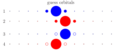
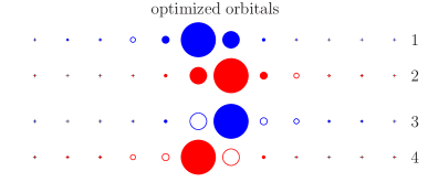
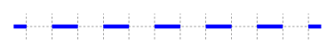
Figure 1: (Color online) In the top schemes we show initial guess (left) and optimized (right) spin-orbitals that define a single cluster in an U-cMF calculation (12-site half-filled periodic 1D lattice, $U/t=4$) using clusters of 2 $\uparrow$- and 2 $\downarrow$-orbitals with 1 $\uparrow$- and 1 $\downarrow$-electron. Orbitals are depicted (one per row) in the 12-site lattice (marked by small $+$ signs) using the following conventions: $\uparrow$- ($\downarrow$-) orbitals are plotted in blue (red); filled (empty) circles indicate a positive (negative) orbital coefficient; the area enclosed by the circle is proportional to $|\phi(j)|$. The guess orbitals (left) correspond to Boys-localized orbitals of the UHF solution (orbitals 1 and 2 are occupied; 3 and 4 are empty). The U-cMF optimized orbitals (right) displayed are those that diagonalize the $\uparrow$- and $\downarrow$- one-particle reduced density matrix, with orbitals 1 and 2 (3 and 4) having occupation of $0.9$ ($0.1$). Note that the orbitals remain fairly local in character within a subset of 2 lattice sites. Accordingly, the bottom scheme shows a simplified representation of the optimized solution expressed in the on-site basis. This is characterized by local dimer-like structures, which we connect by a solid blue line.

IV.2 1D: half-filling

We start by considering the half-filled 1D periodic case. All calculations in this section, unless explicitly stated, were performed in a periodic lattice with $L=120$ sites, which we deem large enough to provide near-thermodynamic limit results for $U/t\geq 1$. Only uniform tiling schemes were considered; clusters were defined in terms of a continuous set of $l$ lattice sites, each filled with $l/2$ electrons (for even $l$). For U-cMF calculations with odd $l$, we have adopted a staggered configuration: if a cluster of size $l$ has $(l+1)/2$ $\uparrow$-electrons and $(l-1)/2$ $\downarrow$-electrons, its neighbors have $(l+1)/2$ $\downarrow$-electrons and $(l-1)/2$ $\uparrow$-electrons, respectively. As described in Sec. IV.1, some spreading of the orbitals into neighboring sites is observed, particularly at low $U/t$. We note that broken-symmetry U-cMF solutions maintain the overall Néel-like structure observed in UHF, that is, a non-zero magnetization develops on each lattice site.

We present in Fig. 2 the energy per site obtained in cMF calculations at $U/t=2$ (left) and $U/t=4$ (right) as a function of the inverse of the cluster size, using both restricted (R-cMF) and unrestricted (U-cMF) optimized orbitals, as well as cMF calculations in the on-site basis. We have also included, for comparison, the results of (exact) calculations carried out in a single cluster ($L=l$ sites) using both open (OBC) and periodic boundary conditions (PBC). The former energies exactly match those of cMF calculations in the $L=120$ lattice performed in the on-site basis, without orbital optimization. We note that $L=l$ calculations using PBC do not provide a variational estimate of the energy per site of the $L=120$ lattice (see Fig. 2 at $U/t=4$, where the exact energy is approached from below).

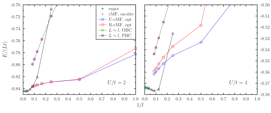
Figure 2: (Color online) Energy per site obtained in cMF calculations on a $L=120$ half-filled periodic 1D lattice at $U/t=2$ (left) and $U/t=4$ (right) as a function of the inverse of the cluster size $l$. $l=1$ R-cMF and U-cMF results correspond to restricted HF and UHF, respectively. We consider cMF results in the on-site basis and with a fully-optimized single-particle basis (opt). They are compared with (exact) calculations on a single cluster (i.e., $L=l$) using open (OBC) and periodic (PBC) boundary conditions. The latter were computed by solving the corresponding Lieb-Wu Lieb and Wu (1968) equations. The energies of $L=l$ calculations with OBC exactly match those of cMF calculations in the full $L=120$ lattice using the on-site basis.

Comparing the results of cMF calculations that include orbital optimization with those in the on-site basis, it is evident that orbital optimization affords a significant improvement in the variational estimate of the ground state energy. In addition, cMF calculations using unrestricted orbitals provide a sizable improvement over the corresponding restricted calculations at $U/t=4$. We note that, at $U/t=4$, cMF calculations do not converge (in $1/l$) as fast to the $L=120$ limit as calculations using PBC, though the former have the advantage of being variational. On the other hand, at $U/t=2$ cMF provides better estimates than $L=l$ calculations for $l<12$, suggesting that a finite-size extrapolation with cMF results should be preferred. We emphasize the significance of this given that, for arbitrary systems, an exact diagonalization can currently only be performed up to lattices of size $18$ or so. A linear extrapolation in $1/l$ of U-cMF energies (using the $l=8$, 10, and 12 results) yield the following estimates in the $l\to L=120$ limit for the ground state energy $E/(Lt)$: $-0.5709(2)$ and $-0.8414(2)$ for $U/t=4$ and 2, respectively. These can be compared with the exact energies of $-0.5738$ and $-0.8444$.

We will often refer to the fraction of correlation energy in assessing the quality of the ground state energy. The correlation energy is here defined as

$$E_{\textrm{corr}}=E_{\textrm{exact}}-E_{\textrm{UHF}},$$ (35)

i.e., the difference between the exact and the UHF energies. (Note that this differs from the traditional quantum chemistry definition based on restricted HF Löwdin (1955).) Figure 3 shows the fraction of correlation recovered in R-cMF and U-cMF calculations using clusters of increasing size ($l=2$ to $l=12$) as a function of $U/t$. The inset shows $-E_{\textrm{corr}}/(Lt)$ as a function of $U/t$. The latter peaks at $\approx 0.1$ at $U/t=4$.

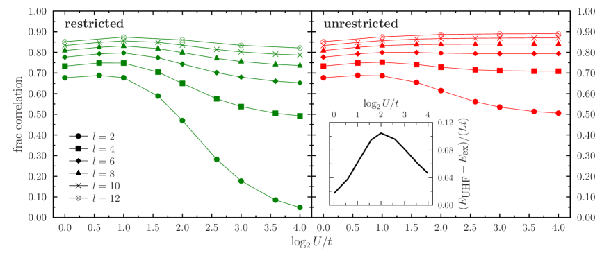
Figure 3: (Color online) Fraction of correlation (with respect to UHF) recovered in restricted (left) and unrestricted (right) cMF calculations in a $L=120$ periodic 1D lattice, as a function of $U/t$. (A log-2 scale is used in $U/t$ for clarity purposes; results are shown from $U/t=1$ to $16$.) Cluster sizes from 2 to 12 were used. The inset in the right panel shows the total correlation energy per site, as a function of $U/t$.

The fraction of correlation in restricted calculations using $l=2$ seems to vanish at large $U/t$, indicating that the Heisenberg limit predicted by this method is roughly the same as the UHF limit. This is not the case in unrestricted $l=2$ calculations, which still recover around $50\,\%$ of the correlation in the large $U/t$ limit. As $l$ becomes larger, the difference between restricted and unrestricted calculations gets smaller, as expected. U-cMF calculations with $l=12$ are able to recover $85$ to $90\,\%$ of the correlation energy across the entire $U/t$ domain plotted, which spans both the weak and the strongly-correlated regimes. Accordingly, the maximum error in the energy per site in $l=12$ U-cMF calculations is about $0.01\,t$ at $U/t=4$, which is remarkable given the simplicity of the approach.

Figure 4 displays the fraction of correlation recovered in U-cMF and U-cPT2 calculations; results are compared with UMP2 and UCCSD. U-cPT2 energies significantly improve over U-cMF results for small cluster sizes. For instance, with $l=2$ U-cPT2 recovers $90\,\%$ ($>75\,\%$) of the correlation energy at small (large) $U/t$. Notice also that U-cPT2 results do not overly deteriorate for large $U/t$ as UMP2 does. UCCSD and U-cPT2 ($l=6$) recover $\gtrapprox 90\,\%$ of the correlation energy across the entire $U/t$. It is interesting to point out that at $U/t=1$ UMP2 and UCCSD results are better than U-cPT2 results with even $l$; U-cPT2 results with odd $l$, on the other hand, slightly overshoot the exact result. Unfortunately, the steep computational scaling of U-cPT2 rendered calculations with $l>6$ as too expensive with our current implementation.

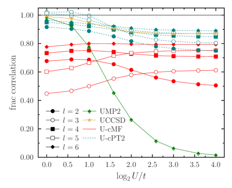
Figure 4: (Color online) Fraction of correlation (with respect to UHF) recovered in unrestricted cMF and cPT2 calculations in a $L=120$ periodic 1D lattice as a function of $U/t$. UMP2 and UCCSD results are provided for comparison purposes.

Figure 5 displays the spectrum of a single cluster Hamiltonian in U-cMF calculations, using cluster sizes of 2, 4, and 6. As PBC are used along with a uniform tiling scheme, all clusters end up displaying identical spectra, although we emphasize that this was not imposed. The eigenvalues are shown in Fig. 5 according to the $n_{\uparrow}$ and $n_{\downarrow}$ quantum numbers within the cluster, reference to the half-filled case. Here, the ground state in the $(0,0)$ sector of each cluster is used to construct the cMF state $|\Phi_{0}\rangle$. Although not shown in the figure, the spectrum should resemble, as $l$ becomes larger, that of a lattice of $l$ sites with OBC to the extent that orbitals remain fully localized. If $\epsilon_{0}^{(x,y)}$ denotes the ground state in the $(x,y)$ sector, the perturbation series is stable (i.e., all denominators are positive) as long as the following conditions are met (we indicate in parenthesis the relevant interactions):

1. the $(0,0)$ sector is gapped (two-cluster dispersion),

2. $2\epsilon_{0}^{(0,0)}<\epsilon_{0}^{(+1,0)}+\epsilon_{0}^{(-1,0)}$ (charge-transfer),

3. $2\epsilon_{0}^{(0,0)}<\epsilon_{0}^{(+1,-1)}+\epsilon_{0}^{(-1,+1)}$ (spin-flip),

4. $2\epsilon_{0}^{(0,0)}<\epsilon_{0}^{(+1,+1)}+\epsilon_{0}^{(-1,-1)}$ (2 clusters, two-electron charge-transfer).

All the conditions are met in the cases plotted in Fig. 5, although as $l$ becomes larger, $2\epsilon_{0}^{(0,0)}\approx\epsilon_{0}^{(+1,-1)}+\epsilon_{0}^{(-1,+1)}$.

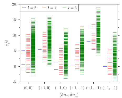
Figure 5: (Color online) Spectrum of the cluster Hamiltonian $\hat{H}^{0}_{c}$ in U-cMF calculations on a half-filled 1D lattice at $U/t=4$, using cluster sizes of 2, 4, and 6. All clusters in the $L=120$ lattice display an identical spectrum. The eigenvalues are classified according to the $n_{\uparrow}$ and $n_{\downarrow}$ quantum numbers within the cluster. Here, $(0,0)$ corresponds to a half-filled cluster, with $l/2$ $\uparrow$- and $\downarrow$-electrons. Only those Hilbert sectors relevant to the evaluation of the second-order energy are shown. (Certain Hilbert sectors are missing as their spectrum is identical to one that is actually displayed; e.g., the $(+1,0)$ and $(0,+1)$ spectra are equivalent, and so are the $(+1,-1)$ and $(-1,+1)$.)

We show in Fig. 6 the contributions of different channels to the second-order energy in U-cPT2 calculations as a function of $U/t$. Results from Fig. 6 indicate that two-cluster spin-flip (two neighboring clusters undergoing a spin flip) and two-cluster 1-electron charge transfer (two clusters interchanging a single electron) processes are the most important contributors to the second-order energy. Beyond that, the remaining two- and three-cluster interactions are small but non-negligible for $U/t<4$. Four-cluster interactions are very small across all $U/t$.

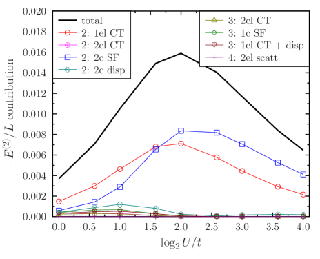
Figure 6: (Color online) Contributions to the second-order energy in U-cPT2 calculations ($L=120$ 1D periodic lattice) using a cluster size of 4 as a function of $U/t$. The notation used in the key takes the form “# clusters: interaction type”. Here, CT stands for charge transfer and SF refers to spin flip. The interaction channels are those from Tab. 1; two-electron charge transfer processes are of opposite spin due to the nature of the Hubbard interaction.

We now turn our attention to the spin-spin correlations in the ground state. As the cMF ansatz breaks the translational invariance of the Hubbard model, we have computed averaged spin-spin correlations, defined by

$$\bar{S}(\mathbf{j})=\frac{1}{L}\sum_{\mathbf{j^{\prime}}}\langle\mathbf{S}_{\mathbf{j^{\prime}}}\cdot\mathbf{S}_{\mathbf{j}-\mathbf{j^{\prime}}}\rangle,$$ (36)

where $\mathbf{j}$ labels a lattice site. We plot in Fig. 7 the (real-space) spin-spin correlations obtained from R-cMF and U-cMF calculations at $U/t=4$.

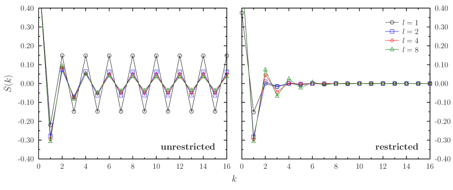
Figure 7: (Color online) Real-space spin-spin correlations computed from unrestricted (left) and restricted (right) optimized cMF states for a $L=120$ periodic 1D lattice at $U/t=4$. The $l=1$ result in the left panel corresponds to UHF, while that in the right panel corresponds to restricted HF (i.e., a product of plane-wave states).

It becomes evident that unrestricted calculations (left panel) yield a structure with long range order. R-cMF, on the other hand, has non-vanishing spin-spin correlations only within the cluster; inter-cluster correlations vanish due to the spin singlet character of each cluster state. The long range spin-spin correlations in U-CMF are systematically decreased as the size of the cluster is increased. In the short range, both R-cMF and U-cMF yield significant corrections to RHF and UHF, respectively. With $l=8$, R-cMF and U-cMF display similar correlations to the first few neighbors (small $k$), with hints of the $1/k$ decay Imada et al. (1992); Essler et al. (2005) present in the exact solution at long range.

A cleaner picture of the spin-spin correlations can be obtained by looking at them in reciprocal space. Figure 8 displays the (discrete) Fourier-transformed spin-spin correlations, at wave-vectors $q=0$ and $q=\pi$, obtained from R-cMF and U-cMF calculations. (R-cMF results at $q=0$ are not shown as they identically vanish.) The two momenta are the most relevant ones: the $q=0$ result provides $\langle\hat{S}^{2}\rangle$, which should identically vanish for a spin singlet, while $q=\pi$ provides the anti-ferromagnetic structure factor. We see that both values are significantly decreased in U-cMF with respect to what UHF predicts. Note that both R-cMF and U-cMF should converge to the same value (the exact one) as $l$ tends to the $L=120$ limit.

Figure 8: (Color online) Fourier-transformed averaged spin-spin correlations ($L=120$ 1D periodic lattice at $U/t=4$) in U-cMF and R-cMF calculations as a function of the inverse of the cluster size. Two $q$ values are plotted, namely 0 and $\pi$ (note that the $q=0$ curve is enhanced by a factor of 50 for clarity purposes). U-cMF and R-cMF calculations should tend to the same $q=\pi$ finite value as $l\to L$. The $l\to L$ limit at $q=0$ of U-cMF results should be 0 as the exact ground state corresponds to a true singlet state.

IV.3 2D: half-filling

We now consider the periodic two-dimensional, half-filled square lattice. All the calculations in this section use a $12\times 12$ periodic lattice, which should provide near-thermodynamic limit estimates for $U/t\geq 2$. In 2D, we are able to find a plethora of local minima (with respect to orbital rotations and coefficients in the cMF expansion) corresponding to different (approximate) tiling patterns. In principle, one could argue that, given a fixed number of clusters with their associated quantum numbers ($n_{\uparrow}$, $n_{\downarrow}$), an optimal solution (a global minimum) exists which minimizes the energy. We did not attempt to locate it but we did consider several uniform-like patterns that converge to different local minima.

We show in Fig. 9 the tiling patterns adopted in U-cMF calculations on the $12\times 12$ lattice. A label used to identify each pattern is also provided in the figure. In most of the tilings displayed, a staggered configuration was chosen over an otherwise uniform tiling as it leads to lower variational energies. A staggered dimer configuration is used in clusters of size 2. For clusters of size 4, we discuss results with a square-based (staggered, $\mathbf{4_{S}}$) tiling and a z-shaped ($\mathbf{4_{Z}}$) tiling. We have considered a staggered configuration in terms of slabs ($\mathbf{6_{S1}}$) and hats ($\mathbf{6_{H1}}$) in connection with clusters of size 6. Clusters of size 8 with a staggered slab ($4\times 2$, $\mathbf{8_{S}}$) and a z-shaped ($\mathbf{8_{Z}}$) configuration are used, which can be thought of as simple dimers of the considered size-4 clusters. We finally also examined staggered plaquette configurations with clusters of size 9 and 12.

We should point that, in constrast to Ref. Isaev et al., 2009, all the considered tiling patterns lead to a qualitatively correct description of the ground state character, i.e., all structures lead to a ground state density with non-zero magnetization in a Néel-type configuration. This is because the ground state of each cluster was independently optimized, without requiring that all the clusters share the same ground state.

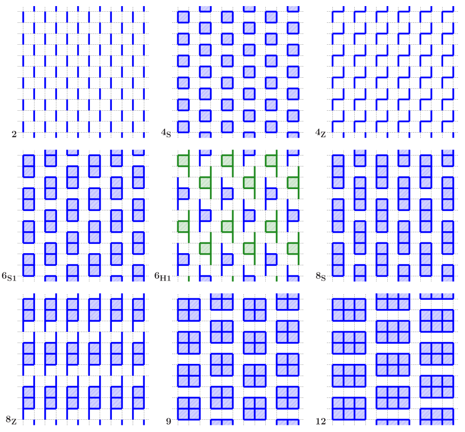
Figure 9: (Color online) Tiling patterns adopted in U-cMF calculations on a square $12\times 12$ periodic 2D square lattice at half-filling. Sites within the same cluster are connected by solid lines; fully enclosed regions are shaded. A key is provided to the left of each structure.

The left panel of Fig. 10 shows the correlation energy (divided by the UHF energy) predicted by U-cMF as a function of $U/t$. (These can be contrasted with auxiliary-field quantum Monte Carlo (AFQMC) results shown in Fig. 13.) Here, size-12 U-cMF predicts that the correlation energy is $\approx 1.5\,\%$ ($\approx 10\,\%$) of the UHF energy at $U/t=2$ ($U/t=16$). Large differences in the correlation energy predicted are observed as the clusters get larger, particularly at large $U/t$, which is unsurprising. A larger cluster, irrespective of its shape, tends to yield a larger correlation energy than a smaller one, but a few exceptions are observed. When clusters of the same size are compared in different tiling schemes (e.g., $\mathbf{4_{S}}$ and $\mathbf{4_{Z}}$), we observe that the more compact the cluster is, the better the variational estimate for the ground state energy becomes at large $U/t$. Thus, the square tiling pattern in size-4 clusters yields a larger correlation energy than the z-shaped one.

The right panel of Fig. 10 shows the difference between the double occupancy ($D=\sum_{i}\langle n_{i\uparrow}n_{i\downarrow}\rangle$) per site predicted in U-cMF calculations with respect to that of UHF (which is shown in the inset). UHF overestimates (underestimates) the double occupancy at small (large) $U/t$. A relatively systematic improvement is observed in the double occupancy as the cluster becomes bigger.

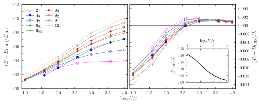
Figure 10: (Color online) (Left) Correlation energy (with respect to UHF), divided by the UHF energy, recovered in U-cMF calculations in a $12\times 12$ periodic 2D square lattice, as a function of $U/t$. The tiling patterns considered are those displayed in Fig. 9. (Right) Difference with respect to the double occupancy per site predicted by UHF in a variety of U-cMF calculations in a $12\times 12$ periodic square lattice. The double occupancy of UHF itself is shown in the inset.

To show that other tiling patterns do not lead to fundamentally different results, we show in Fig. 11 the correlation energy predicted in U-cMF calculations with different tiling schemes using clusters of size 6. The additional tiling schemes (aside from those in Fig. 9) are shown in Fig. 12. Several of them lead to approximately the same ground state energies. As previously discussed, the more compact the clusters are, the better the variational estimate of the ground state energy at large $U/t$. The same may not be true at small $U/t$. For instance, the lowest energies obtained at $U/t=2$ corresponded to structure $\mathbf{6_{Z}}$.

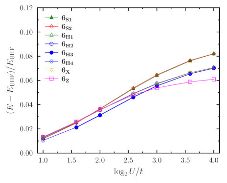
Figure 11: (Color online) Same as Fig. 10. Different tiling patterns with clusters of size 6 (cf. Figs. 9 and 12) are displayed.

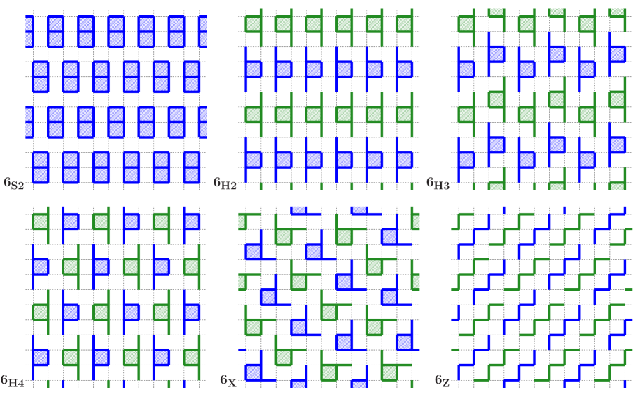
Figure 12: (Color online) Some additional tiling patterns (with clusters of size 6) adopted in U-cMF calculations on a square $12\times 12$ periodic 2D square lattice at half-filling.

We show in Fig. 13 the ground state correlation energies, divided over the UHF energy, obtained from U-cMF and U-cPT2 calculations as a function of $U/t$. Results are compared with UMP2, UCCSD, and AFQMC LeBlanc et al. (2015), which can be deemed as numerically exact at half-filling. UMP2 displays the same behavior observed in 1D, with the correlation energy vanishing for large $U/t$. It is evident that the U-cMF results are not competitive with UCCSD or AFQMC, even with the larger clusters from Fig. 10. For instance, U-cMF using structure $\mathbf{6_{S1}}$ recovers $<50\,\%$ of the correlation energy across all $U/t$. On the other hand, U-cPT2 provides a sizable improvement over U-cMF results, with structure $\mathbf{6_{S1}}$ capturing $\approx 85\,\%$ of the correlation energy at $U/t=12$. This is not far from UCCSD, which recovers $\approx 90\,\%$ of the correlation energy predicted by AFQMC at $U/t=12$. (Finite size effects account for most of the difference between UCCSD and AFQMC at $U/t=2$.)

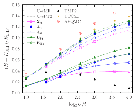
Figure 13: (Color online) Same as Fig. 10. U-cMF and U-cPT2 calculations are compared with UMP2, UCCSD and AFQMC. AFQMC results, from Ref. LeBlanc et al., 2015, correspond to thermodynamic limit estimates.

Figure 14 displays the (discrete) Fourier-transformed averaged spin-spin correlations, at wave-vectors $\mathbf{q}=(0,0)$ and $\mathbf{q}=(\pi,\pi)$, obtained from U-cMF calculations at $U/t=8$ in the 2D lattice. As it was done in the 1D case, the spin-spin correlations are averaged as the wavefunction ansatz breaks the translational invariance of the lattice. It becomes evident that as the cluster becomes bigger (regardless of the specific tiling pattern), the spin-spin correlations get reduced with respect to UHF. In particular, large clusters display less than half the spin-contamination per-site (i.e., the deviation of $\bar{\mathcal{S}}(0,0)$ from 0) of UHF. The anti-ferromagnetic structure factor is also reduced, though this should converge to a finite value in the limit $l\to L$.

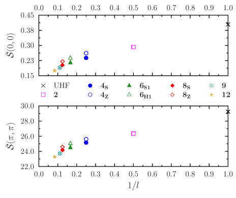
Figure 14: (Color online) Fourier-transformed averaged spin-spin correlations ($12\times 12$ periodic 2D square lattice at $U/t=8$) in U-cMF calculations as a function of the inverse of the cluster size. UHF ($l=1$) results are also displayed. Two $\mathbf{q}$ values are plotted, namely $(0,0)$ and $(\pi,\pi)$.

IV.4 2D: lightly-doped regime

In the 2D lightly-doped regime, we considered periodic square lattices with $\langle n\rangle=0.8$ and $\langle n\rangle=0.875$, following Ref. LeBlanc et al., 2015. We have used a $10\times 10$ lattice for the former case and a $16\times 8$ lattice for the latter case in order to have a lattice commensurate with the striped order expected to develop, as described below.

Xu et al. Xu et al. (2011) discussed the UHF phase diagram for the 2D Hubbard model in the half-filled and lightly-doped regime. For $\langle n\rangle\gtrapprox 0.9$, the system transitions from a paramagnetic to a linear spin density wave regime at $U/t\approx 1$ (cf. Fig. 17 in Ref. Xu et al., 2011). A phase transition to a regime with diagonal spin density wave character occurs at $U/t\approx 4$. Finally, the system becomes ferromagnetic at large $U/t$. This UHF description has guided our U-cMF calculations.

IV.4.1 $\langle n\rangle=0.8$

We show in Fig. 15 the spin and hole density profiles of UHF solutions with linear and diagonal spin density wave character. The (approximate) tiling pattern adopted in U-cMF calculations is superimposed in the figure. Clusters of size 6 with 4 electrons (2 $\uparrow$ and 2 $\downarrow$) have been used to describe the sectors with high hole density. On the other hand, the remaining regions with Néel character have been described in terms of a staggered dimer configuration in structures ${\mathbf{1}}l$ and ${\mathbf{1}}d$, corresponding to the linear and diagonal spin wave character, respectively. In ${\mathbf{2}}l$ and ${\mathbf{2}}d$, the dimers have been combined into half-filled clusters of size 4 as depicted in Fig. 15.

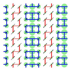
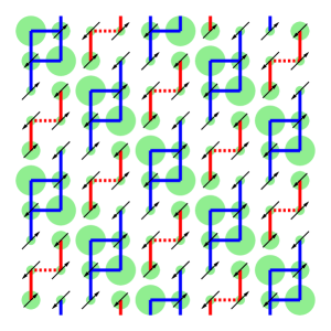
Figure 15: (Color online) Hole and spin density profiles of UHF solutions ($10\times 10$ periodic lattice, $\langle n\rangle=0.8$) obtained at $U/t=8$ with linear (left) and diagonal (right) spin density wave character. The magnitude of the hole density is proportional to the area of the green circles. The magnitude of the spin density is proportional to the size of the arrows. Superimposed on them we display the tiling patterns adopted in U-cMF calculations. Clusters with 6 orbitals and 4 electrons (solid blue) have been used in the high hole density sectors, while the Néel regions are described in terms of staggered dimers (solid red); this leads to structures ${\mathbf{1}}l$ and ${\mathbf{1}}d$, respectively, for linear and diagonal order. We have additionally considered a tiling pattern where the staggered dimers are combined into size 4-clusters, following the dotted lines, leading to structures ${\mathbf{2}}l$ and ${\mathbf{2}}d$.

The resulting spin- and charge-density profiles obtained from U-cMF calculations with structures ${\mathbf{1}}l$ and ${\mathbf{1}}d$ are displayed in Fig. 16. The profiles resemble closely those obtained from UHF itself and shown in Fig. 15. The main difference is the partial shift of the hole density away from the main stripes into the neighboring sites. This suggests that the hole density is too localized in the UHF solution.

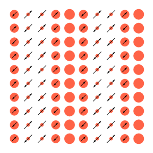
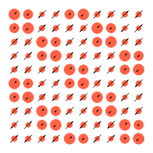
Figure 16: (Color online) Hole and spin density profiles from U-cMF calculations ($10\times 10$ lattice, $\langle n\rangle=0.8$) at $U/t=8$ with linear (left, ${\mathbf{1}}l$) and diagonal (right, ${\mathbf{1}}d$) ordering. The magnitude of the hole density is proportional to the area of the red circles. The magnitude of the spin density is proportional to the size of the arrows.

We show in Tab. 2 the resulting ground state energies from U-cMF and U-cPT2 calculations. Results are compared with UHF, UMP2, UCCSD, and density matrix embedding (DMET) calculations Zheng and Chan (2015), which can be deemed as highly accurate. U-cMF provides a significant improvement over UHF energies, indicating the inaccurate treatment of short-range correlations in the simple HF description. The error in the UHF energies becomes very significant ($>0.2\,t$) at large $U/t$, sizably larger than the error in the half-filled regime. Interestingly, the linear spin density wave character is favored in U-cMF even at relatively large $U/t$. We cannot rule out, nevertheless, that this is an artifact of the particular tiling pattern chosen. The use of the size-4 clusters in place of the Néel dimers in U-cMF provides an improvement of about $10^{-3}\,t$ in the ground state energy for all $U/t$ values quoted.

Table 2: Ground state energies predicted with a variety of methods for a Hubbard 2D periodic $10\times 10$ lattice with $\langle n\rangle=0.8$.

method	$U=2t$	$U=4t$	$U=6t$	$U=8t$	$U=12t$
DMET	$-1.3062(4)$	$-1.108(2)$	$-0.977(4)$	$-0.88(3)$
UHF (diag)	$-1.2165$	$-0.9646$	$-0.7933$	$-0.6815$	$-0.5501$
UHF (linear)	$-1.2678$	$-0.9774$	$-0.7843$	$-0.6597$
UMP2	$-1.3114$	$-1.0760$	$-0.8832$	$-0.7767$
UCCSD	$-1.3094$	$-1.0925$	$-0.9208$	$-0.8246$
UCCSD(T)	$-1.3108$	$-1.1045$	$-0.9357$	$-0.8444$
U-cMF(${\mathbf{1}}d$)			$-0.8417$	$-0.7396$
U-cMF(${\mathbf{2}}d$)			$-0.8429$	$-0.7406$
U-cMF(${\mathbf{1}}l$)		$-1.0217$	$-0.8520$	$-0.7460$	$-0.6271$
U-cMF(${\mathbf{2}}l$)		$-1.0227$	$-0.8536$	$-0.7478$	$-0.6288$
U-cPT2(${\mathbf{1}}l$)		$-1.0865$	$-0.9380$	$-0.8450$	$-0.7394$
U-cPT2(${\mathbf{2}}l$)		$-1.0889$	$-0.9435$	$-0.8526$	$-0.7513$

Second-order PT provides a significant improvement over mean-field energies (both in HF and cMF). The UMP2 results are, however, far from UCCSD at large $U/t$. The difference between UCCSD(T) and UCCSD is also large in the strongly-correlated regime, indicating the necessity of going beyond double excitations in the coupled-cluster ansatz. This is also evident by comparing UCCSD and DMET results. U-cPT2(${\mathbf{2}}l$) is competitive with UCCSD at $U/t=4$ but outperforms even UCCSD(T) in the large $U/t$ regime.

IV.4.2 $\langle n\rangle=0.875$

We now turn our attention to even lighter doping, namely $\langle n\rangle=0.875$. We show in Fig. 17 the spin and hole density profiles of UHF solutions with linear and diagonal spin density wave character. Note that kinks are needed in a $16\times 8$ lattice in the diagonal density wave profile; only a much larger $16\times 16$ lattice is commensurate with a fully diagonal profile. The (approximate) tiling pattern adopted in U-cMF calculations (with a linear density wave character) is superimposed in the figure. As we did previously in the $10\times 10$ lattice, the regions with Néel character have been described in terms of a staggered dimer configuration (structure $\mathbf{1}$), while the regions of high hole density are tiled into clusters of size 6 (with 2 $\uparrow$- and 2 $\downarrow$-electrons each). The Néel dimers have been combined into half-filled clusters of size 6 and 4 in structure $\mathbf{2}$, following the pattern indicated in Fig. 17.

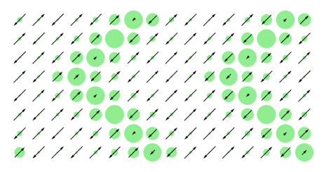
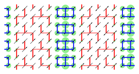
Figure 17: (Color online) Hole and spin density profiles of UHF solutions ($16\times 8$ periodic lattice, $\langle n\rangle=0.875$) obtained at $U/t=8$ with diagonal (top) and linear (bottom) spin density wave character. The magnitude of the hole density is proportional to the area of the green circles. The magnitude of the spin density is proportional to the size of the arrows. Superimposed on the bottom scheme we display the tiling pattern adopted in U-cMF calculations. The Néel regions are described in terms of staggered dimers (solid red), leading to structure $\mathbf{1}$, while regions of high hole density are described with slab-shaped clusters of size 6 (solid blue). We have also considered a pattern (structure $\mathbf{2}$) where the dimers are combined into half-filled clusters of size 6 and 4, following the dotted lines.

Table 3 shows the ground state energies obtained from U-cMF and U-cPT2 calculations. Results are compared with UHF, UMP2, UCCSD, and DMET. Just as in the $\langle n\rangle=0.8$ case, U-cMF improves significantly over UHF. It remains true that second-order PT provides a nice refinement on top of the mean-field result. The triples correction in UCCSD(T) becomes significant at large $U/t$, signaling the deficiencies in UCCSD. U-cPT2 is a bit shy of UCCSD quality at $U/t=4$, but becomes competitive with UCCSD(T) at $U/t=8$.

Table 3: Ground state energies predicted with a variety of methods for a Hubbard 2D periodic $16\times 8$ lattice with $\langle n\rangle=0.875$.

method	$U=2t$	$U=4t$	$U=6t$	$U=8t$	$U=12t$
DMET	$-1.2721(6)$	$-1.031(3)$	$-0.86(1)$
UHF (diag)			$-0.7184$	$-0.6008$	$-0.4682$
UHF (linear)	$-1.2270$	$-0.9109$	$-0.7128$
UMP2	$-1.2732$	$-0.9858$	$-0.7833$	$-0.6594$
UCCSD	$-1.2719$	$-1.0093$	$-0.8305$	$-0.7147$
UCCSD(T)	$-1.2738$	$-1.0195$	$-0.8446$	$-0.7299$
U-cMF(${\mathbf{1}}$)		$-0.9476$	$-0.7633$	$-0.6477$	$-0.5176$
U-cMF(${\mathbf{2}}$)		$-0.9500$	$-0.7667$	$-0.6514$	$-0.5210$
U-cPT2(${\mathbf{1}}$)		$-1.0004$	$-0.8289$	$-0.7204$	$-0.5965$
U-cPT2(${\mathbf{2}}$)		$-1.0040$	$-0.8347$	$-0.7276$	$-0.6068$

Figures 18 and 19 depict the Fourier-transformed spin-spin and density-density correlations obtained from U-cMF calculations (using structure $\mathbf{1}$). Just as in the case of 1D, we have performed a global average over sites in order to remove the expected fluctuations due to the (spatial) symmetry broken character of the ansatz. The spin-spin correlations show a maximum at $\mathbf{q}=(7\pi/8,\pi)$ which becomes more intense as $U/t$ is increased from 4 to 8. The density-density correlations display their maximum at $\mathbf{q}=(\pi/4,0)$. These observed profiles are consistent with the linear spin density wave character of the UHF charge and spin densities. Symmetry-projected calculations in Refs. Rodríguez-Guzmán et al., 2014; Juillet and Frésard, 2013 also show the same features. We refer the reader to Ref. Chang and Zhang, 2010 for a discussion of the emergence of spin and charge order in the doped Hubbard model.

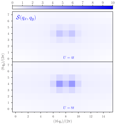
Figure 18: (Color online) Fourier-transform $\bar{\mathcal{S}}(q_{x},q_{y})$ of the averaged spin-spin correlations obtained from U-cMF (structure ${\mathbf{1}}$) calculations in a $16\times 8$ ($\langle n\rangle=0.875$) lattice at $U/t=4$ (top) and $U/t=8$ (bottom).

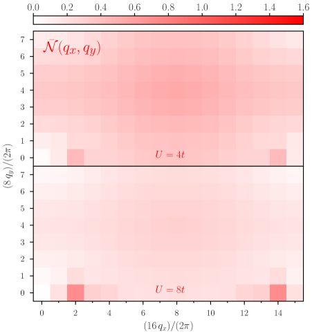
Figure 19: (Color online) Fourier-transform $\bar{\mathcal{N}}(q_{x},q_{y})$ of the averaged density-density correlations obtained from U-cMF (structure ${\mathbf{1}}$) calculations in a $16\times 8$ ($\langle n\rangle=0.875$) lattice at $U/t=4$ (top) and $U/t=8$ (bottom). The strong peak at $(0,0)$ ($=N^{2}/L$) has been removed for clarity purposes.

V Discussion

In Sec. II, we have described the cluster mean-field approach to treat strongly-correlated fermionic systems. A cMF state (including the orbital optimization degrees of freedom) is used as a variational ansatz for the ground state wavefunction. This, by construction, is guaranteed to provide better variational estimates than HF when the size of the cluster (assuming uniform tiling) is larger than 1. Because of the simple nature of the ansatz, a RS-PT scheme can be adopted to account for the missing inter-cluster correlations. The results presented in Secs. IV.2, IV.3, and IV.4 provide evidence that a cluster-based approach can provide a (semi)-quantitative description of the ground state of the half-filled 1D and 2D Hubbard models, as well as for the lightly-doped regime in 2D square lattices.

In the half-filled 1D model, results with comparable accuracy to UCCSD can be obtained by U-cMF using a sufficiently large cluster or by using U-cPT2 with smaller cluster sizes. Not only the energy is improved in U-cMF with respect to UHF, but also other ground state properties such as spin-spin correlations. Due to the local nature of the interactions in the Hubbard Hamiltonian, contributions to the second-order energy arise mostly from two-cluster (spin flip and one-electron charge transfer) interactions.

In the half-filled 2D square model, U-cMF was not as accurate as it was in the 1D case, even when using clusters of size 12. This difference can be understood in terms of the missing inter-cluster correlations and the area-law of entanglement entropy Eisert et al. (2010). Whereas in 1D the size of the boundary (which determines the missing inter-cluster correlations) of a given cluster remains fixed, in 2D it scales as the perimeter of the cluster itself. This also explains why more tightly packed clusters provide better energetic variational estimates for large $U/t$, as the clusters become more localized. A significant improvement to the ground state energy is obtained with U-cPT2, where results are again comparable (although slightly poorer) than UCCSD.

In the lightly-doped regime, we have used ad hoc tiling schemes that mostly respect the underlying spin density wave profile obtained with UHF. Following this strategy, results will be relevant to the extent that UHF itself provides a qualitatively correct description of the character of the ground state. Our calculations suggest that it does. U-cMF results provide a sizable improvement over the UHF description and U-cPT2 results are competitive with UCCSD at small $U/t$ and with UCCSD(T) at large $U/t$. The predicted U-cPT2 energies are still above the DMET estimates, indicating that part of the long-range correlations expected to develop in the lightly-doped regime are still unaccounted for. These may be described with higher order RS-PT or other more powerful many-body approaches.

We note that it is generally true that describing inter-cluster correlations (here via second-order RS-PT) improves the ground state energy to a larger extent than enlarging the size of the cluster in mean-field calculations. (A clear exception to this is the fact that U-cMF with a cluster of size 2 provides better results at large $U/t$ than UMP2.) The good quality of U-cPT2 results suggest that the renormalized Hamiltonian (expressed in terms of cluster states) is more amenable to a perturbative treatment than in the case of the HF particle-hole transformation. Thus traditional many-body approaches (such as second-order RS-PT) can be built on top of the cluster mean-field description to provide a high quality answer. This is further explored in Appendix A, were we show the results of high-order RS-PT calculations in a small lattice. In the remainder of this section we discuss possible strategies that can improve the results presented in this manuscript.

Perhaps the simplest strategy is to increase the flexibility in the mean-field variational ansatz, which can be done in a variety of ways. The full Hilbert space (i.e., not restricted to a given $m_{s}$ sector) or, in fact, the full even- or odd-number parity Fock space within each cluster can be used. In doing this, it is not necessary to use a more general form for the single-particle transformation that defines the orbital optimization. The latter can be done in addition to (or in place of). Thus in systems where local number fluctuations are essential, a Bogoliubov-de Gennes single-particle transformation can be used.

The local character of the clusters can be exploited in cPT2 calculations by, e.g., truncating the computed interactions according to some distance criterion. This could alleviate significantly the computational cost in cPT2 calculations (bringing them to linear scaling in the number of clusters) while also facilitating carrying out the cPT$n$ expansion to a higher order. In order to deal with the large number of interacting clusters and states, a stochastic sampling of contributing processes can be performed.

At this point, we would like to comment on the nature of the states used to carry out the perturbation expansion. In this work, we have used an energy criterion to truncate the number of cluster states when this was imperative. Other criteria may be used, such as a density matrix based criterion (akin to the one used in DMRG White (1992, 1993)). Here, one would diagonalize the Hamiltonian of the cluster interacting with part of its environment. The resulting ground state wavefunction is projected into the cluster states; those states with highest occupation constitute the optimal subset of states to use. Our main concern regarding this strategy is that the resulting cluster + (relevant) environment may become too large to solve (exactly) for its ground state. For instance, the environment around a four-site square cluster in a 2D lattice should include at least eight additional sites/orbitals.

Of course, other strategies to account for inter-cluster correlations may be used. One possible alternative in the case where there are a few nearly degenerate states in each cluster, is to diagonalize the full Hamiltonian in the direct product basis spanned by the relevant cluster states. This is part of the essence of the contractor renormalization group (CORE) algorithm Morningstar and Weinstein (1996); Capponi et al. (2004); Siu and Weinstein (2007) and has also been used in the active space decomposition (ASD) Parker et al. (2013); Parker and Shiozaki (2014) method in quantum chemistry.

We think a coupled-cluster based approach such as the one proposed by Li in BCCC Li (2004) is among the most promising avenues. In particular, a coupled-cluster ansatz should provide an improved description of the missing inter-cluster correlations in the mean field than low-order RS-PT. Given that the cluster-based Hamiltonian contains up to four-tile interactions, it appears that the minimal coupled-cluster model should include up to quadruple excitations. Nevertheless, we have observed that two-tile interactions dominate the contribution to the second-order energy. It may not be unreasonable to restrict the excitation to singles and doubles. Moreover, locality can also be exploited within a coupled-cluster framework.

Lastly, we would like to point out that even though we have used the cMF approach to study strongly interacting systems, it may be used in other contexts. In particular, systems which can be effectively represented in terms of weakly interacting fragments of otherwise strongly-correlated fermions (see Appendix B) can be very efficiently described by low-order perturbation theory based on a cMF state.

VI Conclusions

We have introduced a cluster mean-field variational approach and discussed its applicability to describe the ground state of strongly-correlated fermion systems. In this work, the full optimization of the cluster mean-field state has been carried out, including orbital optimization, with the restriction that the cluster state has well-defined $n$ and $m_{s}$ quantum numbers. The restrictions are imposed in order to preserve $N$ and $M_{s}$ in the full system. The cluster product state constitutes an eigenstate of a mean-field (zero-th order) Hamiltonian, which allows us to formulate a RS perturbative approach to improve upon the mean-field description.

We have presented mean-field and second-order perturbative results of the ground state energies (and other observables) of the periodic 1D and square 2D Hubbard models. In the half-filled 1D case, our U-cMF results become as accurate as UCCSD across all $U/t$ for sufficiently large clusters. U-cPT2 results on smaller clusters also provide a consistent description across all interaction strengths. In 2D at half-filling, U-cMF is poorer than in the 1D case yet U-cPT2 provides ground state energies of near UCCSD quality. In the lightly-doped regime of the 2D model, U-cPT2 results remain competitive with UCCSD although they are still not competitive with DMET estimates. In general, we observe that U-cPT2 energies with small clusters are often better than U-cMF results with significantly larger ones.

Overall, the results of this work suggest that a cluster mean-field approach can provide an excellent starting point and a path to a highly accurate, efficient description of strongly-correlated fermionic systems, and the Hubbard model in particular. Several strategies to improve the mean-field description as well as correlated approaches built on top of it have been suggested.

Appendix A High-order perturbation theory

For sufficiently small systems, the standard RS perturbation series can be evaluated to high order by direct solution of the RS-PT equations

$$(\hat{H}_{0}-E^{(0)})|\Psi^{(m)}\rangle= \,\hat{V}|\Psi^{(m-1)}\rangle-\sum_{l=0}^{m-1}E^{(m-l)}|\Psi^{(l)}\rangle,$$ (37)

$$E^{(m)}= \,\langle\Psi^{(0)}|\hat{V}|\Psi^{(m-1)}\rangle,$$ (38)

where we have assumed intermediate normalization ($\langle\Psi^{(0)}|\Psi^{(m)}\rangle=0\quad\forall\quad m>0$). We have evaluated the UMP$n$ (i.e., RS-PT using canonical UHF orbitals and orbital energies) and U-cPT$n$ (as formulated in Sec. II, using a cluster of size 2) perturbation series for a half-filled $L=8$ 1D periodic lattice at $U/t=4$ and $U/t=8$. The energy as a function of $n$ is displayed in Fig. 20.

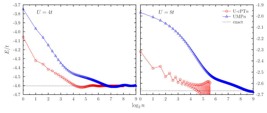
Figure 20: (Color online) Convergence of the UMP$n$ and U-cPT$n$ perturbation series for a half-filled $L=8$ periodic 1D lattice at $U/t=4$ (left) and $U/t=8$ (right). A cluster size of 2 has been used in U-cPT$n$ calculations. The exact ground state energy is denoted by a dashed line. Due to the divergent nature of the U-cPT$n$ series at $U/t=8$, we have truncated at order $n=48$.

The UMP$n$ series approaches the exact energies very slowly, particularly at large $U/t$. On the other hand, U-cPT$n$ is much faster approaching the exact energy, although the series has a divergent nature at $U/t=8$. This is likely due to the near degeneracies expected to appear at large $U/t$ in the spectrum of each cluster. It is possible that a convergent nature can be restored by tweaking the definition of the zero-th order Hamiltonian. In spite of that, these results support the premise that once correlations within the cluster have been described accurately, the ground state of the resulting renormalized Hamiltonian can be expressed by a many-body expansion that is more rapidly convergent than the common UMP$n$ series.

Appendix B Dimerized Hubbard model

Consider a Hubbard lattice tiled into clusters. As the clusters become non-interacting, the cMF approach becomes exact. In this section, we assess the quality of the cMF and cPT2 ground state energies as a function of the interaction between clusters. Being more specific, we consider the dimerized periodic Hubbard 1D model (see, e.g., Ref. Mila and Penc, 1995), given by the Hamiltonian

$$\hat{H}= \,-t_{1}\sum_{\textrm{odd }j,\sigma}(c^{\dagger}_{j+1,\sigma}\,c_{j,\sigma}+\textrm{h.c.})$$

$$\,-t_{2}\sum_{\textrm{even }j,\sigma}(c^{\dagger}_{j+1,\sigma}\,c_{j,\sigma}+\textrm{h.c.})+U\sum_{j}n_{j,\uparrow}\,n_{j,\downarrow}.$$ (39)

Figure 21 shows the UHF, U-cMF, and U-cPT2 ground state energies obtained in a half-filled $L=8$ periodic 1D lattice, as a function of the ratio $t_{2}/t_{1}$ with $U/t_{1}=4$. Clusters of size 2 have been used in cMF and cPT2 calculations.

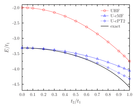
Figure 21: (Color online) UHF, U-cMF, and U-cPT2 ground state energies for a half-filled $L=8$ periodic 1D dimerized Hubbard lattice (cf. Eq. 39) as a function of the ratio $t_{2}/t_{1}$, with $U/t_{1}=4$. U-cMF and U-cPT2 calculations employ clusters of size 2.

At $t_{2}/t_{1}=0$, the exact ground state energy reduces to four-times the energy of an $L=2$ half-filled lattice with OBC. Naturally, U-cMF reproduces this result, while UHF converges to an energy that is equal to four-times the energy of the corresponding UHF result for the $L=2$ lattice. U-cMF (U-cPT2) remains highly accurate up to $t_{2}/t_{1}\approx 0.3$ ($t_{2}/t_{1}\approx 0.6$). On the other hand, U-cMF and U-cPT2 are not nearly as accurate in the vicinity of $t_{2}/t_{1}=1$, yet they still provide sizable improvements over the UHF description. The mean-field approach recovers $\approx 35\,\%$ of the correlation energy, while U-cPT2 is able to capture around $65\,\%$ of it. These results suggest that a simple cluster-based approach can accurately describe weak interactions among otherwise strongly-correlated fragments.

References

- Anderson (1987) P. W. Anderson, Science 235, 1196 (1987).
- McWeeny (1959) R. McWeeny, Proc. R. Soc. Lond. A 253, 242 (1959).
- McWeeny (1960) R. McWeeny, Rev. Mod. Phys. 32, 335 (1960).
- Isaev et al. (2009) L. Isaev, G. Ortiz, and J. Dukelsky, Phys. Rev. B 79, 024409 (2009).
- Zhao et al. (2014) J. Zhao, C. A. Jiménez-Hoyos, G. E. Scuseria, D. Huerga, J. Dukelsky, S. M. A. Rombouts, and G. Ortiz, J. Phys.: Condens. Matter 26, 455601 (2014).
- Schrödinger (1926) E. Schrödinger, Ann. Phys. 385, 437 (1926).
- Li (2004) S. Li, J. Chem. Phys. 120, 5017 (2004).
- Fang et al. (2008) T. Fang, J. Shen, and S. Li, J. Chem. Phys. 128, 224107 (2008).
- Shen and Li (2009) J. Shen and S. Li, J. Chem. Phys. 131, 174101 (2009).
- Xu and Li (2013) E. Xu and S. Li, J. Chem. Phys. 139, 174111 (2013).
- Cirac and Verstraete (2009) J. I. Cirac and F. Verstraete, J. Phys. A.: Math. Theor. 42, 504004 (2009).
- Orús (2014) R. Orús, Ann. Phys. 349, 117 (2014).
- White (1992) S. R. White, Phys. Rev. Lett. 69, 2863 (1992).
- White (1993) S. R. White, Phys. Rev. B 48, 10345 (1993).
- Changlani et al. (2009) H. J. Changlani, J. M. Kinder, C. J. Umrigar, and G. K.-L. Chan, Phys. Rev. B 80, 245116 (2009).
- Mezzacapo et al. (2009) F. Mezzacapo, N. Schuch, M. Boninsegni, and J. I. Cirac, New J. Phys. 11, 083026 (2009).
- Mezzacapo and Cirac (2010) F. Mezzacapo and J. I. Cirac, New J. Phys. 12, 103039 (2010).
- Neuscamman et al. (2011) E. Neuscamman, H. Changlani, J. Kinder, and G. K.-L. Chan, Phys. Rev. B 84, 205132 (2011).
- Hubbard (1963) J. Hubbard, Proc. Roy. Soc. Lond. A 276, 238 (1963).
- Lieb and Wu (1968) E. H. Lieb and F. Y. Wu, Phys. Rev. Lett. 20, 1445 (1968).
- Scalapino (2007) D. Scalapino, in Handbook of High-Temperature Superconductivity, edited by J. R. Schrieffer and J. S. Brooks (Springer New York, 2007) pp. 495–526.
- LeBlanc et al. (2015) J. P. F. LeBlanc, A. E. Antipov, F. Becca, I. W. Bulik, G. K.-L. Chan, C.-M. Chung, Y. Deng, M. Ferrero, T. M. Henderson, C. A. Jiménez-Hoyos, E. Kozik, X.-W. Liu, A. J. Millis, N. V. Prokof’ev, M. Qin, G. E. Scuseria, H. Shi, B. Svistunov, L. F. Tocchio, I. Tupitsyn, S. R. White, S. Zhang, B.-X. Zheng, Z. Zhu, and E. Gull, (2015), arXiv:1505.02290 [cond-mat.str-el].
- Møller and Plesset (1934) C. Møller and M. S. Plesset, Phys. Rev. 46, 618 (1934).
- Shavitt and Bartlett (2009) I. Shavitt and R. J. Bartlett, Many-Body Methods in Chemistry and Physics: MBPT and Coupled-Cluster Theory, Cambridge Molecular Science (Cambridge University Press, New York, 2009).
- Parks and Parr (1958) J. M. Parks and R. G. Parr, J. Chem. Phys. 28, 335 (1958).
- Surján (1999) P. R. Surján, in Correlation and Localization, Topics in Current Chemistry, Vol. 203, edited by P. R. Surján (Springer Berlin Heidelberg, 1999) pp. 63–88.
- Rassolov (2002) V. A. Rassolov, J. Chem. Phys. 117, 5978 (2002).
- Hartree et al. (1939) D. R. Hartree, W. Hartree, and B. Swirles, Phil. Trans. R. Soc. Lond. A 238, 229 (1939).
- Shepard (2007) R. Shepard, in Ab Initio Methods in Quantum Chemistry – II, Advances in Chemical Physics, Vol. 69, edited by K. P. Lawley (John Wiley & Sons, 2007) pp. 63–200.
- Roos et al. (1980) B. O. Roos, P. R. Taylor, and P. E. Siegbahn, Chem. Phys. 48, 157 (1980).
- Roos (2007) B. O. Roos, in Ab Initio Methods in Quantum Chemistry – II, Advances in Chemical Physics, Vol. 69, edited by K. P. Lawley (John Wiley & Sons, 2007) pp. 399–445.
- Note (1) Some exploratory calculations were carried out using the full Fock space within each cluster. For half-filled systems in the on-site basis, the additional flexibility in the ansatz does not result in a lower variational estimate of the ground state energy. This, however, may not be true for doped systems, or if a full orbital optimization is carried out.
- Lehoucq et al. (1998) R. Lehoucq, D. Sorensen, and C. Yang, ARPACK Users’ Guide (Society for Industrial and Applied Mathematics, 1998).
- Davidson (1975) E. R. Davidson, J. Comput. Phys. 17, 87 (1975).
- Sleijpen and Van der Vorst (1996) G. L. G. Sleijpen and H. A. Van der Vorst, SIAM J. Matrix Anal. Appl. 17, 401 (1996).
- Yeager and Jørgensen (1979) D. L. Yeager and P. Jørgensen, J. Chem. Phys. 71, 755 (1979).
- Douady et al. (1980) J. Douady, Y. Ellinger, R. Subra, and B. Levy, J. Chem. Phys. 72, 1452 (1980).
- Siegbahn et al. (1981) P. E. M. Siegbahn, J. Almlöf, A. Heiberg, and B. O. Roos, J. Chem. Phys. 74, 2384 (1981).
- Werner and Meyer (1980) H. Werner and W. Meyer, J. Chem. Phys. 73, 2342 (1980).
- Note (2) The alternating optimization strategy adopted may have poor convergence if the coefficients in the cluster mean-field state couple strongly to the orbital optimization degrees of freedom. This problem was indeed encountered for certain systems at low .
- Kállay and Surján (2001) M. Kállay and P. R. Surján, J. Chem. Phys. 115, 2945 (2001).
- (42) M. Kállay, Z. Rolik, J. Csontos, I. Ladjánszki, L. Szegedy, B. Ladóczki, and G. Samu, “MRCC, a quantum chemical program suite,” www.mrcc.hu.
- Zheng and Chan (2015) B.-X. Zheng and G. K.-L. Chan, (2015), arXiv:1504.01784 [cond-mat.str-el].
- Kleier et al. (1974) D. A. Kleier, T. A. Halgren, J. H. Hall, and W. N. Lipscomb, J. Chem. Phys. 61, 3905 (1974).
- Löwdin (1955) P.-O. Löwdin, Phys. Rev. 97, 1509 (1955).
- Imada et al. (1992) M. Imada, N. Furukawa, and T. M. Rice, J. Phys. Soc. Jpn. 61, 3861 (1992).
- Essler et al. (2005) F. H. L. Essler, H. Frahm, F. Göhmann, A. Klümper, and V. E. Korepin, The One-Dimensional Hubbard Model (Cambridge University Press, Cambridge, 2005).
- Xu et al. (2011) J. Xu, C.-C. Chang, E. J. Walter, and S. Zhang, J. Phys.: Condens. Matter 23, 505601 (2011).
- Rodríguez-Guzmán et al. (2014) R. Rodríguez-Guzmán, C. A. Jiménez-Hoyos, and G. E. Scuseria, Phys. Rev. B 90, 195110 (2014).
- Juillet and Frésard (2013) O. Juillet and R. Frésard, Phys. Rev. B 87, 115136 (2013).
- Chang and Zhang (2010) C.-C. Chang and S. Zhang, Phys. Rev. Lett. 104, 116402 (2010).
- Eisert et al. (2010) J. Eisert, M. Cramer, and M. B. Plenio, Rev. Mod. Phys. 82, 277 (2010).
- Note (3) It is not strictly necessary to restrict the number parity of the Fock space in mean-field calculations, that is, if a simple product state will be considered. Nevertheless, a mixed-number parity description in each cluster complicates the evaluation of matrix elements in correlated approaches.
- Morningstar and Weinstein (1996) C. J. Morningstar and M. Weinstein, Phys. Rev. D 54, 4131 (1996).
- Capponi et al. (2004) S. Capponi, A. Läuchli, and M. Mambrini, Phys. Rev. B 70, 104424 (2004).
- Siu and Weinstein (2007) M. S. Siu and M. Weinstein, Phys. Rev. B 75, 184403 (2007).
- Parker et al. (2013) S. M. Parker, T. Seideman, M. A. Ratner, and T. Shiozaki, J. Chem. Phys. 139, 021108 (2013).
- Parker and Shiozaki (2014) S. M. Parker and T. Shiozaki, J. Chem. Theory Comput. 10, 3738 (2014).
- Mila and Penc (1995) F. Mila and K. Penc, Phys. Rev. B 51, 1997 (1995).