Cooperative Localization for Mobile Agents
A recursive decentralized algorithm based on
Kalman filter decoupling

Technological advances in ad-hoc networking and miniaturization of electro-mechanical systems are making possible the use of large numbers of mobile agents (e.g., mobile robots, human agents, unmanned vehicles) to perform surveillance, search and rescue, transport and delivery tasks in aerial, underwater, space, and land environments. However, the successful execution of such tasks often hinges upon accurate position information, which is needed in lower level locomotion and path planning algorithms. Common techniques for localization of mobile robots are the classical pre-installed beacon-based localization algorithms [1], fixed feature-based Simultaneous Localization and Mapping (SLAM) algorithms [2], and GPS navigation [3], see Fig. 1 for further details. However, in some operations such as search and rescue [4, 5], environment monitoring [6, 7], and oceanic exploration [8], the assumptions required by the aforementioned localization techniques include the existence of distinct and static features that can be revisited often, or clear line-of-sight to GPS satellites. Such conditions may not be realizable in practice, and thus these localization techniques become unfeasible. Instead, Cooperative localization (CL) is emerging as an alternative localization technique that can be employed in such scenarios.

In CL, a group of mobile agents with processing and communication capabilities use relative measurements with respect to each other (no reliance on external features) as a feedback signal to jointly estimate the poses of all team members, which results in an increased accuracy for the entire team. The particular appeal of CL relies on the fact that sporadic access to accurate localization information by a particular robot results into a net benefit for the rest of the team. This is possible thanks to the coupling that is created through the state estimation process. Another nice feature of CL is its cost effectiveness, as it does not require extra hardware beyond the operational components normally used in cooperative robotic tasks. In such situations, agents are normally equipped with unique identifiers and sensors which enable them to identify and locate other group members. To achieve coordination, these agents often broadcast their status information to one another. In addition, given the wide and affordable availability of communication devices, CL has also emerged as an augmentation system to compensate for poor odometric measurements, noisy and distorted measurements from other sensor suites such as onboard IMU systems, see e.g., [9].

The idea of exploiting relative robot-to-robot measurements for localization can be traced back to [10], where members of a mobile robotic team were divided into two groups, which took turns remaining stationary as landmarks for the others. In later developments in [11], where the term cooperative localization was also introduced, the necessity for some robots to be stationary was removed. Since then, many cooperative localization algorithms using various estimation strategies such as Extended Kalman filters (EKF) [12], maximum likelihood [13], maximum a posteriori (MAP) [14], and particle filters [15, 16, 17] have been developed. Cooperative localization techniques to handle system and measurement models with non-Gaussian noises are also discussed in [18, 19].

Although CL is a very attractive concept for multi-robot localization, which does not require environmental features or GPS information, it also poses new challenges associated with the implementation of such a policy with acceptable communication, memory, and processing costs. Cooperative localization is a joint estimation process which results in highly coupled pose estimation for the full robotic team. These couplings/cross-correlations are created due to the relative measurement updates. Accounting for these coupling/cross-correlations is crucial for both filter consistency and also for propagating the benefit of a robot-to-robot measurement update to the entire group. In Section “Cooperative localization via EKF” we demonstrate these features in detail both through technical and simulation demonstrations.

A centralized implementation of CL is the most straightforward mechanism to keep an accurate account of these couplings and, as a result, obtain more accurate solutions. In a centralized scheme, at every time-step, a single device, either a leader robot or a fusion center (FC), gathers and processes information from the entire team. Then, it broadcasts back the estimated location results to each robot (see e.g., [12, 20]). Such a central operation incurs into a high processing cost on the FC and a high communication cost on both FC and each robotic team member. Moreover, it lacks robustness that can be induced by single point failures. This lack of robustness and energy inefficiency make the centralized implementation less preferable.

A major challenge in developing decentralized CL (D-CL) algorithms is how to maintain a precise account of cross-correlations and couplings between the agents’ estimates without invoking all-to-all communication at each time-step. The design and analysis of decentralized CL algorithms, which maintain the consistency of the estimation process while maintaining “reasonable” communication and computation costs have been the subject of extensive research since the CL idea’s conception. In Section “Decentralized cooperative localization: how to account for intrinsic correlations in cooperative localization,” we provide an overview of some of the D-CL algorithms in the literature, with a special focus on how these algorithms maintain/account for intrinsic correlations of CL strategy. We provide readers a more technical example of a D-CL algorithm in the Section “The Interim Master D-CL algorithm: a tightly coupled D-CL strategy based on Kalman filter decoupling,” which is a concise summary of the solution in [21] developed by the authors.

The reader interested on technical analysis and details beyond decentralization for CL can find a brief literature guide in “Further Reading.”

Notations: Before proceeding further, let us introduce our notations. We denote by $\mathbb{M}_{n}$, $\bm{\mathbf{0}}_{n\times m}$ (when $m=1$, we use $\bm{\mathbf{0}}_{n}$) and $\bm{\mathbf{I}}_{n}$, respectively, the set of real positive definite matrices of dimension $n\times n$, the zero matrix of dimension $n\times m$, and the identity matrix of dimension $n\times n$. We represent the transpose of matrix $\bm{\mathbf{A}}\in{\mathbb{R}}^{n\times m}$ by $\bm{\mathbf{A}}^{\top}$. The block diagonal matrix of set of matrices $\bm{\mathbf{A}}_{1},\dots,\bm{\mathbf{A}}_{N}$ is $\mathrm{Diag}(\bm{\mathbf{A}}_{1},\cdots,\bm{\mathbf{A}}_{N})$. For finite sets $V_{1}$ and $V_{2}$, $V_{1}\backslash V_{2}$ is the set of elements in $V_{1}$, but not in $V_{2}$. For a finite set $V$ we represent its cardinality by $|V|$. In a team of $N$ agents, the local variables associated with agent $i$ are distinguished by the superscript $i$, e.g., $\bm{\mathbf{x}}^{i}$ is the state of agent $i$, $\hat{\bm{\mathbf{x}}}^{i}$ is its state estimate, and $\bm{\mathbf{P}}^{i}$ is the covariance matrix of its state estimate. We use the term cross-covariance to refer to the correlation terms between two agents in the covariance matrix of the entire network. The cross-covariance of the state vectors of agents $i$ and $j$ is $\bm{\mathbf{P}}_{ij}$. We denote the propagated and updated variables, say $\hat{\bm{\mathbf{x}}}^{i}$, at time-step $k$ by $\hat{\bm{\mathbf{x}}}^{i\mbox{-}}(k)$ and $\hat{\bm{\mathbf{x}}}^{i\mbox{+}}(k)$, respectively. We drop the time-step argument of the variables as well as matrix dimensions whenever they are clear from the context. In a network of $N$ agents, $\bm{\mathbf{p}}=(\bm{\mathbf{p}}^{1},\dots,\bm{\mathbf{p}}^{N})\in^{d}$, $d={\sum_{i=1}^{N}n^{i}}$ is the aggregated vector of local vectors $\bm{\mathbf{p}}^{i}\in^{n^{i}}$.

Cooperative localization via EKF

This section provides an overview of a CL strategy that employs an EKF following [22]. By a close examination of this algorithm, it is possible to explain why accounting for the intrinsic cross-correlations in CL is both crucial for filter consistency and key to transmit the benefit of an update of a relative robot-to-robot measurement to the entire team. We also discuss the computational cost of implementing this algorithm in a centralized manner.

First, we briefly describe the model considered for the mobile robots in the team. Consider a group of $N$ mobile agents with communication, processing and measurement capabilities. Depending on the adopted CL algorithm, communication can be in bidirectional manner with a fusion center, a single broadcast to the entire team or in multi-hop fashion as shown in Fig. 2, i.e., every agent re-broadcasts every received message intended to reach the entire team. Each agent has a detectable unique identifier (UID) which, without loss of generality, we assume to be a unique integer belonging to the set $\mathcal{V}=\{1,\dots,N\}$. Using a set of so-called proprioceptive sensors every agent $i\in\mathcal{V}$ measures its self-motion, for example by compass readings and/or wheel encoders, and uses it to propagate its equations of motion.

$$\bm{\mathbf{x}}^{i}(k+1) =\bm{\mathbf{f}}^{i}(\bm{\mathbf{x}}^{i}(k),\bm{\mathbf{u}}^{i}(k))+\bm{\mathbf{g}}^{i}(\bm{\mathbf{x}}^{i}(k))\bm{\mathbf{\eta}}^{i}(k),$$ (1)

where $\bm{\mathbf{x}}^{i}\in{\mathbb{R}}^{n^{i}}$, $\bm{\mathbf{u}}^{i}\in{\mathbb{R}}^{m^{i}}$, and $\bm{\mathbf{\eta}}^{i}\in{\mathbb{R}}^{{p^{i}}}$ are, respectively, the state vector, the input vector and the process noise vector of agent $i$. Here, $\bm{\mathbf{f}}^{i}(\bm{\mathbf{x}}^{i},\bm{\mathbf{u}}^{i})$ and $\bm{\mathbf{g}}^{i}(\bm{\mathbf{x}}^{i})$, are, respectively, the system function and process noise coefficient function of the agent $i\in\mathcal{V}$. The state vector of each agent can be composed of variables that describe the robots global pose in the world (e.g. latitude, longitude, direction), as well as other variables potentially needed to model the robots dynamics (e.g. steering angle, actuation dynamics). The team can consist of heterogeneous agents, nevertheless, the collective motion equation of the team can be represented by

$$\bm{\mathbf{x}}(k+1) =\bm{\mathbf{f}}(\bm{\mathbf{x}}(k),\bm{\mathbf{u}}(k))+\bm{\mathbf{g}}(\bm{\mathbf{x}}(k))\bm{\mathbf{\eta}}(k),$$ (2)

where, $\bm{\mathbf{x}}=(\bm{\mathbf{x}}^{1},\cdots,\bm{\mathbf{x}}^{N})$, $\bm{\mathbf{u}}=(\bm{\mathbf{u}}^{1},\cdots,\bm{\mathbf{u}}^{N})$, $\bm{\mathbf{\eta}}=(\bm{\mathbf{\eta}}^{1},\cdots,\bm{\mathbf{\eta}}^{N})$, $\bm{\mathbf{f}}(\bm{\mathbf{x}},\bm{\mathbf{u}})=(\bm{\mathbf{f}}^{1}(\bm{\mathbf{x}}^{1},\bm{\mathbf{u}}^{1}),\cdots,\bm{\mathbf{f}}^{N}(\bm{\mathbf{x}}^{N},\bm{\mathbf{u}}^{N}))$ and $\bm{\mathbf{g}}(\bm{\mathbf{x}})=\operatorname{Diag}(\bm{\mathbf{g}}^{1}(\bm{\mathbf{x}}^{1}),\cdots,\bm{\mathbf{g}}^{N}(\bm{\mathbf{x}}^{N}))$.

Obviously, if each agent only relies on propagating its equation of motion in (1) using self-motion measurements, this state estimate grows unbounded due to the noise term $\bm{\mathbf{\eta}}^{i}(k)$. To reduce the growth rate of this estimation error, a CL strategy can be employed. Thus, let every agent $i\in\mathcal{V}$ also carry exteroceptive sensors to monitor the environment to detect, uniquely, the other agents $j\in\mathcal{V}$ in the team and take relative measurements

$$\bm{\mathbf{z}}_{ij}(k+1) =\bm{\mathbf{h}}_{ij}(\bm{\mathbf{x}}^{i}(k),\bm{\mathbf{x}}^{j}(k))+\bm{\mathbf{\nu}}^{i}(k),$$ (3)

where $\bm{\mathbf{z}}_{ij}\in^{n_{z}^{i}}$ from them, e.g., relative pose, relative range, relative bearing measurements, or both. Here, $\bm{\mathbf{h}}_{ij}(\bm{\mathbf{x}}^{i},\bm{\mathbf{x}}^{j})$ is the measurement model and $\bm{\mathbf{\nu}}^{i}$ is the measurement noise of agent $i\in\mathcal{V}$. Relative-measurement feedback, as shown below, can help the agents improve their localization accuracy, though the overall uncertainty can not be bounded (c.f. [22]). The tracking performance can be improved significantly if agents have occasional absolute positioning information, e.g., via GPS or relative measurements taken from a fixed landmark with a priori known absolute location. Any absolute pose measurement by an agent $i\in\mathcal{V}$, e.g., through intermittent GPS access, is modeled by $\bm{\mathbf{z}}_{ii}(k+1)=\bm{\mathbf{h}}_{ii}(\bm{\mathbf{x}}^{i}(k))+\bar{\bm{\mathbf{\nu}}}^{i}(k)$. The agents can obtain concurrent exteroceptive absolute and relative measurements.

Let us assume all the process noises $\bm{\mathbf{\eta}}^{i}$ and the measurement noise $\bm{\mathbf{\nu}}^{i}$, $i\in\mathcal{V}$, are independent zero-mean white Gaussian processes with, respectively, known positive definite variances $\bm{\mathbf{Q}}^{i}(k)=E[\bm{\mathbf{\eta}}^{i}(k){\bm{\mathbf{\eta}}^{i}}(k)^{\top}]$, $\bm{\mathbf{R}}^{i}(k)=E[\bm{\mathbf{\nu}}^{i}(k){\bm{\mathbf{\nu}}^{i}}(k)^{\top}]$ and $\bar{\bm{\mathbf{R}}}^{i}(k)=E[\bar{\bm{\mathbf{\nu}}}^{i}(k){\bar{\bm{\mathbf{\nu}}}^{i}}(k)^{\top}]$. Moreover, let all the sensor noises be white and mutually uncorrelated and all sensor measurements be synchronized. Then, the centralized EKF CL algorithm is a straightforward application of EKF over the collective motion model of the robotic team (2) and measurement model (3). The propagation stage of this algorithm is

$$\hat{\bm{\mathbf{x}}}^{\mbox{-}}(k+1) =\bm{\mathbf{f}}(\hat{\bm{\mathbf{x}}}^{\mbox{+}}(k),\bm{\mathbf{u}}(k)),$$ (4a)

$$\bm{\mathbf{P}}^{\mbox{-}}(k+1) =\bm{\mathbf{F}}(k)\bm{\mathbf{P}}^{\mbox{+}}(k)\bm{\mathbf{F}}(k)^{\top}+\bm{\mathbf{G}}(k)\bm{\mathbf{Q}}(k)\bm{\mathbf{G}}(k)^{\top}.$$ (4b)

where $\bm{\mathbf{F}}=\operatorname{Diag}(\bm{\mathbf{F}}^{1},\cdots,\bm{\mathbf{F}}^{N})$, $\bm{\mathbf{G}}=\operatorname{Diag}(\bm{\mathbf{G}}^{1},\cdots,\bm{\mathbf{G}}^{N})$ and $\bm{\mathbf{Q}}=\operatorname{Diag}(\bm{\mathbf{Q}}^{1},\cdots,\bm{\mathbf{Q}}^{N})$, with, for all $i\in\mathcal{V}$, $\bm{\mathbf{F}}^{i}=\frac{\partial}{\partial\bm{\mathbf{x}}^{i}}\bm{\mathbf{f}}(\hat{\bm{\mathbf{x}}}^{i\mbox{+}}(k),\bm{\mathbf{u}}^{i}(k))$ and $\bm{\mathbf{G}}^{i}=\frac{\partial}{\partial\bm{\mathbf{x}}^{i}}\bm{\mathbf{g}}(\hat{\bm{\mathbf{x}}}^{i\mbox{+}}(k))$.

If there exists a relative measurement in the network at some given time $k+1$, say robot $a$ takes relative measurement from robot $b$, the states are updated as follows. The innovation of the relative measurement and its covariance are, respectively,

$$\bm{\mathbf{r}}^{a} =\bm{\mathbf{z}}_{ab}-\bm{\mathbf{h}}_{ab}(\hat{\bm{\mathbf{x}}}^{a\mbox{-}}(k+1),\hat{\bm{\mathbf{x}}}^{b\mbox{-}}(k+1)),$$ (5a)

$$\!\!\bm{\mathbf{S}}_{ab} \!=\!\bm{\mathbf{H}}_{ab}(k\!+\!1)\bm{\mathbf{P}}^{\mbox{-}}(k\!+\!1)\bm{\mathbf{H}}_{ab}(k\!+\!1)^{\top}\!\!+\!\bm{\mathbf{R}}^{a}(k\!+\!1).$$ (5b)

where (without loss of generality we let $a<b$)

$$\bm{\mathbf{H}}_{ab}(k)=\big{[}\overset{1}{\bm{\mathbf{0}}}~{}~{}\overset{\cdots}{\cdots}~{}~{}\overset{a}{-\tilde{\bm{\mathbf{H}}}_{a}}(k)~{}~{}\overset{a+1}{\bm{\mathbf{0}}}~{}~{}\overset{\cdots}{\cdots}~{}~{}\overset{b}{\tilde{\bm{\mathbf{H}}}_{b}}(k)~{}~{}\overset{b+1}{\bm{\mathbf{0}}}~{}~{}\overset{\cdots}{\cdots}\big{]},$$

$$\tilde{\bm{\mathbf{H}}}_{a}(k)=-\frac{\partial}{\partial\bm{\mathbf{x}}^{a}}\bm{\mathbf{h}}_{ab}(\hat{\bm{\mathbf{x}}}^{a\mbox{-}}(k),\hat{\bm{\mathbf{x}}}^{b\mbox{-}}(k)),$$ (6)

$$\tilde{\bm{\mathbf{H}}}_{b}(k)=\frac{\partial}{\partial\bm{\mathbf{x}}^{b}}\bm{\mathbf{h}}_{ab}(\hat{\bm{\mathbf{x}}}^{a\mbox{-}}(k),\hat{\bm{\mathbf{x}}}^{b\mbox{-}}(k)).$$

An absolute measurement by a robot $a\in\mathcal{V}$ can be processed similarly, except that in (6), $\tilde{\bm{\mathbf{H}}}_{b}$ becomes zero, while in (5), the index $b$ should be replaced by $a$ and $\bm{\mathbf{R}}^{a}(k\!+\!1)$ should be replaced by $\bar{\bm{\mathbf{R}}}^{a}(k\!+\!1)$. Then, the Kalman filter gain is given by

$$\bm{\mathbf{K}}(k+1)=\bm{\mathbf{P}}^{\mbox{-}}(k+1)\bm{\mathbf{H}}_{ab}(k+1)^{\top}{\bm{\mathbf{S}}_{ab}}^{-1}.$$

And, finally, the collective pose update and covariance update equations for the network are:

$$\hat{\bm{\mathbf{x}}}^{\mbox{+}}(k\!+\!1)= \hat{\bm{\mathbf{x}}}^{\mbox{-}}(k\!+\!1)\!+\!\bm{\mathbf{K}}(k\!+\!1)\bm{\mathbf{r}}^{a},$$ (7a)

$$\bm{\mathbf{P}}^{\mbox{+}}(k\!+\!1)= \bm{\mathbf{P}}^{\mbox{-}}(k\!+\!1)\!-\!\bm{\mathbf{K}}(k\!+\!1)\bm{\mathbf{S}}_{ab}\bm{\mathbf{K}}(k\!+\!1)^{\top}.\!$$ (7b)

Because $\bm{\mathbf{K}}(k\!+\!1)\bm{\mathbf{S}}_{ab}\bm{\mathbf{K}}(k\!+\!1)^{\top}$ is a positive semi-definite term, the update equation (7b) clearly shows that any relative measurement update results in a reduction of the estimation uncertainty.

To explore the relationship among the estimation equations of each robot, we express the aforementioned collective form of the EKF CL in terms of its agent-wise components, as shown in Algorithm 1. Here, the Kalman filter gain is partitioned into $\bm{\mathbf{K}}=\begin{bmatrix}\bm{\mathbf{K}}_{1}^{\top},\cdots,\bm{\mathbf{K}}_{N}^{\top}\end{bmatrix}^{\top}$, where $\bm{\mathbf{K}}_{i}\in^{n^{i}\times n_{z}^{i}}$ is the portion of the Kalman gain used to update the pose estimate of the agent $i\in\mathcal{V}$. To process multiple synchronized measurements, sequential updating (c.f. for example [23, Ch. 3],[24]) is employed.

Algorithm 1 clearly showcases the role of past correlations in a CL strategy. First, observe that, despite having decoupled equations of motion, the source of the coupling in the propagation phase is the cross-covariance equation (16c). Upon an incidence of a relative measurement between agents $a$ and $b$, this term becomes non-zero and its evolution in time requires the information of these two agents. Thus, these two agents have to either communicate with each other all the time or a central operator has to take over the propagation stage. As the incidences of relative measurements grow, more non-zero cross-covariance terms are created. As a result, the communication cost to perform the propagation grows, requiring the data exchange all the time with either a Fusion Center (FC) or all-to-all agent communications, even when there is no relative measurement in the network. The update equations (18) are also coupled and their calculations need, in principle, a FC. The next observation regarding the role of the cross-covariance terms can be deduced from studying the Kalman gain equation (19). As this equation shows, when an agent $a$ takes a relative measurement from agent $b$, any agent whose pose estimation is correlated with either of agents $a$ and $b$ in the past, (i.e., $\bm{\mathbf{P}}_{ib}^{\mbox{-}}(k+1)$ and/or $\bm{\mathbf{P}}_{ia}^{\mbox{-}}(k+1)$ are non-zero) has a non-zero Kalman gain and, as a result, the agent benefits from this measurement update. The same is true in the case of an absolute measurement taken by a robot $a$.

The following simple simulation study demonstrates the significance of maintaining an accurate account of cross-covariance terms between the state estimates of the team members. We consider a team of $3$ mobile robots moving on a flat terrain whose equations of motion in a fixed reference frame, for $i\in\{1,2,3\}$, are modeled as

$$x^{i}(k+1)= x^{i}(k)+V^{i}(k)\cos(\phi(k))\,\delta t,$$

$$y^{i}(k+1)= y^{i}(k)+V^{i}(k)\sin(\phi(k))\,\delta t,$$

$$\phi^{i}(k+1)= \phi^{i}(k)+\omega(k)\,\delta t,$$

where $V^{i}(k)$ and $\omega^{i}(k)$ are true linear and rotational velocities of robot $i$ at time $k$ and $\delta t$ is the stepsize. Here, the pose vector of each robot is $\bm{\mathbf{x}}^{i}=[x^{i},\,y^{i},\,\phi^{i}]^{\top}$. Every robot uses odometric sensors to measure its linear $V^{i}_{m}(k)=V^{i}(k)+\eta^{i}_{V}(k)$ and rotational $\omega^{i}_{m}(k)=\omega^{i}(k)+\eta^{i}_{\omega}(k)$, velocities, where $\eta_{V}^{i}$ and $\eta_{\omega}^{i}$ are their respective contaminating measurement noise. The standard deviation of $\eta_{V}^{i}(k)$, $i\in\{1,2,3\}$, is $0.1V^{i}(k)$, while the standard deviation of $\eta_{\omega}^{i}$ is $1\,\text{deg}/s$, for robot $1$ and robot $2$, and $0.5\,\text{deg}/s$ for robot $3$. Robots $\{1,2,3\}$ can take relative pose measurements from one another. Here, we use standard deviations of, respectively $(0.05\,\text{m},0.05\,\text{m},1\,\text{deg}/s)$, $(0.05\,\text{m},0.05\,\text{m},2\,\text{deg}/s)$, $(0.07\,\text{m},0.07\,\text{m},1.5\,\text{deg}/s)$ for measurement noises. Assume robot $1$ can obtain absolute position measurement with a standard deviation of $(0.1\text{m},0.1\text{m})$ for the measurement noise. Figure 3 demonstrates the $x$-coordinate estimation error (solid line) and the $3\sigma$ error bound (dashed lines) of these robots when they (a) only propagate their equations of motion using self-motion measurements (black plots), (b) employ an EKF CL ignoring past correlations between the estimations of the robots (blue plots), (c) employ an EKF CL with an accurate account of past correlations (red plots). As this figure shows, employing a CL strategy improves the localization accuracy by reducing both the estimation error and its uncertainty. However, as plots in blue show, ignoring the past correlations (here cross-covariances) among the robots state estimates results in overly optimistic estimations (notice the almost vanished $3\sigma$ error bound in blue plots while the solid blue line goes out of these bounds, an indication of inconsistent estimation). In contrast, by taking into account the past correlations (see red plots), one sees a more consistent estimation.

Figure 3 also showcases the role of past cross-covariances to expand the benefit of a relative measurement between two robots, or of an absolute measurement by a robot to the rest of the team. For example consider robot 2. In the time interval $[10,90]$ seconds, robot $1$ is taking a relative measurement from robot $2$. As a result, the state estimation equation of robot $1$ and robot $2$ are correlated, i.e, the cross-covariance term between these two robots is non-zero. Therefore, in the time interval $[90,110]$ seconds, when the estimation update is due to the relative measurement taken by robot $3$ from robot $1$, the estimation of robot $2$ is also improved (see red plots.) In the time interval $[190,240]$ seconds, when the estimation update is due to the absolute measurement taken by robot $1$, robot $2$ and $3$ also benefit from this measurement update due to past correlations (see the red plots.) Figure 4 shows the trajectories of the robots when they apply EKF CL strategy. For more enlightening simulation studies, we refer the interested reader to [22].

Decentralized cooperative localization: how to account for intrinsic correlations in cooperative localization

Based on the observations that

• past correlations cannot be ignored,

• they are useful to increase the localization accuracy of the team,

• the coupling that the correlations create in the state estimation of team members is the main challenge in developing a decentralized cooperative localization algorithm,

one can find, regardless of the technique, two distinct trends in the design methodology of decentralized cooperative localization algorithms in the literature. We term these as “loosely coupled” and “tightly coupled” decentralized cooperative localization (D-CL) strategies respectively (see Fig. 5).

In the loosely coupled D-CL methodology, only one or both of the agents involved in a relative measurement update their estimates using that measurement. Here, an exact account of the “network” of correlations (see Fig. 5) due to the past relative measurement updates is not accounted for. However, in order to ensure estimation consistency, some steps are taken to fix this problem. Examples of loosely coupled D-CL are given in [8], [25], [26], [27] and [28]. In the algorithm of [8], only the agent obtaining the relative measurement updates its state. Here, in order to produce consistent estimates, a bank of extended Kalman filters (EKFs) is maintained at each agent. Using an accurate book-keeping of the identity of the agents involved in previous updates and the age of such information, each of these filters is only updated when its propagated state is not correlated to the state involved in the current update equation. Although this technique does not impose a particular communication graph on the network, the computational complexity, the large memory demand, and the growing size of information needed at each update time are its main drawbacks. In the approach [25] it is assumed that the relative measurements are in the form of relative pose. This enables the agent taking the relative measurement to use its current pose estimation and the current relative pose measurement to obtain and broadcast a pose and the associated covariance estimation of its landmark agent (the landmark agent is the agent the relative measurement is taken from). Then, the landmark agent uses the Covariance Intersection method (see [29, 30]) to fuse the newly acquired pose estimation with its own current estimation to increase its estimation accuracy. Covariance Intersection for D-CL is also used in [26] for the localization of a group of space vehicles communicating over a fixed ring topology. Here, each vehicle propagates a model of the equation of motion of the entire team and, at the time of relative pose measurements, it fuses its estimation of the team and of its landmark vehicle via Covariance Intersection. Another example of the use of split Covariance Intersection is given in [27], for intelligent transportation vehicles localization. Even though the Covariance Intersection method produces consistent estimations for a loosely coupled D-CL strategy, this method is known to produce overly conservative estimates. Another loosely-coupled CL approach is proposed in [28], which uses a Common Past-Invariant Ensemble Kalman pose estimation filter of intelligent vehicles. This algorithm is very similar to the decentralized Covariance Intersection data fusion method described above, with the main difference that it operates with ensembles instead of with means and covariances. Overall, the loosely coupled algorithms have the advantage of not imposing any particular connectivity condition on the team. However, they are conservative by nature, as they do not enable other agent in the network to fully benefit from measurement updates.

In the tightly coupled D-CL methodology, the goal is to exploit the “network” of correlations created across the team (see Fig. 5), so that the benefit of the update can be extended beyond the agents involved in a given relative measurement. However, this advantage comes at a potentially higher computational, storage and/or communication cost. The dominant trend in developing decentralized cooperative localization algorithms in this way is to distribute the computation of components of a centralized algorithm among team members. Some of the examples for this class of D-CL is given in [31, 22, 14, 32, 33]. In a straightforward fashion, decentralization can be conducted as a multi-centralized CL, wherein each agent broadcasts its own information to the entire team. Then, every agent can calculate and reproduce the centralized pose estimates acting as a fusion center [31]. Besides a high-processing cost for each agent, this scheme requires all-to-all agent communication at the time of each information exchange. A D-CL algorithm distributing computations of an EKF centralized CL algorithm is proposed in [22]. To decentralize the cross-covariance propagation, [22] uses a singular-value decomposition to split each cross-covariance term between the corresponding two agents. Then, each agent propagates its portion. However, at update times, the separated parts must be combined, requiring an all-to-all agent communication in the correction step. Another D-CL algorithm based on decoupling the propagation stage of an EKF CL using new intermediate variables is proposed in [21]. But here, unlike [22], at update stage, each robot can locally reproduce the updated pose estimate and covariance of the centralized EKF after receiving an update message only from the robot that has made the relative measurement. Subsequently, [14, 33] present D-CL strategies using maximum-a-posteriori (MAP) estimation procedure. In the former, computations of a centralized MAP is distributed among all the team members. In the latter, the amount of data required to be passed between mobile agents in order to obtain the benefits of cooperative trajectory estimation locally is reduced by letting each agent to treat the others as moving beacons whose estimate of positions is only required at communication/measurement times. The aforementioned techniques all assume that communication messages are delivered, as prescribed, perfectly all the time. A D-CL approach equivalent to a centralized CL, when possible, which handles both limited communication ranges and time-varying communication graphs is proposed in [32]. This technique uses an information transfer scheme wherein each agent broadcasts all its locally available information to every agent within its communication radius at each time-step. The broadcasted information of each agent includes the past and present measurements, as well as past measurements previously received from other agents. The main drawback of this method is its high communication and memory cost, which may not be affordable in applications with limited communication bandwidth and storage resources.

The Interim Master D-CL algorithm: a tightly coupled D-CL strategy based on Kalman filter decoupling

Because of its recursive and simple structure, the EKF is a very popular estimation strategy. However, as discussed in Section “Cooperative localization via EKF,”a naive decentralized implementation of EKF requires an all-to-all communication at every time-step of the algorithm. In this section, we describe how by exploiting a special pattern in the propagation estimation equations, [22] and [21] proposed tightly coupledexact decentralized implementations of EKF for CL with reduced communication workload per agent. Here, what we mean by “exact” is that if these decentralized implementations are initialized the same as a centralized EKF, they produce the same state estimate and the associated state error covariance of the centralized filter. Our special focus in this section is on the Interim Master D-CL of [21].

The Interim Master D-CL algorithm and the algorithm of [22] are developed based on the observation that, in localization problems, we are normally only interested in the explicit value of the pose estimate and the error covariance associated with it, while cross-covariance terms are only required in the update equations. Such an observation promoted the proposal of the implicit tracking of cross-covariance terms by splitting them into intermediate variables that can be propagated locally by the agents. Then, cross-covariance terms can be recovered by putting together these intermediate variables at any update incidence. Let the last measurement update be in time-step $k$ and assume that for $m$ subsequent and consecutive steps no relative measurement incidence takes place among the team members, i.e., no intermediate measurement update is conducted in this time interval. In such a scenario, the propagated cross-covariance terms for these $m$ consecutive steps are given by

$$\bm{\mathbf{P}}_{ij}^{\mbox{-}}(k+l) =\bm{\mathbf{F}}^{i}(k+l-1)\,\cdots\,\bm{\mathbf{F}}^{i}(k)\,\bm{\mathbf{P}}_{ij}^{\mbox{+}}(k)\,{\bm{\mathbf{F}}^{j}(k)}^{\top}\,\cdots\,{\bm{\mathbf{F}}^{j}(k+l-1)}^{\top},\quad l\in\{1,\cdots,m\},$$ (8)

for $i\in\mathcal{V}$ and $j\in\mathcal{V}\backslash\{i\}$. That is, at each time step after $k$, the propagated cross-covariance term is obtained by recursively multiplying its previous value by the Jacobian of the system function of agent $i$ on the left and by the transpose of the Jacobian of the system function of agent $j$ at that time step on the right. Based on this observation, Roumeliotis and Bekey in [22] proposed to decompose the last updated cross-covariance term $\bm{\mathbf{P}}_{ij}^{\mbox{+}}(k)$ between any agent $i$ and any other agent $j$ of the team into two parts (for example using the singular value decomposition technique). Then, agent $i$ will be responsible for propagating the left portion while agent $j$ propagates the right portion. Note that, as long as there is no relative measurement among team members, each agent can propagate its portion of the cross-covariance term locally without a need of communication with others. This was an important result, which led to a fully decentralized estimation algorithm during the propagation cycle. However, in the update stage, all the agents needed to communicate with one and other to put together the split cross-covariance terms and proceed with the update stage. The approach to obtain Interim Master D-CL, which is outlined below, is also based on the special pattern that the cross-covariance propagation equations have in (8). That is, we also remove the explicit calculation of the propagated cross-covariance terms by decomposing them into the intermediate variables that can be propagated by agents locally. However, this alternative decomposition allows every agent to update its pose estimate and its associated covariance in a centralized equivalent manner, using merely an scalable communication message that is received from the team member that takes the relative measurement. As such, the Interim Master D-CL algorithm removes the necessity of an all-to-all communication in the update stage and replaces it with propagating a constant size communication message that holds the crucial piece of information needed in the update stage.

In particular, we observe that $\bm{\mathbf{P}}_{ij}^{\mbox{-}}(k+l)$ in (8) is composed of the following 3 parts: (a) $\bm{\mathbf{F}}^{i}(k+l-1)\,\cdots\,\bm{\mathbf{F}}^{i}(k)$ which is local to agent $i$, (b) the $\bm{\mathbf{P}}_{ij}^{\mbox{+}}(k)$ that does not change unless there is relative measurement among the team members, and (c) ${\bm{\mathbf{F}}^{j}(k)}^{\top}\,\cdots\,{\bm{\mathbf{F}}^{j}(k+l-1)}^{\top}$ which is local to agent $j$. Motivated by this observation, we propose to write the propagated cross-covariances (16c) as:

$$\bm{\mathbf{P}}_{ij}^{\mbox{-}}(k+1)=\bm{\mathbf{\Phi}}^{i}(k+1)\bm{\mathbf{\Pi}}_{ij}(k)\bm{\mathbf{\Phi}}^{j}(k+1)^{\top},\quad k\in\{0,1,2,\cdots\},$$ (9)

where $\bm{\mathbf{\Phi}}^{i}\in^{n^{i}\times n^{i}}$, for all $i\in\mathcal{V}$, is a time-varying variable that is initialized at $\bm{\mathbf{\Phi}}^{i}(0)=\bm{\mathbf{I}}_{n^{i}}$ and evolves as:

$$\bm{\mathbf{\Phi}}^{i}(k+1)=\bm{\mathbf{F}}^{i}(k)\bm{\mathbf{\Phi}}^{i}(k),\quad k\in\{0,1,2,\cdots\},$$ (10)

(it is interesting to notice the resemblance of (10) and the transition matrix for discrete-time systems) and $\bm{\mathbf{\Pi}}_{ij}\in^{n^{i}\times n^{j}}$, for $i,j\in\mathcal{V}$ and $i\neq j$, which is also a time-varying variable that is initialized at $\bm{\mathbf{\Pi}}_{ij}(0)=\bm{\mathbf{0}}_{n^{i}\times n^{j}}$. When there is no relative measurement at time $k+1$, (9) results into $\bm{\mathbf{\Pi}}_{ij}(k+1)=\bm{\mathbf{\Pi}}_{ij}(k)$. However, when there is a relative measurement among the team members $\bm{\mathbf{\Pi}}_{ij}$ must be updated. Next, we derive an expression for $\bm{\mathbf{\Pi}}_{ij}(k+1)$ when there is a relative measurement among team members at time $k+1$, such that at time $k+2$ one can write $\bm{\mathbf{P}}_{ij}^{\mbox{-}}(k+2)=\bm{\mathbf{\Phi}}^{i}(k+2)\bm{\mathbf{\Pi}}_{ij}(k+1)\bm{\mathbf{\Phi}}^{j}(k+2)^{\top}$. For this, notice that the update equations (3) and (19) of the centralized CL algorithm can be rewritten by replacing the cross-covariance terms by (9) (recall that in the update stage, we are assuming that robot $a$ has taken measurement robot robot $b$):

$$\bm{\mathbf{S}}_{ab} =\bm{\mathbf{R}}^{a}+\tilde{\bm{\mathbf{H}}}_{a}\bm{\mathbf{P}}^{a\mbox{-}}(k+1)\tilde{\bm{\mathbf{H}}}_{a}^{\top}+\tilde{\bm{\mathbf{H}}}_{b}\bm{\mathbf{P}}^{b\mbox{-}}(k+1)\tilde{\bm{\mathbf{H}}}_{b}^{\top}-$$

$$\quad\tilde{\bm{\mathbf{H}}}_{a}\underbrace{\bm{\mathbf{\Phi}}^{a}(k+1)\bm{\mathbf{\Pi}}_{ab}(k)\bm{\mathbf{\Phi}}^{b}(k+1)^{\top}}_{\bm{\mathbf{P}}^{\mbox{-}}_{ab}(k+1)}\tilde{\bm{\mathbf{H}}}_{b}^{\top}-\tilde{\bm{\mathbf{H}}}_{b}\underbrace{\bm{\mathbf{\Phi}}^{b}(k+1)\bm{\mathbf{\Pi}}_{ba}(k){\bm{\mathbf{\Phi}}^{a}(k+1)}^{\top}}_{\bm{\mathbf{P}}^{\mbox{-}}_{ba}(k+1)}\tilde{\bm{\mathbf{H}}}_{a}^{\top},$$ (11)

and the Kalman gain is

$$\bm{\mathbf{K}}_{i}=\bm{\mathbf{\Phi}}^{i}(k+1)\,\bm{\mathbf{\Gamma}}_{i}\,\bm{\mathbf{S}}_{ab}\!\!^{-\frac{1}{2}},\quad i\in\mathcal{V},$$

where

$$\bm{\mathbf{\Gamma}}_{i} \!=\!(\bm{\mathbf{\Pi}}_{ib}(k){\bm{\mathbf{\Phi}}^{b}}^{\top}\tilde{\bm{\mathbf{H}}}_{b}^{\top}\!-\!\bm{\mathbf{\Pi}}_{ia}(k){\bm{\mathbf{\Phi}}^{a}}^{\top}\tilde{\bm{\mathbf{H}}}_{a}^{\top})\,{\bm{\mathbf{S}}_{ab}}\!\!^{-\frac{1}{2}},~{}i\!\in\!\mathcal{V}\backslash\{a,\!b\},$$ (12a)

$$\bm{\mathbf{\Gamma}}_{a} \!=\!(\bm{\mathbf{\Pi}}_{ab}(k){\bm{\mathbf{\Phi}}^{b}}^{\top}\tilde{\bm{\mathbf{H}}}_{b}^{\top}\!-\!(\bm{\mathbf{\Phi}}^{a})^{-1}\bm{\mathbf{P}}^{a\mbox{-}}\tilde{\bm{\mathbf{H}}}_{a}^{\top})\,{\bm{\mathbf{S}}_{ab}}\!\!^{-\frac{1}{2}}\!,$$ (12b)

$$\bm{\mathbf{\Gamma}}_{b} \!=\!((\bm{\mathbf{\Phi}}^{b})^{-1}\bm{\mathbf{P}}^{b\mbox{-}}\tilde{\bm{\mathbf{H}}}_{b}^{\top}\!-\!\bm{\mathbf{\Pi}}_{ba}(k){\bm{\mathbf{\Phi}}^{a}}^{\top}\tilde{\bm{\mathbf{H}}}_{a}^{\top})\,{\bm{\mathbf{S}}_{ab}}\!\!^{-\frac{1}{2}}.$$ (12c)

Generally, $\bm{\mathbf{F}}^{i}(k)$ is invertible for all $k\geq 0$ and $i\in\mathcal{V}$. Therefore, $\bm{\mathbf{\Phi}}^{i}(k)$, for all $k\geq 0$ and $i\in\mathcal{V}$, is invertible.

Next, for $i\neq j$ and $i,j\in\mathcal{V}$, we can write the cross-covariance terms (18c) as:

$$\bm{\mathbf{P}}_{ij}^{\mbox{+}}(k+1)= ~{}\bm{\mathbf{P}}_{ij}^{\mbox{-}}(k+1)\!-\!\bm{\mathbf{K}}_{i}\,\bm{\mathbf{S}}_{ab}\,\bm{\mathbf{K}}_{j}^{\top}$$

$$= ~{}\bm{\mathbf{\Phi}}^{i}(k+1)\bm{\mathbf{\Pi}}_{ij}(k)\bm{\mathbf{\Phi}}^{j}(k+1)^{\top}\!\!-\!\big{(}\bm{\mathbf{\Phi}}^{i}(k+1)\bm{\mathbf{\Gamma}}_{i}\bm{\mathbf{S}}_{ab}\!\!^{-\frac{1}{2}}\big{)}\,\bm{\mathbf{S}}_{ab}\,\big{(}\bm{\mathbf{\Phi}}^{j}(k+1)\bm{\mathbf{\Gamma}}_{j}\bm{\mathbf{S}}_{ab}\!\!^{-\frac{1}{2}}\big{)}^{\top}$$

$$= ~{}~{}\bm{\mathbf{\Phi}}^{i}(k+1)\big{(}\bm{\mathbf{\Pi}}_{ij}(k)-\bm{\mathbf{\Gamma}}_{i}{\bm{\mathbf{\Gamma}}_{j}}^{\top}\big{)}\bm{\mathbf{\Phi}}^{j}(k+1)^{\top}.$$

Let us propose

$$\bm{\mathbf{\Pi}}_{ij}(k+1)=\bm{\mathbf{\Pi}}_{ij}(k)-\bm{\mathbf{\Gamma}}_{i}\bm{\mathbf{\Gamma}}_{j}^{\top}.$$

Then, the cross-covariance update (18c) can be rewritten as:

$$\bm{\mathbf{P}}_{ij}^{\mbox{+}}(k+1)=\bm{\mathbf{\Phi}}^{i}(k+1)\,\bm{\mathbf{\Pi}}_{ij}(k+1)\,\bm{\mathbf{\Phi}}^{j}(k+1)^{\top}.$$ (13)

Therefore, at time $k+2$, the propagated cross-covariances terms for $i\neq j$ and $i,j\in\mathcal{V}$ are:

$$\bm{\mathbf{P}}_{ij}^{\mbox{-}}(k+2) =~{}\bm{\mathbf{F}}^{i}(k+1)\,\bm{\mathbf{P}}_{ij}^{\mbox{+}}(k+1)\,\bm{\mathbf{F}}^{j}(k+1)^{\top}$$

$$=~{}\bm{\mathbf{F}}^{i}(k+1)\bm{\mathbf{\Phi}}^{i}(k+1)\bm{\mathbf{\Pi}}_{ij}(k+1)\bm{\mathbf{\Phi}}^{j}(k+1)^{\top}\bm{\mathbf{F}}^{j}(k+1)^{\top}$$

$$=~{}\bm{\mathbf{\Phi}}^{i}(k+2)\,\bm{\mathbf{\Pi}}_{ij}(k+1)\,\bm{\mathbf{\Phi}}^{j}(k+2)^{\top}.$$

In short, we can rewrite the propagated and the updated cross-covariance terms of the centralized EKF CL as, respectively, (9) and (13) for all $k\in\{0,1,\cdots\}$ where the variables $\bm{\mathbf{\Phi}}^{i}(k)$’s and $\bm{\mathbf{\Pi}}_{ij}$’s, evolve according to, respectively, (10) and

$$\bm{\mathbf{\Pi}}_{ij}(k+1)=\begin{cases}\bm{\mathbf{\Pi}}_{ij}(k),&\text{no relative measurement at~{}}k+1,\\ \bm{\mathbf{\Pi}}_{ij}(k)-\bm{\mathbf{\Gamma}}_{i}\,\bm{\mathbf{\Gamma}}_{j}^{\top},&\text{otherwise},\\ \end{cases}$$ (14)

for $i,j\in\mathcal{V}$ and $i\neq j$.

Next, notice that we can write the updated state estimate and covariance matrix in the new variables as follows, for $i\in\mathcal{V}$,

$$\hat{\bm{\mathbf{x}}}^{i\mbox{+}}(k+1) =\hat{\bm{\mathbf{x}}}^{i\mbox{-}}(k+1)+\bm{\mathbf{\Phi}}^{i}(k+1)\,\bm{\mathbf{\Gamma}}_{i}\,\bar{\bm{\mathbf{r}}}^{a},$$ (15)

$$\bm{\mathbf{P}}^{i\mbox{+}}(k+1) =\bm{\mathbf{P}}^{i\mbox{-}}(k+1)-\bm{\mathbf{\Phi}}^{i}(k+1)\bm{\mathbf{\Gamma}}_{i}\,\bm{\mathbf{\Gamma}}_{i}^{\top}\bm{\mathbf{\Phi}}^{i}(k+1)^{\top}\!\!\!,$$

where $\bar{\bm{\mathbf{r}}}^{a}=\bm{\mathbf{S}}_{ab}\!\!^{-\frac{1}{2}}\bm{\mathbf{r}}^{a}$.

Using the alternative representations (9), (13), and (15) of the EKF CL, the decentralized implementation Interim Master D-CL is given in Algorithm 2. We develop the Interim Master D-CL algorithm by keeping a local copy of $\bm{\mathbf{\Pi}}_{lj}$’s at each agent $i\in\mathcal{V}$, i.e., $\bm{\mathbf{\Pi}}^{i}_{jl}$ for all $j\in\mathcal{V}\backslash\{N\}$ and $l\in\{j+1,\cdots,N\}$–because of the symmetry of the covariance matrix we only need to save, e.g., the upper triangular part of this matrix. For example, for a group of $N=4$ robots, every agent maintains a copy of $\{\bm{\mathbf{\Pi}}^{i}_{12},\,\bm{\mathbf{\Pi}}^{i}_{13},\,\bm{\mathbf{\Pi}}^{i}_{14},\,\bm{\mathbf{\Pi}}^{i}_{23},\,\bm{\mathbf{\Pi}}^{i}_{24},\,\bm{\mathbf{\Pi}}^{i}_{34}\}$. During the algorithm implementation, we assume that if $\bm{\mathbf{\Pi}}_{jl}^{i}$ is not explicitly maintained by agent $i$, the agent substitutes the value of $(\bm{\mathbf{\Pi}}_{lj}^{i})^{\top}$ for it.

In Interim Master D-CL, every agent $i\in\mathcal{V}$ initializes its own state estimate $\hat{\bm{\mathbf{x}}}^{i\mbox{+}}(0)$, the error covariance matrix $\bm{\mathbf{P}}^{i\mbox{+}}(0)$, $\bm{\mathbf{\Phi}}^{i}(0)=\bm{\mathbf{I}}_{n^{i}}$, and its local copies $\bm{\mathbf{\Pi}}^{i}_{jl}(0)=\bm{\mathbf{0}}_{n^{j}\times n^{l}}$, for $j\in\mathcal{V}\backslash\{N\}$ and $l\in\{j+1,\cdots,N\}$; see (20). At propagation stage, every agent evolves its local state estimation, error covariance and $\bm{\mathbf{\Phi}}^{i}$, according to, respectively, (16a), (16b), (10); see (21). At every time step, when, there is no exteroceptive measurement in the team, the local updated state estimates and error covariance matrices are replaced by their respective propagated counterparts, while $\bm{\mathbf{\Pi}}^{i}_{jl}$’s, to respect (14), are kept unchanged; see (22). When there is a robot-to-robot measurement, examining (6), (5a), (The Interim Master D-CL algorithm: a tightly coupled D-CL strategy based on Kalman filter decoupling), (12b) and (12c) shows that agent $a$, the robot that made the relative measurement, can calculate these terms using its local $\bm{\mathbf{\Pi}}^{i}_{jl}$ and acquiring $\hat{\bm{\mathbf{x}}}^{b\mbox{-}}(k\!+\!1)\in^{n^{b}}$, $\bm{\mathbf{\Phi}}^{b}(k\!+\!1)\in^{n^{b}\times n^{b}}$, and $\bm{\mathbf{P}}^{b\mbox{-}}(k\!+\!1)\in\mathbb{M}_{n^{b}}$; see (23) and (24). Then, agent $a$ can assume the role of the interim master and issue the update terms for other agents in the team; see (25). Using this update message and their local variables, then each agent $i\in\mathcal{V}$ can compute (12a) and use it to obtain its local state updates of (15) and (14); see (27). Figure 6 demonstrates the information flow direction between agent while implementing the Interim Master D-CL algorithm.

The inclusion of absolute measurements in the Interim Master D-CL is straightforward. The agent making an absolute measurement is an interim master that can calculate the update-message using only its own data and then broadcast it to the team. Next, observe that the Interim Master D-CL algorithm is robust to permanent agent dropouts from the network. The operation only suffers from a processing cost until all agents become aware of the dropout. Also, notice that an external authority, e.g., a search-and-rescue chief, who needs to obtain the location of any agent, can obtain this location update in any rate (s)he wishes to by communicating with that agent. This reduces the communication cost of the operation.

The Interim Master D-CL algorithm works under the assumption that the message from the agent taking the relative measurement, the interim master, is reached by the entire team. Any communication failure results in a mismatch between the local copies of $\bm{\mathbf{\Pi}}_{lj}$ at the agents receiving and missing the communication message. The readers are referred to [34] where the authors present a variation of Interim Master D-CL which is robust to intermittent communication message dropouts. Such guarantees in [34] are provided by replacing the fully decentralized implementation with a partial decentralization where a shared memory stores and updates the $\bm{\mathbf{\Pi}}_{lj}$’s.

Complexity analysis

For the sake of an objective performance evaluation, a study of the computational complexity, the memory usage, as well as communication cost per agent per time-step of the Interim Master D-CL algorithm in terms of the size of the mobile agent team $N$ is provided next. At the propagation state of the Interim Master D-CL algorithm, the computations per agent are independent of the size of the team. However, at the update stage, for each measurement update, the computation of every agent is of order $N(N-1)/2$ due to (33c). As multiple relative measurements are processed sequentially, the computational cost per agent at the completion of any update stage depends on the number of the relative measurements in the team, henceforth denoted by $N_{z}$. Then, the computational cost per agent is $O(N_{z}\times N^{2})$, implying a computational complexity of order $O(N^{4})$ for the worst case where all the agents take relative measurement with respect to all the other agents in the team, i.e., $N_{z}=N(N-1)$. The memory cost per agent is of order $O(N^{2})$ which, due to the recursive nature of the Interim Master D-CL algorithm, is independent of $N_{z}$. This cost is caused by the initialization (20) and update equation (33c), which are of order $N(N-1)/2$.

For the analysis of the communication cost, let us consider the case of a multi-hop communication strategy. The Interim Master D-CL requires communication only in its update stage, where landmark robots should broadcast their landmark message to their respective master, and every agent should re-broadcast any update-message it receives. Let $N_{r}$ be the number of the agents that have made a relative measurement at the current time, i.e., $N_{r}\leq N$ is the number of current sequential interim masters. These robots should announce their identity and the number of their landmark robots to the entire team for sequential update cuing purpose, incurring a communication cost of order $N_{r}$ per robots. Next, the team will proceed by sequentially processing the relative measurements. Every agent can be a landmark of $N_{a}\leq N_{r}$ agents and/or a master of $N_{b}\leq(N-1)$ agents. The updating procedure starts by a landmark robot sending its landmark-message to its active interim master, resulting in a total communication cost of $O(N_{a})$ per landmark robot at the end of update stage. Every active interim master should pass an update message to the entire team, resulting in a total communication cost of $O(N_{b})$ per robot. Because there are $N_{r}$ masters, at the end of the update stage, every robot incurs a communication cost of $O(N_{r}\times N_{b})$ to pass the update messages. Because $N_{a},N_{r}<N_{r}\times N_{b}\leq N_{z}$, the total communication cost at the end of the update stage is of order $O(N_{z})$ per agent, implying a worst case broadcast cost of $O(N^{2})$ per agent. If the communication range is unbounded, the broadcast cost per agent is $O(\max\{N_{b},N_{a}\})$, with the worst case cost of order $O(N)$. The communication message size of each agent in both single or multiple relative measurements is independent of the group size $N$. As such for the worst case scenario the communication message size is of order $O(1)$.

The results of the analysis above are summarized in Table I and are compared to those of a trivial decentralized implementation of the EKF for CL (denoted by T-D-CL) in which every agent $i\in\mathcal{V}$ at the propagation stage computes (16)–using the broadcasted $\bm{\mathbf{F}}^{j}(k)$ from every other team member $j\in\mathcal{V}\backslash\{i\}$–and at the update stage computes  (19) and (18)–using the broadcast ($a$, $b$, $\bm{\mathbf{r}}^{a}$, $\bm{\mathbf{S}}_{ab}$, $\tilde{\bm{\mathbf{H}}}_{a}$, $\tilde{\bm{\mathbf{H}}}_{b}$, $\bm{\mathbf{R}}^{a}$, $\bm{\mathbf{P}}^{a\mbox{-}}$, $\bm{\mathbf{P}}^{b\mbox{-}}$) from agent $a$ that has made relative measurement from agent $b$. Agent $a$ calculates $\bm{\mathbf{S}}_{ab}$, $\tilde{\bm{\mathbf{H}}}_{a}$, $\tilde{\bm{\mathbf{H}}}_{b}$ by requesting ($\hat{\bm{\mathbf{x}}}^{b\mbox{-}}$, $\bm{\mathbf{P}}^{b\mbox{-}}$) from agent $b$. We assume that multiple measurements are processed sequentially and that the communication procedure is multi-hop. Although the overall cost of the T-D-CL algorithm is comparable with the Interim Master D-CL algorithm, this implementation has a more stringent communication connectivity condition, requiring a strongly connected digraph topology (i.e., all the nodes on the communication graph can be reached by every other node on the graph) at each time-step, regardless of whether there is a relative measurement incidence in the team. As an example, notice that the communication graph of Fig. 2 is not strongly connected and as such the T-D-CL algorithm can not be implemented whereas the Interim Master D-CL algorithm can be. Recall that the Interim Master D-CL algorithm needs no communication at the propagation stage and it only requires an existence of a spanning tree rooted at the agent making the relative measurement at the update stage. Finally, the Interim Master D-CL algorithm incurs less computational cost at the propagation stage.

Algorithm 3 presents an alternative Interim Master D-CL implementation where, instead of storing and evolving $\bm{\mathbf{\Pi}}_{lj}$’s of the entire team, every agent only maintains the terms corresponding to its own cross-covariances; see (28) and (29). For example in a team of $N=4$, robot $1$ maintains $\{\bm{\mathbf{\Pi}}^{1}_{12},\bm{\mathbf{\Pi}}^{1}_{13},\bm{\mathbf{\Pi}}^{1}_{14}\}$, robot $2$ maintains $\{\bm{\mathbf{\Pi}}^{2}_{21},\bm{\mathbf{\Pi}}^{2}_{23},\bm{\mathbf{\Pi}}^{2}_{24}\}$, etc. However, now the interim master $a$ needs to acquire the $\bm{\mathbf{\Pi}}_{bj}$’s from the landmark robot $b$ and calculate and broadcast $\bm{\mathbf{\Gamma}}_{i}$, $i\in\mathcal{V}$ to the entire team; see (30),  (31) and (33). In this alternative implementation, the processing and storage cost of every agent is reduced from $O(N^{2})$ to $O(N)$, however the communication message size is increased from $O(1)$ to $O(N)$.

Tightly coupled versus loosely coupled D-CL: a numerical comparison study

The Interim Master D-CL falls under the tightly coupled D-CL classification. Fig. 7 demonstrates the positioning accuracy (time history of the root mean square error (RMSE) plot for $50$ Monte Carlo simulation runs) of this algorithm versus the loosely coupled EKF and Covariance-Intersection based algorithm of [25] in the following scenario. We consider the $3$ mobile robots employed in the numerical example of Section “Cooperative localization via EKF” with motion as described in that section. For the sensing scenario here, we assume that, starting at $t=10$ seconds, robot $3$ takes persistent relative measurements alternating every $50$ seconds from robot $1$ to robot $2$ and vice versa. As expected, the tightly coupled Interim Master D-CL algorithm produces more accurate position estimation results than those of the loosely coupled D-CL algorithm of [25] (similar results can be observed for the heading estimation accuracy, which is omitted here for brevity).

In the algorithm of [25], every robot keeps an EKF estimation of its own pose. When a robot takes a relative pose measurement from another robot (let us call this robot the interim master here as well), it acquires the current position estimation and the corresponding error covariance of the landmark robot. Then, it uses these along with its own current estimation and the current relative measurement to extract a new state estimation and the corresponding error covariance for the landmark robot. After this, the interim master robot transmits these new estimates to the landmark robot which uses the Covariance Intersection method to fuse them consistently to its current pose estimate. It is interesting to notice that in this particular scenario, even though robot $3$ has been taking all the relative measurements, it receives no benefit from such measurements, because only the landmark robots are updating their estimations. Even though the positioning accuracy of algorithm [25] is lower, it only requires $O(1)$ computational cost per agent as compared to the $O(N^{2})$ cost of the Interim Master D-CL algorithm. However, it also requires more complicated calculations to perform Covariance Intersection fusion. If we assume that the communication range of each agent covers the entire team, then interestingly the communication cost of these two algorithms is the same as both use an $O(1)$ landmark and update messages. However, if the communication range is bounded, the loosely coupled algorithm of [25] offers a more flexible and cost effective communication policy.

Conclusions

Here, we presented a brief review on Cooperative Localization as an strategy to increase the localization accuracy of team of mobile agents with communication capabilities. This strategy relies on use of agent-to-agent relative measurements (no reliance on external features) as a feedback signal to jointly estimate the poses of the team members. In particular, we discussed challenges involved in designing decentralized Cooperative Localization algorithms. Moreover, we presented a decentralized cooperative localization algorithm that is exactly equivalent to the centralized EKF algorithm of [22]. In this decentralized algorithm, the propagation stage is fully decoupled i.e., the propagation is a local calculation and no intra-network communication is needed. The communication between agents is only required in the update stage when one agent makes a relative measurement with respect to another agent. The algorithm declares the agent made the measurement as interim master that can, by using the data acquired from the landmark agent, calculate the update terms for the rest of the team and deliver it to them by broadcast. Future extensions of this work includes concern handling message dropouts and asynchronous measurement updates.

Algorithm 1 EKF CL (centralized)

1:Initialization ($k=0$): For $i\in\mathcal{V}$, the algorithm is initialized at

$$\!\hat{\bm{\mathbf{x}}}^{i\mbox{+}}\!(0)\!\in\!^{n^{i}}\!\!\!,~{}\bm{\mathbf{P}}^{i\mbox{+}}\!(0)\!\in\!\mathbb{M}_{n^{i}},\bm{\mathbf{P}}_{ij}^{\mbox{+}}(0)=\bm{\mathbf{0}}_{n^{i}\times n^{j}},~{}j\!\in\!\mathcal{V}\backslash\{i\}.$$

Iteration $k$

2:Propagation: for $i\in\mathcal{V}$, the propagation equations are:

$$\!\hat{\bm{\mathbf{x}}}^{i\mbox{-}}(k\!+\!1)\! =\bm{\mathbf{f}}^{i}(\hat{\bm{\mathbf{x}}}^{i\mbox{+}}(k),\bm{\mathbf{u}}^{i}(k)),$$ (16a)

$$\!\!\!\!\bm{\mathbf{P}}^{i\mbox{-}}(k\!+\!1)\! =\bm{\mathbf{F}}^{i}(k)\bm{\mathbf{P}}^{i\mbox{+}}(k)\bm{\mathbf{F}}^{i}(k)\!^{\top}\!\!\!+\!\bm{\mathbf{G}}^{i}(k)\bm{\mathbf{Q}}^{i}(k)\bm{\mathbf{G}}^{i}(k)\!^{\top}\!\!\!,$$ (16b)

$$\!\!\!\!\!\bm{\mathbf{P}}_{ij}^{\mbox{-}}(k\!+\!1)\! =\bm{\mathbf{F}}^{i}(k)\bm{\mathbf{P}}_{ij}^{\mbox{+}}(k){\bm{\mathbf{F}}^{j}(k)}\!^{\top}\!\!,~{}~{}j\in\mathcal{V}\backslash\{i\}.$$ (16c)

3:Update: While there are no relative measurements no update happens, i.e.,

$$\hat{\bm{\mathbf{x}}}^{\mbox{+}}(k+1) =\hat{\bm{\mathbf{x}}}^{\mbox{-}}(k+1),\quad\bm{\mathbf{P}}^{\mbox{+}}(k+1)=\bm{\mathbf{P}}^{\mbox{-}}(k+1).$$

When there is a relative measurement at time-step $k+1$, for example robot $a$ makes a relative measurement of robot $b$, the update proceeds as below. The innovation of the relative measurement and its covariance are, respectively,

$$\bm{\mathbf{r}}^{a} =\bm{\mathbf{z}}_{ab}-\bm{\mathbf{h}}_{ab}(\hat{\bm{\mathbf{x}}}^{a\mbox{-}}(k+1),\hat{\bm{\mathbf{x}}}^{b\mbox{-}}(k+1)),$$

and

$$\bm{\mathbf{S}}_{ab} =\bm{\mathbf{R}}^{a}(k+1)+\tilde{\bm{\mathbf{H}}}_{a}(k+1)\bm{\mathbf{P}}^{a\mbox{-}}(k+1)\tilde{\bm{\mathbf{H}}}_{a}(k+1)^{\top}+\tilde{\bm{\mathbf{H}}}_{b}(k+1)\bm{\mathbf{P}}^{b\mbox{-}}(k+1)\tilde{\bm{\mathbf{H}}}_{b}(k+1)^{\top}$$

$$\quad-\tilde{\bm{\mathbf{H}}}_{b}(k+1)\bm{\mathbf{P}}_{ba}^{\mbox{-}}(k+1){\tilde{\bm{\mathbf{H}}}_{a}}(k+1)^{\top}-\tilde{\bm{\mathbf{H}}}_{a}(k+1)\bm{\mathbf{P}}_{ab}^{\mbox{-}}(k+1)\tilde{\bm{\mathbf{H}}}_{b}(k+1)^{\top}.$$ (17)

The estimation updates for the centralized EKF are:

$$\!\hat{\bm{\mathbf{x}}}^{i\mbox{+}}(k\!+\!1)\!= \hat{\bm{\mathbf{x}}}^{i\mbox{-}}(k\!+\!1)+\bm{\mathbf{K}}_{i}(k\!+\!1)\bm{\mathbf{r}}^{a}(k\!+\!1),$$ (18a)

$$\!\bm{\mathbf{P}}^{i\mbox{+}}(k\!+\!1)\!= \bm{\mathbf{P}}^{i\mbox{-}}\!(k\!+\!1)\!-\!\bm{\mathbf{K}}_{i}(k\!+\!1)\bm{\mathbf{S}}_{ab}(k\!+\!1)\bm{\mathbf{K}}_{i}(k\!+\!1)^{\top}\!\!\!,$$ (18b)

$$\!\bm{\mathbf{P}}_{ij}^{\mbox{+}}(k\!+\!1)\!= \bm{\mathbf{P}}_{ij}^{\mbox{-}}\!(k\!+\!1)\!-\!\bm{\mathbf{K}}_{i}(k\!+\!1)\bm{\mathbf{S}}_{ab}(k\!+\!1)\bm{\mathbf{K}}_{j}(k\!+\!1)^{\top}\!\!\!,$$ (18c)

where $i\in\mathcal{V}$, $j\in\mathcal{V}\backslash\{i\}$ and

$$\bm{\mathbf{K}}_{i}=(\bm{\mathbf{P}}_{ib}^{\mbox{-}}(k+1)\tilde{\bm{\mathbf{H}}}_{b}^{\top}-\bm{\mathbf{P}}_{ia}^{\mbox{-}}(k+1)\tilde{\bm{\mathbf{H}}}_{a}^{\top}){\bm{\mathbf{S}}_{ab}}^{-1}.$$ (19)

4:$k\leftarrow k+1$

Algorithm 2 Interim Master D-CL

1:Initialization ($k=0$): Every agent $i\in\mathcal{V}$ initializes its filter at

$$\hat{\bm{\mathbf{x}}}^{i\mbox{+}}(0)\in^{n^{i}},\bm{\mathbf{P}}^{i\mbox{+}}(0)\in\mathbb{M}_{n^{i}},~{}~{}\bm{\mathbf{\Phi}}^{i}(0)=\bm{\mathbf{I}}_{n^{i}},\quad\bm{\mathbf{\Pi}}^{i}_{jl}(0)=\bm{\mathbf{0}}_{n^{l}\times n^{j}},~{}j\in\mathcal{V}\backslash\{N\},~{}l\in\{j+1,\cdots,N\}.$$ (20)

Iteration $k$

2:Propagation: Every agent $i\in\mathcal{V}$ propagates the variables below

$$\hat{\bm{\mathbf{x}}}^{i\mbox{-}}(k\!+\!1) \!=\!\bm{\mathbf{f}}^{i}(\hat{\bm{\mathbf{x}}}^{i\mbox{+}}(k),\bm{\mathbf{u}}^{i}(k)),\quad\bm{\mathbf{P}}^{i\mbox{-}}(k\!+\!1)\!=\!\bm{\mathbf{F}}^{i}\!(k)\bm{\mathbf{P}}^{i\mbox{+}}\!(k)\bm{\mathbf{F}}^{i}\!(k)\!^{\top}\!\!\!+\!\bm{\mathbf{G}}^{i}\!(k)\bm{\mathbf{Q}}^{i}\!(k)\bm{\mathbf{G}}^{i}\!(k)\!^{\top}\!\!\!,\quad\bm{\mathbf{\Phi}}^{i}(k\!+\!1)\!=\!\bm{\mathbf{F}}^{i}(k)\bm{\mathbf{\Phi}}^{i}(k).$$ (21)

3:Update: while there are no relative measurements in the network, every agent $i\in\mathcal{V}$ updates its variables as:

$$\hat{\bm{\mathbf{x}}}^{i\mbox{+}}(k+1) =\hat{\bm{\mathbf{x}}}^{i\mbox{-}}(k+1),\quad\bm{\mathbf{P}}^{i\mbox{+}}(k+1)=\bm{\mathbf{P}}^{i\mbox{-}}(k+1),\quad\bm{\mathbf{\Pi}}^{i}_{jl}(k+1)=\bm{\mathbf{\Pi}}^{i}_{lj}(k),~{}~{}j\in\mathcal{V}\backslash\{N\},~{}l\in\{j+1,\cdots,N\}.$$ (22)

If there is an agent $a$ that makes a measurement with respect to another agent $b$, then agent $a$ is declared as the interim master and acquires the following information from agent $b$:

landmark-message $$={\color[rgb]{0,0,1}\Big{(}\hat{\bm{\mathbf{x}}}^{b\mbox{-}}(k+1),\bm{\mathbf{\Phi}}^{b}(k+1),\bm{\mathbf{P}}^{b\mbox{-}}(k+1)\Big{)}}.$$ (23)

Agent $a$ makes the following calculations upon receiving the landmark-message:

$$\bm{\mathbf{r}}^{a} =\bm{\mathbf{z}}_{ab}-\bm{\mathbf{h}}_{ab}(\hat{\bm{\mathbf{x}}}^{a\mbox{-}},{\color[rgb]{0,0,1}\hat{\bm{\mathbf{x}}}^{b\mbox{-}}}),$$ (24a)

$$\bm{\mathbf{S}}_{ab} =\bm{\mathbf{R}}^{a}+\tilde{\bm{\mathbf{H}}}_{a}\bm{\mathbf{P}}^{a\mbox{-}}\tilde{\bm{\mathbf{H}}}_{a}^{\top}+\tilde{\bm{\mathbf{H}}}_{b}^{\top}{\color[rgb]{0,0,1}\bm{\mathbf{P}}^{b\mbox{-}}}\tilde{\bm{\mathbf{H}}}_{b}-\tilde{\bm{\mathbf{H}}}_{a}\bm{\mathbf{\Phi}}^{a}\bm{\mathbf{\Pi}}^{a}_{ab}{\color[rgb]{0,0,1}\bm{\mathbf{\Phi}}^{b}}^{\top}\tilde{\bm{\mathbf{H}}}_{b}^{\top}-\tilde{\bm{\mathbf{H}}}_{b}{\color[rgb]{0,0,1}\bm{\mathbf{\Phi}}^{b}}\bm{\mathbf{\Pi}}^{a}_{ba}{\bm{\mathbf{\Phi}}^{a}}^{\top}\tilde{\bm{\mathbf{H}}}_{a}^{\top},$$ (24b)

$$\bm{\mathbf{\Gamma}}_{a} =(({\bm{\mathbf{\Phi}}^{a}})^{-1}{\bm{\mathbf{\Phi}}^{a}}\bm{\mathbf{\Pi}}^{a}_{ab}{\bm{\mathbf{\Phi}}^{b}}^{\top}\tilde{\bm{\mathbf{H}}}_{b}^{\top}-({\bm{\mathbf{\Phi}}^{a}})^{-1}\bm{\mathbf{P}}^{a\mbox{-}}\tilde{\bm{\mathbf{H}}}_{a}^{\top}){\bm{\mathbf{S}}_{ab}}^{-\frac{1}{2}},\quad\bm{\mathbf{\Gamma}}_{b}=(({\color[rgb]{0,0,1}\bm{\mathbf{\Phi}}^{b}})^{-1}{\color[rgb]{0,0,1}\bm{\mathbf{P^{b\mbox{-}}}}}\tilde{\bm{\mathbf{H}}}_{b}^{\top}-\bm{\mathbf{\Pi}}^{a}_{ba}{\bm{\mathbf{\Phi}}^{a}}^{\top}\tilde{\bm{\mathbf{H}}}_{a}^{\top}){\bm{\mathbf{S}}_{ab}}^{-\frac{1}{2}},$$ (24c)

where $\tilde{\bm{\mathbf{H}}}_{a}(k+1)=\tilde{\bm{\mathbf{H}}}_{a}(\hat{\bm{\mathbf{x}}}^{a\mbox{-}},{\color[rgb]{0,0,1}\hat{\bm{\mathbf{x}}}^{b\mbox{-}}})$ and $\tilde{\bm{\mathbf{H}}}_{b}(k+1)=\tilde{\bm{\mathbf{H}}}_{b}(\hat{\bm{\mathbf{x}}}^{a\mbox{-}},{\color[rgb]{0,0,1}\hat{\bm{\mathbf{x}}}^{b\mbox{-}}})$ are obtained using (6). The interim master passes the following data, either directly or indirectly (by message passing), to the rest of the agents in the network:

$$\textsl{update-message}={\color[rgb]{1,0,0}\Big{(}a,b,\bar{\bm{\mathbf{r}}}^{a},\bm{\mathbf{\Gamma}}_{a},\bm{\mathbf{\Gamma}}_{b},{\bm{\mathbf{\Phi}}^{b}}^{\top}\tilde{\bm{\mathbf{H}}}_{b}^{\top}{\bm{\mathbf{S}}_{ab}}^{-\frac{1}{2}},{\bm{\mathbf{\Phi}}^{a}}^{\top}\tilde{\bm{\mathbf{H}}}_{a}^{\top}{\bm{\mathbf{S}}_{ab}}^{-\frac{1}{2}}\Big{)}}.$$ (25)

Every agent $i\in\mathcal{V}$, upon receiving the update-message, first calculates, $\forall j\in\mathcal{V}\backslash\{a,b\}$, using information obtained at $k$:

$$\bm{\mathbf{\Gamma}}_{j} =\bm{\mathbf{\Pi}}^{i}_{jb}{\color[rgb]{1,0,0}{\bm{\mathbf{\Phi}}^{b}}^{\top}\tilde{\bm{\mathbf{H}}}_{b}^{\top}{\bm{\mathbf{S}}_{ab}}^{-\frac{1}{2}}}-\bm{\mathbf{\Pi}}^{i}_{ja}{\color[rgb]{1,0,0}{\bm{\mathbf{\Phi}}^{a}}^{\top}\tilde{\bm{\mathbf{H}}}_{a}^{\top}{\bm{\mathbf{S}}_{ab}}\!\!^{-\frac{1}{2}}},$$ (26)

and then updates the following variables:

$$\hat{\bm{\mathbf{x}}}^{\!i\mbox{+}}(k\!+\!1) =\hat{\bm{\mathbf{x}}}^{i\mbox{-}}\!(k\!+\!1)\!+\!\bm{\mathbf{\Phi}}^{i}(k\!+\!1)\,\bm{\mathbf{\Gamma}}_{i}\,{\color[rgb]{1,0,0}\bar{\bm{\mathbf{r}}}^{a}},$$ (27a)

$$\bm{\mathbf{P}}^{\!i\mbox{+}}(k\!+\!1) =\bm{\mathbf{P}}^{\!i\mbox{-}}\!(k\!+\!1)\!-\!\bm{\mathbf{\Phi}}^{\!i}(k\!+\!1)\bm{\mathbf{\Gamma}}_{i}\bm{\mathbf{\Gamma}}_{i}^{\!\top}\bm{\mathbf{\Phi}}^{i}\!(k\!+\!1)^{\!\top},$$ (27b)

$$\bm{\mathbf{\Pi}}^{\!i}_{jl}(k\!+\!1) =\bm{\mathbf{\Pi}}^{\!i}_{jl}\!(k)\!-\!\bm{\mathbf{\Gamma}}_{j}\bm{\mathbf{\Gamma}}_{l}^{\top},\quad j\!\in\!\mathcal{V}\backslash\{N\},l\!\in\!\{j+1,\cdots,N\}.$$ (27c)

4:$k\leftarrow k+1$

Algorithm 3 Alternative Interim Master D-CL (larger communication message size in favor of lower computation and storage cost per agent)

1:Initialization ($k=0$): Every agent $i\in\mathcal{V}$ initializes its filter at

$$\hat{\bm{\mathbf{x}}}^{i\mbox{+}}(0)\in^{n^{i}},\bm{\mathbf{P}}^{i\mbox{+}}(0)\in\mathbb{M}_{n^{i}},~{}~{}\bm{\mathbf{\Phi}}^{i}(0)=\bm{\mathbf{I}}_{n^{i}},\quad\bm{\mathbf{\Pi}}^{i}_{ij}(0)=\bm{\mathbf{0}}_{n^{i}\times n^{j}},~{}j\in\mathcal{V}\backslash\{i\}.$$ (28)

Iteration $k$

2:Propagation: Every agent $i\in\mathcal{V}$ propagates the variables below

$$\hat{\bm{\mathbf{x}}}^{i\mbox{-}}(k\!+\!1) \!=\!\bm{\mathbf{f}}^{i}(\hat{\bm{\mathbf{x}}}^{i\mbox{+}}(k),\bm{\mathbf{u}}^{i}(k)),\quad\bm{\mathbf{P}}^{i\mbox{-}}(k\!+\!1)\!=\!\bm{\mathbf{F}}^{i}\!(k)\bm{\mathbf{P}}^{i\mbox{+}}\!(k)\bm{\mathbf{F}}^{i}\!(k)\!^{\top}\!\!\!+\!\bm{\mathbf{G}}^{i}\!(k)\bm{\mathbf{Q}}^{i}\!(k)\bm{\mathbf{G}}^{i}\!(k)\!^{\top}\!\!\!,\quad\bm{\mathbf{\Phi}}^{i}(k\!+\!1)\!=\!\bm{\mathbf{F}}^{i}(k)\bm{\mathbf{\Phi}}^{i}(k).$$ (29)

3:Update: while there are no relative measurements in the network, every agent $i\in\mathcal{V}$ updates its variables as:

$$\hat{\bm{\mathbf{x}}}^{i\mbox{+}}(k+1) =\hat{\bm{\mathbf{x}}}^{i\mbox{-}}(k+1),\quad\bm{\mathbf{P}}^{i\mbox{+}}(k+1)=\bm{\mathbf{P}}^{i\mbox{-}}(k+1),\quad\bm{\mathbf{\Pi}}^{i}_{ij}(k+1)=\bm{\mathbf{\Pi}}^{i}_{ij}(k),~{}~{}j\in\mathcal{V}\backslash\{i\}.$$

If there is an agent $a$ that makes a measurement with respect to another agent $b$, then agent $a$ is declared as the interim master and acquires the following information from agent $b$:

landmark-message $$={\color[rgb]{0,0,1}\Big{(}\hat{\bm{\mathbf{x}}}^{b\mbox{-}}(k+1),\bm{\mathbf{\Phi}}^{b}(k+1),\bm{\mathbf{P}}^{b\mbox{-}}(k+1),\bm{\mathbf{\Pi}}^{b}_{bj}(k)\text{~{}where~{}}j\in\mathcal{V}\backslash\{a,b\}\Big{)}}.$$ (30)

Agent $a$ makes the following calculations upon receiving the landmark-message:

$$\bm{\mathbf{r}}^{a} =\bm{\mathbf{z}}_{ab}-\bm{\mathbf{h}}_{ab}(\hat{\bm{\mathbf{x}}}^{a\mbox{-}},{\color[rgb]{0,0,1}{\hat{\bm{\mathbf{x}}}^{b\mbox{-}}}}),$$ (31a)

$$\bm{\mathbf{S}}_{ab} =\bm{\mathbf{R}}^{a}+\tilde{\bm{\mathbf{H}}}_{a}\bm{\mathbf{P}}^{a\mbox{-}}\tilde{\bm{\mathbf{H}}}_{a}^{\top}+\tilde{\bm{\mathbf{H}}}_{b}^{\top}{\color[rgb]{0,0,1}{\bm{\mathbf{P}}^{b\mbox{-}}}}\tilde{\bm{\mathbf{H}}}_{b}-\tilde{\bm{\mathbf{H}}}_{a}\bm{\mathbf{\Phi}}^{a}\bm{\mathbf{\Pi}}^{a}_{ab}{{\color[rgb]{0,0,1}\bm{\mathbf{\Phi}}^{b}}}^{\top}\tilde{\bm{\mathbf{H}}}_{b}^{\top}-\tilde{\bm{\mathbf{H}}}_{b}{{\color[rgb]{0,0,1}\bm{\mathbf{\Phi}}^{b}}}(\bm{\mathbf{\Pi}}^{a}_{ab})^{\top}{\bm{\mathbf{\Phi}}^{a}}^{\top}\tilde{\bm{\mathbf{H}}}_{a}^{\top},$$ (31b)

$$\bm{\mathbf{\Gamma}}_{a} =(({\bm{\mathbf{\Phi}}^{a}})^{-1}{\bm{\mathbf{\Phi}}^{a}}\bm{\mathbf{\Pi}}^{a}_{ab}{\color[rgb]{0,0,1}{\bm{\mathbf{\Phi}}^{b}}}^{\top}\tilde{\bm{\mathbf{H}}}_{b}^{\top}-({\bm{\mathbf{\Phi}}^{a}})^{-1}\bm{\mathbf{P}}^{a\mbox{-}}\tilde{\bm{\mathbf{H}}}_{a}^{\top}){\bm{\mathbf{S}}_{ab}}^{-\frac{1}{2}},\quad\bm{\mathbf{\Gamma}}_{b}=(({\color[rgb]{0,0,1}{\bm{\mathbf{\Phi}}^{b}}})^{-1}{\color[rgb]{0,0,1}\bm{\mathbf{P^{b\mbox{-}}}}}\tilde{\bm{\mathbf{H}}}_{b}^{\top}-(\bm{\mathbf{\Pi}}^{a}_{ab})^{\top}{\bm{\mathbf{\Phi}}^{a}}^{\top}\tilde{\bm{\mathbf{H}}}_{a}^{\top}){\bm{\mathbf{S}}_{ab}}^{-\frac{1}{2}},$$ (31c)

$$\bm{\mathbf{\Gamma}}_{j} =({\color[rgb]{0,0,1}\bm{\mathbf{\Pi}}^{b}_{bj})^{\top}{\bm{\mathbf{\Phi}}^{b}}^{\top}}\tilde{\bm{\mathbf{H}}}_{b}^{\top}{\bm{\mathbf{S}}_{ab}}^{-\frac{1}{2}}-(\bm{\mathbf{\Pi}}^{i}_{aj})^{\top}{\bm{\mathbf{\Phi}}^{a}}^{\top}\tilde{\bm{\mathbf{H}}}_{a}^{\top}{\bm{\mathbf{S}}_{ab}}^{-\frac{1}{2}},\quad j\in\mathcal{V}\backslash\{a,b\},$$ (31d)

where $\tilde{\bm{\mathbf{H}}}_{a}(k+1)=\tilde{\bm{\mathbf{H}}}_{a}(\hat{\bm{\mathbf{x}}}^{a\mbox{-}},{\color[rgb]{0,0,1}{\hat{\bm{\mathbf{x}}}^{b\mbox{-}}}})$ and $\tilde{\bm{\mathbf{H}}}_{b}(k+1)=\tilde{\bm{\mathbf{H}}}_{b}(\hat{\bm{\mathbf{x}}}^{a\mbox{-}},{\color[rgb]{0,0,1}{\hat{\bm{\mathbf{x}}}^{b\mbox{-}}}})$ are obtained using (6). The interim master passes the following data, either directly or indirectly (by message passing), to the rest of the agents in the network:

$$\textsl{update-message}={\color[rgb]{1,0,0}\Big{(}a,b,\bar{\bm{\mathbf{r}}}^{a},\bm{\mathbf{\Gamma}}_{1},\cdots,\bm{\mathbf{\Gamma}}_{N}\Big{)}}.$$ (32)

Every agent $i\in\mathcal{V}$, upon receiving the update-message, updates the following variables:

$$\hat{\bm{\mathbf{x}}}^{\!i\mbox{+}}(k\!+\!1) =\hat{\bm{\mathbf{x}}}^{i\mbox{-}}\!(k\!+\!1)\!+\!\bm{\mathbf{\Phi}}^{i}(k\!+\!1)\,{\color[rgb]{1,0,0}\bm{\mathbf{\Gamma}}_{i}\,\bar{\bm{\mathbf{r}}}^{a}},$$ (33a)

$$\bm{\mathbf{P}}^{\!i\mbox{+}}(k\!+\!1) =\bm{\mathbf{P}}^{\!i\mbox{-}}\!(k\!+\!1)\!-\!\bm{\mathbf{\Phi}}^{\!i}(k\!+\!1){\color[rgb]{1,0,0}\bm{\mathbf{\Gamma}}_{i}\bm{\mathbf{\Gamma}}_{i}^{\!\top}}\bm{\mathbf{\Phi}}^{i}\!(k\!+\!1)^{\!\top},$$ (33b)

$$\bm{\mathbf{\Pi}}^{\!i}_{ij}(k\!+\!1) =\bm{\mathbf{\Pi}}^{\!i}_{ij}\!(k)\!-\!{\color[rgb]{1,0,0}\bm{\mathbf{\Gamma}}_{i}\bm{\mathbf{\Gamma}}_{j}^{\top}},\quad j\in\mathcal{V}\backslash\{i\}.$$ (33c)

4:$k\leftarrow k+1$

TABLE I: Complexity analysis per agent of the Interim Master D-CL algorithm (denoted by IM-D-CL) compared to that of the trivial decentralized implementation of EKF for CL (denoted by T-D-CL) introduced in Subsection Complexity analysis.

	Computation		Storage		Broadcast⋆		Message Size		Connectivity
Algorithm	IM-D-CL	T-D-CL	IM-D-CL	T-D-CL	IM-D-CL	T-D-CL	IM-D-CL	T-D-CL	IM-D-CL	T-D-CL
Propagation	$O(1)$	$O(N^{2})$	$O(N^{2})$	$O(N^{2})$	$0$	$O(N)$	$0$	$O(1)$	None	strongly connected digraph
Update per $N_{z}$ relative measur.​	$O(N_{z}\!\times\!N^{2})$	$O(N_{z}\!\times\!N^{2})$	$O(N^{2})$	$O(N^{2})$	$O(N_{z})$	$O(N_{z})$	$O(1)$	$O(1)$	interim master can reach all the agents
Overall worst case	$O(N^{4})$	$O(N^{4})$	$O(N^{2})$	$O(N^{2})$	$O(N^{2})$	$O(N^{2})$	$O(1)$	$O(1)$

^∗Broadcast cost is for multi-hop communication. If the communication range is unbounded, the broadcast cost per agent is $O(\max\{N_{b},N_{a}\})$ with the worst cost of $O(N)$.

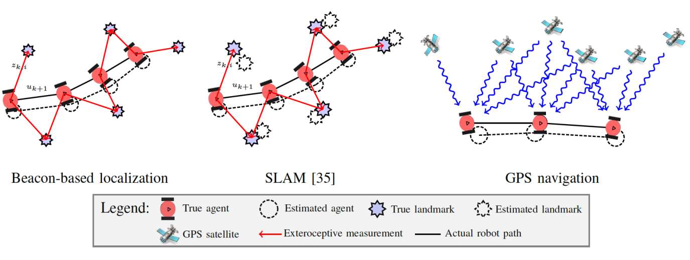
Figure 1: Schematic representation of common probabilistic localization techniques for mobile platforms: In beacon-based localization, the map of the area is known and there are pre-installed beacons or landmarks with known locations and identities. By taking relative measurements with respect to these landmarks, the mobile agents can improve their localization accuracy. For operations where a priori knowledge about the environment is not available, but nevertheless, the environment contains fixed and distinguishable features that agents can measure, SLAM is normally used to localize the mobile agents. SLAM is a process by which a mobile agent can build a map of an environment and at the same time use this map to deduce its location. On the other hand, GPS navigation provides location and time information in all weather conditions, anywhere on or near the earth but it requires an clear line of sight to at least four GPS satellites.

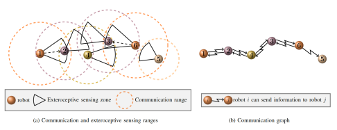
Figure 2: This figure depicts a multi-hop communication scenario for the multi-robot team. Plot (a) shows the communication and measurement ranges. Here, robots $1$ and $6$ make relative measurements, respectively, of robots $2$ and $3$. Plot (b) shows the communication graph generated using the communication ranges given in plot (a). Here the robot at the head of an arrow can send information to the robot at the tip of the arrow. As this graph shows, each of robots $1$ and $6$ can pass communication message to the entire team via a multi-hop strategy.

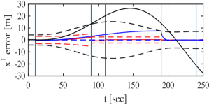
(a)

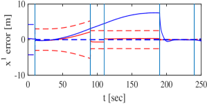
(b)

$\quad\quad\quad~{}~{}~{}~{}\quad\quad\quad\quad\quad 1\!\to\!2\quad\quad~{}\,3\!\!\to\!\!1~{}\,1\!\!\to\!\!3,3\!\!\to\!\!2,2\!\!\to\!\!1\quad\quad 1\!\to\!1$ $~{}~{}\quad\quad\quad~{}~{}~{}~{}\quad\quad\quad\quad\quad 1\!\to\!2\quad\quad~{}\,3\!\!\to\!\!1~{}\,1\!\!\to\!\!3,3\!\!\to\!\!2,2\!\!\to\!\!1\quad\quad 1\!\to\!1$

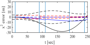
(c)

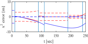
(d)

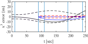
(e)

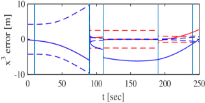
(f)

Figure 3: Estimation error (solid line) and $3\sigma$ error bounds (dashed lines) in the $x-$coordinate variable for 3 robots moving on a flat terrain when they (a) only propagate their equations of motion using self-motion measurements (black plots), (b) employ cooperative localization ignoring past correlations between the estimations of the robots (blue plots), (c) employ cooperative localization with accurate account of past correlations (red plots). The figures on the right column are the same figures as on the left where the localization case (a) is removed for clearer demonstration of cases (b) and (c). Here, $a\to b$ over the time interval marked by two vertical blue lines indicates that robot $a$ has taken a relative measurement with respect to robot $b$ at that time interval. The symbol $a\to a$ means that robot $a$ obtains an absolute measurement.

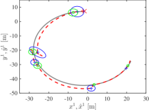
(a) Robot 1

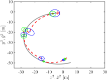
(b) Robot 2

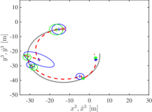
(c) Robot3

Figure 4: Trajectories of the robots for the simulation study of Fig. 3. Here, the gray curve is the ground truth. The red curve is the estimation of the trajectory by implementing a EKF CL. The blue (resp. green) ellipses show the 95% uncertainty regions for the estimations at 2 seconds before (resp. after) any change in the measurement scenario (see Fig. 3)

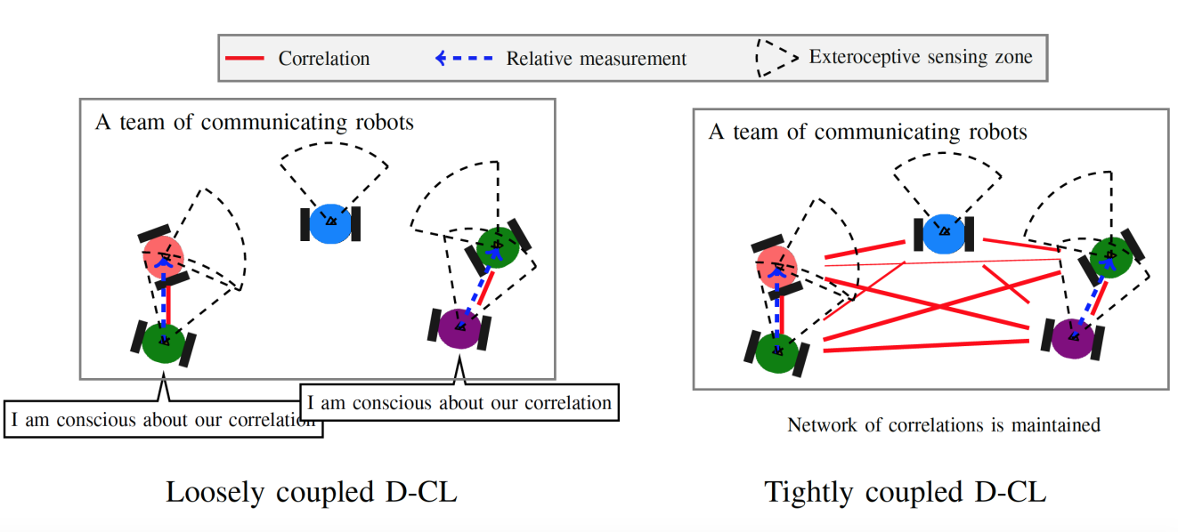
Figure 5: Schematic representation of the D-CL classification based on how the past correlations are accounted for.

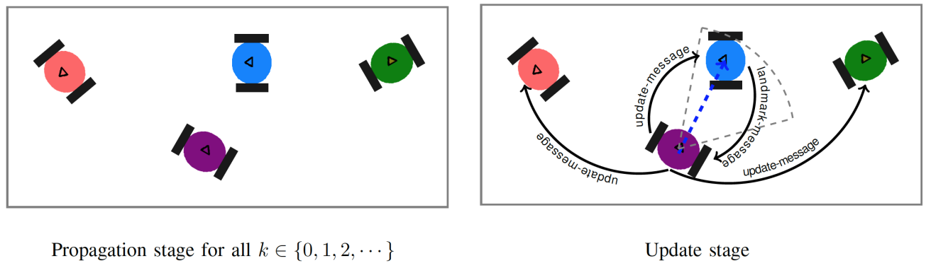
Figure 6: The in-network information flow of the Interim Master D-CL algorithm. In the Interim Master D-CL algorithm, communication is only needed in the update stage when the team members use a robot-to-robot relative measurement feedback to correct their pose estimation. Here, we assume that all the team members are in the communication range of the interim master robot.

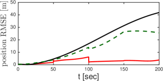
(a) Robot 1

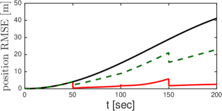
(b) Robot 2

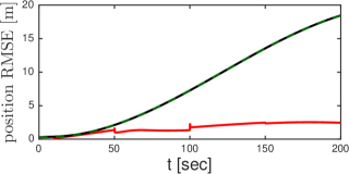
(c) Robot3

Figure 7: A comparison study between the positioning accuracy of 3 robots employing the Interim Master D-CL algorithm (red plots), with that from the EKF Covariance-Intersection based CL algorithm of [25] (dashed green plot). The curves in black show the positioning accuracy when the robots do not use any CL. As expected, the Interim Master D-CL algorithm by keeping an accurate account of the cross-covariances produces more accurate localization results than the algorithm of [25] . However, this higher accuracy comes with higher communication and processing cost per robot. Notice here that using algorithm of [25] robot $3$ does not get to update its estimation equations.

A performance analysis of an EKF CL for a team of homogeneous robots moving on a flat terrain, with the same level of uncertainty in their proprioceptive measurements and exteroceptive sensors that measure relative pose, is provided in [S1] and  [S2]. Interestingly, [S1] shows that the rate of uncertainty growth decreases as the size of the robot team increases, but is subject to the law of diminishing returns. Moreover, [S2] shows that the upper bound on the rate of uncertainty growth is independent of the accuracy or the frequency of the robot-to-robot measurements. The consistency of EKF CL from the perspective of observability is studies in [S3]. Huang et al. in [S3] analytically show that the error-state system model employed in the standard EKF CL always has an observable subspace of higher dimension than that of the actual nonlinear CL system. This results in an unjustified reduction of the EKF covariance estimates in directions of the state space where no information is available, and thus leads to inconsistency. To address this problem, Huang et al. in [S3] adopt an observability-based methodology for designing consistent estimators in which the linearization points are selected to ensure a linearized system model with an observable subspace of the correct dimension. More results on observability analysis of CL can be found in [22, S4, S5]. The use of an observability analysis to explicitly design an active local path planning algorithm for unmanned aerial vehicles implementing a bearing-only CL is discussed in [S6]. The necessity for an initialization procedure for CL is discussed in [S7]. There it is shown that, because of system nonlinearities and the periodicity of the orientation, initialization errors can lead to erroneous results in covariance-based filters. An initialization procedure for the state estimation in a CL scenario based on ranging and dead reckoning is studied in [S8].

Authors Information

Solmaz S. Kia is an Assistant Professor in the Department of Mechanical and Aerospace Engineering, University of California, Irvine (UCI). She obtained her Ph.D. degree in Mechanical and Aerospace Engineering from UCI, in 2009, and her M.Sc. and B.Sc. in Aerospace Engineering from the Sharif University of Technology, Iran, in 2004 and 2001, respectively. She was a senior research engineer at SySense Inc., El Segundo, CA from Jun. 2009-Sep. 2010. She held postdoctoral positions in the Department of Mechanical and Aerospace Engineering at the UC San Diego and UCI. Dr. Kia’s main research interests, in a broad sense, include distributed optimization/coordination/estimation, nonlinear control theory and probabilistic robotics.

Stephen Rounds is a Research Engineer with NavCom Technology, a John Deere company. He is responsible for identifying and supporting new navigation technologies for the company and developing and maintaining the intellectual property portfolio of the company. Prior to working with John Deere, Mr. Rounds worked with multiple defense contractors, with a special emphasis on GPS-denied navigation, GPS anti-jamming protection, and other sensor fusion applications. Mr. Rounds holds a B.S. degree in physics from Stevens Institute of Technology in Hoboken, N.J., and an M.S. degree in nuclear physics from Yale University. He is the Chairman of the Southern California section of the Institute Of Navigation, holds multiple patents in the navigation field, and has numerous publications in various aerospace and navigation forums.

Sonia Martínez is a Professor with the department of Mechanical and Aerospace Engineering at the University of California, San Diego. Dr. Martinez received her Ph.D. degree in Engineering Mathematics from the Universidad Carlos III de Madrid, Spain, in May 2002. Following a year as a Visiting Assistant Professor of Applied Mathematics at the Technical University of Catalonia, Spain, she obtained a Postdoctoral Fulbright Fellowship and held appointments at the Coordinated Science Laboratory of the University of Illinois, Urbana-Champaign during 2004, and at the Center for Control, Dynamical systems and Computation (CCDC) of the University of California, Santa Barbara during 2005. In a broad sense, Dr. Martínez’s main research interests include the control of networked systems, multi-agent systems, nonlinear control theory, and robotics. For her work on the control of underactuated mechanical systems she received the Best Student Paper award at the 2002 IEEE Conference on Decision and Control. She was the recipient of a NSF CAREER Award in 2007. For the paper “Motion coordination with Distributed Information,” co-authored with Jorge Cortés and Francesco Bullo, she received the 2008 Control Systems Magazine Outstanding Paper Award. She has served on the editorial boards of the European Journal of Control (2011-2013), and currently serves on the editorial board of the Journal of Geometric Mechanics and IEEE Transactions on Control of Networked Systems.

References

- [1] J. Leonard and H. F. Durrant-Whyte. Mobile robot localization by tracking geometric beacons. IEEE Transactions on Robotics and Automation, 7(3):376–382, June 1991.
- [2] G. Dissanayake, P. Newman, H. F. Durrant-Whyte, , S. Clark, and M. Csorba. A solution to the simultaneous localization and map building (SLAM) problem. IEEE Transactions on Robotics and Automation, 17(3):229–241, 2001.
- [3] S. Cooper and H. Durrant-Whyte. A Kalman filter model for GPS navigation of land vehicles. In IEEE/RSJ Int. Conf. on Intelligent Robots & Systems, pages 157–163, Munich, Germany, 1994.
- [4] J. S. Jennings, G. Whelan, and W. F. Evans. Cooperative search and rescue with a team of mobile robots. In Int. Conf. on Advanced Robotics, pages 193–200, 1997.
- [5] A. Davids. Urban search and rescue robots: from tragedy to technology. IEEE Intelligent Systems, 17(2):81–83, March-April 2002.
- [6] N. Bulusu, J. Heidemann, and D. Estrin. GPS-less low-cost outdoor localization for very small devices. IEEE Personal Communications, 7(5):28–34, 2000.
- [7] M. Trincavelli, M. Reggente, S. Coradeschi, A. Loutfi, H. Ishida, and A. J. Lilienthal. Towards environmental monitoring with mobile robots. In IEEE/RSJ Int. Conf. on Intelligent Robots & Systems, pages 2210–2215, 2008.
- [8] A. Bahr, M. R. Walter, and J. J. Leonard. Consistent cooperative localization. In IEEE Int. Conf. on Robotics and Automation, pages 8908–8913, Kobe, Japan, May 2009.
- [9] H. Mokhtarzadeh and D Gebre-Egziabher. Cooperative inertial navigation. Navigation: Journal of the Institute of Navigation, 61(2):77–94, 2014.
- [10] R. Kurazume, S. Nagata, and S. Hirose. Cooperative positioning with multiple robots. In IEEE Int. Conf. on Robotics and Automation, pages 1250–1257, San Diego, CA, May 8–13 1994.
- [11] I. Rekleitis, G. Dudek, and E. Milios. Multi-robot collaboration for robust exploration. In IEEE Int. Conf. on Robotics and Automation, pages 3164–3169, 2000.
- [12] S. I. Roumeliotis. Robust mobile robot localization: from single-robot uncertainties to multi-robot interdependencies. PhD thesis, University of Southern California, 2000.
- [13] A. Howard, M. Matark, and G. Sukhatme. Localization for mobile robot teams using maximum likelihood estimation. In IEEE/RSJ Int. Conf. on Intelligent Robots & Systems, volume 1, pages 434–439, 2002.
- [14] E. D. Nerurkar, S. I. Roumeliotis, and A. Martinelli. Distributed maximum a posteriori estimation for multi-robot cooperative localization. In IEEE Int. Conf. on Robotics and Automation, pages 1402–1409, Kobe, Japan, May 2009.
- [15] D. Fox, W. Burgard, H. Kruppa, and S. Thrun. A probabilistic approach to collaborative multi-robot localization. Autonomous Robots, 8(3):325–344, 2000.
- [16] A. Howard, M. J. Mataric, and G. S. Sukhatm. Putting the ‘I’ in ‘team’: An ego-centric approach to cooperative localization. In IEEE Int. Conf. on Robotics and Automation, volume 1, pages 868– 874, 2003.
- [17] A. Prorok and A. Martinoli. A reciprocal sampling algorithm for lightweight distributed multi-robot localization. In IEEE/RSJ Int. Conf. on Intelligent Robots & Systems, pages 3241–3247, 2011.
- [18] A. T. Ihler, J. W. Fisher, R. L. Moses, and A. S. Willsky. Nonparametric belief propagation for self-localization of sensor networks. IEEE Journal of Selected Areas in Communications, 23(4):809–819, 2005.
- [19] J. Nilsson, D. Zachariah, I. Skog, and P. Händel. Cooperative localization by dual foot-mounted inertial sensors and inter-agent ranging. EURASIP Journal on Advances in Signal Processing, 2013(164), 2013.
- [20] A. Howard, M. J. Matarić, and G. S. Sukhatme. Mobile sensor network deployment using potential fields: A distributed scalable solution to the area coverage problem. In Int. Conference on Distributed Autonomous Robotic Systems, pages 299–308, Fukuoka, Japan, June 2002.
- [21] S. S. Kia, S. Rounds, and S. Martínez. A centralized-equivalent decentralized implementation of extended Kalman filters for cooperative localization. In IEEE/RSJ Int. Conf. on Intelligent Robots & Systems, pages 3761–3765, Chicago, IL, September 2014.
- [22] S. I. Roumeliotis and G. A. Bekey. Distributed multirobot localization. IEEE Transactions on Robotics and Automation, 18(5):781–795, 2002.
- [23] C. T. Leondes, editor. Advances in Control Systems Theory and Application, volume 3. Academic Press, New York, 1966.
- [24] Y. Bar-Shalom, P. K. Willett, and X. Tian. Tracking and Data Fusion, a Handbook of Algorithms. YBS Publishing, Storts, CT, USA, 2011.
- [25] L. C. Carrillo-Arce, E. D. Nerurkar, J. L. Gordillo, and S. I. Roumeliotis. Decentralized multi-robot cooperative localization using covariance intersection. In IEEE/RSJ Int. Conf. on Intelligent Robots & Systems, pages 1412–1417, Tokyo, Japan, 2013.
- [26] P. O. Arambel, C. Rago, and R. K. Mehra. Covariance intersection algorithm for distributed spacecraft state estimation. In American Control Conference, pages 4398–4403, Arlington, VA, 2001.
- [27] H. Li and F. Nashashibi. Cooperative multi-vehicle localization using split covariance intersection filter. IEEE Intelligent Transportation Systems Magazine, 5(2):33–44, 2013.
- [28] D. Marinescu, N. O’Hara, and V. Cahill. Data incest in cooperative localisation with the common past-invariant ensemble kalman filter. pages 68–76, Istanbul, Turkey, 2013.
- [29] S. J. Julier and J. K. Uhlmann. A non-divergent estimation algorithm in the presence of unknown correlations. In American Control Conference, pages 2369–2373, Albuquerque, NM, 1997.
- [30] S. J. Julier and J. K. Uhlmann. Simultaneous localisation and map building using split covariance intersection. In IEEE/RSJ Int. Conf. on Intelligent Robots & Systems, pages 1257–1262, Maui, HI, 2001.
- [31] N. Trawny, S. I. Roumeliotis, and G. B. Giannakis. Cooperative multi-robot localization under communication constraints. In IEEE Int. Conf. on Robotics and Automation, pages 4394–4400, Kobe, Japan, May 2009.
- [32] K. Y. K. Leung, T. D. Barfoot, and H. H. T. Liu. Decentralized localization of sparsely-communicating robot networks: A centralized-equivalent approach. IEEE Transactions on Robotics, 26(1):62–77, 2010.
- [33] L. Paull, M. Seto, and J. J. Leonard. Decentralized cooperative trajectory estimation for autonomous underwater vehicles. In IEEE/RSJ Int. Conf. on Intelligent Robots & Systems, pages 184–191, 2014.
- [34] S. S. Kia, S. Rounds, and S. Mart/’/inez. Cooperative Localization under message dropouts via a partially decentralized EKF scheme. In IEEE Int. Conf. on Robotics and Automation, Seattle, WA, May 2015.
- [35] H. Durrant-Whyte and T. Bailey. Simultaneous localization and mapping: Part i. 13(2):99–110, 2006.

References

- [S1] S. I. Roumeliotis and A. I. Mourikis. Propagation of uncertainty in cooperative multirobot localization: Analysis and experimental results. Autonomous Robots, 17(1):1573–7527, 2004.
- [S2] A. I. Mourikis and S. I. Roumeliotis. Performance analysis of multirobot cooperative localization. IEEE Transactions on Robotics, 22(4):666–681, 2006.
- [S3] G. Huang, N. Trawny, A. I. Mourikis, and S. I. Roumeliotis. Observability-based consistent EKF estimators for multi-robot cooperative localization. Autonomous Robots, 30(1):37–58, 2011.
- [S4] A. Martinelli and R. Siegwart. Observability analysis for mobile robot localization. In IEEE/RSJ Int. Conf. on Intelligent Robots & Systems, pages 1471–1476, 2005.
- [S5] R. Sharma, R. W. Beard, C. N. Taylor, and S. Quebe. Graph-based observability analysis of bearing-only cooperative localization. IEEE Transactions on Robotics, 28(2):522–529, 2012.
- [S6] R. Sharma. Bearing-Only Cooperative-Localization and Path-Planning of Ground and Aerial Robots. PhD thesis, Brigham Young University, 2011.
- [S7] N. Trawny. Cooperative localization: On motion-induced initialization and joint state estimation under communication constraint. PhD thesis, University of Minnesota, 2010.
- [S8] J. Nilsson and P. Händel. Recursive bayesian initialization of localization based on ranging and dead reckoning. In IEEE/RSJ Int. Conf. on Intelligent Robots & Systems, pages 1399–1404, 2013.