The effect of craters on the lunar neutron flux

Abstract

The variation of remotely sensed neutron count rates is measured as a function of cratercentric distance using data from the Lunar Prospector Neutron Spectrometer. The count rate, stacked over many craters, peaks over the crater centre, has a minimum near the crater rim and at larger distances it increases to a mean value that is up to $1\%$ lower than the mean count rate observed over the crater. A simple model is presented, based upon an analytical topographical profile for the stacked craters fitted to data from the Lunar Orbiter Laser Altimeter (LOLA). The effect of topography coupled with neutron beaming from the surface largely reproduces the observed count rate profiles. However, a model that better fits the observations can be found by including the additional freedom to increase the neutron emissivity of the crater area by $\sim 0.35\%$ relative to the unperturbed surface. It is unclear what might give rise to this effect, but it may relate to additional surface roughness in the vicinities of craters. The amplitude of the crater-related signal in the neutron count rate is small, but not too small to demand consideration when inferring water-equivalent hydrogen (WEH) weight percentages in polar permanently shaded regions (PSRs). If the small crater-wide count rate excess is concentrated into a much smaller PSR, then it can lead to a large bias in the inferred WEH weight percentage. For instance, it may increase the inferred WEH for Cabeus crater at the Moon’s South Pole from $\sim 1\%$ to $\sim 4\%$.

Eke et al. Lunar craters and neutron fluxes

1 Introduction

Cosmic ray interactions with planetary surfaces lead to nuclear fragments being released in the regolith. The study of neutrons that avoid nuclear recapture and subsequently escape through the surface provides a route to determining the abundance of various nuclei near the surface of those bodies (Lingenfelter et al., 1961; Metzger and Drake, 1990; Feldman et al., 1991). Of particular interest is the epithermal neutron flux (energies in the range $0.3$ eV$<E<0.5$ MeV), because of its sensitive dependence on the hydrogen abundance in the top $\sim 70$ cm of regolith (Feldman et al., 2000). The first experiment to search for lunar hydrogen in this way was the Lunar Prospector Neutron Spectrometer (LPNS, Feldman et al., 2004). Feldman et al. (1998) found that there were polar dips in the epithermal neutron count rate, implying the existence of polar near-surface hydrogen. Furthermore, the lack of a corresponding feature in the fast neutrons with energies exceeding $0.5$ MeV (Feldman et al., 1998) or the thermal neutrons with $E<0.3$ eV (Lawrence et al., 2006) suggested that any hydrogen-rich layer of material should be buried beneath $5-10$ cm of hydrogen-poor material.

The omni-directional LPNS, when orbiting at $30$ km, had a spatial footprint with a full-width half-maximum (FWHM) on the lunar surface of $45$ km (Maurice et al., 2004). In order to suppress statistical noise, Feldman et al. (1998) and Feldman et al. (2001) binned the data into $\sim 60$ km $\times 60$ km pixels. This is large relative to the sizes of most permanently shaded regions. However, Eke et al. (2009) showed, by stacking data and using a pixon-based image reconstruction technique to improve the spatial resolution while suppressing the noise, that these count rate dips could, in a statistical sense, be associated with the permanently shaded regions. This result was confirmed by Teodoro et al. (2010) using a more accurate set of permanently shaded regions defined by the SELENE laser altimeter (Noda et al., 2008). The count rate dip inferred for Cabeus crater corresponded to a $(1\pm 0.3)~{}{\rm wt}\%$ water equivalent hydrogen (WEH) according to the regolith composition model of Lawrence et al. (2006), which has a semi-infinite layer of ferroan anorthosite (FAN)-type soil with varying amounts of H₂O.

Another experiment, the Lunar Exploration Neutron Detector (LEND), contained sensors called the Collimated Sensor for EpiThermal Neutrons (CSETN) and the Sensor for EpiThermal Neutrons (SETN, Mitrofanov et al., 2010). These mapped the Moon from the Lunar Reconnaissance Orbiter at an altitude of $50$  km, $\sim 20$ km above the orbit of Lunar Prospector. Thus, one should not expect the SETN instrument to provide competitive results relative to the LPNS. Furthermore, comprehensive analyses of the data returned from the CSETN have demonstrated that the collimator did not perform well enough to fulfil its mission objectives (Lawrence et al., 2011a; Miller et al., 2012), with the vast majority of lunar neutrons being uncollimated (Eke et al., 2012) and an effective FWHM much larger than that of the omni-directional LPNS (Teodoro et al., 2014). In view of the difficulties associated with the interpretation of this data set, these data will be considered only briefly in this paper.

The Lunar Crater Observation and Sensing Satellite (LCROSS) impacted into Cabeus crater in 2009 and the resulting ejecta plume was analysed to give a value of $(5.6\pm 2.9)~{}{\rm wt}\%$ WEH (Colaprete et al., 2010). While statistically consistent with the LPNS result, the most probable value is over five times the LPNS-inferred value. The reanalysis of the LCROSS data by Strycker et al. (2013), which gave $(6.3\pm 1.6)~{}{\rm wt}\%$ WEH, is inconsistent with the LPNS result. These comparisons would be affected if the hydrogen detected by the LPNS was not uniformly spread across the surface within the large resolution element, which is approximately 1000 times as long as the crater produced by the LCROSS impact (Schultz et al., 2010). The LPNS and LCROSS results sample somewhat different depths into the regolith. Thus, any variation in hydrogen content with depth could also lead to a difference between the hydrogen abundances inferred from the two separate methods. One assumption that is implicit in the studies of craters using the LPNS data is that neutron count rates are not explicitly affected by the surface topography. A new model will be presented in this paper to quantify the topographical effect from craters on the neutron count rate.

The Chandrayaan-1 M³ results interpreted as implying a particular excess of water or hydroxyl molecules in Goldschmidt crater (Pieters et al., 2009) prompted Lawrence et al. (2011b) to re-examine LPNS data in this region in the context of a two-layer regolith model, with the surface layer being hydrogen-rich. This contrasted with previous Monte Carlo modelling of the lunar regolith, where the hydrogen had been buried under a dry layer of regolith (Lawrence et al., 2006). After removal of the trends caused by bulk composition, the thermal and epithermal data in the vicinity of Goldschmidt crater were compared with the models to investigate the sensitivity of neutron measurements to the depth distribution of hydrogen. Lawrence et al. (2011b) concluded that it was necessary to understand more about systematic variations at the $1-3\%$ level before definitive conclusions could be reached. If crater topography does provide small systematic variations in neutron count rates then it needs to be understood in order to progress.

When studying the LPNS count rate, Feldman et al. (2001) found that ‘local maxima overlay the floors of large, flat-bottomed craters’. They did not speculate as to what this implied, but the possibility of a topographical effect on the measured neutron count rate is one that could create a systematic bias in the values of WEH inferred above permanently shaded polar craters. To date there has been no systematic, quantitative study of the imprint of topographical features on the detected orbital neutron count rate. It is important to quantify the impact of topography on the emitted lunar neutron flux because many of the results from the LPNS involve small changes in count rates measured over craters.

Section 2 contains a description of the neutron and topography data being used. Fits to the crater average topography are given in Section 3. The variation of neutron count rate as a function of distance to the crater centre is shown in Section 4, for a variety of different subsets of craters. In Section 5, a simple model is presented for how the neutron count rate changes as a function of detector distance from the crater centre. This model is confronted with the data, and the implications for our understanding of the regolith are investigated. Section 6 discusses the implications of this work for quantitative estimates of cold-trapped hydrogen, and conclusions are drawn in Section 7.

2 Data

Maps of the lunar neutron count rate, a set of predetermined lunar craters and a digital elevation map are necessary to calculate the neutron count rate profiles near craters. The data sets to be used here, which are all available from the Geosciences Node of NASA’s Planetary Data System (PDS), are described in this section.

2.1 Lunar Prospector neutron data

The Lunar Prospector spacecraft spent one year at $100$ km altitude, then seven months at $40-30$ km. PDS time series data from the thermal, epithermal and fast neutron detectors, processed as described by Maurice et al. (2004), are used in this study, with the focus mainly on the low-altitude subset. Some results from the high-altitude period will also be shown for comparison, but the default choice is to consider only data for which Lunar Prospector was at an altitude less than $45$ km. Using different energy neutrons is desirable because of their differing responses to changes in regolith composition. Also, the thermal neutrons probe further into the regolith than the epithermals, whereas the fast neutrons typically sample nearer to the surface than the epithermals.

2.2 Lunar Exploration Neutron Detector data

Data from the first 15 months of the mapping orbits are used for both the LEND SETN and CSETN detectors, to compare with the results from the LPNS. For the CSETN measurements the background due to cosmic rays striking the spacecraft itself is removed statistically following the procedure described by Eke et al. (2012). The remaining count rate is comprised of two distinct lunar components, where the detected neutrons originate either from within or outside the collimator’s geometrical field-of-view. One cannot determine from which component individual neutrons originate.

2.3 Crater list and topographical data

The list of craters produced by Head et al. (2010) from the Lunar Orbiter Laser Altimeter (LOLA) topographical data is used. This consists of 5185 craters with radii of at least $10$ km, distributed over the entire lunar surface. In this study, various different selections of craters are made, based on the radii, $r_{c}$, and the central locations given in this list. The variable $r$ will be used here to represent arclengths along an unperturbed spherical surface, whereas the variable $x$ represents the distance from the symmetry axis ($z$) of a crater. Thus, the measured crater diameters are really $2x_{\rm c}$ in this nomenclature. $x$ and $r$ are related via

$$x=r_{\rm m}\sin\left(\frac{r}{r_{\rm m}}\right),$$ (1)

where $r_{\rm m}=1737.4$ km is the lunar radius. This equation implies that $x_{\rm c}$ will be within $0.1\%$ of $r_{c}$ for crater radii less than $100$ km, so the variables $x_{\rm c}$ and $r_{c}$ will be assumed to be equal for the rest of this study. The angle subtended at the lunar centre by the crater radius is

$$\theta_{c}=\sin^{-1}\left(\frac{x_{\rm c}}{r_{\rm m}}\right).$$ (2)

The global topographic map from LOLA (Smith et al., 2010) with $(1/64)^{\circ}$ resolution is used to measure the crater topographical profiles. This corresponds to $\sim 0.5$ km resolution at the equator, which is more than sufficient for the approximate modelling of crater topography as a function of crater radius that is necessary for the neutron count rate model presented in Section 5.

The epithermal neutron count rate measured by the omnidirectional LP detector changes by approximately $10\%$ across the whole Moon. This variation is dominated by known changes in regolith composition. Any systematic topographical effects are expected to be at the level of $\sim 1\%$, as noted by Feldman et al. (2001). This anticipated variation is sufficiently small that it is necessary to stack together craters of similar size in order to reduce the statistical uncertainties. In addition, the stacking averages away azimuthal anisotropy that exists in the crater sample, making radial profiles an appropriate way to represent the results. To produce a more homogeneous set of craters to stack together, both in terms of topography and composition, only craters in ‘highland’ regions will be considered in this study. This means only craters on the far side of the Moon and with latitudes greater than $-20^{\circ}$ will be included in the stacking procedure. These cuts leave just 2216 craters. This choice is important for some of the results presented later involving thermal and fast neutrons, which are both more sensitive than epithermal neutron fluxes to iron and titanium abundances.

3 Crater topography

The model for the topographical effect on the neutron count rate described in Section 5 needs to assume a particular crater profile. This section first describes the functional form of the assumed crater profile, then measures it using the LOLA digital elevation map by stacking radial profiles for craters in the chosen range of sizes.

3.1 Model crater profile

Table 1: Least-squares parameter values for the crater topography model fitted to the stacked LOLA data as a function of crater radius.a

Crater radius, $r_{c}/$km	Number of craters	Depth, $d$/km	Infill radius, $x_{\rm i}/x_{\rm c}$	Edge of outer slope, $x_{\rm e}/x_{\rm c}$	Uplift, $u$/km
$10-20$	1264	$2.00$	$0.30$	$2.1$	$0.45$
$20-30$	482	$2.50$	$0.42$	$2.1$	$0.60$
$30-40$	219	$2.75$	$0.48$	$2.0$	$0.70$
$40-50$	115	$3.25$	$0.56$	$2.2$	$0.85$
$50-60$	47	$3.70$	$0.66$	$2.1$	$1.15$
$60-80$	42	$3.40$	$0.70$	$1.8$	$1.00$
$40-50$ deep	57	$4.05$	$0.48$	$2.2$	$1.15$
$40-50$ shallow	58	$3.05$	$0.69$	$2.1$	$0.65$

aThe depth, fractional infill radius, fractional edge of outer slope and uplift are found on grids with resolution $0.05$ km, $0.01$, $0.01$, and $0.05$ km respectively, which are larger than the statistical uncertainties on these parameters. The midpoint of the crater radius range is used to calculate the parameters for each stacked profile.

Figure 1: Model crater profile (bold line) that is fitted to the LOLA topographical data for the selected craters. The model takes into account a flat infill region at radii less than $x_{\rm i}$, a spherical cap depression out to $x_{\rm c}$ and an outer slope, uplifted at the crater rim by an amount $u$, that returns to the unperturbed surface at $x_{\rm e}$. The centre of the Moon is used as the origin of the coordinate system.

Rather than having a general topography, the model craters in Section 5 are considered to have azimuthally symmetric profiles of a kind shown in Figure 1. These consist of a spherical cap depression of depth $d$ measured down from the $x-y$ plane containing the crater rim, with a central, flat ($dz/dx=0$) infill region extending out to a radius $x_{\rm i}$, and with a maximum depth, at $x=0$ of $d_{\rm i}$, where the i subscript refers to the infill region. The radius of curvature for the spherical cap part of the crater is then

$$r_{\rm curv}=\frac{x_{\rm c}^{2}+d^{2}}{2d},$$ (3)

and the maximum infill depth, measured from the base of the spherical cap to the infill surface, is given by

$$d_{i}=r_{\rm curv}-\sqrt{r_{\rm curv}^{2}-x_{\rm i}^{2}}.$$ (4)

This crater is uplifted parallel to the crater axis (the $z$ direction) by a distance $u$, with an outer slope of constant gradient, $dz/dx\equiv g$, back to the unperturbed surface at a perpendicular distance of $x_{\rm e}$ from the symmetry axis of the crater. Defining

$$\theta_{e}=\sin^{-1}\left(\frac{x_{\rm e}}{r_{\rm m}}\right),$$ (5)

the gradient of the outer slope is given by

$$g=\frac{r_{\rm m}\cos\theta_{e}-(r_{\rm m}\cos\theta_{c}+u)}{x_{\rm e}-x_{\rm c}}.$$ (6)

The height of the crater relative to an unperturbed surface can be found using

$$h(x)=\sqrt{x^{2}+z(x)^{2}}-r_{\rm m},$$ (7)

where $z$ is defined as zero at the lunar centre. For $x\geq x_{\rm e}$, $h=0$ for the model crater. At $x=0$,

$$z(x=0)\equiv z_{0}=r_{\rm m}\cos\theta_{c}-d+u+d_{i}.$$ (8)

At radii where the presence of the crater perturbs the surface, the height can be inferred using the following expression for $z$:

$$z(x)=\left\{\begin{array}[]{ll}z_{0}&\mbox{if $x\leq x_{\rm i}$~{};}\\ z_{0}-d_{i}+r_{\rm curv}-\sqrt{r_{\rm curv}^{2}-x^{2}}&\mbox{if $x_{\rm i}\leq x\leq x_{\rm c}$~{};}\\ z_{c}+g(x-x_{\rm c})&\mbox{if $x_{\rm c}\leq x\leq x_{\rm e}$~{}.}\end{array}\right.$$ (9)

$z_{c}$ represents $z(x_{\rm c})\equiv z_{0}-d_{i}+r_{\rm curv}-\sqrt{r_{\rm curv}^{2}-x_{\rm c}^{2}}$.

A least-squares minimisation was performed to find the best-fitting sets of the parameters $[d,x_{\rm i},u,x_{\rm e}]$ for the subsets of craters of different radius. For all subsets of craters with radii of at least $20$ km, the region at $x<0.2x_{\rm c}$ was excluded from the fit, because a central peak, not included in the model, often exists. The midpoint of the crater radius bin was chosen for the $x_{\rm c}$ of the model to be fitted to the stacked profile.

3.2 Crater topography fits

For each crater, digital elevation map measurements within $3r_{c}$ were used to construct the relative height profile as a function of $r/r_{c}$, where $r$ represents the arc length from the crater centre to the spacecraft nadir. The zero of height for each crater is defined as the mean height in the range $2.5<r/r_{c}<3$. Each measurement provides an estimate of the relative height at its $r/r_{c}$. The statistical uncertainty on the estimated mean height is just the square root of the ratio of the variance of the individual measurements within a given bin in $r/r_{c}$ to the number of observations in that bin. The craters were stacked by crater radius, because the typical crater shape varies systematically with crater radius.

The crater set with $40<r_{c}/$km$<50$ was further subdivided by depth to see how this affected the neutron count rate profiles. To split the crater subset by crater depth, in order to investigate the effect on the neutron profile, the depth of each crater is defined as the difference between the average heights in the radial ranges $(0.95-1)r_{c}$ and $(0.2-0.3)r_{c}$. The central region is once again avoided to reduce any systematic effect due to central peaks. While this statistic might, in some instances, reflect subcraters rather than the larger scale topography, it at least serves as a simple way to separate deep and shallow craters with the same radius.

Figure 2 shows the azimuthally averaged mean radial topographical profiles for craters of different sizes, as measured using craters from the Head et al. (2010) list and LOLA topographical data. Statistical errors on the mean profiles are smaller than the symbol sizes. It is apparent that for the larger craters there are central peaks that are not included in the model profile, as described in the previous section.

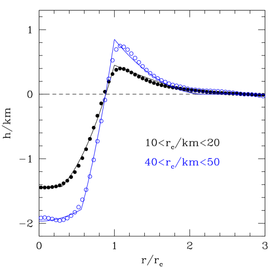
Figure 2: Mean radial LOLA topographical profiles for craters with radii in the ranges $10-20$ km (black filled circles) and $40-50$ km (blue open circles). Statistical errors on the mean profiles are smaller than the symbol sizes. Solid lines show the least-squares model fits to the data sets as detailed in equations (1-9).

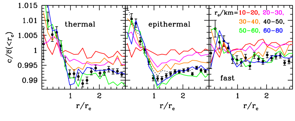
Figure 3: Stacked, normalised radial LP neutron mean count rate profiles for different radius craters. Thermal, epithermal and fast neutron results are shown in the left, centre and right panels respectively. The different colours correspond to craters in the radius ranges $10-20$ km (red), $20-30$ km (magenta), $30-40$ km (orange), $40-50$ km (black points), $50-60$ km (green) and $60-80$ km (blue). A black dotted line represents the epithermal neutron profile for $40-50$ km craters when the time series is sampled in $32$ s observations, like the fast neutron data set, rather than $8$ s like the thermal and epithermal time series.

The best-fitting models are also shown in Figure 2, from which it can be seen that the model becomes increasingly inappropriate for larger craters. A flat, $dz/dx=0$ central region does not translate to a constant height relative to the unperturbed spherical surface, which would provide a better fit to the $r_{c}>70$ km craters. Also, the constant $dz/dx$ outer slope, at large distances, can lead to $h<0$ on the outer uplifted slope; a feature not present in the observations. Despite these shortcomings in the model, it does capture the main features present in the measured average topographical profiles, and the extent to which the model is inadequate is not quantitatively significant for the neutron count rate results in subsequent sections.

Table 1 lists the best-fitting model parameters for a set of different crater size ranges. These values are used in Section 5 for the model predicting the topographical effect on the neutron count rate profiles observed by the orbiting detector. The depth parameter, $d$, only represents the depth of the crater when there is no infill so, as can be seen by comparing the values in Table 1 with the data in Figure 2, the actual crater depths from rim to minimum are typically much smaller than $d$. This is particularly true for the larger craters, where the best-fitting infill region extends to a larger fraction of the crater radius.

4 Neutron count rate profiles

For each crater, time series observations within $3r_{c}$ were used to construct relative count rate profiles, where the relative count rate is defined for each crater by dividing each time series measurement by the mean count rate within $r_{c}$ of the crater centre. Each time series observation provides an estimate of the relative count rate at a given $r/r_{c}$ and these are stacked together for different crater subsets.

4.1 Radial count rate variations

The results in this subsection show how the neutron count rate varies as a function of sub-detector point distance to the crater centre. Stacked subsets of similar-sized highland craters are used, as are data for different neutron energy ranges.

Figure 3 shows the mean stacked, count rate ($c$) profiles, with observations from each contributing crater normalised by the mean count rate measured from positions over that crater, $\bar{c}(<r_{c})$. As the craters are very well sampled, had the count rates instead been normalised with respect to the count rate at $r/r_{c}\sim 3$ the stacked profiles would only change by a radius-independent, vertical shift. The radii are normalised by the relevant crater radius. Points and errors on the mean profiles are shown only for the $40<r_{c}/$km$<50$ case for clarity, but are of similar size for the other crater subsets. For both the thermal and epithermal profiles, a central $\sim 1\%$ enhancement in the neutron count rate is seen, with the count rate outside the crater being $\sim 0.7\%$ lower than the mean count rate measured over the crater. These features are about twice as pronounced as those in the corresponding fast neutron profiles, and are common to all crater samples with $r_{c}>40$ km. For smaller crater sizes, the features in the profiles decrease in amplitude. Given that the FWHM of the LP neutron detectors is approximately $45$ km at an altitude of $30$ km, one should expect that any features on smaller scales will be washed out. Also, if all craters have their radii either overestimated or underestimated by $5\%$ then the changes in the neutron count rate profiles are lower than $0.1\%$, so the results are robust to this level of systematic uncertainty in the crater radius determination.

One reason why the fast neutron profile might be less variable than those in the lower energy ranges is that the temporal sampling is lower, with $32$ s observations, rather than $8$ s. At an altitude of $30$ km, LP travelled $\sim 50$ km during $32$ s. The effect of the resultant blurring of the profile can be estimated by degrading the sampling of the epithermal neutron time series. This is illustrated for the $40<r_{c}/$km$<50$ craters by the dotted line in the central panel of Fig. 3. For craters that are at least this large, the different sampling has only a small effect. However, for smaller craters, where the distance travelled during an individual observation corresponds to a larger $r/r_{c}$, the suppression of features in the normalised count rate profile will be larger. Fig. 3 suggests that any features in the fast neutron profile for craters with $r_{c}<40$ km would be small anyway.

Lunar Prospector neutron count rates are evidently affected, at the $\sim\pm 1\%$ level, by the detector position relative to craters on the surface, provided that the detector footprint is small enough to allow it to ‘see’ the craters. At this point, it is worth briefly considering the count rate profiles produced by the LEND SETN and CSETN. The SETN is an “omni-directional” detector, albeit strapped to the side of a “collimator”, so in practice it has an energy-dependent anisotropic footprint. Given that it is viewing the surface from $\sim 50$ km altitude, the features seen by the LPNS should be stronger than those recovered by the SETN. This is evident in Figure 4, which shows the count rate profiles measured by the SETN for a range of different crater sizes. The features, while still significant, have been washed out, typically decreasing the amplitude of the central peak by a factor of a few.

Figure 5 shows the spacecraft background-corrected CSETN count rate profiles. After correction, the count rates are typically only $\sim 2$ per second, hence the large statistical uncertainties. However, unlike the SETN profiles that show similar trends with crater size to the LPNS results, the CSETN profiles show no obvious trends or significant central bumps in the count rate. This is entirely consistent with the large CSETN detector footprint inferred by Teodoro et al. (2014).

Having determined that the LPNS count rate varies systematically with distance from crater centres, the question becomes what is responsible for this? One uninteresting possibility can be immediately discounted by recalculating the count rate profiles using the raw LPNS data. The features are similarly present in the raw data, implying that the data reduction process did not create them and they do reflect something to do with the lunar surface. Compositional variation would not create almost identical features in the thermal and epithermal count rate profiles. Also, if mafic and magnesian central peaks (Cahill et al., 2009) were having an important impact on these profiles, then the thermal and fast neutron profiles should be anticorrelated, whereas they show qualitatively similar behaviour. The possibility that these profiles are the result of the geometrical configuration will be considered in the following section.

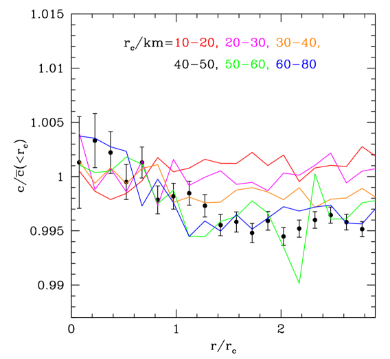
Figure 4: Stacked, normalised radial LEND SETN neutron count rate profiles for observations at altitudes less than $60$ km. The different colours correspond to different sized craters, as described in the caption for Figure 3.

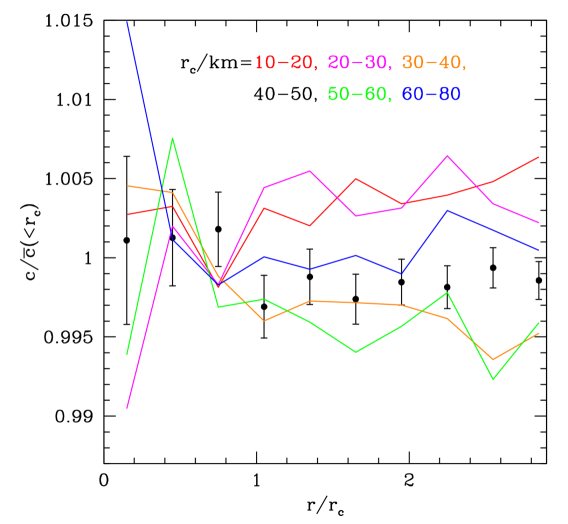
Figure 5: Stacked, normalised radial LEND CSETN neutron count rate profiles for observations at altitudes less than $60$ km. The different colours correspond to different sized craters, as described in the caption for Figure 3.

5 A Simple Geometrical Model

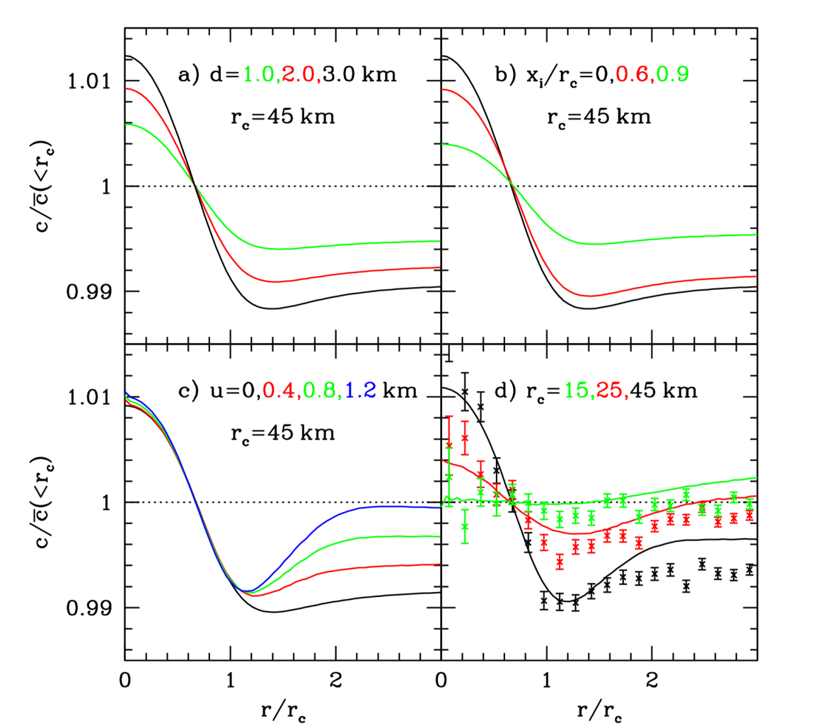
Figure 6: Variation of the model count rate profile normalised to the mean count rate over the crater. Panel (a) shows the variation with crater depth, $d$, for a $45$ km radius crater, with no infill or uplift, and the detector placed at an altitude of $30$ km. These model craters are just spherical cap depressions. Panel (b) fixes $d=3.0$ km and shows the effect of adding a flat central infill region out to a fraction $x_{\rm i}/r_{c}$ of the crater radius. Fixing $x_{\rm i}=0.6\,r_{c}$ and $x_{\rm e}=2.0\,r_{c}$, panel (c) illustrates the variation of the count rate profile with crater uplift. Finally, panel (d) shows how the model profile varies with crater radius. At each different radius, the crater shapes are defined using the appropriate parameters in Table 1. The data points show the LPNS count rate profiles for the corresponding crater stacks.

A model describing how topography affects the detected neutron flux is outlined in this section, in order to determine if this alone can explain the neutron count rate profile over craters. The predictions from this model are compared with the LPNS count rate profiles and the implications of this comparison are then discussed.

5.1 The model

The flux measured a distance $r$ away from a patch of surface area d$A$ emitting neutrons at a rate $f_{0}$ per unit area, with a detector an angle $\theta$ away from the surface normal can be written as

$${\rm d}f(r,\theta)=\frac{(2+\alpha)f_{0}}{2\pi r^{2}}\cos^{1+\alpha}\theta\,{\rm d}A,$$ (10)

where $\alpha$ represents the effective beaming of the neutrons out of the surface resulting from the increase in neutron number density with depth in the top $\sim$ mean free path in the regolith (McKinney et al., 2006). $\alpha\approx 0.5$ provides a good match to the Monte Carlo neutron transport flat surface models of Lawrence et al. (2006) for the range of neutron energies detected by the LPNS.

The model for the total flux received by the detector involves integrating equation (10) over the lunar surface that is visible from the detector, assuming that the flux from a particular piece of surface is proportional to the incident cosmic ray flux. One complication is that when the surface includes concave craters, their walls can act to block parts of the crater interior from the detector’s view. If crater uplift is included then this effect can also extend to the exterior of the crater. The model accounts for this but does not, by default, allow neutrons emitted from the crater and impinging on the crater wall to be reemitted. This assumption will be considered further in section 5.3.

In practice, the flux calculation can be more efficiently performed by partitioning the surface into different zones and using symmetries in the problem to avoid needing to do a two-dimensional numerical integration over the full visible surface. These zones are:

1. the central infilled region of the crater, $(x\leq x_{\rm i})$,
   

2. the constant radius of curvature crater walls, $(x_{\rm i}\leq x\leq x_{\rm c})$,
   

3. the outer uplifted slope, $(x_{\rm c}\leq x\leq x_{\rm e})$,
   

4. the unperturbed surface beyond the outer uplifted slope, $(x_{\rm e}\leq x)$.
   

For the more interested reader, Appendix A contains specific details of the calculations involved.

5.2 Predictions of the model

Figure 6 shows the neutron count rate profile from the model. The four panels show how the profile changes with (a) crater depth, (b) extent of the infill region, (c) amount of uplift, and (d) crater radius. In all cases the detector is placed at an altitude of $30$ km and the effective beaming of neutrons is taken to be $\alpha=0.5$. The mean altitude for the LPNS observations being considered at altitudes less than $45$ km is $\sim 31$ km.

Panels (a) and (b) show that, for a $45\,$km radius crater, as the crater becomes deeper or the infill zone smaller, the central peak in count rate over the crater increases. This happens because these changes enhance the effect of the neutron beaming seen over the crater. If the beaming of neutrons is switched off, i.e. $\alpha=0$, and neutrons are allowed to be reemitted off the crater interior, then the model has $c(r)/\bar{c}(<~{}r_{\rm c})=1$ for all $r$.

Panel (c) of Fig. 6 shows how uplifting a $45$ km crater and having a constant gradient outer slope that returns to the unperturbed surface at $x_{\rm e}=2.0\,r_{c}$ affects the neutron count rate profile. As the uplift increases, the outer uplifted slope focuses more neutrons onto the detector when it is over the crater exterior, leading to larger count rates at $r/r_{\rm c}>1$.

The variation of the model count rate profile with crater radius is shown in panel (d). Parameters for the model crater shapes are taken from the fits to the stacked LOLA topographical profiles, as listed in Table 1. For the $15$ km radius craters, the central peak in the count rate profile occurs on scales too small for the $45$ km FWHM of an omnidirectional detector at an altitude of $30$ km. Consequently, the profile looks almost flat. For larger craters, the central peak in neutron count rate becomes increasingly apparent as the instrumental FWHM corresponds to smaller $r/r_{c}$. The simple geometrical model captures much of the central bump that is present in the data for the different crater sizes. However, more apparent is the failure to reproduce the LPNS results at $r/r_{\rm c}\mathrel{\hbox{\hbox to0.0pt{\hbox{\lower 4.0pt\hbox{$\sim$}}\hss}\hbox{$>$}}}2$, where the model overpredicts the observed count rate by $\sim 0.3\%$.

The features of the comparison between model and LPNS neutron count rate profiles are common across the different crater sizes, in both the deep and shallow craters, and when the observations are split into high and low altitude subsets and the model is adjusted accordingly. In all cases, the model appears slightly to underestimate the count rate observed over the crater. Given that this provides the normalisation for all count rates, a consequence is that the model overestimates the normalised count rate at large distances from the crater.

One might wonder if the stacking process, used here to increase the statistical significance of the measured average neutron count rate profile features, might introduce systematic effects. For instance, not all craters in a particular radius range have identical topographical profiles. If the neutron count rate profile features were especially sensitive to the deepest craters, which might have only a small impact on the average topographical profile, then the stacked count rate profile might not reflect changes in the average topography. However, as the features in the neutron count rate profiles are small and the model performs similarly well for subsets of craters selected by radius or depth, this provides reassurance that such non-linearities are unimportant here. Consequently, it is evident empirically that the model based upon the average crater topography does encapsulate the important features that are responsible for giving rise to the stacked neutron count rate profile, and the stacking procedure is an appropriate way to perform this study.

5.3 Improvements to the simple model

Figure 7: Variation of the best-fitting neutron leakage beaming parameter, $\alpha$, with neutron energy, $E$. The fit to the angular distribution of leakage neutrons determined using Monte Carlo neutron transport simulations has the flux as a function of angle from the surface normal, $\theta$, proportional to $\cos^{1+\alpha}\theta$. Statistical uncertainties are smaller than the circles representing the simulation results, and the vertical line shows the lower limit of $0.5$ MeV for LPNS fast neutrons.

The small difference between the model and LPNS neutron count rate profiles presumably arises due to an inappropriate assumption in the simple geometrical model. In this section, the assumptions being made in the model will be varied to determine what is required in order to fit the data.

There is no energy dependence in the model predictions, so the similarity between observed thermal and epithermal count rate profiles and how they differ from the fast neutron profiles is immediately suggestive that there is an energy-dependent misassumption in the model. The assumed beaming factor $\alpha=0.5$ is relevant for thermal and epithermal neutrons, but for LPNS fast neutrons, with energies above $0.5$ MeV, the best-fitting $\alpha$ decreases, corresponding to less beaming. Figure 7 shows these results from fits to Monte Carlo neutron transport simulations. Furthermore, the single parameter power-law fit does not accurately model the angular distribution of emitted neutrons at the fastest energies, with the actual distribution being less beamed normal to the surface. Accounting for the LPNS detector response and the incoming flux as a function of fast neutron energy suggests that an appropriate value for $\alpha$ for the model is probably in the range $0.4-0.45$. This lessening of the beaming acts to suppress the size of the features in the fast neutron count rate profile, and goes roughly half way to explaining the difference between the LPNS epithermal and fast neutron count rate profiles.

Another possible effect that might reduce the fast neutron count rate profile features is that the emitted fast neutrons may have an angular distribution that retains some memory of the direction of the incoming cosmic ray that produced them. The model assumes that the emitted neutron flux depends only on the angle from the normal to the surface, and not the azimuthal angle. Within craters, if fast neutrons are more likely to be emitted in the forward direction with respect to the incoming cosmic rays, then this would preferentially aim them into the crater and thus slightly reduce the count rate measured over the crater. This is qualitatively consistent with the difference between the fast neutron count rate profiles and the thermal and epithermal ones. Given these difficulties in modelling the fast neutron emission, the fast neutron results will not be considered further.

Figure 8 shows the results found for the epithermal neutron count rate profiles of $45$ km-radius craters when various different model assumptions are made. The common theme in tweaking the model is the desire to increase the count rate observed over the crater relative to that observed outside the crater. For instance, the blue curve results from allowing all neutrons emitted from within the crater and aimed at another part of the crater interior to be reemitted rather than absorbed. Details of this calculation are described in Appendix (A.5). The difference between no reemission and complete reemission, which is presumably also unrealistic, amounts to less than $0.1\%$ in the count rate, so is insufficient to make the model fit the data.

Figure 7 suggests that $\alpha=0.515$, rather than $0.5$ represents the best description of the beaming of thermal and epithermal neutrons, but this change is too small to make a significant difference in the count rate profile. Increasing the amount that neutrons are beamed from the surface by changing $\alpha$ from $0.50$ to $0.51$ within the crater, while leaving $\alpha=0.50$ for the crater exterior, has a larger impact on the predicted count rate profile. This is shown by the green curve in Figure 8, but it still fails to fit the LPNS results. A similar result is found if the number of neutrons emitted per incident cosmic ray is increased by $0.5\%$ within the crater only (red curve). While this approximately recovers the LPNS profile for $r/r_{\rm c}>2$, it predicts a dip at $r/r_{\rm c}\sim 1.2$ that is deeper than observed.

No single parameter change that has been considered is able to recover the observed LPNS neutron count rate profiles. However, a good fit can be found by including a combination of $75\%$ neutron reemission from the crater walls and a $0.35\%$ enhancement in the neutron yield for the region out to $2r_{\rm c}$, which includes the crater interior and most of the outer uplifted slope. This fits the LPNS count rate profiles constructed from time series observations taken from altitudes below $45$ km. The same model also fits the profiles observed in different altitude ranges, as shown in Figure 9. At larger altitudes, the detector footprint is larger, and this suppresses the amplitude of the features in the count rate profile, and this behaviour is accurately captured by the model. This success was not inevitable, but it was necessary if the tweaks to the model are to be interpreted as telling us something about the lunar surface. Had Figure 9 included results from craters/basins with sizes comparable to the LPNS detector footprint at an altitude of $100$ km, then the high-altitude data would show a central count rate peak and a drop outside the crater radius.

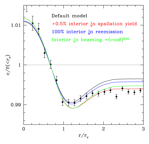
Figure 8: Variation of the model normalised neutron count rate profile with different changes to the default model for a $45$ km-radius crater (black line) relative to the LPNS epithermal neutron result for the stack of $40<r_{\rm c}/{\rm km}<50$ craters (points). The red curve shows the model resulting from increasing the emitted epithermal neutron flux per input cosmic ray by $0.5\%$ within the crater. Including reemission of all neutrons (rather than the default of none) from the crater interior surface changes the default model to that shown with a blue curve. The green line results from increasing the neutron beaming from the surface from $0.50$ to $0.51$ within the crater only.

Similar changes to the simple model are able to fit the thermal and epithermal neutron profiles for all crater size ranges. The required enhancement is $0.3-0.4\%$ for the crater subsets with $r_{\rm c}<50$ km, with this enhancement ranging out to $1.5-2r_{\rm c}$ from the crater centre.

One possible explanation for the enhanced neutron emission could be surface or near-surface roughness, of the sort seen by radar measurements out to twice the crater radius (Stickle et al., 2015). While previous neutron transport simulations for planetary surfaces have assumed emission from a flat surface (Lawrence et al., 2006), it has been shown that the neutron leakage flux can be enhanced for non-flat surfaces (Drüke and Schaal, 1991). If such roughness leads to the increase in emitted neutron flux required to fit the observed LPNS count rate profiles, then the neutron count rate could actually be sensitive to the physical condition of the lunar surface, making it complementary to the radar and thermal infrared data sets (Bandfield et al., 2011; Ghent et al., 2015). The impact of changing the regolith mass distribution near the surface can be addressed directly using Monte Carlo neutron transport simulations that use realistic topographic models of a planetary surface, as has been done for other planetary bodies (Prettyman and Hendricks, 2015).

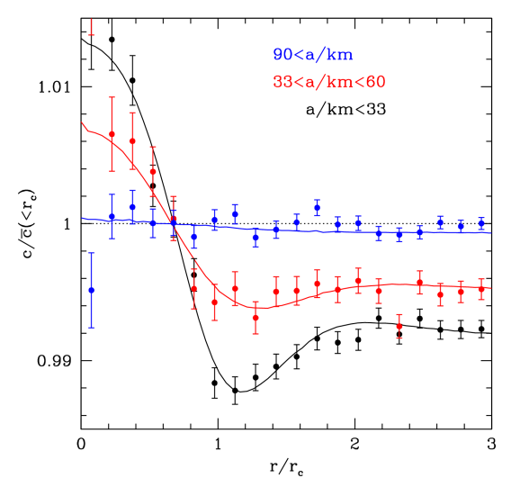
Figure 9: Stacked, normalised radial LP epithermal neutron count rate profiles for $40-50$ km radius craters as a function of LP altitude. Blue, black and red results correspond to detector altitudes of $a<33$ km, $[33,60]$ km and $a>90$ km respectively. Curves show the corresponding best-fitting model results.

6 Implications for hydrogen in polar cold traps

The beaming of neutrons increases the count rate measured by the LPNS when it passes over craters. This is the opposite effect to that produced by placing hydrogen into permanently shaded regions (PSRs) within polar craters, which reduces the epithermal count rate. Not accounting for the varying topography will lead to underestimates of the water-equivalent hydrogen cold-trapped into polar PSRs. If the change in observed count rate due to topography is $\sim 1\%$, then one might wonder how this could possibly have a significant impact upon the inferred WEH. However, this small change to the observed count rate is evident over the entire crater area, whereas the PSR may only cover a tiny fraction of the crater area. The blurring caused by the response function of the LPNS can have the effect of levering a small effect acting over the large crater area into a large effect in the small PSR area.

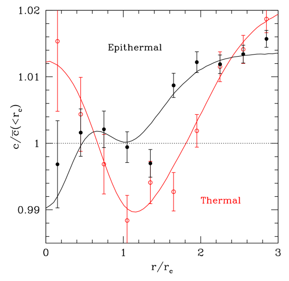
Figure 10: LP epithermal (black filled circles) and thermal (red open circles) neutron count rate profiles for Cabeus crater. Curves show models for an $r_{\rm c}=42$ km crater with the topography that best-fits that of Cabeus, and $75\%$ reemission of neutrons hitting the crater interior. The black curve additionally has a central “composition” that emits only $0.35$ times as many neutrons per cosmic ray as the rest of the surface. The red curve traces a model where the surface interior to $r_{\rm c}=2.2$ emits $0.97$ times as many neutrons per cosmic ray as the rest of the surface.

Rather than considering a general crater, it makes sense to focus on Cabeus, where LCROSS actually made a local estimate of the WEH weight percentage. Cabeus is also significantly deeper than the average crater with a similar radius. The azimuthally-averaged shape of Cabeus is best fitted with a profile defined by $d=6.05$ km, $x_{\rm i}/x_{\rm c}=0.7$, $x_{\rm e}/x_{\rm c}=2.3$ and $u=0.85$ km. Adopting $42$ km as the radius of the crater (Head et al., 2010), and choosing a central circular disc covering $275$ km² as the PSR (Teodoro et al., 2010), a model where the PSR region emits $0.35$ times as many epithermal neutrons per incoming cosmic ray as the rest of the surface gives rise to the black line in Figure 10. This reasonably fits the epithermal neutron data for Cabeus, shown with black filled circles. The thermal neutron data, in contrast, are well-fitted by a model where the surface interior to $2.2r_{\rm c}$ emits $0.97$ times as many neutrons as the rest of the surface.

That the thermal and epithermal count rate profiles differ is consistent with the suggestion that hydrogen in the PSR is responsible for the odd shape of the epithermal neutron profile, although the reason for the thermal neutron profile rising above $1$ at $r\mathrel{\hbox{\hbox to0.0pt{\hbox{\lower 4.0pt\hbox{$\sim$}}\hss}\hbox{$>$}}}2r_{\rm c}$ is not clear. If one ascribes the lack of an epithermal central count rate bump entirely to hydrogen in the PSR, then the factor of $0.35$ in neutron count rate can be converted using the formula supplied by Lawrence et al. (2006) into $\sim 4.5$ wt$\%$ WEH. This is a factor of four greater than was inferred by Teodoro et al. (2010), and consistent with the LCROSS results (Colaprete et al., 2010; Strycker et al., 2013). As Cabeus does not have a simple crater morphology and the possibility that additional compositional variation is being suggested by the thermal neutron profile, this value should be taken with a pinch of salt. However, it serves to illustrate how the effect of topography upon remotely-sensed neutron count rates could lead to a significant bias in the inferred wt$\%$ WEH. Given that many PSRs occupy a larger fraction of the area of the crater within which they reside, the case of Cabeus may be a more extreme example of how large an effect topography can play.

7 Conclusions

This study shows that there are some features in the neutron count rate profiles sensed from orbital detectors as they are flown over lunar craters located in highland regions. There is a central bump in the detected count rate, and the mean count rate over the stacked crater is up to $1\%$ larger than it is outside. This factor is largest for thermal and epithermal neutrons, but still detectable in the fast neutrons.

A simple geometrical model has been developed. It predicts qualitatively very similar behaviour to that observed from the LPNS thermal and epithermal data sets. The central peak results from the weak beaming of emitted neutrons normal to the surface (Lawrence et al., 2006), which is analogous to solar limb darkening. This simple model underestimates the mean count rate observed over the crater by $\sim 0.3\%$.

To fit the observed stacked count rate profiles well requires a $\sim 0.35\%$ enhancement in the neutron emissivity of the regolith within $\sim 2r_{\rm c}$ of the crater centre. It should be possible, using Monte Carlo neutron transport simulations, to determine if this can be achieved by a plausible amount of surface or near-surface roughness.

The beaming of neutrons over polar craters hosting PSRs may mean that the concentration of hydrogen in the PSRs has been underestimated in previous work. For the particular case of Cabeus, where a large crater contains a relatively small PSR, it was shown that $\sim 4.5$ wt$\%$ WEH within the PSR can reproduce the epithermal neutron count rate profile, assuming a simple azimuthally-symmetric topographical model for Cabeus. This is a factor of four times larger than previously inferred, and is consistent with the value measured using LCROSS data. In polar craters where the PSR occupies a larger fraction of the crater, the impact of topography on the inferred wt$\%$ WEH will be less important.

Appendix A Details of the model neutron count rate calculation

In order to calculate the model neutron count rate in an orbiting omni-directional detector, it is easiest to split the surface into a few distinct regions: the unperturbed surface, the outer uplifted slope, the crater walls and the flat infill region in the crater centre. The simpler case with no uplift will be considered first.

A.1 Neutron count rate from the uncratered surface

Figure 11: Variables used in the calculation of the count rate from the unperturbed lunar surface. The origin is placed at the lunar centre, O, and the detector, D, is at an altitude $a$ above the surface.

This part of the calculation is very similar to that described in Appendix B of Prettyman et al. (2006). The flux of neutrons a distance $r$ away from a patch of lunar surface of area d$A$, at an angle $\theta$ to the surface normal, as shown in Fig. 11, will satisfy

$${\rm d}f(r,\theta)\propto\frac{\cos^{1+\alpha}\theta}{r^{2}}\,{\rm d}A,$$ (11)

where $\alpha$ represents the effective beaming of neutrons from the surface. Integrating over $2\pi$ steradians and defining the flux through the surface as $f_{0}$, leads to

$${\rm d}f(r,\theta)=\frac{(2+\alpha)f_{0}}{2\pi r^{2}}\cos^{1+\alpha}\theta\,{\rm d}A.$$ (12)

The flux detected from the whole surface is then

$$f=\frac{(2+\alpha)f_{0}}{2\pi}\int_{0}^{2\pi}{\rm d}\phi\int_{0}^{\beta_{\rm max}}\left(\frac{r_{\rm m}}{r}\right)^{2}\cos^{1+\alpha}\theta\sin\beta~{}{\rm d}\beta.$$ (13)

As shown in Fig. 11, $\beta$ is the angle subtended at the lunar centre by the vectors to the detector and surface patch and $\beta_{\rm max}=\cos^{-1}[r_{\rm m}/(r_{\rm m}+a)]$ defines the lunar horizon for a detector at altitude $a$. Using the sine and cosine rules,

$$\sin\theta=\left(\frac{r_{\rm m}+a}{r}\right)\sin\beta,$$ (14)

and

$$r^{2}=(r_{\rm m}+a)^{2}+r_{\rm m}^{2}-2r_{\rm m}(r_{\rm m}+a)\cos\beta.$$ (15)

Defining $t=(r_{\rm m}+a)/r_{\rm m}$ yields

$$f=(2+\alpha)f_{0}\int_{0}^{\beta_{\rm max}}\frac{(t\cos\beta-1)^{1+\alpha}\sin\beta{\rm d}\beta}{(t^{2}+1-2t\cos\beta)^{\frac{3+\alpha}{2}}},$$ (16)

which can be computed numerically to find the flux from the uncratered surface.

Figure 12: Variables used in the calculation of the count rate from the unperturbed part of the surface when a crater is present. The dotted line represents the intersection of the cone with half-opening angle $\beta$ and the sphere with radius $r_{\rm m}$.

The detector has been assumed to be omni-directional in the above calculation such that the detected count rate is merely proportional to the flux at the detector. The LPNS is, in fact, cylindrical and thus is not quite omni-directional. However, comparison of the inferred instrumental point-spread function with that given by Maurice et al. (2004) shows them to be similar in shape to the extent that correcting for any differences has a negligible effect upon the results in this paper.

When a crater is inserted into the surface, the integration limits in equation (13) need to be changed. If the crater centre lies at the spacecraft nadir, then the minimum $\beta$ is increased so that the integration starts at the edge of the crater. However, for a more general crater position it is necessary to find the range of azimuthal angle $\phi$ that lies outside the crater as a function of $\beta$. Figure 12 shows this more general configuration, where the crater centre subtends an angle $\theta_{\rm cen}$ at the lunar centre. Without loss of generality, the detector and crater centre can both be placed in the $x-z$ plane, where the axes have been chosen such that the y axis is into the page and the detector is placed on the z axis. The required $\phi(\beta)$ can be found by determining the points where the ring of lunar surface at $\beta$ intersects with the plane containing the crater rim. Using the fact that the crater centre lies in the same plane as the crater rim, one can infer that the rim plane is given by

$$\underline{x}.\underline{\hat{n}}=r_{\rm cen}=r_{\rm m}\cos\theta_{c},$$ (17)

where the unit normal to the plane is given by

$$\underline{\hat{n}}=\left(\begin{array}[]{c}-\sin\theta_{\rm cen}\\ 0\\ \cos\theta_{\rm cen}\\ \end{array}\right).$$ (18)

Noting the symmetry in the y direction and finding the solution when

$$\underline{x}=r_{\rm m}\left(\begin{array}[]{c}\sin\beta\cos\phi\\ \sin\beta\sin\phi\\ \cos\beta\\ \end{array}\right),$$ (19)

leads to the following expression for $\phi_{rim}(\beta)$, the angle that represents the fraction of $\pi$ radians outside the crater for this $\beta$:

$$\cos\phi_{rim}=\frac{\cos\theta_{\rm cen}\cos\beta-\cos\theta_{c}}{\sin\theta_{\rm cen}\sin\beta}.$$ (20)

A.2 Cosmic ray occlusion within a crater

Figure 13: Variables used in the calculation of the sky visibility from a point P, at $y=0$, within the spherical cap crater. Points F and Q represent the crater focus and the point on the crater rim that lies in the vertical plane through P making an angle $\phi$ with the x axis. $\theta_{\rm max}(\phi)$ represents the maximum colatitude to which P sees cosmic rays at an angle $\phi$. $\eta$ is the angle between the x axis and the point underneath Q in the $x-y$ plane, such that tan$\eta=y_{Q}/x_{Q}$.

The cosmic ray flux impinging upon a unit area of crater interior will be lower than that incident on the outside, convex surface. Under the assumption that the cosmic ray flux is isotropic, this is accounted for by replacing $f_{0}$ with $f_{0}\Omega_{\rm i}/\pi$, where $\Omega_{\rm i}$ is the cos(incidence angle)-weighted solid angle of visible sky. At a point P within a spherical cap crater, this is given by

$$\Omega_{\rm i}=\int_{0}^{2\pi}\int_{0}^{\theta_{\rm max}(\phi)}\cos i\sin\theta~{}{\rm d}\theta{\rm d}\phi,$$ (21)

where the incidence angle, $i$, is the angle between the vector $\underline{\rm PF}$ and the direction $(\theta,\phi)$ and $\theta_{\rm max}$ is the maximum angle down from the $z$ direction that lies above the crater rim, as shown in Figure 13. Q represents the point on the crater rim at this particular azimuthal angle, $\phi$, and the vector $\underline{\rm PQ}$ makes an angle $\theta_{\rm max}$ with the z direction. The incidence angle can be written in terms of the two angular coordinates as

$$\cos i=\frac{(r_{\rm curv}-z_{P})\cos\theta-x_{P}\cos\phi\sin\theta}{r_{\rm curv}},$$ (22)

where $x_{P}$ and $z_{P}$ are the $x$ and $z$ coordinates of point P.

Redefining the origin of the coordinate system to be at the base of the crater, the position of Q is given by

$$\underline{x}_{Q}=\left(\begin{array}[]{c}x_{c}\cos\eta\\ x_{c}\sin\eta\\ d\\ \end{array}\right),$$ (23)

with $\eta$ being the angle between the x axis and the point beneath Q in the $z=0$ plane. Point P has coordinates

$$\underline{x}_{P}=\left(\begin{array}[]{c}x_{P}=r_{\rm curv}\sin\psi\\ 0\\ z_{P}=r_{\rm curv}(1-\cos\psi)\\ \end{array}\right),$$ (24)

where $\psi$ is the angle between the -z direction and FP. The vertical plane containing P and Q has

$$\underline{\hat{n}}=\left(\begin{array}[]{c}\sin\phi\\ -\cos\phi\\ 0\\ \end{array}\right),$$ (25)

and satisfies

$$\underline{x}.\underline{\hat{n}}=x_{P}\sin\phi.$$ (26)

Inserting $\underline{x}_{Q}$ into this equation yields the following expression for $\eta$ as a function of $\phi$:

$$\eta=\phi-\sin^{-1}\left(\frac{x_{P}}{x_{\rm c}}\sin\phi\right).$$ (27)

Using the fact that

$$\hat{\underline{\rm PQ}}.\hat{\underline{z}}=\cos\theta_{\rm max},$$ (28)

one can infer that

$$\cos\theta_{\rm max}=\frac{d-z_{P}}{\sqrt{x_{\rm c}^{2}+x_{P}^{2}-2x_{\rm c}x_{P}\cos\eta+(d-z_{P})^{2}}}.$$ (29)

For a choice of crater shape and distance from the crater axis, $x_{P}$, equations (27) and (29) determine $\cos\theta_{\rm max}(\phi)$, which can then be used in conjunction with equations (21) and (22) to determine the fraction of sky visible from this point within the crater.

Extending this approach to the case where there is a flat infilled region in the crater centre is straightforward. In practice, a table of $\Omega$ values as a function of $x_{P}$ is created once, and this is used, with interpolation, for the two-dimensional numerical integration to find the flux coming from within the crater.

A.3 Visibility of a surface patch from the detector

Out to the lunar horizon the crater exterior is all visible to the detector in the case where there is no uplifted rim. However, there are parts of the crater interior that may not be visible to the detector. Consequently, it is necessary to see if the line-of-sight from the detector to the surface patch passes above or below the crater rim.

Placing the origin of the coordinate system, O, at the lunar centre, and the detector at

$$\underline{x}_{D}=(r_{\rm m}+a)\left(\begin{array}[]{c}\sin\theta_{D}\\ 0\\ \cos\theta_{D}\\ \end{array}\right),$$ (30)

with the z axis going through the crater centre, a general point within the crater can be written as

$$\underline{x}_{P}=\left(\begin{array}[]{c}r_{\rm curv}\sin\psi\cos\gamma\\ r_{\rm curv}\sin\psi\sin\gamma\\ r_{\rm m}\cos\theta_{c}-d+r_{\rm curv}(1-\cos\psi)\\ \end{array}\right),$$ (31)

where $\gamma$ represents the angle around from the $x$ axis to point P. The symmetry of the problem means that the contribution to the flux coming from $0\leq\gamma\leq\pi$ is the same as that from $-\pi\leq\gamma\leq 0$. Following a similar methodology to that adopted in Section A.2, the normal to the plane containing O, P and D can be defined using $\underline{n}=\underline{x}_{P}\times(\underline{x}_{D}-\underline{x}_{P})$. The point Q on the rim determining if the detector is above or below the crater rim as viewed from P can then be found as the solution to $\underline{x}_{Q}.\underline{\hat{n}}=\underline{x}_{P}.\underline{\hat{n}}$ with an $x$ coordinate between those of P and D. In this case,

$$\underline{x}_{Q}=\left(\begin{array}[]{c}x_{c}\cos\eta\\ x_{c}\sin\eta\\ r_{\rm m}\cos\theta_{c}\\ \end{array}\right)$$ (32)

and the plane equation is used to determine $\eta$. For the detector to be able to see point P requires

$$\underline{\hat{z}}.\frac{(\underline{x}_{D}-\underline{x}_{P})}{|\underline{x}_{D}-\underline{x}_{P}|}>\underline{\hat{z}}.\frac{(\underline{x}_{Q}-\underline{x}_{P})}{|\underline{x}_{Q}-\underline{x}_{P}|}.$$ (33)

These equations, along with those from Sections A.1 and A.2, allow the computation of the curves in the top two panels of Figure 6. One and two dimensional numerical integrations are required to evaluate the flux from outside and within the crater respectively. For the flux from within the crater, it is also necessary to compute the distance to the detector and the angle between surface normal and the detector direction, but these are readily found from the vectors used to determine if the detector can see that point within the crater. The two dimensional integration to find the crater flux is simply done over an azimuthal angle ranging from $0$ to $2\pi$ and the angle from the focus to the crater centre, $\psi$, running from $0$ to $\psi_{\rm max}=\tan^{-1}[x_{\rm c}/(r_{\rm curv}-d)]$.

A.4 Uplifted crater rim

Including an uplifted crater rim complicates the calculation considerably, because parts of the previously unperturbed surface may now undergo some cosmic ray shadowing and may also no longer be visible from the detector. Similarly, the outer uplifted slope going from the crater rim back down to the unperturbed surface is a new topographical component that also suffers from these issues. In contrast, the calculation of the flux from the crater itself is only slightly changed to account for the raising of the entire crater surface.

A.4.1 Cosmic ray occlusion

Considering first the occlusion of cosmic rays from the outer uplifted slope and the unperturbed surface, the symmetry is such that this is just a function of the distance from the crater centre. The outer uplifted slope is most conveniently parametrised using an azimuthal angle, $\epsilon$ and the fraction of the way down the slope from the rim to the unperturbed surface, $f$. For a point P on the outer uplifted slope, the azimuthal variation of the maximum polar angle to which the sky can be seen, $\theta_{\rm max}(\phi)$, will be set either by the unperturbed surface or the outer uplifted slope, depending on which is hit first as the zenith angle increases.

Choosing the z axis to pass through point P and the crater centre to lie in the $x-z$ plane at $x<0$, the value of $\theta_{\rm max}$ to the unperturbed surface is independent of $\phi$. Simple trigonometry gives

$$\cos\theta_{{\rm max},1}=-\sqrt{1-\left(\frac{r_{\rm m}}{r_{P}}\right)^{2}},$$ (34)

with $r_{P}$ being the distance of point P from the lunar centre. For sufficiently extended outer slopes, it is possible for $r_{P}<r_{\rm m}$, in which case $\cos\theta_{{\rm max},1}$ is set to $0$.

It may be that the outer uplifted slope itself is the first piece of lunar surface to intersect the line-of-sight as the zenith angle is increased at a particular azimuthal angle. In this case, $\theta_{\rm max}$ is set by the local slope at point P in the azimuthal direction, $\phi$. For a small displacement on the uplifted slope having components d$x$ and d$y$, such that $({\rm d}s)^{2}=({\rm d}x)^{2}+({\rm d}y)^{2}$ and tan$\phi=\,$d$y/$d$x$, the maximum zenith angle to the outer uplifted slope can be found from

$$\cos\theta_{{\rm max},2}(\phi)=\sin\left[\tan^{-1}\left(\frac{{\rm d}z}{{\rm d}s}\right)\right].$$ (35)

$$\frac{{\rm d}z}{{\rm d}s}=\frac{\partial z}{\partial x}\frac{{\rm d}x}{{\rm d}s}+\frac{\partial z}{\partial y}\frac{{\rm d}y}{{\rm d}s},$$ (36)

with $\partial z/\partial y=0$, ${\rm d}s/{\rm d}x=1/\cos\phi$ and $\partial z/\partial x$ being the gradient $g$ from equation (6) rotated through $\theta_{\rm cen}$ into the coordinate system with P on the z axis. This leads to

$$\frac{\partial z}{\partial x}=\frac{\sin\theta_{\rm cen}+g\cos\theta_{\rm cen}}{\cos\theta_{\rm cen}-g\sin\theta_{\rm cen}}.$$ (37)

The value of $\cos\theta_{\rm max}(\phi)$ is taken as the larger of $\cos\theta_{{\rm max},1}$ and $\cos\theta_{{\rm max},2}(\phi)$, and the cosmic ray occlusion factor, $\Omega_{i}/\pi$, at a given fraction of the way down the outer uplifted slope is calculated using equation (21).

The cosmic ray occlusion for points on the unperturbed surface, like that on the outer uplifted slope, is just a function of distance to the crater centre. It is convenient to place the patch of unperturbed surface under consideration, P, on the $z$ axis and rotate the crater centre through an angle $-\theta_{\rm cen}$ about the $y$ axis (moving the crater in the $-x$ direction). Points an angle $\epsilon$ around from the $x$ axis on the crater rim, ${\underline{x}}_{R}$, or the outer edge of the outer uplifted slope, ${\underline{x}}_{E}$, can then be described via

$$\underline{x}_{R}=\left(\begin{array}[]{c}-(r_{m}\cos\theta_{c}+u)\sin\theta_{\rm cen}+r_{\rm m}\sin\theta_{c}\cos\epsilon\cos\theta_{\rm cen}\\ r_{m}\sin\theta_{c}\sin\epsilon\\ (r_{\rm m}\cos\theta_{c}+u)\cos\theta_{\rm cen}+r_{\rm m}\sin\theta_{c}\cos\epsilon\sin\theta_{\rm cen}\\ \end{array}\right)$$ (38)

and

$$\underline{x}_{E}=\left(\begin{array}[]{c}-r_{m}\cos\theta_{e}\sin\theta_{\rm cen}+r_{\rm m}\sin\theta_{e}\cos\epsilon\cos\theta_{\rm cen}\\ r_{m}\sin\theta_{e}\sin\epsilon\\ r_{\rm m}\cos\theta_{e}\cos\theta_{\rm cen}+r_{\rm m}\sin\theta_{e}\cos\epsilon\sin\theta_{\rm cen}\\ \end{array}\right)$$ (39)

respectively. For a given azimuthal angle $\phi$ around from the $x$ axis as seen from point P on the z axis, it is possible to find any points on the uplifted outer slope that lie in the plane

$$[\underline{x}_{R}+f(\underline{x}_{E}-\underline{x}_{R})].\left(\begin{array}[]{c}\sin\phi\\ -\cos\phi\\ 0\\ \end{array}\right)=0.$$ (40)

If there are no solutions for $f$ in the range [0,1], then the plane at fixed $\phi$ does not intersect the uplifted region and $\cos\theta_{\rm max}(\phi)=0$. If solutions exist, then equation (40) provides a constraint on $f(\epsilon)$ for points on the outer uplifted slope that lie in the plane an azimuthal angle $\phi$ around from the x axis as viewed from point P on the unperturbed surface. The largest zenith angle from which cosmic rays arrive at point P, $\theta_{\rm max}(\phi)$, is found using a numerical minimisation algorithm applied to the set of points on the slope. A root-finding algorithm is employed to determine $f$ at any given $\epsilon$ as part of this process. Given $\cos\theta_{\rm max}(\phi)$ as a function of distance from the crater centre, the cosmic ray occlusion factors can be found using equation (21).

A.4.2 Visibility of surface patch from detector

Points on either the outer uplifted slope or the unperturbed surface may not be visible from the detector as a result of the uplifted region surrounding the crater.

For a point P on the outer uplifted slope to be visible from the detector, D, the line of sight must not be blocked by either the outer uplifted slope or the unperturbed surface. If the dot product of the surface normal at P and the surface-to-detector vector, $\underline{\Delta}=\underline{x}_{D}-\underline{x}_{P}$, is positive, then P is not blocked by the outer uplifted slope. The unperturbed surface will block the line-of-sight if the line connecting P to the detector passes within $r_{\rm m}$ of the lunar centre. Defining the fractional distance along this line as $v$, such that $\underline{x}=\underline{x}_{P}+v\underline{\Delta}$, this happens if $0<v_{\rm min}<1$ and $|\underline{x}(v_{\rm min})|<r_{\rm m}$, where $v_{\rm min}$ represents the $v$ for which this line passes nearest to the lunar centre. With the coordinate system origin at the lunar centre, this leads to

$$v_{\rm min}=-\frac{\underline{x}_{P}.\underline{\Delta}}{|\underline{\Delta}|^{2}}$$ (41)

and

$$\frac{|\underline{x}(v_{\rm min})|^{2}}{r_{\rm m}^{2}}=\frac{|\underline{x}_{P}|^{2}-(\underline{x}_{P}.\underline{\hat{\Delta}})^{2}}{r_{\rm m}^{2}},$$ (42)

where $\underline{\hat{\Delta}}$ is a unit vector in the direction of $\underline{\Delta}$. These equations allow a quick determination of whether or not the unperturbed surface blocks the detector’s view of a part of the outer uplifted slope.

To determine the visibility of the unperturbed surface from the detector, consider placing the detector on the $z$ axis at $(0,0,r_{\rm m}+a)$ and the crater centre in the $x-z$ plane at $x\leq 0$. If the far point of the edge of the crater outer uplifted slope is visible above the far point of the rim ($\epsilon=\pi$ in equations (39) and  (38) respectively), then the entire unperturbed surface is visible from the detector. If this is not the case, then the plane containing the lunar centre, detector and point P can be found. The line of intersection of this plane with the uplifted slope and the minimum zenith angle from P to points on this line follow, and the visibility is determined by comparison with the zenith angle from point P to the detector. This is a very similar methodology to that described to determine the cosmic ray occlusion factor for the unperturbed surface.

A.5 Neutron flux impinging upon the crater walls

In the preceding sections of this appendix, the assumption has been made that any neutrons emitted from within the crater and aimed at the crater walls are absorbed on contact with the regolith and do not contribute to the neutron flux emerging from the crater. This is a simplification, because some of these neutrons will be re-emitted before being absorbed. The more energetic neutrons may even lead to nuclear reactions that create more than one lower energy neutron that escapes from the crater, in which case the crater would be producing a thermal neutron flux that was an amplified version of the incident fast neutron flux.

While quantifying the impact of this process requires Monte Carlo neutron transport simulations, it is possible to use the simple model to determine how much of the emitted crater flux impinges on the crater surface as a function of position within the crater. Following the methodology of the previous sections, when the crater flux at the detector was determined, it is possible to place the ‘detector’ on the crater surface and calculate the flux from the crater that is aimed into the crater surface. The only additional factor to consider is to include the fact that the normal to the ‘detecting’ surface is at different angles to the lines-of-sight to the various other bits of crater surface. Multiplying the detected flux by the cosine of the incidence angle and integrating over the entire crater surface leads to the results shown in Fig. 8 for the case where all neutrons are assumed to be reemitted from the surface.