Law of the wall in an unstably stratified turbulent channel flow

Abstract

We perform direct numerical simulations of an unstably stratified turbulent channel flow to address the effects of buoyancy on the boundary layer dynamics and mean field quantities. We systematically span a range of parameters in the space of friction Reynolds number ($Re_{\tau}$) and Rayleigh number ($Ra$). Our focus is on deviations from the logarithmic law of the wall due to buoyant motion. The effects of convection in the relevant ranges are discussed providing measurements of mean profiles of velocity, temperature and Reynolds stresses as well as of the friction coefficient. A phenomenological model is proposed and shown to capture the observed deviations of the velocity profile in the log-law region from the non-convective case.

1 Introduction

Wall bounded turbulence is highly relevant to a variety of engineering systems and naturally occurring flows. As such, the importance of the fundamental understanding of the generation of turbulent fluctuations by fluid-solid interactions in the boundary layers and their transport and interaction with the bulk mean flow (Pope, 2001) is evident. In many geophysical and industrial flows, shear flows and wall turbulence are subjected to either stable or unstable thermal stratifications. When gravity and/or temperature differences are strong enough, buoyancy forces may alter significantly the boundary layer dynamics. Stable stratification is known to inhibit the bursting phenomenon, i.e. depleting the transport of turbulent fluctuations from the wall to the bulk, thus reducing the turbulent drag and increasing the mean flow velocity. Many studies have been devoted to this situation when the stratified scalar field is passive (Johansson & Wikström, 1999; Papavassiliou & Hanratty, 1997) and active (Armenio & Sarkar, 2002; Gerz, Schumann & Elgobashi, 1989; Iida, Kasagi & Nagano, 2002; García-Villalba & del Álamo, 2011) and even in presence of non-Oberbeck-Boussinesq effects (Zonta, Onorato & Soldati, 2012).

The unstable configuration is also relevant in a variety of instances, such as the physics of the atmospheric layer superposed to an over-heated ground (as, e.g., in summer days, determining the generation of thermo-convective storms (Bluestein, 2013)). Early theoretical results on turbulent boundary layers under unstable thermal stratification date back to Prandtl (1932) who pioneered a mixing-length based approach which inspired the later work of Obukhov (1946) anticipating the Monin-Obukhov similarity theory (henceforth MO54) (Monin & Obukhov, 1954). These pioneering works have boosted a number of experimental (Lenschow, 1970; Businger et al, 1971; Kaimal et al, 1982; Hunt, Kaimal & Gaynor, 1988) and numerical (Deardroff, 1972, 1974; Moeng, 1984) works, as well as further theoretical developments based either on $k-\varepsilon$ theories (Mellor & Yamada, 1974, 1982) or on the Rapid Distortion Theory (RDT) (Dubrulle et al, 2002a, b) on the dynamics of planetary boundary layers (PBL). Also, in another seminal paper, Kader & Yaglom (1990) revised MO54 and compared it with experimental data. Lumley, Zeman & Siess (1978) proposed an eddy-damped quasi-Gaussian closure able to predict the inversion regions of heat flux profiles in strongly buoyant sheared boundary layers. Numerical results (Iida & Kasagi, 1997) and experimental flume measurements (combined with a spectral equation model) (Komori et al, 1982) showed that natural thermal convection affects the mechanisms of momentum and heat transport from the wall and tends to flatten the velocity profile in the bulk; these observation were confirmed by large-eddy simulations of a variable density fluid (Zainali & Lessani, 2010), although with non-Boussinesq effects, as, e.g. profile asymmetries emerging at large stratifications.

In this work we perform direct numerical simulations based on the lattice Boltzmann (hereafter LB) method of an unstably (thermally) stratified turbulent channel flow. Our focus is on identifying the effects of buoyancy on the channel flow structure by comparing profiles of mean fields and fluctuations over a wide range of parameters with a pure (unstratified) channel flow. Our results show a decreased fluid throughput due to a strongly flattened velocity profile, which could, however, be fitted by a log-law with coefficients depending on the input controlling parameters (friction Reynolds number $Re_{\tau}$ and Rayleigh number $Ra$, defined below), as also derived theoretically.

2 Numerical method and simulation details

We simulated a fluid enclosed between two walls, kept at fixed temperatures $T_{H}$ at $y=0$ and $T_{C}=T_{H}-\Delta$ at $y=2H$, and driven by a constant body force mimicking an imposed pressure gradient along the streamwise direction $\hat{x}$. The equations of motion are the incompressible Navier-Stokes equation for the fluid velocity field $\bm{u}(\bm{x},t)$ in the Boussinesq approximation (namely, the density is assumed to be constant $\rho=\rho_{0}$, but for the linearised buoyancy term)

$$\partial_{t}\bm{u}+\bm{u}\cdot\bm{\nabla}\bm{u}=-\bm{\nabla}P+\nu\triangle\bm{u}-\beta\bm{g}(T-T_{m})+\bm{F},$$ (1)

($T_{m}=(T_{H}+T_{C})/2$ being the mean temperature) coupled with the advection-diffusion equation for the temperature field $T(\bm{x},t)$

$$\partial_{t}T+\bm{u}\cdot\bm{\nabla}T=\alpha\triangle T.$$ (2)

In the above equations, $P$ is the pressure field (rescaled by $\rho_{0}$), $\bm{g}=-g\hat{y}$ is the acceleration of gravity and $\bm{F}=(u_{\tau}^{2}/H)\hat{x}$ is the acceleration due to the constant body force ($u_{\tau}$ being the friction velocity); $\nu$, $\alpha$ and $\beta$ are the kinematic viscosity, the thermal diffusivity and thermal expansion coefficient, respectively. As a numerical scheme, we adopted a 3d LB algorithm (Benzi, Succi & Vergassola, 1992; Chen & Doolen, 1998; Aidun & Clausen, 2010) with two probability densities (for density/momentum and for temperature, respectively) (He, Chen & Doolen, 1998). The method has been extensively used to study both thermal convection (Benzi, Toschi & Tripiccione, 1998; Calzavarini, Toschi & Tripiccione, 2002) and turbulent channel flow (Toschi et al, 1999; Toschi, Lévêque & Ruiz-Chavarría, 2000; Biferale et al, 2002); in particular Lavezzo, Clercx & Toschi (2011) validated the code and tested grid resolutions against previous studies with different numerical methods.

We used a computational grid $L\times 2H\times W$ of $256\times 128\times 128$ lattice points, with each run longer than $3\times 10^{6}$ time steps (in LB units), in such a way to achieve statistically steady states of $\sim 200T_{L}$ ($T_{L}$ being the large-scale eddy turnover time). From equations (1) and (2) two dimensionless groups can be identified giving rise to two parameters which control the dynamics, namely the shear (or friction) Reynolds number,

$$Re_{\tau}=\frac{u_{\tau}H}{\nu}$$

and the Rayleigh number

$$Ra=\frac{\beta g\Delta(2H)^{3}}{\nu\alpha}$$

quantifying, respectively, the strength of the pressure induced shear and of the buoyancy with respect to viscous dissipation.

We performed turbulent channel flow simulations with $Re_{\tau}\in[46,205]$; for each $Re_{\tau}$ we tuned the gravity (at fixed temperature jump), whence the buoyancy, spanning the range $Ra\in[0,1.3\times 10^{7}]$. The Prandtl number $Pr=\nu/\alpha$ is equal to one in all cases presented.

3 Results

Mean profiles of the streamwise velocity $U(y)=\overline{u_{x}}$ (the overline indicates here and henceforth averaging over planes parallel to the walls $\overline{(\cdot)}=(L_{x}L_{z})^{-1}\int(\cdot)dxdz$) in the channel are shown in figure 1. For each Reynolds number ($Re_{\tau}=130$ and $Re_{\tau}=205$) we show data from simulations at three different Rayleigh numbers ($Ra=8.12\times 10^{5}$, $Ra=6.5\times 10^{6}$ and $Ra=1.3\times 10^{7}$), besides the unstratified channel flow ($Ra=0$). An evident effect of thermal stratification is a decrease of the centreline velocity and a flattening of the profiles at increasing $Ra$; indeed, mixing between the bulk and the boundary layer regions due to wall-normal thermal fluctuations (or “plumes”) results in an increase of the effective wall drag (Hattori, Morita & Nagano, 2006). Such effects are more pronounced for lower $Re_{\tau}$, as it clearly appears by comparison of left and right panels of figure 1. These observations will be discussed more quantitatively under the light of the modelling in the next section.

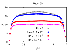
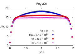
Figure 1: Mean profiles of the streamwise velocity $U(y)$, normalized with the friction velocity $u_{\tau}$, for various Rayleigh numbers ($Ra=0$, $Ra=8.12\times 10^{5}$, $Ra=6.5\times 10^{6}$ and $Ra=1.3\times 10^{7}$) at fixed shear Reynolds number $Re_{\tau}$. Left: $Re_{\tau}=130$, Right: $Re_{\tau}=205$. The data have been plotted every two points (i.e. lattice spacings) for the sake of clarity of visualisation

Figure 2 shows the mean temperature profile with respect to $y$, for the same cases displayed in figure 1. Here, we note the bending of the thermal profiles in the bulk with increased shear Reynolds number, in contrast to the thermal shortcut observed in pure turbulent Rayleigh-Bénard (solid line in the right panel) (Ahlers, Grossmann & Lohse, 2009; Chillà & Schumacher, 2012), owing to the destruction or sweeping of the coherent plumes rising from the wall surfaces (Scagliarini, Gylfason & Toschi, 2014).

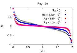
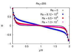
Figure 2: Mean profiles of the normalized temperature $\Theta=2(T-T_{m})/\Delta$ as a function of the height $y$ for various Rayleigh numbers ($Ra=0$, $Ra=8.12\times 10^{5}$, $Ra=6.5\times 10^{6}$ and $Ra=1.3\times 10^{7}$) at fixed shear Reynolds number $Re_{\tau}$. Left: $Re_{\tau}=130$, Right: $Re_{\tau}=205$; the solid line represents the profile for the purely convective Rayleigh-Bénard case (i.e. $Re_{\tau}=0$) with $Ra=8.12\times 10^{5}$. The data have been plotted every two points (i.e. lattice spacings) for the sake of clarity of visualisation

Longitudinal and transverse mean squared components of the fluctuating velocity field (hereafter $\tilde{u}_{i}=u_{i}-\overline{u}_{i}$) are shown in figure 3 for the same cases as in figure 1 (normalized with the friction velocity). When the fluctuating quantities are concerned, most notably the lateral component is increased in the bulk region, and as the Rayleigh number is increased, the magnitude becomes comparable or greater than the stream-wise component. The near wall regions are also affected, primarily in the streamwise component, where an increase and a subsequent decrease in magnitude is observed as the Rayleigh number is increased.

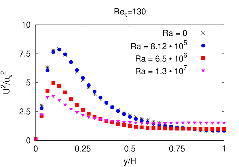
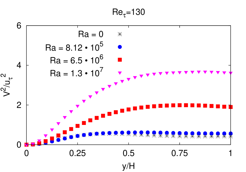
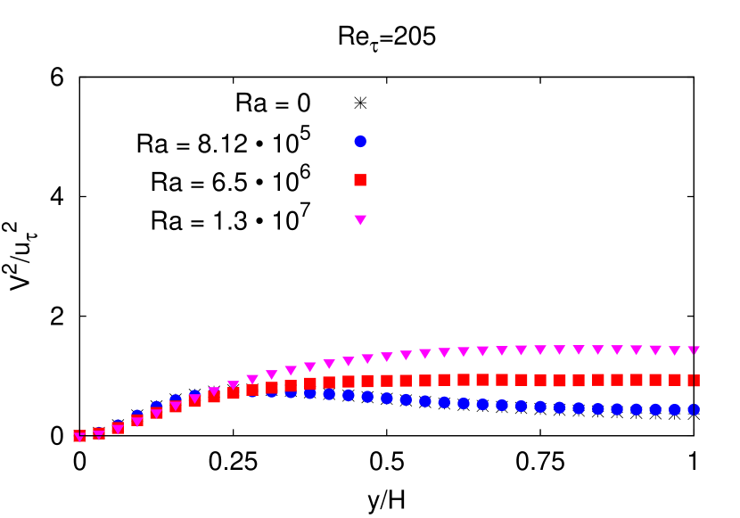
Figure 3: Profiles of longitudinal $U^{2}=\overline{\tilde{u}_{x}^{2}}$ and transverse $V^{2}=\overline{\tilde{u}_{y}^{2}}$ mean squared components of the fluctuating velocity field, normalized by the friction velocity $u_{\tau}$ for various Rayleigh numbers ($Ra=0$, $Ra=8.12\times 10^{5}$, $Ra=6.5\times 10^{6}$ and $Ra=1.3\times 10^{7}$) at fixed shear Reynolds number $Re_{\tau}$.

In order to quantify the overall effect of the thermal forcing on the channel flow, figure 4 shows the skin-friction coefficient $c_{f}=\tau_{w}/(1/2U_{0}^{2})$ as a function of shear Reynolds number $Re_{\tau}$. The increased drag due to the thermal field is evident, resulting in higher than usual friction coefficient. The effect is reduced asymptotically, as the Reynolds number is increased for a given Rayleigh number, emphasizing that shear becomes the dominant source of turbulence at sufficiently high Reynolds numbers.

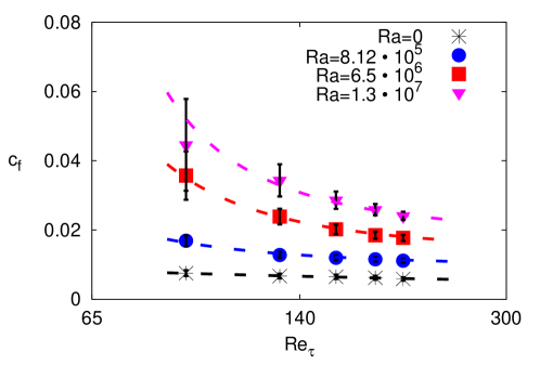
Figure 4: The skin-friction coefficient $c_{f}=\tau_{w}/(1/2U_{0}^{2})$ as a function of the shear Reynolds number $Re_{\tau}$ for various Rayleigh numbers $Ra$. The dashed lines are predictions obtained by approximating the mean velocity by a log-law over the whole channel; for the stratified cases we made use of equations (3)-(4) with the same fitting parameter $C_{s}=2.5$ for all $Ra$ (see section 4.)

4 Modification of the law of the wall by buoyancy

Inspection of the profiles of the mean quantities and the fluctuations showed that buoyancy alters the channel flow structure. We now focus on the mean velocity profiles. In figure 5 we report the lin-log plot of profiles, in wall units, for $Re_{\tau}=185$ and for various $Ra$. Convective motion, realised in the form of thermal plumes rising from the walls to the bulk, disturbs the coherence of the channel flow, resulting in a source of drag which decreases the mean velocity in the channel and hence the mass throughput, as well as flattening the velocity profile.

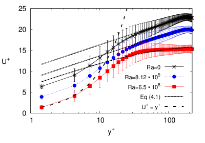
Figure 5: Lin-log plot of the velocity profiles in wall units, for shear Reynolds number $Re_{\tau}=185$ and Rayleigh numbers $Ra=0$ ($\ast$), $Ra=8.12\times 10^{5}$ ($\bullet$) and $Ra=6.5\times 10^{6}$ ($\blacksquare$); the data are shifted vertically for clarity of visualisation. The dashed lines indicate the linear law, valid in the viscous layer, $U^{+}=y^{+}$, while the dash-dotted ones correspond to the prediction (3)-(4) with $\kappa=0.42$, $C_{S}=2.5$ and $B\in[5.8,6.7]$.

In order to quantify these observations, in the following we attempt to generalize von Kármán’s law of the wall accounting for buoyancy effects. To this aim, we propose a simple model constructed from conservation laws and phenomenological arguments, which predicts that the viscous buffer is insensitive to buoyancy (i.e. $U^{+}=y^{+}$), while in the log-law region the following relation

$$U^{+}(y^{+})=\kappa^{-1}\log\left(\frac{y^{+}}{1+\kappa_{C}y^{+}}\right)+B,$$ (3)

holds (quantities have been expressed in wall units $U^{+}\equiv U/u_{\tau}$ and $y^{+}\equiv y/\delta$, with $\delta=\nu/u_{\tau}$). In equation (3), $\kappa$ is the von Kármán constant, $B$ is an integration constant and $\kappa_{C}$ is given by

$$\kappa_{C}(Ra,Re_{\tau})=C_{S}\frac{Ra}{Re_{\tau}^{4}Pr^{2}};$$ (4)

$C_{S}$ is a phenomenological parameter. All profiles in figure 5 agree reasonably, within error bars, with our predictions: the data collapse on the function $U^{+}=y^{+}$ for $y^{+}<10$ (dashed lines) while in the logarithmic layer they can be fitted with equation (3) (dash-dotted lines), whose derivation is detailed in what follows.
Applying the Reynolds decomposition $\bm{u}(\bm{x},t)=U(y)\hat{x}+\tilde{\bm{u}}(\bm{x},t)$ for the velocity field and averaging the Navier-Stokes equation for the $\hat{x}$ velocity component, we get, upon integration in $y$, an exact relation (Pope, 2001) between the mean shear $S(y)=dU(y)/dy$ and the Reynolds stress $\tau_{xy}(y)=-\overline{\tilde{u}_{x}\tilde{u}_{y}}$ namely:

$$\nu S(y)+\tau_{xy}(y)=u_{\tau}^{2}\left(1-\frac{y}{H}\right),$$ (5)

or, in wall units:

$$S^{+}(y^{+})+\tau^{+}_{xy}(y^{+})=\left(1-\frac{y^{+}}{Re_{\tau}}\right).$$ (6)

Notice that equations (5)-(6) remain valid also in the presence of buoyancy, since the forcing term $\beta g(T-T_{m})\hat{y}$ does not act along the streamwise direction. For very large $Re_{\tau}$ (in principle $Re_{\tau}\rightarrow\infty$), equation (6) gives $S^{+}+\tau^{+}_{xy}=1$; close to the wall (for $y^{+}<10$), where viscous terms dominate, $S^{+}\gg\tau^{+}_{xy}$ whence $S^{+}\approx 1$ which implies $U^{+}\simeq y^{+}$, as anticipated above. Conversely, away from the wall (typically for $y^{+}\stackrel{{\scriptstyle>}}{{\sim}}30$), turbulent fluctuations dominate over viscous processes and $\tau^{+}_{xy}\gg S^{+}$, i.e. (L’vov et al, 2004)

$$\tau^{+}_{xy}\approx const;$$ (7)

such result alone, however, does not give any further insight on the behaviour of the velocity profile in the corresponding region of the channel. To this aim, we need to consider the budget equation of turbulent kinetic energy $E_{K}(y)=\overline{|\tilde{\bm{u}}|^{2}}/2$ (Pope, 2001). In the log-law layer the energy production $\mathcal{P}=\tau_{xy}(y)S(y)+\beta gQ(y)$ (where $Q(y)=\overline{u_{y}\theta}$ is the turbulent heat flux and $\theta$ are the temperature fluctuations) is balanced by dissipation $\varepsilon(y)=2\nu\overline{(\partial_{i}\tilde{u}_{j})^{2}}$ (Pope, 2001); the latter cannot be calculated exactly but only inferred by means of phenomenological arguments: for large Reynolds number and outside the viscous boundary layer, the dissipation equals the turbulent energy flux, which can be estimated as $E_{K}(y)/\tau(y)$, where $\tau(y)\propto y/\sqrt{E_{K}(y)}$ is the typical eddy turn-over time at $y$ (L’vov et al, 2004). Thus, the energy balance equation reads:

$$\frac{aE_{K}^{3/2}(y)}{y}=\tau_{xy}(y)S(y)+\beta gQ(y),$$ (8)

where $a$ is a non-dimensional parameter of order unity.

Equation (8) is not yet closed: a relation between $E_{K}(y)$ and $\tau_{xy}(y)$ is required. Dimensional analysis suggests that the two quantities should be proportional to each other, i.e. $E_{K}(y)\propto\tau_{xy}(y)$ (L’vov et al, 2004); such assumption can be readily tested in the numerical simulations: in the main panel of figure 6 we show that the ratio $E_{K}(y)/\tau_{xy}(y)$, indeed, approaches a constant value for $y^{+}\stackrel{{\scriptstyle>}}{{\sim}}40$.

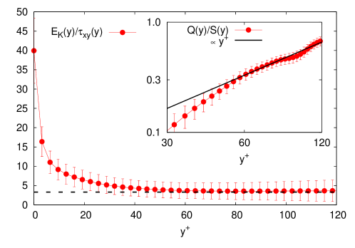
Figure 6: Main panel: Ratio of the turbulent kinetic energy $E_{K}$ over the Reynolds stress $\tau_{xy}$ (for the case $Re_{\tau}=205$, $Ra=8.12\times 10^{5}$): the plateau attained for $y^{+}\stackrel{{\scriptstyle>}}{{\sim}}40$ suggests that the two quantities are proportional to each other in the log-law region. Inset: Ratio of the turbulent heat flux $Q(y)$ over the mean shear $S(y)$; the solid line indicates a linear dependence on $y^{+}$ and represents a numerical check of the validity of the assumptions leading to equation (13).

We can then rewrite (8) as (in view also of (7))

$$\frac{a(E_{K})^{3/2}}{y}=cE_{K}S(y)+\beta gQ(y),$$ (9)

with $c$ yet another dimensionless number. The energy production by buoyancy term, viz. the heat flux, needs also to be modelled; although more refined closures can be employed (Johansson & Wikström, 1999; Hattori, Morita & Nagano, 2006) involving tensorial eddy diffusivities and coupling with gradients of the temperature field in all directions, we adopt a simple standard mixing length ansatz, i.e.

$$Q(y)=\overline{u_{y}\theta}=-\ell_{m}^{2}\partial_{y}\overline{U}\partial_{y}\overline{T}.$$ (10)

A first order closure like (10) must not be expected to work well for second order quantities like temperature fluctuations, Reynolds stresses, etc, but, as we will show, mean streamwise velocity profiles are satisfactorily reproduced through such model; according to Prandtl’s hypothesis the mixing length $\ell_{m}$ is proportional to the distance from the wall, i.e. $\ell_{m}\propto y$, whence

$$Q(y)=\overline{u_{y}\theta}=-by^{2}\partial_{y}\overline{U}\partial_{y}\overline{T},$$ (11)

where $b$ is a numerical constant. The mean temperature gradient will, in principle, depend itself on the shear profile; however, in a perturbative spirit, we postulate here, for simplicity, a logarithmic form, such that

$$\frac{d\overline{T}}{dy}=-\frac{T_{*}}{y},$$ (12)

where $T_{*}=\frac{\alpha\Delta}{2H\,u_{\tau}}$ is a scale for the dynamic temperature. The functional form (12) somehow interpolates between the passive scalar case (Johansson & Wikström, 1999) and the natural convection (Ahlers et al, 2012) and it is in agreement with a theoretical prediction based on RDT (Dubrulle et al, 2002b). Inserted in the expression for the heat flux (11), equation (12) gives

$$Q(y)\propto by^{2}S(y)\frac{T_{*}}{y}=b^{\prime}yS(y)T_{*}.$$ (13)

For the sake of validation of our arguments, we check equation (13) (which predicts $Q(y)\propto yS(y)$) against the numerics in the inset of figure 6, finding a reasonably good agreement. Inserting (13) into (9) provides

$$\frac{a(E_{K})^{3/2}}{y}=cE_{K}S(y)+\beta gb^{\prime}yS(y)\frac{\alpha\Delta}{2Hu_{\tau}},$$

which can be recast, introducing the wall units and the definitions of $Re_{\tau}$ and $Ra$, in the following form

$$\frac{1}{\kappa y^{+}}=S^{+}\left(1+C_{S}\frac{Ra}{Pr^{2}Re_{\tau}^{4}}y^{+}\right);$$ (14)

it must be noticed that the two parameters $\kappa$ and $C_{S}$ are combinations of dimensionless quantities emerging in the derivation, which cannot be, however, derived from first principles; fits of the numerical data indicate that good estimates are the values $\kappa=0.42$ and $C_{S}=2.5$. Explicitating the shear term in (14), we get

$$\frac{dU^{+}}{dy^{+}}=\frac{1}{\kappa y^{+}(1+\kappa_{C}y^{+})},$$ (15)

whose integration finally yields expressions (3) and (4) for the velocity profile. The robustness of the model is confirmed in figure 7 where we plot the fitted values of the parameter $\kappa_{C}$ as function of $Ra$ for fixed $Re_{\tau}$ (main panel) and as function of $Re_{\tau}$ for fixed $Ra$ (inset), together with the predictions of equation (4) (dashed lines).

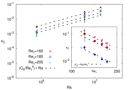
Figure 7: Plots of the parameter $\kappa_{C}(Ra,Re_{\tau})$ of the model as function of $Ra$ for fixed $Re_{\tau}$’s (main panel) and as function of $Re_{\tau}$ for fixed $Ra$’s (inset), whose values are $Ra=8.12\cdot 10^{5}$ ($\bullet$), $Ra=6.5\cdot 10^{6}$ ($\blacksquare$) and $Ra=1.3\cdot 10^{7}$ ($\blacktriangledown$). The dashed lines represent equation (4) with constant $C_{S}$ fixed at $C_{S}=2.5$ for all cases.

Before concluding, we assimilate our results, mutatis mutandis, to those obtained in the literature for PBL. Our setup differs from PBL in that we simulate a channel flow with fixed temperature (and zero velocity) at the two walls; unlike the classical MO54 approach (Monin & Obukhov, 1954; Dyer, 1974), then, as written in equations (10) and (13), we do not assume the heat flux to be constant as a sort of boundary condition (Monin & Obukhov, 1954) (which is an approximation, as pointed out in Mellor & Yamada (1982)). However, some analogies might be considered. With respect to other models (Dubrulle et al, 2002b; Mellor & Yamada, 1982), our approach enjoys some peculiar features: $\left.i\right)$ it relies on one single empirical input (the parameter $C_{S}$); $\left.ii\right)$ it provides an explicit analytic expression for the velocity profile and for its dependence on $Ra$, $Re_{\tau}$ and $Pr$, which makes it particularly suitable for comparison against data from channel flow simulations where one has direct control on these parameters. On the other hand, our model must not be expected to be fully trustable for high values of the stability parameter $\zeta=y/L_{O}$, where $L_{O}=u_{\tau}^{3}/(\kappa\beta gQ_{w})$ is the Obukhov length (Monin & Obukhov, 1954) and $Q_{w}$ the heat flux at the wall. For a further comparison, it is worth rewriting equation (15) in terms of the dimensionless mean wind gradient $\phi_{U}$ as

$$\phi_{U}(y)\equiv\frac{\kappa y}{u_{\tau}}\frac{dU}{dy}=\left(1+C_{S}\frac{y}{L_{S}}\right)^{-1},$$ (16)

where the characteristic length $L_{S}$ is defined as

$$L_{S}=\frac{Re_{\tau}^{3}Pr^{2}}{Ra}H.$$ (17)

If we introduce the Nusselt number $Nu=Q_{w}/(\alpha\Delta/2H)$, the Obukhov length $L_{O}$, in turn, can be expressed in terms of $(Ra,Re_{\tau},Pr)$ as

$$L_{O}=\frac{16}{\kappa}\frac{H}{Nu}\frac{Re_{\tau}^{3}Pr^{2}}{Ra}\approx\frac{16}{\kappa}\lambda_{\theta}\frac{Re_{\tau}^{3}Pr^{2}}{Ra},$$ (18)

where $\lambda_{\theta}$ is the boundary layer width (the last equality is only approximated since, as mentioned before, in certain cases there is no clear thermal shortcut (Grossmann & Lohse, 2000)). A direct look at equations (17) and (18) suggests that

$$L_{O}\propto\frac{\lambda_{\theta}}{H}L_{S},$$

but $\lambda_{\theta}$ is fixed by the heat flux from the wall and, hence, it depends in a non-trivial way on the control parameters. In the form (16-17), our model appears, then, as an equivalent similarity theory for unstably stratified turbulent channel flows. Furthermore, the expression of the Obukhov length $L_{O}$ (18) in terms of the controlling parameters allows us to check the consistency of our data, in the logarithmic layer, with previous theoretical studies (Dubrulle et al, 2002b) and, by consequence, with experimental data (Businger et al, 1971).

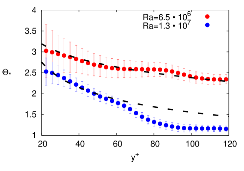
Figure 8: Temperature fluctuations $\Theta_{*}\equiv\overline{(T-\overline{T})^{2}}^{1/2}/(Q_{w}/u_{\tau})$ from our LB simulations (symbols) and RDT prediction (19), with the expression (18) for $L_{O}$, (dashed lines) as function of the wall-normal direction coordinate in wall units (the range shown is restricted to the logarithmic layer). The data have been fitted with the theoretical curves using for the parameters $(\alpha_{1},\alpha_{2})$ the values: ($0.26$,$0.6$), for $Ra=6.5\times 10^{6}$, and ($0.22$,$0.9$), for $Ra=1.3\times 10^{7}$.

In figure 8 we compare the temperature fluctuations $\Theta_{*}\equiv\overline{(T-\overline{T})^{2}}^{1/2}/(Q_{w}/u_{\tau})$ from our simulations with the RDT prediction (Dubrulle et al, 2002b):

$$\Theta_{*}^{(RDT)}(\zeta)=\frac{1}{(\alpha_{1}+\alpha_{2}\zeta)}.$$ (19)

The numerical data and the theoretical result (dashed line) appear to be in fair agreement, within error bars; in particular, the dependence on $(Ra,Re_{\tau})$ as in (18) is fulfilled.

5 Conclusions

We have studied, by means of direct numerical simulations based on a thermal lattice Boltzmann algorithm, the dynamics of a turbulent channel flow under a gravity field orthogonal to the streamwise direction coupled to an imposed temperature difference between the top (cold) wall and the bottom (hot) wall. The resulting unstably stratified configuration flattens the velocity profile and decreases the centreline value when the buoyancy strength is increased. This effective drag shows up in an enhancement of the friction coefficient. The action of buoyancy on the boundary layer structure has also been probed looking at other relevant statistical quantities in wall bounded turbulent system, such as Reynolds stress; we have found that, as the Rayleigh number is increased, the squared wall normal velocity grows in the bulk becoming comparable or even larger than the streamwise component (which, in turn, is depleted close to the wall). To provide a quantitative interpretation of the numerical findings, we have proposed a phenomenological model resulting in a modified logarithmic law of the boundary layer; such model could successfully capture the various velocity profiles at changing the shear Reynolds and Rayleigh number, with just one adjustable parameter.
AS, HE and AG acknowledge financial support from the Icelandic Research Fund. AS acknowledges funding from the European Research Council under the EU Seventh Framework Programme (FP7/2007-2013) / ERC Grant Agreement no[279004]. This work was partially supported by the Foundation for Fundamental Research on Matter (FOM), a part of the Netherlands Organisation for Scientific Research (NWO), and by the COST action MP1305.

References

- Ahlers et al (2012) Ahlers G., Bodenschatz E., Funfschilling D., Grossmann S., He X., Lohse D., Stevens R.J.A.M. & Verzicco R. 2012 Logarithmic temperature profiles in turbulent Rayleigh-Bénard convection. Phys. Rev. Lett. 109, 114501.
- Ahlers, Grossmann & Lohse (2009) Ahlers G., Grossmann S. & Lohse D. 2009 Heat transfer and large scale dynamics in turbulent Rayleigh-Bénard convection. Rev. Mod. Phys. 81, 503-537.
- Aidun & Clausen (2010) Aidun C.K. & Clausen J.R. 2010 Lattice Boltzmann Method for complex flows. Annu. Rev. Fluid Mech. 42, 439-472.
- Armenio & Sarkar (2002) Armenio V. & Sarkar S. 2002 An investigation of stably stratified turbulent channel flow using large-eddy simulation. J. Fluid Mech. 459, 1-42.
- Benzi, Succi & Vergassola (1992) Benzi R., Succi S. & Vergassola M. 1992 The lattice Boltzmann equation: theory and applications. Phys. Rep. 222, 145-197.
- Benzi, Toschi & Tripiccione (1998) Benzi R., Toschi F., & Tripiccione R. 1998 On the heat transfer in Rayleigh–Bénard systems. J. Stat. Phys. 93, 901.
- Biferale et al (2002) Biferale L., Lohse D., Mazzitelli I. & Toschi F. 2002 Probing structures in channel flow through SO(3) and SO(2) decomposition. J. Fluid Mech. 452, 39-59.
- Bluestein (2013) Bluestein H.B. 2013 Severe convective storms and tornadoes, Springer.
- Businger et al (1971) Businger J.A., Wyngaard J.C., Izumi Y. & Bradley E.F. 1971 Flux profile relationships in the atmospheric surface layer. J. Atmos. Sci. 28, 181-189.
- Calzavarini, Toschi & Tripiccione (2002) Calzavarini E., Toschi F., & Tripiccione R. 2002 Evidences of Bolgiano-Obhukhov scaling in three-dimensional Rayleigh-Bénard convection. Phys. Rev. E 66, 016304.
- Chen & Doolen (1998) Chen S. & Doolen G.D. 1998 Lattice Boltzmann Method for fluid flows. Annu. Rev. Fluid Mech. 30, 329-364.
- Deardroff (1972) Deardroff J.W. 1972 Numerical investigation of neutral and unstable planetary boundary layers, J. Atmos. Sci. 29, 91–115.
- Deardroff (1974) Deardroff J.W. 1974 Three dimensional numerical study of turbulence in an entraining mixed layer, Boundary Layer Meteorol. 7, 199-226.
- Dubrulle et al (2002a) Dubrulle B., Laval J.-P., Sullivan P.P. & Werne J. 2002a A new dynamical subgrid model for the planetary surface layer. Part I: The model and a priori tests. J. Atmos. Sci. 59, 861-876.
- Dubrulle et al (2002b) Dubrulle B., Laval J.-P., Sullivan P.P. & Werne J. 2002b A new dynamical subgrid model for the planetary surface layer. Part II: Analytical computation of fluxes, mean profiles, and variances, J. Atmos. Sci. 59, 877-891.
- Dyer (1974) Dyer A.J. 1974 A review of flux-profile relationships, Boundary Layer Meteorol. 7, 363-372.
- García-Villalba & del Álamo (2011) García-Villalba M & del Álamo J.C. 2011 Turbulence modification by stable stratification in channel flow. Phys. Fluids 23, 045104.
- Gerz, Schumann & Elgobashi (1989) Gerz T., Schumann U. & Elgobashi S.E. 1989 Direct numerical simulation of stratified homogeneous turbulent shear flows. J. Fluid Mech. 200, 563-594.
- Grossmann & Lohse (2000) Grossmann S. & Lohse D. 2011 Scaling in thermal convection: a unifying theory. J. Fluid Mech. 407, 27-56.
- Hattori, Morita & Nagano (2006) Hattori H., Morita A. & Nagano Y. 2006 Nonlinear eddy diffusivity models reflecting buoyancy effect for wall-shear flows and heat transfer. Int. J. Heat Mass Transfer 27, 671-683.
- He, Chen & Doolen (1998) He X., Chen S. & Doolen G.D. 1998 A novel thermal model for the Lattice Boltzmann Method in incompressible limit. J. Comp. Phys. 146, 282-300.
- Hunt, Kaimal & Gaynor (1988) Hunt J.C.R., Kaimal J.C. & Gaynor J.E. 1988 Eddy structure in the convective boundary layer-new measurements and new concepts. Q. J. R. Meteorol. Soc. 114, 827-858.
- Iida & Kasagi (1997) Iida O. & Kasagi N. 1997 Direct numerical simulation of unstably stratified turbulent channel flow. J. Heat Transfer - Trans. ASME 119, 53-61.
- Iida, Kasagi & Nagano (2002) Iida O., Kasagi N. & Nagano Y. 2002 Direct numerical simulation of turbulent channel flow under stable density stratification. Int. J. Heat Mass Transfer 45, 1693-1703.
- Johansson & Wikström (1999) Johansson A.V. & Wikström P.M. 1999 DNS and modelling of passive scalar transport in turbulent channel flow with a focus on scalar dissipation rate modelling. Flow, Turbulence and Combustion 63, 223-245.
- Kader & Yaglom (1990) Kader B.A. & Yaglom A.M. 1990 Mean fields and fluctuations moments in unstably stratified turbulent boundary layers. J. Fluid Mech. 212, 637-662.
- Kaimal et al (1982) Kaimal J.C., Eversole R.A., Lenschow D.H., Stankov B.B., Kahn P.H. & Businger J.A. 1982 Spectral characteristics of the convective boundary layer over uneven terrain. J. Atmos. Sci. 39, 1098–1114.
- Komori et al (1982) Komori S., Ueda H., Ogino F. & Mizushina T. 1982 Turbulence structure in unstably-stratified open-channel flow. Phys. Fluids 25, 1539-1546.
- Lenschow (1970) Lenschow D. J. 1970 Airplane measurements of planetary boundary layer structure. J. Appl. Meteorol. 9, 874-884.
- L’vov et al (2004) L’vov V.S., Pomyalov A., Procaccia I. & Tiberkevich V. 2004 Drag reduction by polymers in wall bounded turbulence. Phys. Rev. Lett. 92, 244503.
- Lumley, Zeman & Siess (1978) Lumley J.L., Zeman O. & Siess J. 1978 The influence of buoyancy on turbulent transport. J. Fluid Mech. 84, 581-597.
- Mellor & Yamada (1974) Mellor G.L. & Yamada T. 1974 A hierarchy of turbulence closure models for planetary boundary layers. J. Atmos. Sci. 41, 1791-1806.
- Mellor & Yamada (1982) Mellor G.L. & Yamada T. 1982 Development of a turbulence closure model for geophysical gluid problems. Rev. Geophys. Space Phys. 20, 851-875.
- Moeng (1984) Moeng C.-H. 1984 A Large-Eddy-Simulation model for the study of planetary boundary-layer turbulence. J. Atmos. Sci. 41, 2052–2062.
- Monin & Obukhov (1954) Monin A.S. & Obukhov A.M. 1954 Basic laws of turbulent mixing in the atmospheric boundary layer Trudy Inst. Teor. Geofiz. Akad. Nauk SSSR 24, 163-187.
- Obukhov (1946) Obukhov A.M. 1946 Turbulence in thermally inhomogeneous atmosphere. Trudy Inst. Teor. Geofiz. Akad. Nauk SSSR 1, 95-115.
- Papavassiliou & Hanratty (1997) Papavassiliou D.V. & Hanratty T.J. 1997 Transport of a passive scalar in a turbulent channel flow. Int. J. Heat Mass Transfer 40, 1303-1311.
- Pope (2001) Pope S.B. 2001 Turbulent flows, Cambridge University Press.
- Prandtl (1932) Prandtl L. 1932 Meteorologische Anwendung der Strömungslehre. Beitr. Phys. fr. Atmos. 19, 188-202.
- Procaccia, L’vov & Benzi (2008) Papavassiliou D.V. & Hanratty T.J. 2008 Theory of drag reduction by polymers in wall-bounded turbulence. Rev. Mod. Phys. 80, 225-247.
- Scagliarini, Gylfason & Toschi (2014) Scagliarini A., Gylfason A., & Toschi F. 2014 Heat-flux scaling in turbulent Rayleigh-Bénard convection with an imposed longitudinal wind. Phys. Rev. E. 89, 043012.
- Chillà & Schumacher (2012) Chillà F. & Schumacher J. 2012 New perspectives in turbulent Rayleigh-Bénard convection. Eur. Phys. J. E 35, 58.
- Toschi et al (1999) Toschi F., Amati G., Succi S., Benzi R. & Piva R. 1999 Intermittency and structure functions in channel flow turbulence. Phys. Rev. Lett. 82, 5044.
- Toschi, Lévêque & Ruiz-Chavarría (2000) Toschi F., Lévêque E. & Ruiz-Chavarría G. 2000 Shear effects in nonhomogeneous turbulence. Phys. Rev. Lett. 85, 1436.
- Lavezzo, Clercx & Toschi (2011) Lavezzo V., Clercx H.J.H. & Toschi F. 2011 Rayleigh-Bénard convection via Lattice Boltzmann method: code validation and grid resolution effects. J. Phys.: Conf. Ser. 333, 012011.
- Zainali & Lessani (2010) Zainali A. & Lessani B. 2010 Large-eddy simulations of unstably stratified turbulent channel flow with high temperature differences. Int. J. Heat Mass Transfer 53, 4865-4875.
- Zonta, Onorato & Soldati (2012) Zonta F., Onorato M. & Soldati A. 2012 Turbulence and internal waves in stably-stratified channel flow with temperature-dependent fluid properties. J. Fluid Mech. 697, 175-203.