Universality for the pinning model in the weak coupling regime

Abstract.

We consider disordered pinning models, when the return time distribution of the underlying renewal process has a polynomial tail with exponent $\alpha\in(\frac{1}{2},1)$. This corresponds to a regime where disorder is known to be relevant, i.e. to change the critical exponent of the localization transition and to induce a non-trivial shift of the critical point. We show that the free energy and critical curve have an explicit universal asymptotic behavior in the weak coupling regime, depending only on the tail of the return time distribution and not on finer details of the models. This is obtained comparing the partition functions with corresponding continuum quantities, through coarse-graining techniques.

1. Introduction and motivation

Understanding the effect of disorder is a key topic in statistical mechanics, dating back at least to the seminal work of Harris [26]. For models that are disorder relevant, i.e. for which an arbitrary amount of disorder modifies the critical properties, it was recently shown in [12] that it is interesting to look at a suitable continuum and weak disorder regime, tuning the disorder strength to zero as the size of the system diverges, which leads to a continuum model in which disorder is still present. This framework includes many interesting models, including the 2d random field Ising model with site disorder, the disordered pinning model and the directed polymer in random environment (which was previously considered by Alberts, Quastel and Khanin [2, 1]).

Heuristically, a continuum model should capture the properties of a large family of discrete models, leading to sharp predictions about the scaling behavior of key quantities, such free energy and critical curve, in the weak disorder regime. The goal of this paper is to make this statement rigorous in the context of disordered pinning models [20, 21, 14], sharpening the available estimates in the literature and proving a form of universality. Although we stick to pinning models, the main ideas have a general value and should be applicable to other models as well.

In this section we give a concise description of our results, focusing on the critical curve. Our complete results are presented in the next section. Throughout the paper we use the conventions $\mathbb{N}=\{1,2,3,\ldots\}$ and $\mathbb{N}_{0}=\mathbb{N}\cup\{0\}$, and we write $a_{n}\sim b_{n}$ to mean $\lim_{n\to\infty}a_{n}/b_{n}=1$.

To build a disordered pinning model, we take a Markov chain $(S=(S_{n})_{n\in\mathbb{N}_{0}},\mathrm{P})$ starting at a distinguished state, called $0$, and we modify its distribution by rewarding/penalizing each visit to $0$. The rewards/penalties are determined by a sequence of i.i.d. real random variables $(\omega=(\omega_{n})_{n\in\mathbb{N}},\mathbb{P})$, independent of $S$, called disorder variables (or charges). We make the following assumptions.

• The return time to $0$ of the Markov chain $\tau_{1}:=\min\{n\in\mathbb{N}:\ S_{n}=0\}$ satisfies

  $$\mathrm{P}\left(\tau_{1}<\infty\right)=1,\qquad K(n):=\mathrm{P}\left(\tau_{1}=n\right)\sim\frac{L(n)}{n^{1+\alpha}},\quad n\to\infty,$$ (1.1)

  where $\alpha\in(0,\infty)$ and $L(n)$ is a slowly varying function [8]. For simplicity we assume that $K(n)>0$ for all $n\in\mathbb{N}$, but periodicity can be easily dealt with (e.g. $K(n)>0$ iff $n\in 2\mathbb{N}$).

• The disorder variables have locally finite exponential moments:

  $$\exists\beta_{0}>0:\ \Lambda(\beta):=\log\mathbb{E}(e^{\beta\omega_{1}})<\infty,\ \forall\beta\in(-\beta_{0},\beta_{0}),\qquad\mathbb{E}(\omega_{1})=0,\qquad\mathbb{V}(\omega_{1})=1\,,$$ (1.2)

  where the choice of zero mean and unit variance is just a convenient normalization.

Given a $\mathbb{P}$-typical realization of the sequence $\omega=(\omega_{n})_{n\in\mathbb{N}}$, the pinning model is defined as the following random probability law $\mathrm{P}_{\beta,h,N}^{\omega}$ on Markov chain paths $S$:

$$\frac{\mathrm{d}\mathrm{P}_{\beta,h,N}^{\omega}}{\mathrm{d}\mathrm{P}}(S):=\frac{e^{\sum_{n=1}^{N}(\beta\omega_{n}-\Lambda(\beta)+h)\mathds{1}_{\{S_{n}=0\}}}}{\mathrm{Z}_{\beta,h}^{\omega}(N)},\qquad\mathrm{Z}_{\beta,h}^{\omega}(N):=\mathrm{E}\Big{[}e^{\sum_{n=1}^{N}(\beta\omega_{n}-\Lambda(\beta)+h)\mathds{1}_{\{S_{n}=0\}}}\Big{]}\,,$$ (1.3)

where $N\in\mathbb{N}$ represents the “system size” while $\beta\geq 0$ and $h\in\mathbb{R}$ tune the disorder strength and bias. (The factor $\Lambda(\beta)$ in (1.3) is just a translation of $h$, introduced so that $\mathbb{E}[e^{\beta\omega_{n}-\Lambda(\beta)}]=1$.)

Fixing $\beta\geq 0$ and varying $h$, the pinning model undergoes a localization/delocalization phase transition at a critical value $h_{c}(\beta)\in\mathbb{R}$: the typical paths $S$ under $\mathrm{P}_{\beta,h,N}^{\omega}$ are localized at $0$ for $h>h_{c}(\beta)$, while they are delocalized away from $0$ for $h<h_{c}(\beta)$ (see (2.10) below for a precise result).

It is known that $h_{c}(\cdot)$ is a continuous function, with $h_{c}(0)=0$ (note that for $\beta=0$ the disorder $\omega$ disappears in (1.3) and one is left with a homogeneous model, which is exactly solvable). The behavior of $h_{c}(\beta)$ as $\beta\to 0$ has been investigated in depth [22, 3, 15, 4, 13], confirming the so-called Harris criterion [26]: recalling that $\alpha$ is the tail exponent in (1.1), it was shown that:

• for $\alpha<\frac{1}{2}$ one has $h_{c}(\beta)\equiv 0$ for $\beta>0$ small enough (irrelevant disorder regime);

• for $\alpha>\frac{1}{2}$, on the other hand, one has $h_{c}(\beta)>0$ for all $\beta>0$. Moreover, it was proven [25] that disorder changes the order of the phase transition: free energy vanishes for $h\downarrow h_{c}(\beta)$ at least as fast as $(h-h_{c}(\beta))^{2}$, while for $\beta=0$ the critical exponent is $\max(1/\alpha,1)<2$. This case is therefore called relevant disorder regime;

• for $\alpha=\frac{1}{2}$, known as the “marginal” case, the answer depends on the slowly varying function $L(\cdot)$ in (1.1): more precisely one has disorder relevance if and only if $\sum_{n}\frac{1}{n\,(L(n))^{2}}=\infty$, as recently proved in [7] (see also [4, 22, 23] for previous partial results).

In the special case $\alpha>1$, when the mean return time $\mathrm{E}[\tau_{1}]$ is finite, one has (cf. [6])

$$\lim\limits_{\beta\to 0}\,\frac{h_{c}(\beta)}{\beta^{2}}=\frac{1}{2\mathrm{E}[\tau_{1}]}\frac{\alpha}{1+\alpha}\,.$$ (1.4)

In this paper we focus on the case $\alpha\in(\frac{1}{2},1)$, where the mean return time is infinite: $\mathrm{E}[\tau_{1}]=\infty$. In this case, the precise asymptotic behavior of $h_{c}(\beta)$ as $\beta\to 0$ was known only up to non-matching constants, cf. [3, 15]: there is a slowly varying function $\tilde{L}_{\alpha}$ (determined explicitly by $L$ and $\alpha$) and constants $0<c<C<\infty$ such that for $\beta>0$ small enough

$$c\,\tilde{L}_{\alpha}\big{(}\tfrac{1}{\beta}\big{)}\,\beta^{\frac{2\alpha}{2\alpha-1}}\leq h_{c}(\beta)\leq C\,\tilde{L}_{\alpha}\big{(}\tfrac{1}{\beta}\big{)}\,\beta^{\frac{2\alpha}{2\alpha-1}}.$$ (1.5)

Our key result (Theorem 2.4 below) shows that this relation can be made sharp: there exists $m_{\alpha}\in(0,\infty)$ such that, under mild assumptions on the return time and disorder distributions,

$$\lim\limits_{\beta\to 0}\,\frac{h_{c}(\beta)}{\tilde{L}_{\alpha}(\frac{1}{\beta})\,\beta^{\frac{2\alpha}{2\alpha-1}}}=m_{\alpha}.$$ (1.6)

Let us stress the universality value of (1.6): the asymptotic behavior of $h_{c}(\beta)$ as $\beta\to 0$ depends only on the tail of the return time distribution $K(n)=\mathrm{P}(\tau_{1}=n)$, through the exponent $\alpha$ and the slowly varying function $L$ appearing in (1.1) (which determine $\tilde{L}_{\alpha}$): all finer details of $K(n)$ beyond these key features disappear in the weak disorder regime. The same holds for the disorder variables: any admissible distribution for $\omega_{1}$ has the same effect on the asymptotic behavior of $h_{c}(\beta)$.

Unlike (1.4), we do not know the explicit value of the limiting constant $m_{\alpha}$ in (1.6), but we can characterize it as the critical parameter of the continuum disordered pinning model (CDPM) recently introduced in [11, 12]. The core of our approach is a precise quantitative comparison between discrete pinning models and the CDPM, or more precisely between the corresponding partition functions, based on a subtle coarse-graining procedure which extends the one developed in [9, 10] for the copolymer model. This extension turns out to be quite subtle, because unlike the copolymer case the CDPM admits no “continuum Hamiltonian”: although it is built over the $\alpha$-stable regenerative set (which is the continuum limit of renewal processes satisfying (1.1), see §5.2), its law is not absolutely continuous with respect to the law of the regenerative set, cf. [11]. As a consequence, we need to introduce a suitable coarse-grained Hamiltonian, based on partition functions, which behaves well in the continuum limit. This extension of the coarse-graining procedure is of independent interest and should be applicable to other models with no “continuum Hamiltonian”, including the directed polymer in random environment [1].

Overall, our results reinforce the role of the CDPM as a universal model, capturing the key properties of discrete pinning models in the weak coupling regime.

2. Main results

2.1. Pinning model revisited

The disordered pinning model $\mathrm{P}_{\beta,h,N}^{\omega}$ was defined in (1.3) as a perturbation of a Markov chain $S$. Since the interaction only takes place when $S_{n}=0$, it is customary to forget about the full Markov chain path, focusing only on its zero level set

$$\tau=\{n\in\mathbb{N}_{0}:\ S_{n}=0\},$$

that we look at as a random subset of $\mathbb{N}_{0}$. Denoting by $0=\tau_{0}<\tau_{1}<\tau_{2}<\ldots$ the points of $\tau$, we have a renewal process $(\tau_{k})_{k\in\mathbb{N}_{0}}$, i.e. the random variables $(\tau_{j}-\tau_{j-1})_{j\in\mathbb{N}}$ are i.i.d. with values in $\mathbb{N}$. Note that we have the equality $\{S_{n}=0\}=\{n\in\tau\}$, where we use the shorthand

$$\{n\in\tau\}:=\bigcup_{k\in\mathbb{N}_{0}}\{\tau_{k}=n\}.$$

Consequently, viewing the pinning model $\mathrm{P}_{\beta,h,N}^{\omega}$ as a law for $\tau$, we can rewrite (1.3) as follows:

$$\frac{\mathrm{d}\mathrm{P}_{\beta,h,N}^{\omega}}{\mathrm{d}\mathrm{P}}(\tau):=\frac{e^{\sum_{n=1}^{N}(\beta\omega_{n}-\Lambda(\beta)+h)\mathds{1}_{\{n\in\tau\}}}}{\mathrm{Z}_{\beta,h}^{\omega}(N)},\qquad\mathrm{Z}_{\beta,h}^{\omega}(N):=\mathrm{E}\Big{[}e^{\sum_{n=1}^{N}(\beta\omega_{n}-\Lambda(\beta)+h)\mathds{1}_{\{n\in\tau\}}}\Big{]}\,.$$ (2.1)

To summarize, henceforth we fix a renewal process $(\tau=(\tau_{k})_{k\in\mathbb{N}_{0}},\mathrm{P})$ satisfying (1.1) and an i.i.d. sequence of disorder variables $(\omega=(\omega_{n})_{n\in\mathbb{N}},\mathbb{P})$ satisfying (1.2). We then define the disordered pinning model as the random probability law $\mathrm{P}_{\beta,h,N}^{\omega}$ for $\tau$ defined in (2.1).

In order to prove our results, we need some additional assumptions. We recall that for any renewal process satisfying (1.1) with $\alpha\in(0,1)$, the following local renewal theorem holds [18, 16]:

$$u(n):=\mathrm{P}(n\in\tau)\sim\frac{C_{\alpha}}{L(n)\,n^{1-\alpha}},\quad n\to\infty,\qquad\text{with}\ \ C_{\alpha}:=\frac{\alpha\sin(\alpha\pi)}{\pi}\,.$$ (2.2)

In particular, if $\ell=o(n)$, then $u(n+\ell)/u(n)\to 1$ as $n\to\infty$. We are going to assume that this convergence takes place at a not too slow rate, i.e. at least a power law of $\frac{\ell}{n}$, as in [11, eq. (1.7)]:

$$\exists\,C,n_{0}\in(0,\infty);\,\epsilon,\delta\in(0,1]:\quad\left|\frac{u(n+\ell)}{u(n)}-1\right|\leq C\left(\frac{\ell}{n}\right)^{\delta},\quad\forall n\geq n_{0},\,0\leq\ell\leq\epsilon n.$$ (2.3)

Remark 2.1.

This is a mild assumption, as discussed in [11, Appendix B]. For instance, one can build a wide family of nearest-neighbor Markov chains on $\mathbb{N}_{0}$ with $\pm 1$ increments (Bessel-like random walks) satisfying (1.1), cf. [5], and in this case (2.3) holds for any $\delta<\alpha$.

Concerning the disorder distribution, we strengthen the finite exponential moment assumption (1.2), requiring the following concentration inequality:

$$\begin{split}\exists\gamma>1,C_{1},C_{2}\in(0,\infty):\text{ for all $n\in\mathbb{N}$ and for all }f:\mathbb{R}^{n}\to\mathbb{R}\text{ convex and $1$-Lipschitz}\\ \mathbb{P}\Big{(}\big{|}f(\omega_{1},\ldots,\omega_{n})-M_{f}\big{|}\geq t\Big{)}\leq C_{1}\exp\bigg{(}-\frac{t^{\gamma}}{C_{2}}\bigg{)}\,,\qquad\quad\end{split}$$ (2.4)

where $1$-Lipschitz means $|f(x)-f(y)|\leq|x-y|$ for all $x,y\in\mathbb{R}^{n}$, with $|\cdot|$ the usual Euclidean norm, and $M_{f}$ denotes a median of $f(\omega_{1},\ldots,\omega_{n})$. (One can equivalently take $M_{f}$ to be the mean $\mathbb{E}[f(\omega_{1},\ldots,\omega_{n})]$ just by changing the constants $C_{1},C_{2}$, cf. [28, Proposition 1.8].)

It is known that (2.4) holds under fairly general assumptions, namely:

• ($\gamma=2$)  if $\omega_{1}$ is bounded, i.e. $\mathbb{P}(|\omega_{1}|\leq a)=1$ for some $a\in(0,\infty)$, cf. [28, Corollary 4.10];

• ($\gamma=2$)  if the law of $\omega_{1}$ satisfies a log-Sobolev inequality, in particular if $\omega_{1}$ is Gaussian, cf. [28, Theorems 5.3 and Corollary 5.7]; more generally, if the law of $\omega_{1}$ is absolutely continuous with density $\exp(-U-V)$, where $U$ is uniformly strictly convex (i.e. $U(x)-cx^{2}$ is convex, for some $c>0$) and $V$ is bounded, cf. [28, Theorems 5.2 and Proposition 5.5];

• ($\gamma\in(1,2)$)  if the law of $\omega_{1}$ is absolutely continuous with density given by $c_{\gamma}\,e^{-|x|^{\gamma}}$ (see Propositions 4.18 and 4.19 in [28] and the following considerations).

2.2. Free energy and critical curve

The normalization constant $\mathrm{Z}_{\beta,h}^{\omega}(N)$ in (2.1) is called partition function and plays a key role. Its rate of exponential growth as $N\to\infty$ is called free energy:

$$\mathrm{F}(\beta,h):=\lim_{N\to\infty}\frac{1}{N}\log\mathrm{Z}_{\beta,h}^{\omega}(N)=\lim_{N\to\infty}\frac{1}{N}\mathbb{E}\Big{[}\log\mathrm{Z}_{\beta,h}^{\omega}(N)\Big{]},\qquad\mathbb{P}\text{-a.s. \ and in \ }L^{1},$$ (2.5)

where the limit exists and is finite by super-additive arguments [20, 14]. Let us stress that $\mathrm{F}(\beta,h)$ depends on the laws of the renewal process $\mathrm{P}(\tau_{1}=n)$ and of the disorder variables $\mathbb{P}(\omega_{1}\in\mathrm{d}x)$, but it does not depend on the $\mathbb{P}$-typical realization of the sequence $(\omega_{n})_{n\in\mathbb{N}}$. Also note that $h\mapsto\mathrm{F}(\beta,h)$ inherits from $h\mapsto\log\mathrm{Z}_{\beta,h}^{\omega}(N)$ the properties of being convex and non-decreasing.

Restricting the expectation defining $\mathrm{Z}_{\beta,h}^{\omega}(N)$ to the event $\{\tau_{1}>N\}$ and recalling the polynomial tail assumption (1.1), one obtains the basic but crucial inequality

$$\mathrm{F}(\beta,h)\geq 0\quad\forall\beta\geq 0,h\in\mathbb{R}.$$ (2.6)

One then defines the critical curve by

$$h_{c}(\beta):=\sup\{h\in\mathbb{R}:\ \mathrm{F}(\beta,h)=0\}.$$ (2.7)

It can be shown that $0<h_{c}(\beta)<\infty$ for $\beta>0$, and by monotonicity and continuity in $h$ one has

$$\mathrm{F}(\beta,h)=0\ \ \text{if}\ \ h\leq h_{c}(\beta),\qquad\mathrm{F}(\beta,h)>0\ \ \text{if}\ \ h>h_{c}(\beta).$$ (2.8)

In particular, the function $h\mapsto\mathrm{F}(\beta,h)$ is non-analytic at the point $h_{c}(\beta)$, which is called a phase transition point. A probabilistic interpretation can be given looking at the quantity

$$\ell_{N}:=\sum_{n=1}^{N}\mathds{1}_{\{n\in\tau\}}=\big{|}\tau\cap(0,N]\big{|},$$ (2.9)

which represents the number of points of $\tau\cap(0,N]$. By convexity, $h\mapsto\mathrm{F}(\beta,h)$ is differentiable at all but a countable number of points, and for pinning models it can be shown that it is actually $C^{\infty}$ for $h\neq h_{c}(\beta)$ [24]. Interchanging differentiation and limit in (2.5), by convexity, relation (2.1) yields

$$\text{for $\mathbb{P}$-a.e. $\omega$},\qquad\lim_{N\to\infty}\mathrm{E}_{\beta,h,N}^{\omega}\bigg{[}\frac{\ell_{N}}{N}\bigg{]}=\frac{\partial\mathrm{F}(\beta,h)}{\partial h}\ \begin{cases}=0&\text{if }h<h_{c}(\beta)\\ >0&\text{if }h>h_{c}(\beta)\end{cases}\,.$$ (2.10)

This shows that the typical paths of the pinning model are indeed localized at $0$ for $h>h_{c}(\beta)$ and delocalized away from $0$ for $h<h_{c}(\beta)$. We refer to [20, 21, 14] for details and for finer results.

2.3. Main results

Our goal is to study the asymptotic behavior of the free energy $\mathrm{F}(\beta,h)$ and critical curve $h_{c}(\beta)$ in the weak coupling regime $\beta,h\to 0$.

Let us recall the recent results in [12, 11], which are the starting point of our analysis. Consider any disordered pinning model where the renewal process satisfies (1.1), with $\alpha\in(\frac{1}{2},1)$, and the disorder satisfies (1.2). If we let $N\to\infty$ and simultaneously $\beta\to 0$, $h\to 0$ as follows:

$$\beta=\beta_{N}:=\hat{\beta}\frac{L(N)}{N^{\alpha-\frac{1}{2}}},\qquad h=h_{N}:=\hat{h}\frac{L(N)}{N^{\alpha}},\qquad\text{for fixed }\hat{\beta}>0,\ \hat{h}\in\mathbb{R}\,,$$ (2.11)

the family of partition functions $\mathrm{Z}_{\beta_{N},h_{N}}^{\omega}(Nt)$, with $t\in[0,\infty)$, has a universal limit, in the sense of finite-dimensional distributions [12, Theorem 3.1]:

$$\Big{(}\mathrm{Z}_{\beta_{N},h_{N}}^{\omega}(Nt)\Big{)}_{t\in[0,\infty)}\overset{(\mathrm{d})}{\longrightarrow}\Big{(}\mathbf{Z}_{\hat{\beta},\hat{h}}^{W}(t)\Big{)}_{t\in[0,\infty)},\quad N\to\infty.$$ (2.12)

The continuum partition function $\mathbf{Z}_{\hat{\beta},\hat{h}}^{W}(t)$ depends only on the exponent $\alpha$ and on a Brownian motion $(W=(W_{t})_{t\geq 0},\mathbb{P})$, playing the role of continuum disorder. We point out that $\mathbf{Z}_{\hat{\beta},\hat{h}}^{W}(t)$ has an explicit Wiener chaos representation, as a series of deterministic and stochastic integrals (see (4.4) below), and admits a version which is continuous in $t$, that we fix henceforth (see §2.5 for more details).

Remark 2.2.

For an intuitive explanation of why $\beta_{N},h_{N}$ should scale as in (2.11), we refer to the discussion following Theorem 1.3 in [11]. Alternatively, one can invert the relations in (2.11), for simplicity in the case $\hat{\beta}=1$, expressing $N$ and $h$ as a function of $\beta$ as follows:

$$\frac{1}{N}\sim\tilde{L}_{\alpha}(\tfrac{1}{\beta})^{2}\,\beta^{\frac{2}{2\alpha-1}},\qquad h\sim\hat{h}\,\tilde{L}_{\alpha}(\tfrac{1}{\beta})\,\beta^{\frac{2\alpha}{2\alpha-1}}\,,$$ (2.13)

where $\tilde{L}_{\alpha}$ is the same slowly varying function appearing in (1.5), determined explicitly by $L$ and $\alpha$. Thus $h=h_{N}$ is of the same order as the critical curve $h_{c}(\beta_{N})$, which is quite a natural choice.

More precisely, one has $\tilde{L}_{\alpha}(x)=M^{\#}(x)^{-\frac{1}{2\alpha-1}}$, where $M^{\#}$ is the de Bruijn conjugate of the slowly varying function $M(x):=1/L(x^{\frac{2}{2\alpha-1}})$, cf. [8, Theorem 1.5.13], defined by the asymptotic property $M^{\#}(xM(x))\sim 1/M(x)$. We refer to (3.17) in [12] and the following lines for more details.

It is natural to define a continuum free energy ${\mathbf{F}^{\alpha}}(\hat{\beta},\hat{h})$ in terms of $\mathbf{Z}_{\hat{\beta},\hat{h}}^{W}(t)$, in analogy with (2.5). Our first result ensures the existence of such a quantity along $t\in\mathbb{N}$, if we average over the disorder. One can also show the existence of such limit, without restrictions on $t$, in the $\mathbb{P}(\mathrm{d}W)$-a.s. and $L^{1}$ senses: we refer to [30] for a proof.

Theorem 2.3 (Continuum free energy).

For all $\alpha\in(\frac{1}{2},1)$, $\hat{\beta}>0$, $\hat{h}\in\mathbb{R}$ the following limit exists and is finite:

$${\mathbf{F}^{\alpha}}(\hat{\beta},\hat{h}):=\lim_{t\to\infty,\,t\in\mathbb{N}}\,\frac{1}{t}\,\mathbb{E}\Big{[}\log\mathbf{Z}_{\hat{\beta},\hat{h}}^{W}(t)\Big{]}\,.$$ (2.14)

The function ${\mathbf{F}^{\alpha}}(\hat{\beta},\hat{h})$ is non-negative: ${\mathbf{F}^{\alpha}}(\hat{\beta},\hat{h})\geq 0$ for all $\hat{\beta}>0$, $\hat{h}\in\mathbb{R}$. Furthermore, it is a convex function of $\hat{h}$, for fixed $\hat{\beta}$, and satisfies the following scaling relation:

$${\mathbf{F}^{\alpha}}(c^{\alpha-\frac{1}{2}}\hat{\beta},c^{\alpha}\hat{h})=c\,{\mathbf{F}^{\alpha}}(\hat{\beta},\hat{h})\,,\qquad\forall\hat{\beta}>0,\ \hat{h}\in\mathbb{R},\ c\in(0,\infty)\,.$$ (2.15)

In analogy with (2.7), we define the continuum critical curve $\mathbf{h}_{c}^{\alpha}(\hat{\beta})$ by

$$\mathbf{h}_{c}^{\alpha}(\hat{\beta})=\sup\{\hat{h}\in\mathbb{R}:\ \mathbf{F}^{\alpha}(\hat{\beta},\hat{h})=0\},$$ (2.16)

which turns out to be positive and finite (see Remark 2.5 below). Note that, by (2.15),

$${\mathbf{F}^{\alpha}}(\hat{\beta},\hat{h})={\mathbf{F}^{\alpha}}\bigg{(}1,\frac{\hat{h}}{\hat{\beta}^{\frac{2\alpha}{2\alpha-1}}}\bigg{)}\,\hat{\beta}^{\frac{2}{2\alpha-1}}\,,\qquad\text{hence}\qquad\mathbf{h}_{c}^{\alpha}(\hat{\beta})=\mathbf{h}_{c}^{\alpha}(1)\,\hat{\beta}^{\frac{2\alpha}{2\alpha-1}}\,.$$ (2.17)

Heuristically, the continuum free energy ${\mathbf{F}^{\alpha}}(\hat{\beta},\hat{h})$ and critical curve $\mathbf{h}_{c}^{\alpha}(\hat{\beta})$ capture the asymptotic behavior of their discrete counterparts $\mathrm{F}(\beta,h)$ and $h_{c}(\beta)$ in the weak coupling regime $h,\beta\to 0$. In fact, the convergence in distribution (2.12) suggests that

$$\mathbb{E}\left[\log\mathbf{Z}_{\hat{\beta},\hat{h}}^{W}(t)\right]=\lim_{N\to\infty}\mathbb{E}\left[\log\mathrm{Z}_{\beta_{N},h_{N}}^{\omega}(Nt)\right].$$ (2.18)

Plugging (2.18) into (2.14) and interchanging the limits $t\to\infty$ and $N\to\infty$ would yield

$${\mathbf{F}^{\alpha}}(\hat{\beta},\hat{h})=\lim_{t\to\infty}\frac{1}{t}\lim_{N\to\infty}\mathbb{E}\left[\log\mathrm{Z}_{\beta_{N},h_{N}}^{\omega}(Nt)\right]=\lim_{N\to\infty}N\lim_{t\to\infty}\frac{1}{Nt}\mathbb{E}\left[\log\mathrm{Z}_{\beta_{N},h_{N}}^{\omega}(Nt)\right],$$ (2.19)

which by (2.5) and (2.11) leads to the key relation (with $\epsilon=\frac{1}{N}$):

$${\mathbf{F}^{\alpha}}(\hat{\beta},\hat{h})=\lim_{N\to\infty}N\,\mathrm{F}(\beta_{N},h_{N})=\lim_{\epsilon\downarrow 0}\frac{\mathrm{F}\big{(}\hat{\beta}\,\epsilon^{\alpha-\frac{1}{2}}L(\frac{1}{\epsilon}),\,\hat{h}\,\epsilon^{\alpha}L(\frac{1}{\epsilon})\big{)}}{\epsilon}.$$ (2.20)

We point out that relation (2.18) is typically justified, as the family $(\log\mathrm{Z}_{\beta_{N},h_{N}}^{\omega}(Nt))_{N\in\mathbb{N}}$ can be shown to be uniformly integrable, but the interchanging of limits in (2.19) is in general a delicate issue. This was shown to hold for the copolymer model with tail exponent $\alpha<1$, cf. [9, 10], but it is known to fail for both pinning and copolymer models with $\alpha>1$ (see point 3 in [12, §1.3]).

The following theorem, which is our main result, shows that for disordered pinning models with $\alpha\in(\frac{1}{2},1)$ relation (2.20) does hold. We actually prove a stronger relation, which also yields the precise asymptotic behavior of the critical curve.

Theorem 2.4 (Interchanging the limits).

Let $\mathrm{F}(\beta,h)$ be the free energy of the disordered pinning model (2.1)-(2.5), where the renewal process $\tau$ satisfies (1.1)-(2.3) for some $\alpha\in(\frac{1}{2},1)$ and the disorder $\omega$ satisfies (1.2)-(2.4). For all $\hat{\beta}>0$, $\hat{h}\in\mathbb{R}$ and $\eta>0$ there exists $\epsilon_{0}>0$ such that

$${\mathbf{F}^{\alpha}}\left(\hat{\beta},\hat{h}-\eta\right)\leq\frac{\mathrm{F}\big{(}\hat{\beta}\,\epsilon^{\alpha-\frac{1}{2}}L(\frac{1}{\epsilon}),\,\hat{h}\,\epsilon^{\alpha}L(\frac{1}{\epsilon})\big{)}}{\epsilon}\leq{\mathbf{F}^{\alpha}}\left(\hat{\beta},\hat{h}+\eta\right),\qquad\forall\epsilon\in(0,\epsilon_{0})\,.$$ (2.21)

As a consequence, relation (2.20) holds, and furthermore

$$\lim_{\beta\to 0}\,\frac{h_{c}(\beta)}{\tilde{L}_{\alpha}(\frac{1}{\beta})\,\beta^{\frac{2\alpha}{2\alpha-1}}}=\mathbf{h}_{c}^{\alpha}(1),$$ (2.22)

where $\tilde{L}_{\alpha}$ is the slowly function appearing in (2.13) and the following lines.

Note that relation (2.20) follows immediately by (2.21), sending first $\epsilon\to 0$ and then $\eta\to 0$, because $\hat{h}\mapsto{\mathbf{F}^{\alpha}}(\hat{\beta},\hat{h})$ is continuous (by convexity, cf. Theorem 2.3). Relation (2.22) also follows by (2.21), cf. §5.1, but it would not follow from (2.20), because convergence of functions does not necessarily imply convergence of the respective zero level sets. This is why we prove (2.21).

Remark 2.5.

Relation (2.22), coupled with the known bounds (1.5) from the literature, shows in particular that $0<\mathbf{h}_{c}^{\alpha}(1)<\infty$ (hence $0<\mathbf{h}_{c}^{\alpha}(\hat{\beta})<\infty$ for every $\hat{\beta}>0$, by (2.17)). Of course, in principle this can be proved by direct estimates on the continuum partition function.

2.4. On the critical behavior

Fix $\hat{\beta}>0$. The scaling relations (2.17) imply that for all $\epsilon>0$

$${\mathbf{F}^{\alpha}}(\hat{\beta},\mathbf{h}_{c}^{\alpha}(\hat{\beta})+\epsilon)=\hat{\beta}^{\frac{2}{2\alpha-1}}\,{\mathbf{F}^{\alpha}}\left(1,\mathbf{h}_{c}^{\alpha}(1)+\frac{\epsilon}{\hat{\beta}^{\frac{2\alpha}{2\alpha-1}}}\right)\,\,.$$

Thus, as $\epsilon\downarrow 0$ (i.e. as $\hat{h}\downarrow\mathbf{h}_{c}^{\alpha}(\hat{\beta})$) the free energy vanishes in the same way; in particular, the critical exponent $\gamma$ is the same for every $\hat{\beta}$ (provided it exists):

$${\mathbf{F}^{\alpha}}(1,\hat{h})\underset{\hat{h}\downarrow\mathbf{h}_{c}^{\alpha}(1)}{=}(\hat{h}-\mathbf{h}_{c}^{\alpha}(1))^{\gamma+o(1)}\qquad\Longrightarrow\qquad{\mathbf{F}^{\alpha}}(\hat{\beta},\hat{h})\underset{\hat{h}\downarrow\mathbf{h}_{c}^{\alpha}(1)}{=}\hat{\beta}^{\frac{-2(\alpha\gamma-1)}{2\alpha-1}}(\hat{h}-\mathbf{h}_{c}^{\alpha}(\hat{\beta}))^{\gamma+o(1)}\,.$$ (2.23)

Another interesting observation is that the smoothing inequality of [25] can be extended to the continuum. For instance, in the case of Gaussian disorder $\omega_{i}\sim N(0,1)$, it is known that the discrete free energy $\mathrm{F}(\beta,h)$ satisfies the following relation, for all $\beta>0$ and $h\in\mathbb{R}$:

$$\begin{split}0\leq\mathrm{F}(\beta,h)\leq\frac{1+\alpha}{2\beta^{2}}\,(h-h_{c}(\beta))^{2}\,.\end{split}$$

Consider a renewal process satisfying (1.1) with $L\equiv 1$ (so that also $\tilde{L}_{\alpha}\equiv 1$, cf. Remark 2.2). Choosing $\beta=\hat{\beta}\,\epsilon^{\alpha-\frac{1}{2}}$ and $h=\hat{h}\,\epsilon^{\alpha}$ and letting $\epsilon\downarrow 0$, we can apply our key results (2.20) and (2.22) (recall also (2.17)), obtaining a smoothing inequality for the continuum free energy:

$${\mathbf{F}^{\alpha}}(\hat{\beta},\hat{h})\leq\frac{1+\alpha}{2\hat{\beta}^{2}}\,\left(\hat{h}-\mathbf{h}_{c}^{\alpha}(\hat{\beta})\right)^{2}\,.$$

In particular, the exponent $\gamma$ in (2.23) has to satisfy $\gamma\geq 2$ (and consequently, the prefactor in the second relation in (2.23) is $\hat{\beta}^{-\eta}$ with $\eta>0$).

2.5. Further results

Our results on the free energy and critical curve are based on a comparison of discrete and continuum partition function, whose properties we investigate in depth. Some of the results of independent interest are presented here.

Alongside the “free” partition function $\mathrm{Z}_{\beta,h}^{\omega}(N)$ in (2.1), it is useful to consider a family $\mathrm{Z}_{\beta,h}^{\omega,\mathtt{c}}(a,b)$ of “conditioned” partition functions, for $a,b\in\mathbb{N}_{0}$ with $a\leq b$:

$$\mathrm{Z}_{\beta,h}^{\omega,\mathtt{c}}(a,b)=\mathrm{E}\left(\left.e^{\sum_{k=a+1}^{b-1}(\beta\omega_{k}-\Lambda(\beta)+h)\mathds{1}_{k\in\tau}}\right|a\in\tau,b\in\tau\right)\,.$$ (2.24)

If we let $N\to\infty$ with $\beta_{N},h_{N}$ as in (2.11), the partition functions $\mathrm{Z}_{\beta_{N},h_{N}}^{\omega,\mathtt{c}}(Ns,Nt)$, for $(s,t)$ in

$$[0,\infty)_{\leq}^{2}:=\{(s,t)\in[0,\infty)^{2}\mid s\leq t\}\,,$$

converge in the sense of finite-dimensional distributions [12, Theorem 3.1], in analogy with (2.12):

$$\Big{(}\mathrm{Z}_{\beta_{N},h_{N}}^{\omega,\mathtt{c}}(Ns,Nt)\Big{)}_{(s,t)\in[0,\infty)^{2}_{\leq}}\overset{(\mathrm{d})}{\longrightarrow}\Big{(}\mathbf{Z}_{\hat{\beta},\hat{h}}^{W,\mathtt{c}}(s,t)\Big{)}_{(s,t)\in[0,\infty)^{2}_{\leq}},\quad N\to\infty,$$ (2.25)

where $\mathbf{Z}_{\hat{\beta},\hat{h}}^{W,\mathtt{c}}(s,t)$ admits an explicit Wiener chaos expansion, cf. (4.5) below.

It was shown in [11, Theorem 2.1 and Remark 2.3] that, under the further assumption (2.3), the convergences (2.12) and (2.25) can be upgraded: by linearly interpolating the discrete partition functions for $Ns,Nt\not\in\mathbb{N}_{0}$, one has convergence in distribution in the space of continuous functions of $t\in[0,\infty)$ and of $(s,t)\in[0,\infty)^{2}_{\leq}$, respectively, equipped with the topology of uniform convergence on compact sets. We strengthen this result, by showing that the convergence is locally uniform also in the variable $\hat{h}\in\mathbb{R}$. We formulate this fact through the existence of a suitable coupling.

Theorem 2.6 (Uniformity in $\hat{h}$).

Assume (1.1)-(2.3), for some $\alpha\in(\frac{1}{2},1)$, and (1.2). For all $\hat{\beta}>0$, there is a coupling of discrete and continuum partition functions such that the convergence (2.12), resp. (2.25), holds $\mathbb{P}(\mathrm{d}\omega,\mathrm{d}W)$-a.s. uniformly in any compact set of values of $(t,\hat{h})$, resp. of $(s,t,\hat{h})$.

We prove Theorem 2.6 by showing that partition functions with $\hat{h}\neq 0$ can be expressed in terms of those with $\hat{h}=0$ through an explicit series expansion (see Theorem 4.2 below). This representation shows that the continuum partition functions are increasing in $\hat{h}$. They are also log-convex in $\hat{h}$, because $h\mapsto\log\mathrm{Z}_{\beta,h}^{\omega}$ and $h\mapsto\log\mathrm{Z}_{\beta,h}^{\omega,\mathtt{c}}$ are convex functions (by Hölder’s inequality, cf. (2.1) and (2.24)) and convexity is preserved by pointwise limits. Summarizing:

Proposition 2.7.

For all $\alpha\in(\frac{1}{2},1)$ and $\hat{\beta}>0$, the process $\mathbf{Z}_{\hat{\beta},\hat{h}}^{W}(t)$, resp. $\mathbf{Z}_{\hat{\beta},\hat{h}}^{W,\mathtt{c}}(s,t)$, admits a version which is continuous in $(t,\hat{h})$, resp. in $(s,t,\hat{h})$. For fixed $t>0$, resp. $t>s$, the function $\hat{h}\mapsto\log\mathbf{Z}_{\hat{\beta},\hat{h}}^{W}(t)$, resp. $\hat{h}\mapsto\log\mathbf{Z}_{\hat{\beta},\hat{h}}^{W,\mathtt{c}}(s,t)$, is strictly convex and strictly increasing.

We conclude with some important estimates, bounding (positive and negative) moments of the partition functions and providing a deviation inequality.

Proposition 2.8.

Assume (1.1)-(2.3), for some $\alpha\in(\frac{1}{2},1)$, and (1.2). Fix $\hat{\beta}>0$, $\hat{h}\in\mathbb{R}$. For all $T>0$ and $p\in[0,\infty)$, there exists a constant $C_{p,T}<\infty$ such that

$$\mathbb{E}\left[\sup_{0\leq s\leq t\leq T}\mathrm{Z}_{\beta_{N},h_{N}}^{\omega,\mathtt{c}}(Ns,Nt)^{p}\right]\leq C_{p,T}\,,\qquad\forall N\in\mathbb{N}\,.$$ (2.26)

Assuming also (2.4), relation (2.26) holds also for every $p\in(-\infty,0]$, and furthermore one has

$$\sup_{0\leq s\leq t\leq T}\mathbb{P}\Big{(}\log\mathrm{Z}_{\beta_{N},h_{N}}^{\omega,\mathtt{c}}(Ns,Nt)\leq-x\Big{)}\leq A_{T}\exp\left(-\frac{x^{\gamma}}{B_{T}}\right)\,,\qquad\forall x\geq 0,\ \forall N\in\mathbb{N}\,,$$ (2.27)

for suitable finite constants $A_{T}$, $B_{T}$. Finally, relations (2.26), (2.27) hold also for the free partition function $\mathrm{Z}_{\beta_{N},h_{N}}^{\omega}(Nt)$ (replacing $\sup_{0\leq s\leq t\leq T}$ with $\sup_{0\leq t\leq T}$).

For relation (2.27) we use the concentration assumptions (2.4) on the disorder. However, since $\log\mathrm{Z}_{\beta_{N},h_{N}}^{\omega,\mathtt{c}}$ is not a uniformly (over $N\in\mathbb{N}$) Lipschitz function of $\omega$, some work is needed.

Finally, since the convergences in distribution (2.12), (2.25) hold in the space of continuous functions, we can easily deduce analogues of (2.26), (2.27) for the continuum partition functions.

Corollary 2.9.

Fix $\alpha\in(\frac{1}{2},1)$, $\hat{\beta}>0$, $\hat{h}\in\mathbb{R}$. For all $T>0$ and $p\in\mathbb{R}$ there exist finite constants $A_{T}$, $B_{T}$, $C_{p,T}$ (depending also on $\alpha,\hat{\beta},\hat{h}$) such that

$$\mathbb{E}\left[\sup_{0\leq s\leq t\leq T}\mathbf{Z}_{\hat{\beta},\hat{h}}^{W,\mathtt{c}}(Ns,Nt)^{p}\right]\leq C_{p,T}\,,$$ (2.28)

$$\sup_{0\leq s\leq t\leq T}\mathbb{P}\Big{(}\log\mathbf{Z}_{\hat{\beta},\hat{h}}^{W,\mathtt{c}}(Ns,Nt)\leq-x\Big{)}\leq A_{T}\exp\left(-\frac{x^{\gamma}}{B_{T}}\right)\,,\qquad\forall x\geq 0\,.$$ (2.29)

The same relations hold for the free partition function $\mathbf{Z}_{\hat{\beta},\hat{h}}^{W}(t)$ (replacing $\sup_{0\leq s\leq t\leq T}$ with $\sup_{0\leq t\leq T}$).

2.6. Organization of the paper

The paper is structured as follows.

• We first prove Proposition 2.8 and Corollary 2.9 in Section 3.

• Then we prove Theorem 2.6 in Section 4.

• In Section 5 we prove our main result, Theorem 2.4. Our approach yields as a by-product the existence of the continuum free energy, i.e. the core of Theorem 2.3.

• The proof of Theorem 2.3 is easily completed in Section 6.

• Finally some more technical points have been deferred to the Appendices A and B.

3. Proof of Proposition 2.8 and Corollary 2.9

In this section we prove Proposition 2.8. Taking inspiration from [17], we first prove (2.27), using concentration results, and later we prove (2.26). We start with some preliminary results.

3.1. Renewal results

Let $(\sigma=(\sigma_{n})_{n\in\mathbb{N}_{0}},\mathrm{P})$ be a renewal process such that $\mathrm{P}(\sigma_{1}=1)>0$ and

$$w(n):=\mathrm{P}(n\in\sigma)\overset{n\to\infty}{\sim}\frac{1}{M(n)\,n^{1-\nu}},\quad\text{with}\quad\nu\in(0,1)\quad\text{and}\quad M(\cdot)\quad\text{slowly varying}\,.$$ (3.1)

This includes any renewal process $\tau$ satisfying (1.1) with $\alpha\in(0,1)$, in which case (3.1) holds with $\nu=\alpha$ and $M(n)=L(n)/C_{\alpha}$, by (2.2). When $\alpha\in(\frac{1}{2},1)$, another important example is given by the intersection renewal $\sigma=\tau\cap\tau^{\prime}$, where $\tau^{\prime}$ is an independent copy of $\tau$: since $w(n)=\mathrm{P}(n\in\tau\cap\tau^{\prime})=\mathrm{P}(n\in\tau)^{2}$ in this case, by (2.2) relation (3.1) holds with $\nu=2\alpha-1$ and $M(n)=L(n)^{2}/C_{\alpha}^{2}$.

For $N\in\mathbb{N}_{0}$ and $\delta\in\mathbb{R}$, let $\Psi_{\delta}(N),\Psi_{\delta}^{\mathtt{c}}(N)$ denote the (deterministic) functions

$$\Psi_{\delta}(N)=\mathrm{E}\left[e^{\delta\sum_{n=1}^{N}\mathds{1}_{n\in\sigma}}\right]\,,\qquad\Psi_{\delta}^{\mathtt{c}}(N)=\mathrm{E}\left[e^{\delta\sum_{n=1}^{N-1}\mathds{1}_{n\in\sigma}}\hskip 2.84544pt\bigg{|}\hskip 2.84544ptN\in\sigma\right]\,,$$ (3.2)

which are just the partition functions of a homogeneous (i.e. non disordered) pinning model. In the next result, which is essentially a deterministic version of [11, Theorem 2.1] (see also [29]), we determine their limits when $N\to\infty$ and $\delta=\delta_{N}\to 0$ as follows (for fixed $\hat{\delta}\in\mathbb{R}$):

$$\delta_{N}\sim\hat{\delta}\frac{M(N)}{N^{\nu}}\,.$$ (3.3)

Theorem 3.1.

Let the renewal $\sigma$ satisfy (3.1). Then the functions $(\Psi_{\delta_{N}}(Nt))_{t\in[0,\infty)}$, $(\Psi_{\delta_{N}}^{\mathtt{c}}(Nt))_{t\in[0,\infty)}$, with $\delta_{N}$ as in (3.3) and linearly interpolated for $Nt\not\in\mathbb{N}_{0}$, converges as $N\to\infty$ respectively to

$$\mathbf{\Psi}_{\hat{\delta}}^{\nu}(t) =1+\sum_{k=1}^{\infty}\hat{\delta}^{k}\idotsint\limits_{0<t_{1}<\cdots<t_{k}<t}\frac{1}{t_{1}^{1-\nu}(t_{2}-t_{1})^{1-\nu}\cdots(t_{k}-t_{k-1})^{1-\nu}}\prod_{i=1}^{k}\mathrm{d}{t_{i}}\,,$$ (3.4)

$$\mathbf{\Psi}_{\hat{\delta}}^{\nu,\mathtt{c}}(t) =1+\sum_{k=1}^{\infty}\hat{\delta}^{k}\idotsint\limits_{0<t_{1}<\cdots<t_{k}<t}\frac{t^{1-\nu}}{t_{1}^{1-\nu}(t_{2}-t_{1})^{1-\nu}\cdots(t_{k}-t_{k-1})^{1-\nu}(t-t_{k})^{1-\nu}}\prod_{i=1}^{k}\mathrm{d}{t_{i}}\,,$$ (3.5)

where the convergence is uniform on compact subsets of $[0,\infty)$. The limiting functions $\mathbf{\Psi}_{\hat{\delta}}^{\nu}(t),\mathbf{\Psi}_{\hat{\delta}}^{\nu,\mathtt{c}}(t)$ are strictly positive, finite and continuous in $t$.

Before proving of Theorem 3.1, we summarize some useful consequences in the next Lemma.

Lemma 3.2.

Let $\tau$ be a renewal process satisfying (1.1) with $\alpha\in(\frac{1}{2},1)$ and let $\omega$ satisfy (1.2). For every $\hat{\beta}>0$, $\hat{h}\in\mathbb{R}$, defining $\beta_{N},h_{N}$ as in (2.11), one has:

$$\lim_{N\to\infty}\mathbb{E}\left[\mathrm{Z}_{\beta_{N},h_{N}}^{\omega,\mathtt{c}}(0,Nt)\right]=\mathbf{\Psi}_{C_{\alpha}\hat{h}}^{\alpha,\mathtt{c}}(t)\,,\qquad\lim_{N\to\infty}\mathbb{E}\left[\left(\mathrm{Z}_{\beta_{N},0}^{\omega,\mathtt{c}}(0,Nt)\right)^{2}\right]=\mathbf{\Psi}_{C_{\alpha}^{2}\hat{\beta}^{2}}^{2\alpha-1,\mathtt{c}}(t)\,,$$ (3.6)

uniformly on compact subsets of $t\in[0,\infty)$. Consequently

$$\rho:=\inf_{N\in\mathbb{N}}\inf_{t\in[0,1]}\mathbb{E}\left[\mathrm{Z}_{\beta_{N},h_{N}}^{\omega,\mathtt{c}}(0,Nt)\right]>0\,,\qquad\lambda:=\sup_{N\in\mathbb{N}}\sup_{t\in[0,1]}\mathbb{E}\left[\left(\mathrm{Z}_{\beta_{N},0}^{\omega,\mathtt{c}}(0,Nt)\right)^{2}\right]<\infty\,.$$ (3.7)

Analogous results hold for the free partition function.

Proof.

We focus on the constrained partition function (the free one is analogous), starting with the first relation in (3.6). By (2.24), for $Nt\in\mathbb{N}_{0}$ we can write

$$\mathbb{E}\left[\mathrm{Z}_{\beta_{N},h_{N}}^{\omega,\mathtt{c}}(0,Nt)\right]=\mathrm{E}\left[e^{h_{N}\sum_{k=1}^{Nt}\mathds{1}_{k\in\tau}}\Big{|}\,Nt\in\tau\right]=\Psi_{h_{N}}^{\mathtt{c}}(Nt)\,,$$

where we used (3.2) with $\sigma=\tau$. As we observed after (3.1), we have $M(n)=L(n)/C_{\alpha}$ in this case, so comparing (3.3) with (2.11) we see that $h_{N}\sim\delta_{N}$ with $\hat{\delta}=C_{\alpha}\hat{h}$. Theorem 3.1 then yields (3.6).

Next we prove the second relation in (3.6). Denoting by $\tau^{\prime}$ an independent copy of $\tau$, note that $\mathbb{E}[e^{(\beta\omega_{k}-\Lambda(\beta))(\mathds{1}_{k\in\tau}+\mathds{1}_{k\in\tau^{\prime}})}]=e^{(\Lambda(2\beta)-2\Lambda(\beta))\mathds{1}_{k\in\tau\cap\tau^{\prime}}}$. Then, again by (2.24), for $h_{N}=0$ we can write

$$\begin{split}\mathbb{E}\left[\left(\mathrm{Z}_{\beta_{N},0}^{\omega,\mathtt{c}}(0,Nt)\right)^{2}\right]&=\mathbb{E}\left[\mathrm{E}\left[\left.e^{\sum_{k=1}^{Nt-1}(\beta_{N}\omega_{k}-\Lambda(\beta_{N}))(\mathds{1}_{k\in\tau}+\mathds{1}_{k\in\tau^{\prime}})}\right|Nt\in\tau\cap\tau^{\prime}\right]\right]\\ &=\mathrm{E}\left[e^{(\Lambda(2\beta_{N})-2\Lambda(\beta_{N}))\sum_{k=1}^{Nt}\mathds{1}_{k\in\tau\cap\tau^{\prime}}}\Big{|}\,Nt\in\tau\cap\tau^{\prime}\right]=\Psi_{\Lambda(2\beta_{N})-2\Lambda(\beta_{N})}^{\mathtt{c}}(Nt)\,,\end{split}$$ (3.8)

where in the last equality we have applied (3.2) with $\sigma=\tau\cap\tau^{\prime}$, for which $\nu=2\alpha-1$ and $M(n)=L(n)^{2}/C_{\alpha}^{2}$. Since $\Lambda(\beta)=\frac{1}{2}\beta^{2}+o(\beta^{2})$ as $\beta\to 0$, by (1.2), it follows that $\Lambda(2\beta_{N})-2\Lambda(\beta_{N})\sim\beta_{N}^{2}\sim\delta_{N}$ with $\hat{\delta}=C_{\alpha}^{2}\hat{\beta}^{2}$, by (2.11) and (3.3). In particular, Theorem 3.1 yields the second relation in (3.6).

Finally we prove (3.7). Since the convergence (3.6) is uniform in $t$,

$$\lim_{N\to\infty}\inf_{t\in[0,1]}\mathbb{E}\left[\mathrm{Z}_{\beta_{N},h_{N}}^{\omega,\mathtt{c}}(0,Nt)\right]=\inf_{t\in[0,1]}\mathbf{\Psi}_{C_{\alpha}\hat{h}}^{\alpha,\mathtt{c}}(t)>0\,,$$

because $t\mapsto\mathbf{\Psi}_{C_{\alpha}^{2}\hat{\beta}^{2}}^{2\alpha-1,\mathtt{c}}(t)$ is continuous and strictly positive. On the other hand, for fixed $N\in\mathbb{N}$,

$$\inf_{t\in[0,1]}\mathbb{E}\left[\mathrm{Z}_{\beta_{N},h_{N}}^{\omega,\mathtt{c}}(0,Nt)\right]=\min_{n\in\{0,1,\ldots,N\}}\mathbb{E}\left[\mathrm{Z}_{\beta_{N},h_{N}}^{\omega,\mathtt{c}}(0,n)\right]>0\,,$$

so the first relation in (3.7) follows. The second one is proved with analogous arguments. ∎

Proof of Theorem 3.1.

The continuity in $t$ of $\mathbf{\Psi}_{\hat{\delta}}^{\nu}(t),\mathbf{\Psi}_{\hat{\delta}}^{\nu,\mathtt{c}}(t)$ can be checked directly by (3.4)-(3.5). They are also non-negative and non-decreasing in $\hat{\delta}$, being pointwise limits of the non-negative and non-decreasing functions (3.2) (these properties are not obviously seen from (3.4)-(3.5)). Since $\mathbf{\Psi}_{\hat{\delta}}^{\nu}(t),\mathbf{\Psi}_{\hat{\delta}}^{\nu,\mathtt{c}}(t)$ are clearly analytic functions of $\hat{\delta}$, they must be strictly increasing in $\hat{\delta}$, hence they must be strictly positive, as stated.

Next we prove the convergence results. We focus on the constrained case $\Psi_{\delta_{N}}^{\mathtt{c}}(Nt)$, since the free one is analogous (and simpler). We fix $T\in(0,\infty)$ and show uniform convergence for $t\in[0,T]$. This is equivalent, as one checks by contradiction, to show that for any given sequence $(t_{N})_{N\in\mathbb{N}}$ in $[0,T]$ one has $\lim_{N\to\infty}|\Psi_{\delta_{N}}^{\mathtt{c}}(Nt_{N})-\mathbf{\Psi}_{\hat{\delta}}^{\nu,\mathtt{c}}(t_{N})|=0$. By a subsequence argument, we may assume that $(t_{N})_{N\in\mathbb{N}}$ has a limit, say $\lim_{N\to\infty}t_{N}=t\in[0,T]$, so we are left with proving

$$\lim_{N\to\infty}\Psi_{\delta_{N}}^{\mathtt{c}}(Nt_{N})=\mathbf{\Psi}_{\hat{\delta}}^{\nu,\mathtt{c}}(t)\,.$$ (3.9)

We may safely assume that $Nt_{N}\in\mathbb{N}_{0}$, since $\Psi_{\delta_{N}}(Nt)$ is linearly interpolated for $Nt\not\in\mathbb{N}_{0}$. For notational simplicity we also assume that $\delta_{N}$ is exactly equal to the right hand side of (3.3).

Recalling (3.1), for $0<n_{1}<\ldots<n_{k}<Nt_{N}$ we have

$$\mathrm{E}\left[\mathds{1}_{n_{1}\in\sigma}\mathds{1}_{n_{2}\in\sigma}\cdots\mathds{1}_{n_{k}\in\sigma}\hskip 2.84544pt\bigg{|}\hskip 2.84544ptNt_{N}\in\sigma\right]=\frac{w(n_{1})w(n_{2}-n_{1})\cdots w(Nt_{N}-n_{k})}{w(Nt_{N})}\,.$$ (3.10)

Since $e^{\delta\mathds{1}_{n\in\tau}}=1+(e^{\delta}-1)\mathds{1}_{n\in\tau}$, a binomial expansion in (3.2) then yields

$$\begin{split}&\Psi_{\delta_{N}}^{\mathtt{c}}(Nt_{N})=1+\sum_{k=1}^{Nt_{N}-1}(e^{\delta_{N}}-1)^{k}\sum_{0<n_{1}<\cdots<n_{k}<Nt_{N}}\frac{w(n_{1})w(n_{2}-n_{1})\cdots w(Nt_{N}-n_{k})}{w(Nt_{N})}\\ &=1+\sum_{k=1}^{Nt_{N}-1}\left(\frac{e^{\delta_{N}}-1}{\delta_{N}}\right)^{k}\,\hat{\delta}^{k}\,\left\{\frac{1}{N^{k}}\sum_{0<n_{1}<\cdots<n_{k}<Nt_{N}}\!\!\!\frac{W_{N}(0,\tfrac{n_{1}}{N})W_{N}(\tfrac{n_{1}}{N},\tfrac{n_{2}}{N})\cdots W_{N}(\tfrac{n_{k}}{N},t_{N})}{W_{N}(0,t_{N})}\right\},\end{split}$$ (3.11)

where we have introduced for convenience the rescaled kernel

$$W_{N}(r,s):=M(N)N^{1-\nu}w(\lceil Ns\rceil-\lceil Nr\rceil)\,,\qquad 0\leq r\leq s<\infty\,,$$

and $\lceil x\rceil:=\min\{n\in\mathbb{N}:n\geq x\}$ denotes the upper integer part of $x$. We first show the convergence of the term in brackets in (3.11), for fixed $k\in\mathbb{N}$; later we control the tail of the sum.

For any $\epsilon>0$, uniformly for $r-s\geq\epsilon$ one has $\lim_{N\to\infty}W_{N}(r,s)=1/(s-r)^{1-\nu}$, by (3.1). Then, for fixed $k\in\mathbb{N}$, the term in brackets in (3.11) converges to the corresponding integral in (3.5) by a Riemann sum approximation, provided the contribution to the sum given by $n_{i}-n_{i-1}\leq\epsilon N$ vanishes as $\epsilon\to 0$, uniformly in $N\in\mathbb{N}$. We show this by a suitable upper bound on $W_{N}(r,s)$. For any $\eta>0$, by Potter’s bounds [8, Theorem 1.5.6], we have $M(y)/M(x)\leq C\max\{(\frac{y}{x})^{\eta},(\frac{x}{y})^{\eta}\}$, hence

$$\frac{C^{-1}}{(r-s)^{1-\nu-\eta}}\leq W_{N}(r,s)\leq\frac{C}{(r-s)^{1-\nu+\eta}},\qquad\forall N\in\mathbb{N},\ \forall 0\leq r\leq s\leq T\,,$$ (3.12)

for some constant $C=C_{\eta,T}<\infty$. Choosing $\eta\in(0,\nu)$, the right hand side in (3.12) is integrable and the contribution to the bracket in (3.11) given by the terms with $n_{i}-n_{i-1}\leq\epsilon N$ for some $i$ is dominated by the following integral

$$\idotsint\limits_{0<t_{1}<\cdots<t_{k}<t_{N}}\frac{C^{k+2}\,t_{N}^{1-\nu-\eta}}{t_{1}^{1-\nu+\eta}(t_{2}-t_{1})^{1-\nu+\eta}\cdots(t_{N}-t_{k})^{1-\nu+\eta}}\mathds{1}_{\{t_{i}-t_{i-1}\leq\epsilon,\,\text{for some}\,i=1,\cdots,k\}}\prod_{i=1}^{k}\mathrm{d}{t_{i}}\,.$$ (3.13)

Plainly, for fixed $k\in\mathbb{N}$, this integral vanishes as $\epsilon\to 0$ as required (we recall that $t_{N}\to t<\infty$).

It remains to show that the contribution to (3.11) given by $k\geq M$ can be made small, uniformly in $N\in\mathbb{N}$, by taking $M\in\mathbb{N}$ large enough. By (3.12), the term inside the brackets in (3.11) can be bounded from above by the following integral (where we make the change of variables $s_{i}=t_{i}/t_{N}$):

$$\begin{split}&\idotsint\limits_{0<t_{1}<\cdots<t_{k}<t_{N}}\frac{C^{k+2}\,t_{N}^{1-\nu-\eta}}{t_{1}^{1-\nu+\eta}(t_{2}-t_{1})^{1-\nu+\eta}\cdots(t_{N}-t_{k})^{1-\nu+\eta}}\prod_{i=1}^{k}\mathrm{d}{t_{i}}\\ &=\idotsint\limits_{0<s_{1}<\cdots<s_{k}<1}\frac{C^{k+2}\,t_{N}^{k(\nu-\eta)-2\eta}}{s_{1}^{1-\nu+\eta}(s_{2}-s_{1})^{1-\nu+\eta}\cdots(1-s_{k})^{1-\nu+\eta}}\prod_{i=1}^{k}\mathrm{d}{s_{i}}\leq\hat{C}_{T}^{k}\,c_{1}e^{-c_{2}k\log k}\,,\end{split}$$ (3.14)

for some constant $\hat{C}_{T}$ depending only on $T$ (recall that $t_{N}\to t\in[0,T]$), where the inequality is proved in [12, Lemma B.3], for some constants $c_{1},c_{2}\in(0,\infty)$, depending only on $\nu,\eta$. This shows that (3.9) holds and that the limits are finite, completing the proof. ∎

3.2. Proof of relation (2.27)

Assumption (2.4) is equivalent to a suitable concentration inequality for the Euclidean distance $d(x,A):=\inf_{y\in A}|y-x|$ from a point $x\in\mathbb{R}^{n}$ to a convex set $A\subseteq\mathbb{R}^{n}$. More precisely, the following Lemma is quite standard (see [28, Proposition 1.3 and Corollary 1.4], except for convexity issues), but for completeness we give a proof in Appendix B.1.

Lemma 3.3.

Assuming (2.4), there exist $C_{1}^{\prime},C_{2}^{\prime}\in(0,\infty)$ such that for every $n\in\mathbb{N}$ and for any convex set $A\subseteq\mathbb{R}^{n}$ one has (setting $\omega=(\omega_{1},\ldots,\omega_{n})$ for short)

$$\mathbb{P}(\omega\in A)\,\mathbb{P}(d(\omega,A)>t)\leq C_{1}^{\prime}\exp\left(-\frac{t^{\gamma}}{C_{2}^{\prime}}\right)\,,\qquad\forall t\geq 0\,.$$ (3.15)

Viceversa, assuming (3.15), relation (2.4) holds for suitable $C_{1},C_{2}\in(0,\infty)$.

The next result, proved in Appendix B.2, is essentially [28, Proposition 1.6] and shows that (3.15) yields concentration bounds for convex functions that are not necessarily (globally) Lipschitz.

Proposition 3.4.

Assume that (3.15) holds for every $n\in\mathbb{N}$ and for any convex set $A\subseteq\mathbb{R}^{n}$. Then, for every $n\in\mathbb{N}$ and for every differentiable convex function $f:\mathbb{R}^{n}\to\mathbb{R}$ one has

$$\mathbb{P}(f(\omega)\leq a-t)\,\mathbb{P}(f(\omega)\geq a,\,|\nabla f(\omega)|\leq c)\leq C_{1}^{\prime}\exp\left(-\frac{(t/c)^{\gamma}}{C_{2}^{\prime}}\right)\,,\quad\forall a\in\mathbb{R},\ \forall t,c\in(0,\infty)\,,$$ (3.16)

where $|\nabla f(\omega)|:=\sqrt{\sum_{i=1}^{n}\big{(}\partial_{i}f(\omega)\big{)}^{2}}$ denotes the Euclidean norm of the gradient of $f$.

The usefulness of (3.16) can be understood as follows: given a family of functions $(f_{i})_{i\in I}$, if we can control the probabilities $p_{i}:=\mathbb{P}(f_{i}(\omega)\geq a,\,|\nabla f_{i}(\omega)|\leq c)$, showing that $\inf_{i\in I}p_{i}=\theta>0$ for some fixed $a,c$, then (3.16) provides a uniform control on the left tail $\mathbb{P}(f_{i}(\omega)\leq a-t)$. This is the key to the proof of relation (2.27), as we now explain.

We recall that $\mathrm{Z}_{\beta_{N},h_{N}}^{\omega,\mathtt{c}}(a,b)$ was defined in (2.24). Our goal is to prove relation (2.27). Some preliminary remarks:

• we consider the case $T=1$, for notational simplicity;

• we can set $s=0$ in (2.27), because $\mathrm{Z}_{\beta_{N},h_{N}}^{\omega,\mathtt{c}}(a,b)$ has the same law as $\mathrm{Z}_{\beta_{N},h_{N}}^{\omega,\mathtt{c}}(0,b-a)$.

We can thus reformulate our goal (2.27) as follows: for some constants $A,B<\infty$

$$\sup_{0\leq t\leq 1}\mathbb{P}\Big{(}\log\mathrm{Z}_{\beta_{N},h_{N}}^{\omega,\mathtt{c}}(0,Nt)\leq-x\Big{)}\leq A\exp\left(-\frac{x^{\gamma}}{B}\right)\,,\qquad\forall x\geq 0,\ \forall N\in\mathbb{N}\,.$$ (3.17)

We can further assume that $h_{N}\leq 0$, because for $h_{N}>0$ we have $\mathrm{Z}_{\beta_{N},h_{N}}^{\omega,\mathtt{c}}(0,Nt)\geq\mathrm{Z}_{\beta_{N},0}^{\omega,\mathtt{c}}(0,Nt)$ and replacing $h_{N}$ by $0$ yields a stronger statement. Applying Proposition 3.4 to the functions

$$f_{N,t}(\omega):=\log\mathrm{Z}_{\beta_{N},h_{N}}^{\omega,\mathtt{c}}(0,Nt)\,,$$

relation (3.17) is implied by the following result.

Lemma 3.5.

Fix $\hat{\beta}>0$ and $\hat{h}\leq 0$. There are constants $a\in\mathbb{R}$, $c\in(0,\infty)$ such that

$$\inf_{N\in\mathbb{N}}\inf_{t\in[0,1]}\mathbb{P}(f_{N,t}(\omega)\geq a,\ |\nabla f_{N,t}(\omega)|\leq c)=:\theta>0\,.$$

Proof.

Recall Lemma 3.2, in particular the definition (3.7) of $\rho$ and $\lambda$. By the Paley-Zygmund inequality, for all $N\in\mathbb{N}$ and $t\in[0,1]$ we can write

$$\mathbb{P}\left(\mathrm{Z}_{\beta_{N},h_{N}}^{\omega,\mathtt{c}}(0,Nt)\geq\frac{\rho}{2}\right)\geq\mathbb{P}\left(\mathrm{Z}_{\beta_{N},h_{N}}^{\omega,\mathtt{c}}(0,Nt)\geq\frac{\mathbb{E}\left[\mathrm{Z}_{\beta_{N},h_{N}}^{\omega,\mathtt{c}}(0,Nt)\right]}{2}\right)\geq\frac{\left(\mathbb{E}\left[\mathrm{Z}_{\beta_{N},h_{N}}^{\omega,\mathtt{c}}(0,Nt)\right]\right)^{2}}{4\mathbb{E}\left[\left(\mathrm{Z}_{\beta_{N},h_{N}}^{\omega,\mathtt{c}}(0,Nt)\right)^{2}\right]}\,.$$ (3.18)

Replacing $h_{N}\leq 0$ by $0$ in the denominator, we get the following lower bound, with $a:=\log\frac{\rho}{2}$:

$$\mathbb{P}\left(f_{N,t}(\omega)\geq a\right)=\mathbb{P}\left(\mathrm{Z}_{\beta_{N},h_{N}}^{\omega,\mathtt{c}}(0,Nt)\geq\frac{\rho}{2}\right)\geq\frac{\rho^{2}}{4\lambda}\,,\qquad\forall N\in\mathbb{N},\ t\in[0,1]\,.$$ (3.19)

Next we focus on $\nabla f_{N,t}(\omega)$. Recalling (2.24), we have

$$\frac{\partial f_{N,t}}{\partial\omega_{i}}(\omega)=\beta_{N}\frac{\mathrm{E}[\mathds{1}_{i\in\tau}e^{\sum_{k=1}^{Nt-1}(\beta\omega_{k}-\Lambda(\beta)+h)\mathds{1}_{k\in\tau}}|Nt\in\tau]}{\mathrm{Z}_{\beta_{N},h_{N}}^{\omega,\mathtt{c}}(0,Nt)}\,\mathds{1}_{i\leq Nt-1}\,,$$

hence, denoting by $\tau^{\prime}$ an independent copy of $\tau$,

$$|\nabla f_{N,t}(\omega)|^{2}=\sum_{i=1}^{N}\left(\frac{\partial f_{N,t}}{\partial\omega_{i}}(\omega)\right)^{2}=\beta_{N}^{2}\frac{\mathrm{E}[(\sum_{i=1}^{Nt-1}\mathds{1}_{i\in\tau\cap\tau^{\prime}})\,e^{\sum_{k=1}^{Nt-1}(\beta_{N}\omega_{k}-\Lambda(\beta_{N})+h_{N})(\mathds{1}_{k\in\tau}+\mathds{1}_{k\in\tau^{\prime}})}|Nt\in\tau\cap\tau^{\prime}]}{\mathrm{Z}_{\beta_{N},h_{N}}^{\omega,\mathtt{c}}(0,Nt)^{2}}\,.$$

Since $h_{N}\leq 0$, we replace $h_{N}$ by $0$ in the numerator getting an upper bound. Recalling that $a=\log\frac{\rho}{2}$,

$$\begin{split}\mathbb{P}\left(f_{N,t}(\omega)\geq a,\ |\nabla f_{N,t}(\omega)|>c\right)&\leq\frac{\mathbb{E}[|\nabla f_{N,t}(\omega)|^{2}\mathds{1}_{\{f_{N,t}(\omega)\geq a\}}]}{c^{2}}=\frac{\mathbb{E}[|\nabla f_{N,t}(\omega)|^{2}\mathds{1}_{\{\mathrm{Z}_{\beta_{N},h_{N}}^{\omega,\mathtt{c}}(0,Nt)\geq\frac{\rho}{2}\}}]}{c^{2}}\\ &\leq\frac{4}{\rho^{2}c^{2}}\mathrm{E}\left[\left.\left(\beta_{N}^{2}\sum_{i=1}^{Nt-1}\mathds{1}_{i\in\tau\cap\tau^{\prime}}\right)\,e^{(\Lambda(2\beta_{N})-2\Lambda(\beta_{N}))\sum_{k=1}^{Nt-1}\mathds{1}_{k\in\tau\cap\tau^{\prime}}}\right|Nt\in\tau\cap\tau^{\prime}\right]\,.\end{split}$$

We recall that $\Lambda(2\beta_{N})-2\Lambda(\beta_{N})\sim\beta_{N}^{2}$, by (1.2), hence $\Lambda(2\beta_{N})-2\Lambda(\beta_{N})\leq C\beta_{N}^{2}$ for some $C\in(0,\infty)$. Since $x\leq e^{x}$ for all $x\geq 0$, we obtain

$$\mathbb{P}\left(f_{N,t}(\omega)\geq a,\ |\nabla f_{N,t}(\omega)|>c\right)\leq\frac{4}{\rho^{2}c^{2}}\mathrm{E}\left[\left.e^{(C+1)\beta_{N}^{2}\sum_{k=1}^{Nt-1}\mathds{1}_{k\in\tau\cap\tau^{\prime}}}\right|Nt\in\tau\cap\tau^{\prime}\right]=\frac{4}{\rho^{2}c^{2}}\Psi_{(C+1)\beta_{N}^{2}}^{\mathtt{c}}(Nt)\,,$$

where we used the definition (3.2), with $\sigma=\tau\cap\tau^{\prime}$, which we recall that satisfies (3.1) with $\nu=2\alpha-1$ and $M(n)=L(n)^{2}/C_{\alpha}^{2}$. In particular, as we discussed in the proof of Lemma 3.2, $\beta_{N}^{2}\sim\delta_{N}$ in (3.3) with $\hat{\delta}=C_{\alpha}^{2}\hat{\beta}^{2}$, hence $\Psi_{(C+1)\beta_{N}^{2}}^{\mathtt{c}}(Nt)$ is uniformly bounded, by Theorem 3.1:

$$\xi:=\sup_{N\in\mathbb{N}}\sup_{t\in[0,1]}\Psi_{(C+1)\beta_{N}^{2}}^{\mathtt{c}}(Nt)<\infty\,.$$ (3.20)

In conclusion, with $\rho,\lambda,\xi$ defined in (3.7)-(3.20), setting $a:=\log\frac{\rho}{2}$ one has, for every $c>0$,

$$\begin{split}\mathbb{P}(f_{N,t}(\omega)\geq a,\ |\nabla f_{N,t}(\omega)|\leq c)&=\mathbb{P}(f_{N,t}(\omega)\geq a)-\mathbb{P}(f_{N,t}(\omega)\geq a,\ |\nabla f_{N,t}(\omega)|>c)\\ &\geq\frac{\rho^{2}}{4\lambda}-\frac{4\xi}{\rho^{2}c^{2}}=:\theta\,,\qquad\forall N\in\mathbb{N},\ t\in[0,1]\,.\end{split}$$

Choosing $c>0$ large enough one has $\theta>0$, and the proof is completed. ∎

3.3. Proof of (2.26), case $p\geq 0$.

We recall Garsia’s inequality [19] with $\Psi(x)=|x|^{p}$ and $\phi(u)=u^{q}$: for all $p\geq 1$, $\mu>0$ with $p\mu>4$ we have for every $0\leq s_{i}\leq t_{i}\leq 1$, $i=1,2$,

$$\left|\mathrm{Z}_{\beta_{N},h_{N}}^{\omega,\mathtt{c}}(Ns_{1},Nt_{1})-\mathrm{Z}_{\beta_{N},h_{N}}^{\omega,\mathtt{c}}(Ns_{2},Nt_{2})\right| \leq\frac{8\mu}{\mu-4/p}\,B_{N}\,|(s_{1},t_{1})-(s_{2},t_{2})|^{\mu-4/p}$$ (3.21)

where $|\cdot|$ denotes the Euclidean norm and $B_{N}$ is an explicit (random) constant depending of $p$:

$$B_{N}^{p}=2^{\mu/2}\displaystyle\int_{[0,1]_{\leq}^{2}\times[0,1]_{\leq}^{2}}\frac{\left|\mathrm{Z}_{\beta_{N},h_{N}}^{\omega,\mathtt{c}}(Ns_{1},Nt_{1})-\mathrm{Z}_{\beta_{N},h_{N}}^{\omega,\mathtt{c}}(Ns_{2},Nt_{2})\right|^{p}}{|(s_{1},t_{1})-(s_{2},t_{2})|^{p\mu}}\mathrm{d}s_{1}\mathrm{d}t_{1}\mathrm{d}s_{2}\mathrm{d}t_{2}.$$ (3.22)

Since $\mathrm{Z}_{\beta_{N},h_{N}}^{\omega,\mathtt{c}}(0,0)=1$ and $|a+b|^{p}\leq 2^{p}(|a|^{p}+|b|^{p})$, it follows that

$$\mathbb{E}\left[\sup_{0\leq s\leq t\leq T}\mathrm{Z}_{\beta_{N},h_{N}}^{\omega,\mathtt{c}}(Ns,Nt)^{p}\right]\leq 2^{p}\left(1+\left(\frac{8\mu}{\mu-4/p}\right)^{p}\,(\sqrt{2}T)^{p\mu-4}\mathbb{E}\left[B_{N}^{p}\right]\right)\,.$$

We are thus reduced to estimating $\mathbb{E}[B_{N}^{p}]$.

It was shown in [11, Section 2.2] that for any $p\geq 1$ there exist $C_{p}>0$ and $\eta_{p}>2$ for which

$$\sup_{N\in\mathbb{N}}\mathbb{E}\left(\left|\mathrm{Z}_{\beta_{N},h_{N}}^{\omega,\mathtt{c}}(Ns_{1},Nt_{1})-\mathrm{Z}_{\beta_{N},h_{N}}^{\omega,\mathtt{c}}(Ns_{2},Nt_{2})\right|^{p}\right)\leq C_{p}|(t_{1},s_{1})-(t_{s},s_{2})|^{\eta_{p}}.$$ (3.23)

The value of $\eta_{p}$ is actually explicit, cf. [11, eq. (2.25), (2.34), last equation in §2.2], and such that

$$\lim_{p\to\infty}\frac{\eta_{p}}{p}=\bar{\mu}>0\,,\qquad\text{where}\qquad\bar{\mu}=\frac{1}{2}\min\left\{\alpha^{\prime}-\tfrac{1}{2},\delta\right\}\,,$$

where $\delta>0$ is the exponent in (2.3) and $\alpha^{\prime}$ is any fixed number in $(\frac{1}{2},\alpha)$. If we choose any $\mu\in(0,\bar{\mu})$, plugging (3.23) into (3.22) we see that the integral is finite for large $p$, completing the proof.∎

3.4. Proof of (2.26), case $p\leq 0$.

We prove that an analogue of (3.23) holds. Once proved this, the proof runs as for the case $p\geq 0$, using Garsia’s inequality (3.21) for $1/\mathrm{Z}_{\beta_{N},h_{N}}^{\omega,\mathtt{c}}(Ns,Nt)$.

We first claim that for every $p>0$ there exists $D_{p}<\infty$ such that

$$\mathbb{E}\left(\mathrm{Z}_{\beta_{N},h_{N}}^{\omega,\mathtt{c}}(Ns,Nt)^{-p}\right)\leq D_{p}\,,\qquad\forall N\in\mathbb{N},\ 0\leq s\leq t\leq 1\,.$$ (3.24)

This follows by (2.27):

$$\begin{split}\mathbb{E}\left(\mathrm{Z}_{\beta_{N},h_{N}}^{\omega,\mathtt{c}}(0,Nt)^{-p}\right)&=\int_{0}^{\infty}\mathbb{P}\left(\mathrm{Z}_{\beta_{N},h_{N}}^{\omega,\mathtt{c}}(0,Nt)^{-p}>y\right)\mathrm{d}y=\int_{0}^{\infty}\mathbb{P}\left(\log\mathrm{Z}_{\beta_{N},h_{N}}^{\omega,\mathtt{c}}(0,Nt)<-p\log y\right)\mathrm{d}y\\ &\leq 1+A\int_{1}^{\infty}\exp\left(-\frac{p^{\gamma}(\log y)^{\gamma}}{B}\right)\,\mathrm{d}y=1+A\int_{0}^{\infty}\exp\left(-\frac{p^{\gamma}x^{\gamma}}{B}\right)\,e^{x}\,\mathrm{d}x<\infty\,\end{split}$$

where in the last step we used $\gamma>1$. Then, by (3.24), applying the Cauchy-Schwarz inequality twice gives

$$\mathbb{E}\left[\left|\frac{1}{\mathrm{Z}_{\beta_{N},h_{N}}^{\omega,\mathtt{c}}(Ns_{1},Nt_{1})}-\frac{1}{\mathrm{Z}_{\beta_{N},h_{N}}^{\omega,\mathtt{c}}(Ns_{2},Nt_{2})}\right|^{p}\right]=\mathbb{E}\left[\left|\frac{\mathrm{Z}_{\beta_{N},h_{N}}^{\omega,\mathtt{c}}(Ns_{1},Nt_{1})-\mathrm{Z}_{\beta_{N},h_{N}}^{\omega,\mathtt{c}}(Ns_{2},Nt_{2})}{\mathrm{Z}_{\beta_{N},h_{N}}^{\omega,\mathtt{c}}(Ns_{1},Nt_{1})\,\mathrm{Z}_{\beta_{N},h_{N}}^{\omega,\mathtt{c}}(Ns_{2},Nt_{2})}\right|^{p}\right]$$

$$\leq\sqrt{D_{4p}}\,\mathbb{E}\left(\left|{\mathrm{Z}_{\beta_{N},h_{N}}^{\omega,\mathtt{c}}(Ns_{1},Nt_{1})}-\mathrm{Z}_{\beta_{N},h_{N}}^{\omega,\mathtt{c}}(Ns_{2},Nt_{2})\right|^{2p}\right)^{\frac{1}{2}}\overset{\eqref{Eq1Garsia}}{\leq}\sqrt{D_{4p}\,C_{p}}\,|(t_{1},s_{1})-(t_{s},s_{2})|^{\eta_{2p}/2}\,,$$

completing the proof.∎

4. Proof of Theorem 2.6

Throughout this section we fix $\hat{\beta}>0$. We recall that the discrete partition functions $\mathrm{Z}_{\beta,h}^{\omega}(Nt)$, $\mathrm{Z}_{\beta,h}^{\omega,\mathtt{c}}(Ns,Nt)$ are linearly interpolated for $Ns,Nt\not\in\mathbb{N}_{0}$. We split the proof in three steps.

Step 1. The coupling. For notational clarity, we denote with the letters $\mathrm{Y},\mathbf{Y}$ the discrete and continuum partition functions $\mathrm{Z},\mathbf{Z}$ in which we set $h,\hat{h}=0$:

$$\begin{split}\mathrm{Y}_{\beta}^{\omega}(N):=\mathrm{Z}_{\beta,0}^{\omega}(N)\,,\qquad&\mathbf{Y}_{\hat{\beta}}^{W}(t):=\mathbf{Z}_{\hat{\beta},0}^{W}(t)\,,\\ \mathrm{Y}_{\beta}^{\omega,\mathtt{c}}(a,b):=\mathrm{Z}_{\beta,0}^{\omega,\mathtt{c}}(a,b)\,,\qquad&\mathbf{Y}_{\hat{\beta}}^{W,\mathtt{c}}(s,t):=\mathbf{Z}_{\hat{\beta},0}^{W,\mathtt{c}}(s,t)\,.\end{split}$$ (4.1)

We know by [11, Theorem 2.1 and Remark 2.3] that for fixed $\hat{h}$ (in particular, for $\hat{h}=0$) the convergence in distribution (2.12), resp. (2.25), holds in the space of continuous functions of $t\in[0,\infty)$, resp. $(s,t)\in[0,\infty)^{2}_{\leq}$, with uniform convergence on compact sets. By Skorohod’s representation theorem (see Remark 4.1 below), we can fix a continuous version of the processes $\mathbf{Y}$ and a coupling of $\mathrm{Y},\mathbf{Y}$ such that $\mathbb{P}(\mathrm{d}\omega,\mathrm{d}W)$-a.s.

$$\forall T>0:\quad\sup_{0\leq t\leq T}\Big{|}\mathrm{Y}_{\beta_{N}}^{\omega}(Nt)-\mathbf{Y}_{\hat{\beta}}^{W}(t)\Big{|}\xrightarrow[N\to\infty]{}0\,,\quad\ \sup_{0\leq s\leq t\leq T}\Big{|}\mathrm{Y}_{\beta_{N}}^{\omega,\mathtt{c}}(Ns,Nt)-\mathbf{Y}_{\hat{\beta}}^{W,\mathtt{c}}(s,t)\Big{|}\xrightarrow[N\to\infty]{}0\,.$$ (4.2)

We stress that the coupling depends only on the fixed value of $\hat{\beta}>0$.

The rest of this section consists in showing that under this coupling of $\mathrm{Y},\mathbf{Y}$, the partition functions converge locally uniformly also in the variable $\hat{h}$. More precisely, we show that there is a version of the processes $\mathbf{Z}_{\hat{\beta},\hat{h}}^{W}(t)$ and $\mathbf{Z}_{\hat{\beta},\hat{h}}^{W,\mathtt{c}}(s,t)$ such that $\mathbb{P}(\mathrm{d}\omega,\mathrm{d}W)$-a.s.

$$\begin{split}\forall T,M\in(0,\infty):\quad&\sup_{0\leq t\leq T,\ |\hat{h}|\leq M}\Big{|}\mathrm{Z}_{\beta_{N},h_{N}}^{\omega}(Nt)-\mathbf{Z}_{\hat{\beta},\hat{h}}^{W}(t)\Big{|}\xrightarrow[N\to\infty]{}0\,,\\ &\sup_{0\leq s\leq t\leq T,\ |\hat{h}|\leq M}\Big{|}\mathrm{Z}_{\beta_{N},h_{N}}^{\omega,\mathtt{c}}(Ns,Nt)-\mathbf{Z}_{\hat{\beta},\hat{h}}^{W,\mathtt{c}}(s,t)\Big{|}\xrightarrow[N\to\infty]{}0\,.\end{split}$$ (4.3)

Remark 4.1.

A slightly strengthened version of the usual Skorokhod representation theorem [27, Corollaries 5.11–5.12] ensures that one can indeed couple not only the processes $\mathrm{Y},\mathbf{Y}$, but even the environments $\omega,W$ of which they are functions, so that (4.2) holds. More precisely, one can define on the same probability space a Brownian motion $W$ and a family $(\omega^{(N)})_{N\in\mathbb{N}}$, where $\omega^{(N)}=(\omega^{(N)}_{i})_{i\in\mathbb{N}}$ is for each $N$ an i.i.d. sequence with the original disorder distribution, such that plugging $\omega=\omega^{(N)}$ into $\mathrm{Y}_{\beta_{N}}^{\omega}(\cdot)$, relation (4.2) holds a.s.. (Of course, the sequences $\omega^{(N)}$ and $\omega^{(N^{\prime})}$ will not be independent for $N\neq N^{\prime}$.) We write $\mathbb{P}(\mathrm{d}\omega,\mathrm{d}W)$ for the joint probability with respect to $(\omega^{(N)})_{N\in\mathbb{N}}$ and $W$. For notational simplicity, we will omit the superscript $N$ from $\omega^{(N)}$ in $\mathrm{Y}_{\beta_{N}}^{\omega}(\cdot)$, $\mathrm{Z}_{\beta_{N},h_{N}}^{\omega}(\cdot)$, etc..

Step 2. Regular versions. The strategy to deduce (4.3) from (4.2) is to express the partition functions $\mathrm{Z},\mathbf{Z}$ for $\hat{h}\neq 0$ in terms of the $\hat{h}=0$ case, i.e. of $\mathrm{Y},\mathbf{Y}$. We start doing this in the continuum.

We recall the Wiener chaos expansions of the continuum partition functions, obtained in [12, Theorem 3.1], where as in (2.2) we define the constant $C_{\alpha}:=\frac{\alpha\sin(\alpha\pi)}{\pi}$:

$$\mathbf{Z}_{\hat{\beta},\hat{h}}^{W}(t)=1+\sum_{n=1}^{\infty}\ \idotsint\limits_{0<t_{1}<t_{2}<\ldots<t_{n}<t}\,\frac{C_{\alpha}^{n}}{t_{1}^{1-\alpha}(t_{2}-t_{1})^{1-\alpha}\cdots(t_{n}-t_{n-1})^{1-\alpha}}\prod_{i=1}^{n}\big{(}\hat{\beta}\,\mathrm{d}W_{t_{i}}+\hat{h}\,\mathrm{d}t_{i}\big{)}\,.$$ (4.4)

$$\begin{split}&\mathbf{Z}_{\hat{\beta},\hat{h}}^{W,\mathtt{c}}(s,t)=1+\\ &\quad\ \sum_{n=1}^{\infty}\ \idotsint\limits_{s<t_{1}<t_{2}<\ldots<t_{n}<t}\,\frac{C_{\alpha}^{n}\,(t-s)^{1-\alpha}}{(t_{1}-s)^{1-\alpha}(t_{2}-t_{1})^{1-\alpha}\cdots(t_{n}-t_{n-1})^{1-\alpha}(t-t_{n})^{1-\alpha}}\prod_{i=1}^{n}\big{(}\hat{\beta}\,\mathrm{d}W_{t_{i}}+\hat{h}\,\mathrm{d}t_{i}\big{)}\,.\end{split}$$ (4.5)

These equalities should be understood in the a.s. sense, since stochastic integrals are not defined pathwise. In the next result, of independent interest, we exhibit versions of the continuum partition functions which are jointly continuous in $(t,\hat{h})$ and $(s,t,\hat{h})$. As a matter of fact, we do not need this result in the sequel, so we only sketch its proof.

Theorem 4.2.

Fix $\hat{\beta}>0$ and let $(\mathbf{Y}_{\hat{\beta}}^{W}(t))_{t\in[0,\infty)}$, $(\mathbf{Y}_{\hat{\beta}}^{W,\mathtt{c}}(s,t))_{(s,t)\in[0,\infty)^{2}_{\leq}}$ be versions of (4.1) that are continuous in $t$, resp. in $(s,t)$. Then, for all $\hat{h}\in\mathbb{R}$ and all $s\in[0,\infty)$, resp. $(s,t)\in[0,\infty)^{2}_{\leq}$,

$$\mathbf{Z}_{\hat{\beta},\hat{h}}^{W}(t)\overset{(a.s.)}{=}\mathbf{Y}_{\hat{\beta}}^{W}(t)+\sum_{k=1}^{\infty}C_{\alpha}^{k}\,\hat{h}^{k}\left(\,\,\idotsint\limits_{0<t_{1}<t_{2}<\ldots<t_{k}<t}\!\!\frac{\mathbf{Y}_{\hat{\beta}}^{W,\mathtt{c}}(0,t_{1})}{t_{1}^{1-\alpha}}\,\frac{\mathbf{Y}_{\hat{\beta}}^{W,\mathtt{c}}(t_{1},t_{2})}{(t_{2}-t_{1})^{1-\alpha}}\cdots\frac{\mathbf{Y}_{\hat{\beta}}^{W,\mathtt{c}}(t_{k-1},t_{k})}{(t_{k}-t_{k-1})^{1-\alpha}}\,\prod_{i=1}^{k}\mathrm{d}t_{i}\right)\,,$$ (4.6)

$$\begin{split}&\mathbf{Z}_{\hat{\beta},\hat{h}}^{W,\mathtt{c}}(s,t)\overset{(a.s.)}{=}\mathbf{Y}_{\hat{\beta}}^{W,\mathtt{c}}(s,t)\,+\,(t-s)^{1-\alpha}\times\\ &\quad\ \times\sum_{k=1}^{\infty}C_{\alpha}^{k}\,\hat{h}^{k}\left(\,\,\idotsint\limits_{s<t_{1}<t_{2}<\ldots<t_{k}<t}\!\!\frac{\mathbf{Y}_{\hat{\beta}}^{W,\mathtt{c}}(s,t_{1})}{(t_{1}-s)^{1-\alpha}}\,\frac{\mathbf{Y}_{\hat{\beta}}^{W,\mathtt{c}}(t_{1},t_{2})}{(t_{2}-t_{1})^{1-\alpha}}\cdots\frac{\mathbf{Y}_{\hat{\beta}}^{W,\mathtt{c}}(t_{k-1},t_{k})}{(t_{k}-t_{k-1})^{1-\alpha}}\,\frac{\mathbf{Y}_{\hat{\beta}}^{W,\mathtt{c}}(t_{k},t)}{(t-t_{k})^{1-\alpha}}\,\prod_{i=1}^{k}\mathrm{d}t_{i}\right)\,.\end{split}$$ (4.7)

The right hand sides of (4.6), (4.7) are versions of the continuum partition functions (4.4), (4.5) that are jointly continuous in $(t,\hat{h})$, resp. in $(s,t,\hat{h})$.

Remark 4.3.

The equalities (4.6) and (4.7) hold on a set of probability $1$ which depends on $\hat{h}$. On the other hand, the right hand sides of these relations are continuous functions of $\hat{h}$, for $W$ in a fixed set of probability $1$.

Proof (sketch)..

We focus on (4.7), since (4.6) is analogous. We rewrite the $n$-fold integral in (4.5) expanding the product of differentials in a binomial fashion, obtaining $2^{n}$ terms. Each term contains $k$ “deterministic variables” $\mathrm{d}t_{i}$ and $n-k$ “stochastic variables” $\mathrm{d}W_{t_{j}}$, whose locations are intertwined. If we relabel the deterministic variables as $u_{1}<\ldots<u_{k}$, performing the sum over $n$ in (4.5) yields

$$\mathbf{Z}_{\hat{\beta},\hat{h}}^{W,\mathtt{c}}(s,t)=1+(t-s)^{1-\alpha}\sum_{k=1}^{\infty}C_{\alpha}^{k}\idotsint\limits_{s<u_{1}<u_{2}<\ldots<u_{k}<t}\,A(s,u_{1})A(u_{1},u_{2})\cdots A(u_{k-1},u_{k})A(u_{k},t)\prod_{i=1}^{k}\hat{h}\,\mathrm{d}u_{i}\,,$$

where $A(u_{m},u_{m+1})$ gathers the contribution of the integrals over the stochastic variables $\mathrm{d}W_{t_{j}}$ with indexes $t_{j}\in(u_{m},u_{m+1})$, i.e. (relabeling such variables as $t_{1},\ldots,t_{n}$)

$$\begin{split}A(a,b)=&\frac{1}{(b-a)^{1-\alpha}}+\\ &+\sum_{n=1}^{\infty}\ \idotsint\limits_{a<t_{1}<t_{2}<\ldots<t_{n}<b}\,\frac{C_{\alpha}^{n}}{(t_{1}-a)^{1-\alpha}(t_{2}-t_{1})^{1-\alpha}\cdots(t_{n}-t_{n-1})^{1-\alpha}(b-t_{n})^{1-\alpha}}\prod_{j=1}^{n}\hat{\beta}\,\mathrm{d}W_{t_{j}}\,.\end{split}$$

A look at (4.5) shows that $A(a,b)=\frac{1}{(b-a)^{1-\alpha}}\mathbf{Z}_{\hat{\beta},0}^{W,\mathtt{c}}(s,t)=\frac{1}{(b-a)^{1-\alpha}}\mathbf{Y}_{\hat{\beta}}^{W,\mathtt{c}}(s,t)$, proving (4.7).

Since the process $\mathbf{Y}_{\hat{\beta}}^{W,\mathtt{c}}(s,t)$ is continuous by assumption, it is locally bounded and consequently the series in (4.7) converges by the upper bound in [11, Lemma C.1] (that we already used in (3.14)). The continuity of the right hand side of (4.7) in $(s,t,\hat{h})$ is then easily checked. ∎

Step 3. Proof of (4.3). We now prove (4.3), focusing on the second relation, since the first one is analogous. We are going to prove it with $\mathbf{Z}_{\hat{\beta},\hat{h}}^{W,\mathtt{c}}(s,t)$ defined as the right hand side of (4.7).

Since $e^{h\mathds{1}_{n\in\tau}}=1+(e^{h}-1)\mathds{1}_{n\in\tau}$, a binomial expansion yields

$$e^{h\sum_{n=q+1}^{r-1}\mathds{1}_{n\in\tau}}=\prod_{n=q+1}^{r-1}e^{h\mathds{1}_{n\in\tau}}=1+\sum_{k=1}^{r-q-1}\displaystyle\sum_{\small{q+1\leq n_{1}<\cdots<n_{k}\leq r-1}}(e^{h}-1)^{k}\,\mathds{1}_{n_{1}\in\tau}\cdots\mathds{1}_{n_{k}\in\tau}\,.$$ (4.8)

We now want to plug (4.8) into (2.24). Setting $n_{0}:=r$, we can write (in analogy with (3.10))

$$\begin{split}&\mathrm{E}\left(\left.e^{\sum_{k=q+1}^{r-1}(\beta\omega_{k}-\Lambda(\beta))\mathds{1}_{k\in\tau}}\mathds{1}_{n_{1}\in\tau}\cdots\mathds{1}_{n_{k}\in\tau}\,\right|q\in\tau,r\in\tau\right)\\ =&\left(\prod_{i=1}^{k}e^{\beta\omega_{n_{i}}-\Lambda(\beta)}\mathrm{Y}_{\beta}^{\omega,\mathtt{c}}(n_{i-1},n_{i})\right)\frac{\mathrm{Y}_{\beta}^{\omega,\mathtt{c}}(n_{k},r)}{\mathrm{Y}_{\beta}^{\omega,\mathtt{c}}(q,r)}\,\left(\prod_{i=1}^{k}u(n_{i}-n_{i-1})\right)\frac{u(r-n_{k})}{u(r-q)}\,,\end{split}$$

where we recall that $\mathrm{Y}_{\beta}^{\omega,\mathtt{c}}:=\mathrm{Z}_{\beta,0}^{\omega,\mathtt{c}}$, cf.(4.1). For brevity we set

$$Q_{\beta}^{\omega}(a,b):=e^{\beta\omega_{a}-\Lambda(\beta)}\,\mathrm{Y}_{\beta}^{\omega,\mathtt{c}}(a,b)\,.$$ (4.9)

Then, plugging (4.8) into (2.24), we obtain a discrete version of (4.7):

$$\begin{split}&\mathrm{Z}_{\beta,h}^{\omega,\mathtt{c}}(q,r)=\mathrm{Y}_{\beta}^{\omega,\mathtt{c}}(q,r)\\ &\quad+\sum_{k=1}^{r-q-1}(e^{h}-1)^{k}\!\!\!\!\sum_{\small{q+1\leq n_{1}<\cdots<n_{k}\leq r-1}}\left(\prod_{i=1}^{k}Q(n_{i-1},n_{i})\right)\frac{Q_{\beta}^{\omega}(n_{k},r)}{Q_{\beta}^{\omega,\mathtt{c}}(q,r)}\left(\prod_{i=1}^{k}u(n_{i}-n_{i-1})\right)\frac{u(r-n_{k})}{u(r-q)}\,.\end{split}$$ (4.10)

We are now ready to prove (4.3). For this purpose we are going to use an analogous argument as in Theorem 3.1: it will be necessary and sufficient to prove that, $\mathbb{P}(\mathrm{d}\omega,\mathrm{d}W)$-a.s., for any convergent sequence $(s_{N},t_{N},\hat{h}_{N})_{N\in\mathbb{N}}\to(s_{\infty},t_{\infty},\hat{h}_{\infty})$ in $[0,T]_{\leq}^{2}\times[0,M]$ one has

$$\lim_{N\to\infty}\left|\mathrm{Z}_{\beta_{N},\tilde{h}_{N}}^{\omega,\mathtt{c}}(Ns_{N},Nt_{N})-\mathbf{Z}_{\hat{\beta},\hat{h}_{N}}^{W,\mathtt{c}}(s_{N},t_{N})\right|=0$$ (4.11)

where $h_{N}=\hat{h}_{N}\,L(N)N^{-\alpha}$. Recall that we have fixed a coupling under which $\mathrm{Y}_{\beta_{N}}^{\omega,\mathtt{c}}(Ns,Nt)$ converges uniformly to $\mathbf{Y}_{\hat{\beta}}^{W,\mathtt{c}}(s,t)$, $\mathbb{P}$-a.s. (cf. (4.2)). Borel-Cantelli estimates ensure that $\max_{a\leq N}|\omega_{a}|=O(\log N)$ $\mathbb{P}$-a.s., by (1.2), hence $Q_{\beta_{N}}^{\omega}(Ns,Nt)$ also converges uniformly to $\mathbf{Y}_{\hat{\beta}}^{W,\mathtt{c}}(s,t)$, $\mathbb{P}$-a.s.. We call this event of probability one $\Omega_{\mathrm{Y}}$ and in the rest of the proof we work on that event, proving (4.11).

It is not restrictive to assume $Ns_{N}\,Nt_{N}\in\mathbb{N}_{0}$. Then we rewrite (4.10) with $q=Ns_{N},\,r=Nt_{N}$ as a Riemann sum: setting $t_{0}=s_{N},\,t_{k+1}=t_{N}$,

$$\begin{split}&\mathrm{Z}_{\beta_{N},h_{N}}^{\omega,\mathtt{c}}(Ns_{N},Nt_{N})=\mathrm{Y}_{\beta_{N}}^{\omega,\mathtt{c}}(Ns_{N},Nt_{N})\\ &\ +\sum_{k=1}^{N(t_{N}-s_{N})-1}\left(\frac{e^{h_{N}}-1}{h_{N}}\right)^{k}\,\left\{\frac{1}{N^{k}}\sum_{\begin{subarray}{c}t_{1},\ldots,t_{k}\in\frac{1}{N}\mathbb{N}_{0}\\ s_{N}<t_{1}<\cdots<t_{k}<t_{N}\end{subarray}}\frac{\prod_{i=1}^{k+1}\left\{Q_{\beta_{N}}^{\omega}(Nt_{i-1},Nt_{i})\,(N\,h_{N})\,u(Nt_{i}-Nt_{i-1})\right\}}{Q_{\beta_{N}}^{\omega,\mathtt{c}}(Ns,Nt)\,(N\,h_{N})\,u(Nt_{N}-Ns_{N})}\right\}.\end{split}$$ (4.12)

Observe that $N\,h_{N}=\hat{h}_{N}\,L(N)N^{1-\alpha}\sim\hat{h}_{\infty}\,L(N)N^{1-\alpha}$. Recalling (2.2), on the event $\Omega_{\textrm{Y}}$ we have

$$\lim_{N\to\infty}Q_{\beta_{N}}^{\omega}(Nx,Ny)\,(Nh_{N})\,u(\lceil Ny\rceil-\lceil Nx\rceil)=\hat{h}_{\infty}C_{\alpha}\frac{\mathbf{Y}_{\hat{\beta}}^{W,\mathtt{c}}(x,y)}{(y-x)^{1-\alpha}}\,\quad\forall\,0\leq x<y<\infty,$$ (4.13)

and for any $\epsilon>0$ the convergence is uniform on $y-x\geq\epsilon$. Then, for fixed $k\in\mathbb{N}$, the term in brackets in (4.12) converges to the corresponding integral in (4.7), by Riemann sum approximation, because the contribution to the sum given by $t_{i}-t_{i-1}<\epsilon$ vanishes as $\epsilon\to 0$. This claim follows by using Potter’s bounds as in (3.12), with $W_{N}(r,s)=L(N)N^{1-\alpha}u(\lceil Nr\rceil-\lceil Ns\rceil)$, and the uniform convergence of $Q_{\beta_{N}}^{\omega}(Ns,Nt)$ which provides for any $\eta>0$ a random constant $C_{\eta,T}\in(0,\infty)$ such that for all $N\in\mathbb{N}$ and for all $0\leq x<y\leq T$

$$\frac{C_{\eta,T}^{-1}}{(y-x)^{1-\alpha-\eta}}\leq Q_{\beta_{N}}^{\omega}(Nx,Ny)\,(N\,h_{N})\,u(\lceil Ny\rceil-\lceil Nx\rceil)\leq\,\frac{C_{\eta,T}}{(y-x)^{1-\alpha+\eta}}.$$ (4.14)

Therefore the contribution of the terms $t_{i}-t_{i-1}<\epsilon$ in the brackets of (4.12) is estimated by

$$\idotsint\limits_{\small{s_{N}<t_{1}<\cdots<t_{k}<t_{N}}}\frac{C_{\eta,T}^{k+2}(s_{N}-t_{N})^{1-\alpha-\eta}}{(t_{1}-s_{N})^{1-\alpha-\eta}(t_{2}-t_{1})^{1-\alpha+\eta}\cdots(t_{N}-t_{k})^{1-\alpha+\eta}}\mathds{1}_{\{t_{i}-t_{i-1}\leq\epsilon,\,\text{for some}\,i=1,\cdots,k\}}\prod_{i=1}^{k}\mathrm{d}{t_{i}}.$$

For any fixed $k\in\mathbb{N}$ once chosen $\eta\in(0,\alpha)$ this integral vanishes as $\epsilon\to 0$ (recall that $(s_{N},t_{N})\to(s_{\infty},t_{\infty})\in[0,T]^{2}_{\leq}$). To get the convergence of the whole sum (4.12) we show that the contribution of the terms $k\geq M$ in (4.12) can be made arbitrarily small uniformly in $N$, by taking $M$ large enough. This follows by the same bound as in (3.14), as the term in brackets in (4.12) is bounded by

$$\begin{split}&\idotsint\limits_{\small{s_{N}<t_{1}<\cdots<t_{k}<t_{N}}}\frac{C_{\eta,T}^{k+2}(s_{N}-t_{N})^{1-\alpha-\eta}}{(t_{1}-s_{N})^{1-\alpha+\eta}(t_{2}-t_{1})^{1-\alpha+\eta}\cdots(t_{N}-t_{k})^{1-\alpha+\eta}}\mathrm{d}t_{1}\cdots\mathrm{d}t_{k}\\ =&\idotsint\limits_{\small{0<u_{1}<\cdots<u_{k}<1}}\frac{C_{\eta,T}^{k+2}(t_{N}-s_{N})^{k(\alpha-\eta)-2\eta}}{u_{1}^{1-\alpha+\eta}(u_{2}-u_{1})^{1-\alpha+\eta}\cdots(1-u_{k})^{1-\alpha+\eta}}\mathrm{d}u_{1}\cdots\mathrm{d}u_{k}\,\leq(\hat{C}_{\eta,T})^{k}c_{1}e^{-c_{2}k\log k},\end{split}$$

for some constant $\hat{C}_{\eta,T}\in(0,\infty)$, cf. [11, Lemma B.3]. This completes the proof.∎

5. Proof of Theorem 2.4

In this section we prove Theorem 2.4. Most of our efforts are devoted to proving the key relation (2.21), through a fine comparison of the discrete and continuum partition functions, based on a coarse-graining procedure. First of all, we (easily) deduce (2.22) from (2.21).

5.1. Proof of relation (2.22) assuming (2.21)

We set $\hat{\beta}=1$ and we use (2.11)-(2.13) (with $\epsilon=\frac{1}{N}$) to rewrite (2.21) as follows: for all $\hat{h}\in\mathbb{R}$, $\eta>0$ there exists $\beta_{0}>0$ such that

$${\mathbf{F}^{\alpha}}\left(1,\hat{h}-\eta\right)\leq\frac{\mathrm{F}\big{(}\beta,\,\hat{h}\,\tilde{L}_{\alpha}(\frac{1}{\beta})\,\beta^{\frac{2\alpha}{2\alpha-1}})}{\tilde{L}_{\alpha}(\frac{1}{\beta})^{2}\,\beta^{\frac{2}{2\alpha-1}}}\leq{\mathbf{F}^{\alpha}}\left(1,\hat{h}+\eta\right),\qquad\forall\beta\in(0,\beta_{0})\,.$$ (5.1)

If we take $\hat{h}:=\mathbf{h}_{c}^{\alpha}(1)-2\eta$, then $\mathbf{F}^{\alpha}(1,\hat{h}+\eta)=0$ by the definition (2.16) of $\mathbf{h}_{c}^{\alpha}$. Then (5.1) yields $\mathrm{F}\left(\beta,\hat{h}\,\tilde{L}_{\alpha}(\frac{1}{\beta})\,\beta^{\frac{2\alpha}{2\alpha-1}}\right)=0$ for $\beta<\beta_{0}$, that is $h_{c}(\beta)\geq\hat{h}\,\tilde{L}_{\alpha}(\frac{1}{\beta})\,\beta^{\frac{2\alpha}{2\alpha-1}}$ by the definition (2.7) of $h_{c}$, hence

$$\liminf_{\beta\to 0}\frac{h_{c}(\beta)}{\tilde{L}_{\alpha}(\frac{1}{\beta})\,\beta^{\frac{2\alpha}{2\alpha-1}}}\geq\hat{h}=\mathbf{h}_{c}^{\alpha}(1)-2\eta\,.$$

Letting $\eta\to 0$ proves “half” of (2.22). The other half follows along the same line, choosing $\hat{h}:=\mathbf{h}_{c}^{\alpha}(1)+2\eta$ and using the first inequality in (5.1).∎

5.2. Renewal process and regenerative set

Henceforth we devote ourselves to the proof of relation (2.21). For $N\in\mathbb{N}$ we consider the rescaled renewal process

$$\frac{\tau}{N}=\left\{\frac{\tau_{i}}{N}\right\}_{i\in\mathbb{N}}$$

viewed as a random subset of $[0,\infty)$. As $N\to\infty$, under the original law $\mathrm{P}$, the random set $\tau/N$ converges in distribution to a universal random closed set $\boldsymbol{\tau}^{\alpha}$, the so-called $\alpha$-stable regenerative set. We now summarize the few properties of $\boldsymbol{\tau}^{\alpha}$ that will be needed in the sequel, referring to [11, Appendix A] for more details.

Given a closed subset $C\subseteq\mathbb{R}$ and a point $t\in\mathbb{R}$, we define

$$\mathtt{g}_{t}(C):=\sup\left\{x\mid x\in C\cap[-\infty,t)\right\},\quad\mathtt{d}_{t}(C):=\inf\left\{x\mid x\in C\cap[t,\infty)\right\}.$$ (5.2)

A key fact is that as $N\to\infty$ the process $((\mathtt{g}_{t}(\tau/N),\mathtt{d}_{t}(\tau/N))_{t\in[0,\infty)}$ converges in the sense of finite-dimensional distribution to $((\mathtt{g}_{t}(\boldsymbol{\tau}^{\alpha}),\mathtt{d}_{t}(\boldsymbol{\tau}^{\alpha}))_{t\in[0,\infty)}$ (see [11, Appendix A]).

Denoting by $\mathrm{P}_{x}$ the law of the regenerative set started at $x$, that is $\mathrm{P}_{x}(\boldsymbol{\tau}^{\alpha}\in\cdot):=\mathrm{P}(\boldsymbol{\tau}^{\alpha}+x\in\cdot)$, the joint distribution $(\mathtt{g}_{t}(\boldsymbol{\tau}^{\alpha}),\mathtt{d}_{t}(\boldsymbol{\tau}^{\alpha}))$ is

$$\frac{\mathrm{P}_{x}\left(\mathtt{g}_{t}(\boldsymbol{\tau}^{\alpha})\in\mathrm{d}u,\mathtt{d}_{t}(\boldsymbol{\tau}^{\alpha})\in\mathrm{d}v\right)}{\mathrm{d}u\,\mathrm{d}v}=C_{\alpha}\frac{\mathds{1}_{u\in(x,t)}\mathds{1}_{v\in(t,\infty)}}{(u-x)^{1-\alpha}(v-u)^{1+\alpha}},$$ (5.3)

where $C_{\alpha}=\frac{\alpha\sin(\pi\alpha)}{\pi}$. We can deduce

$$\frac{\mathrm{P}_{x}\left(\mathtt{g}_{t}(\boldsymbol{\tau}^{\alpha})\in\mathrm{d}u\right)}{\mathrm{d}u}=\frac{C_{\alpha}}{\alpha}\frac{\mathds{1}_{u\in(x,t)}}{(u-x)^{1-\alpha}(t-u)^{\alpha}}\,,$$ (5.4)

$$\frac{\mathrm{P}_{x}\left(\left.\mathtt{d}_{t}(\boldsymbol{\tau}^{\alpha})\in\mathrm{d}v\,\right|\,\mathtt{g}_{t}(\boldsymbol{\tau}^{\alpha})=u\right)}{\mathrm{d}v}=\frac{\alpha\,(t-u)^{\alpha}}{(v-u)^{1+\alpha}}\,\mathds{1}_{v\in(t,\infty)}\,.$$ (5.5)

Let us finally state the regenerative property of $\boldsymbol{\tau}^{\alpha}$. Denote by $\mathcal{G}_{u}$ the filtration generated by $\boldsymbol{\tau}^{\alpha}\cap[0,u]$ and let $\sigma$ be a $\{\mathcal{G}_{u}\}_{u\geq 0}$-stopping time such that $\mathrm{P}(\sigma\in\boldsymbol{\tau}^{\alpha})=1$ (an example is $\sigma=\mathtt{d}_{t}(\boldsymbol{\tau}^{\alpha})$). Then the law of $\boldsymbol{\tau}^{\alpha}\cap[\sigma,\infty)$ conditionally on $\mathcal{G}_{\sigma}$ equals $\mathrm{P}_{x}|_{x=\sigma}$, i.e.  the translated random set $(\boldsymbol{\tau}^{\alpha}-\sigma)\cap[0,\infty)$ is independent of $\mathcal{G}_{\sigma}$ and it is distributed as the original $\boldsymbol{\tau}^{\alpha}$ under $\mathrm{P}=\mathrm{P}_{0}$.

5.3. Coarse-grained decomposition

We are going to express the discrete and continuum partition functions in an analogous way, in terms of the random sets $\tau/N$ and $\boldsymbol{\tau}^{\alpha}$, respectively.

We partition $[0,\infty)$ in intervals of length one, called blocks. For a given random set $X$ — it will be either the rescaled renewal process $\tau/N$ or the regenerative set $\boldsymbol{\tau}^{\alpha}$ — we look at the visited blocks, i.e. those blocks having non-empty intersection with $X$. More precisely, we write $[0,\infty)=\bigcup_{k=1}^{\infty}B_{k}$ , where $B_{k}=[k-1,k)$, and we say that a block $B_{k}$ is visited if $X\cap B_{k}\neq\emptyset$. If we define

$$\mathtt{J}_{1}(X):=\min\{j>0:B_{j}\cap X\neq\emptyset\}\,,\qquad\mathtt{J}_{k}(X):=\min\{j>\mathtt{J}_{k-1}:B_{j}\cap X\neq\emptyset\}\,,$$ (5.6)

the visited blocks are $\big{(}B_{\mathtt{J}_{k}(X)}\big{)}_{k\in\mathbb{N}}$. The last visited block before $t$ is $B_{\mathtt{m}_{t}(X)}$, where we set

$$\mathtt{m}_{t}(X):=\sup\{k>0:\mathtt{J}_{k}(X)\leq t\}\,.$$ (5.7)

We call $\mathtt{s}_{k}(X)$ and $\mathtt{t}_{k}(X)$ the first and last visited points in the block $B_{\mathtt{J}_{k}(X)}$, i.e. (recalling (5.2))

$$\mathtt{s}_{k}(X):=\inf\{x\in X\cap B_{\mathtt{J}_{k}}\}=\mathtt{d}_{\mathtt{J}_{k}-1}(X)\,,\qquad\mathtt{t}_{k}(X):=\sup\{x\in X\cap B_{\mathtt{J}_{k}}\}=\mathtt{g}_{\mathtt{J}_{k}}(X)\,.$$ (5.8)

(Note that $\mathtt{J}_{k}(X)=\lfloor\mathtt{s}_{k}(X)\rfloor=\lfloor\mathtt{t}_{k}(X)\rfloor$ can be recovered from $\mathtt{s}_{k}(X)$ or $\mathtt{t}_{k}(X)$; analogously, $\mathtt{m}_{t}(X)$ can be recovered from $(\mathtt{J}_{k}(X))_{k\in\mathbb{N}}$; however, it will be practical to use $\mathtt{J}_{k}(X)$ and $\mathtt{m}_{t}(X)$.)

Definition 5.1.

The random variables $\left(\mathtt{J}_{k}(X),\mathtt{s}_{k}(X),\mathtt{t}_{k}(X)\right)_{k\in\mathbb{N}}$ and $(\mathtt{m}_{t}(X))_{t\in\mathbb{N}}$ will be called the coarse-grained decomposition of the random set $X\subseteq[0,\infty)$. In case $X=\boldsymbol{\tau}^{\alpha}$ we will simply write $\left(\boldsymbol{\mathtt{J}}_{k},\boldsymbol{\mathtt{s}}_{k},\boldsymbol{\mathtt{t}}_{k}\right)_{k\in\mathbb{N}}$ and $(\boldsymbol{\mathtt{m}}_{t})_{t\in\mathbb{N}}$, while in case $X=\tau/N$ we will write $({\mathtt{J}}^{(N)}_{k},{\mathtt{s}}^{(N)}_{k},{\mathtt{t}}^{(N)}_{k})_{k\in\mathbb{N}}$ and $({\mathtt{m}}_{t}^{(N)})_{t\in\mathbb{N}}$.

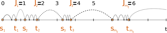
Figure 1. In the figure we have pictured a random set $X$, given as the zero level set of a stochastic process, whose excursions are represented by the semi-arcs (dotted arcs represents excursions between two consecutive visited blocks). The coarse-grained decomposition of $X$ is given by the first and last points – $\mathtt{s}_{k}(X),\mathtt{t}_{k}(X)$ – inside each visited block $[\boldsymbol{\mathtt{J}}_{k}-1(X),\boldsymbol{\mathtt{J}}_{k}(X))$, marked by a big dot in the figure. By construction, between visited blocks there are no points of $X$; all of its points are contained in the set $\cup_{k\in\mathbb{N}}\Big{[}\mathtt{s}_{k}(X),\mathtt{t}_{k}(X)\Big{]}$.

Remark 5.2.

For every $t\in\mathbb{N}$, one has the convergence in distribution

$$\big{(}{\mathtt{m}}_{t}^{(N)},({\mathtt{s}}^{(N)}_{k},{\mathtt{t}}^{(N)}_{k})_{1\leq k\leq{\mathtt{m}}_{t}^{(N)}}\big{)}\xrightarrow[N\to\infty]{d}\big{(}\boldsymbol{\mathtt{m}}_{t},(\boldsymbol{\mathtt{s}}_{k},\boldsymbol{\mathtt{t}}_{k})_{1\leq k\leq\boldsymbol{\mathtt{m}}_{t}}\big{)}\,,$$ (5.9)

thanks to the convergence in distribution of $(\mathtt{g}_{s}(\tau/N),\mathtt{d}_{s}(\tau/N))_{s\in\mathbb{N}}$ toward $(\mathtt{g}_{s}(\boldsymbol{\tau}^{\alpha}),\mathtt{d}_{s}(\boldsymbol{\tau}^{\alpha}))_{s\in\mathbb{N}}$.

Using (5.3) and the regenerative property, one can write explicitly the joint density of $\boldsymbol{\mathtt{J}}_{k},\boldsymbol{\mathtt{s}}_{k},\boldsymbol{\mathtt{t}}_{k}$. This yields the following estimates of independent interest, proved in Appendix A.1.

Lemma 5.3.

For any $\alpha\in(0,1)$ there are constants $A_{\alpha},B_{\alpha}\in(0,\infty)$ such that for all $\gamma\geq 0$

$$\sup_{(x,y)\in[0,1]_{\leq}^{2}}\mathrm{P}_{x}\left(\left.\boldsymbol{\mathtt{t}}_{2}\in[\boldsymbol{\mathtt{J}}_{2}-\gamma,\boldsymbol{\mathtt{J}}_{2}]\,\right|\,\boldsymbol{\mathtt{t}}_{1}=y\right)\leq A_{\alpha}\,\gamma^{1-\alpha}\,,$$ (5.10)

$$\sup_{(x,y)\in[0,1]_{\leq}^{2}}\mathrm{P}_{x}\left(\left.\boldsymbol{\mathtt{t}}_{2}-\boldsymbol{\mathtt{s}}_{2}\leq\gamma\,\right|\,\boldsymbol{\mathtt{t}}_{1}=y\right)\leq B_{\alpha}\,\gamma^{\alpha}\,,$$ (5.11)

where $\mathrm{P}_{x}$ is the law of the $\alpha$-stable regenerative set starting from $x$.

We are ready to express the partition functions $\mathrm{Z}_{\beta_{N},h_{N}}^{\omega}(Nt)$ and $\mathbf{Z}_{\hat{\beta},\hat{h}}^{W}(t)$ in terms of the random sets $\tau/N$ and $\boldsymbol{\tau}^{\alpha}$, through their coarse-grained decompositions. Recall that $\beta_{N},h_{N}$ are linked to $N$ and $\hat{\beta},\hat{h}$ by (2.11). For notational lightness, we denote by $\mathrm{E}$ the expectation with respect to either $\tau/N$ or $\boldsymbol{\tau}^{\alpha}$.

Theorem 5.4 (Coarse-grained Hamiltonians).

For $t\in\mathbb{N}$ we can write the discrete and continuum partition functions as follows:

$$\mathrm{Z}_{\beta_{N},h_{N}}^{\omega}(Nt)=\mathrm{E}\left[e^{\mathrm{H}_{N,t;\hat{\beta},\hat{h}}^{\omega}(\tau/N)}\right]\,,\qquad\mathbf{Z}_{\hat{\beta},\hat{h}}^{W}(t)=\mathrm{E}\left[e^{\mathbf{H}_{t;\hat{\beta},\hat{h}}^{W}(\boldsymbol{\tau}^{\alpha})}\right]\,,$$ (5.12)

where the coarse-grained Hamiltonians $\mathrm{H}(\tau/N)$ and $\mathbf{H}(\boldsymbol{\tau}^{\alpha})$ depend on the random sets $\tau/N$ and $\boldsymbol{\tau}^{\alpha}$ only through their coarse-grained decompositions, and are defined by

$$\mathrm{H}_{N,t;\hat{\beta},\hat{h}}^{\omega}(\tau/N):=\sum_{k=1}^{{\mathtt{m}}_{t}^{(N)}}\log\mathrm{Z}_{\beta_{N},h_{N}}^{\omega,\mathtt{c}}(N{\mathtt{s}}^{(N)}_{k},N{\mathtt{t}}^{(N)}_{k})\,,\qquad\mathbf{H}^{W}_{t;\hat{\beta},\hat{h}}(\boldsymbol{\tau}^{\alpha})=\sum_{k=1}^{\boldsymbol{\mathtt{m}}_{t}}\log\mathbf{Z}_{\hat{\beta},\hat{h}}^{W,\mathtt{c}}(\boldsymbol{\mathtt{s}}_{k},\boldsymbol{\mathtt{t}}_{k})\,.$$ (5.13)

Proof.

Starting from the definition (2.1) of $\mathrm{Z}_{\beta_{N},h_{N}}^{\omega}(Nt)$, we disintegrate according to the random variables ${\mathtt{m}}_{t}^{(N)}$ and $({\mathtt{s}}^{(N)}_{k},{\mathtt{t}}^{(N)}_{k})_{1\leq k\leq{\mathtt{m}}_{t}^{(N)}}$. Recalling (2.24), the renewal property of $\tau$ yields

$$\mathrm{Z}_{\beta_{N},h_{N}}^{\omega}(Nt)= \mathrm{E}\left[\mathrm{Z}_{\beta_{N},h_{N}}^{\omega,\mathtt{c}}(0,N{\mathtt{t}}^{(N)}_{1})\,\mathrm{Z}_{\beta_{N},h_{N}}^{\omega,\mathtt{c}}(N{\mathtt{s}}^{(N)}_{2},N{\mathtt{t}}^{(N)}_{2})\cdots\mathrm{Z}_{\beta_{N},h_{N}}^{\omega,\mathtt{c}}(N{\mathtt{s}}^{(N)}_{{\mathtt{m}}_{t}^{(N)}},N{\mathtt{t}}^{(N)}_{{\mathtt{m}}_{t}^{(N)}})\right]\,,$$ (5.14)

which is precisely the first relation in (5.12), with $\mathrm{H}$ defined as in (5.13).

The second relation in (5.12) can be proved with analogous arguments, by the regenerative property of $\boldsymbol{\tau}^{\alpha}$. Alternatively, one can exploit the convergence in distribution (5.9), that becomes a.s. convergence under a suitable coupling of $\tau/N$ and $\boldsymbol{\tau}^{\alpha}$; since $\mathrm{Z}_{\beta_{N},h_{N}}^{\omega,\mathtt{c}}(Ns,Nt)\to\mathbf{Z}_{\hat{\beta},\hat{h}}^{W,\mathtt{c}}(s,t)$ uniformly for $0\leq s\leq t\leq T$, under a coupling of $\omega$ and $W$ (by Theorem 2.6), letting $N\to\infty$ in (5.14) yields, by dominated convergence, the second relation in (5.12), with $\mathbf{H}$ defined as in (5.13). ∎

The usefulness of the representations in (5.12) is that they express the discrete and continuum partition functions in closely analogous ways, which behave well in the continuum limit $N\to\infty$. To appreciate this fact, note that although the discrete partition function is expressed through an Hamiltonian of the form $\sum_{n=1}^{N}(\beta\omega_{n}-\Lambda(\beta)+h)\mathds{1}_{\{n\in\tau\}}$, cf. (2.1), such a “microscopic” Hamiltonian admits no continuum analogue, because the continuum disordered pinning model studied in [11] is singular with respect to the regenerative set $\boldsymbol{\tau}^{\alpha}$, cf. [11, Theorem 1.5]. The “macroscopic” coarse-grained Hamiltonians in (5.13), on the other hand, will serve our purpose.

5.4. General Strategy

We now describe a general strategy to prove the key relation (2.21) of Theorem 2.4, exploiting the representations in (5.12). We follow the strategy developed for the copolymer model in [9, 10], with some simplifications and strengthenings.

Definition 5.5.

Let $f_{t}(N,\hat{\beta},\hat{h})$ and $g_{t}(N,\hat{\beta},\hat{h})$ be two real functions of $t,N\in\mathbb{N}$, $\hat{\beta}>0$, $\hat{h}\in\mathbb{R}$. We write $f\prec g$ if for all fixed $\hat{\beta},\hat{h},\hat{h}^{\prime}$ with $\hat{h}<\hat{h}^{\prime}$ there exists $N_{0}(\hat{\beta},\hat{h},\hat{h}^{\prime})<\infty$ such that for all $N>N_{0}$

$$\begin{split}&\limsup_{t\to\infty}f_{t}(N,\hat{\beta},\hat{h})\leq\limsup_{t\to\infty}g_{t}(N,\hat{\beta},\hat{h}^{\prime}),\\ &\liminf_{t\to\infty}f_{t}(N,\hat{\beta},\hat{h})\leq\liminf_{t\to\infty}g_{t}(N,\hat{\beta},\hat{h}^{\prime}).\end{split}$$ (5.15)

where the limits are taken along $t\in\mathbb{N}$. If both $f\prec g$ and $g\prec f$ hold, then we write $f\simeq g$.

Keeping in mind (2.5) and (2.14), we define $f^{(1)}$ and $f^{(3)}$ respectively as the continuum and discrete (rescaled) finite-volume free energies, averaged over the disorder:

$$f_{t}^{(1)}(N,\hat{\beta},\hat{h}):=\frac{1}{t}\mathbb{E}\left(\log\mathbf{Z}_{\hat{\beta},\hat{h}}^{W}(t)\right)\,,$$ (5.16)

$$f_{t}^{(3)}(N,\hat{\beta},\hat{h}):=\frac{1}{t}\mathbb{E}\left(\log\mathrm{Z}_{\beta_{N},h_{N}}^{\omega}(Nt)\right)\,.$$ (5.17)

(Note that $f^{(1)}$ does not depend on $N$.) Our goal is to prove that $f^{(3)}\simeq f^{(1)}$, because this yields the key relation (2.21) in Theorem 2.4, and also the existence of the averaged continuum free energy as $t\to\infty$ along $t\in\mathbb{N}$ (thus proving part of Theorem 2.3). Let us start checking these claims.

Lemma 5.6.

Assuming $f^{(3)}\simeq f^{(1)}$, the following limit exists along $t\in\mathbb{N}$ and is finite:

$$\mathbf{F}^{\alpha}(\hat{\beta},\hat{h}):=\lim_{t\to\infty}f_{t}^{(1)}(N,\hat{\beta},\hat{h})=\lim_{t\to\infty}\frac{1}{t}\mathbb{E}\left(\log\mathbf{Z}_{\hat{\beta},\hat{h}}^{W}(t)\right)\,.$$ (5.18)

Proof.

The key point is that $f_{t}^{(3)}$ admits a limit as $t\to\infty$: by (2.5), for all $N\in\mathbb{N}$ we can write

$$\lim_{t\to\infty}f_{t}^{(3)}(N,\hat{\beta},\hat{h})=N\,\mathrm{F}(\beta_{N},h_{N})\,$$ (5.19)

where we agree that limits are taken along $t\in\mathbb{N}$. For every $\epsilon>0$, the relation $f^{(3)}\simeq f^{(1)}$ yields

$$\limsup_{t\to\infty}f_{t}^{(1)}(N,\hat{\beta},\hat{h}-2\epsilon)\leq\lim_{t\to\infty}f_{t}^{(3)}(N,\hat{\beta},\hat{h}-\epsilon)\leq\liminf_{t\to\infty}f_{t}^{(1)}(N,\hat{\beta},\hat{h})\,,$$ (5.20)

for $N\in\mathbb{N}$ large enough (depending on $\hat{\beta},\hat{h}$ and $\epsilon$). Plugging the definition (5.16) of $f_{t}^{(1)}$, which does not depend on $N\in\mathbb{N}$, into this relation, we get

$$\begin{split}\limsup_{t\to\infty}\frac{1}{t}\mathbb{E}\left(\log\mathbf{Z}_{\hat{\beta},\hat{h}-2\epsilon}^{W}(t)\right)\leq\liminf_{t\to\infty}\frac{1}{t}\mathbb{E}\left(\log\mathbf{Z}_{\hat{\beta},\hat{h}}^{W}(t)\right).\end{split}$$ (5.21)

The left hand side of this relation is a convex function of $\epsilon\geq 0$ (being the $\limsup$ of convex functions, by Proposition 2.7) and is finite (it is bounded by $N\,\mathrm{F}(\beta_{N},h_{N})<\infty$, by (5.19) and (5.20)). It follows that it is a continuous function of $\epsilon\geq 0$, so letting $\epsilon\downarrow 0$ completes the proof. ∎

Lemma 5.7.

Assuming $f^{(3)}\simeq f^{(1)}$, relation (2.21) in Theorem 2.4 holds true.

Proof.

We know that $\lim_{t\to\infty}f_{t}^{(1)}(N,\hat{\beta},\hat{h})=\mathbf{F}^{\alpha}(\hat{\beta},\hat{h})$ by Lemma 5.6. Recalling (5.19), relation $f^{(3)}\simeq f^{(1)}$ can be restated as follows: for all $\hat{\beta}>0$, $\hat{h}\in\mathbb{R}$ and $\eta>0$ there exists $N_{0}<\infty$ such that

$$\mathbf{F}^{\alpha}(\hat{\beta},\hat{h}-\eta)\leq N\,\mathrm{F}\left(\hat{\beta}\frac{L(N)}{N^{\alpha-\frac{1}{2}}},\hat{h}\frac{L(N)}{N^{\alpha}}\right)\leq\mathbf{F}^{\alpha}(\hat{\beta},\hat{h}+\eta)\,,\qquad\forall N\geq N_{0}\,.$$

Incidentally, this relation holds also when $N\in[N_{0},\infty)$ is not an integer, because the same holds for relation (5.19). Setting $\epsilon:=\frac{1}{N}$ and $\epsilon_{0}:=\frac{1}{N_{0}}$ yields precisely relation (2.21). ∎

The rest of this section is devoted to proving $f^{(1)}\simeq f^{(3)}$. By (5.16)-(5.17) and (5.12), we can write

$$f_{t}^{(1)}(N,\hat{\beta},\hat{h})=\frac{1}{t}\mathbb{E}\left(\log\mathrm{E}\left[e^{\mathbf{H}_{t;\hat{\beta},\hat{h}}^{W}(\boldsymbol{\tau}^{\alpha})}\right]\right)\,,\qquad f_{t}^{(3)}(N,\hat{\beta},\hat{h})=\frac{1}{t}\mathbb{E}\left(\log\mathrm{E}\left[e^{\mathrm{H}_{N,t;\hat{\beta},\hat{h}}^{\omega}(\tau/N)}\right]\right)\,.$$ (5.22)

Since relation $\simeq$ is transitive, it suffices to prove that

$$f^{(1)}\simeq f^{(2)}\simeq f^{(3)}\,,$$ (5.23)

for a suitable intermediate quantity $f^{(2)}$ which somehow interpolates between $f^{(1)}$ and $f^{(3)}$. We define $f^{(2)}$ replacing the rescaled renewal $\tau/N$ by the regenerative set $\boldsymbol{\tau}^{\alpha}$ in $f^{(3)}$:

$$f_{t}^{(2)}(N,\hat{\beta},\hat{h}):=\frac{1}{t}\mathbb{E}\left(\log\mathrm{E}\left[e^{\mathrm{H}_{N,t;\hat{\beta},\hat{h}}^{\omega}(\boldsymbol{\tau}^{\alpha})}\right]\right)\,.$$ (5.24)

Note that each function $f^{(i)}$, for $i=1,2,3$, is of the form

$$f_{t}^{(i)}(N,\hat{\beta},\hat{h})=\frac{1}{t}\mathbb{E}\left(\log\mathrm{E}\left[e^{\mathrm{H}_{N,t;\hat{\beta},\hat{h}}^{(i)}}\right]\right),$$ (5.25)

for a suitable Hamiltonian $\mathrm{H}_{N,t;\hat{\beta},\hat{h}}^{(i)}$. We recall that $\mathbb{E}$ is expectation with respect to the disorder (either $\omega$ or $W$) while $\mathrm{E}$ is expectation with respect to the random set (either $\tau/N$ or $\boldsymbol{\tau}^{\alpha}$).

The general strategy to to prove $f^{(i)}\prec f^{(j)}$ can be described as follows ($i=1,j=2$ for clarity). For fixed $\hat{\beta},\hat{h},\hat{h}^{\prime}$ with $\hat{h}<\hat{h}^{\prime}$, we couple the two Hamiltonians $\mathrm{H}_{N,t;\hat{\beta},\hat{h}}^{(1)}$ and $\mathrm{H}_{N,t;\hat{\beta},\hat{h}^{\prime}}^{(2)}$ (both with respect to the random set and to the disorder) and we define for $\epsilon\in(0,1)$

$$\Delta_{N,\epsilon}^{(1,2)}(t):=\mathrm{H}_{N,t;\hat{\beta},\hat{h}}^{(1)}-(1-\epsilon)\mathrm{H}_{N,\hat{\beta},\hat{h}^{\prime}}^{(2)}$$ (5.26)

(we omit the dependence of $\Delta_{N,\epsilon}^{(1,2)}(t)$ on $\hat{\beta},\hat{h},\hat{h}^{\prime}$ for short). Hölder’s inequality then gives

$$\mathrm{E}\left(e^{\mathrm{H}_{N,t;\hat{\beta},\hat{h}}^{(1)}}\right)\leq\mathrm{E}\left(e^{\mathrm{H}_{N,t;\hat{\beta},\hat{h}^{\prime}}^{(2)}}\right)^{1-\epsilon}\mathrm{E}\left(e^{\frac{1}{\epsilon}\Delta_{N,\epsilon}^{(1,2)}(t)}\right)^{\epsilon}\,.$$

Denoting by $\lim^{*}_{t\to\infty}$ either $\liminf_{t\to\infty}$ or $\limsup_{t\to\infty}$ (or, for that matter, the limit of any convergent subsequence), recalling (5.25) and applying Jensen’s inequality leads to

$$\lim^{*}_{t\to\infty}f_{t}^{(1)}(N,\hat{\beta},\hat{h})\leq(1-\epsilon)\lim^{*}_{t\to\infty}f_{t}^{(2)}(N,\hat{\beta},\hat{h}^{\prime})+\epsilon\limsup_{t\to\infty}\frac{1}{t}\log\mathrm{E}\mathbb{E}\left(e^{\frac{1}{\epsilon}\Delta^{(1,2)}_{N,\epsilon}(t)}\right)\,.$$

In order to prove $f^{(1)}\prec f^{(2)}$ it then suffices to show the following: for fixed $\hat{\beta},\hat{h},\hat{h}^{\prime}$ with $\hat{h}<\hat{h}^{\prime}$,

$$\begin{split}\exists\epsilon\in(0,1),\ N_{0}\in(0,\infty):\qquad&\limsup_{t\to\infty}\frac{1}{t}\log\mathrm{E}\mathbb{E}\left(e^{\frac{1}{\epsilon}\Delta^{(1,2)}_{N,\epsilon}(t)}\right)\leq 0,\quad\forall N\geq N_{0}\,.\end{split}$$ (5.27)

(Of course, $\epsilon$ and $N_{0}$ will depend on the fixed values of $\hat{\beta},\hat{h},\hat{h}^{\prime}$.)

We will give details only for the proof of $f^{(1)}\prec f^{(2)}\prec f^{(3)}$, because with analogous arguments one proves $f^{(1)}\succ f^{(2)}\succ f^{(3)}$. Before starting, we describe the coupling of the coarse-grained Hamiltonians.

Remark 5.8.

For technical convenience, instead of linearly interpolating the discrete partition functions when $Ns,Nt\not\in\mathbb{N}_{0}$, it will be convenient in §5.7 to consider their piecewise constant extension $\mathrm{Z}_{\beta_{N},h_{N}}^{\omega,\mathtt{c}}(\lfloor Ns\rfloor,\lfloor Nt\rfloor)$. Plainly, relation (4.3) still holds.

5.5. The coupling

The coarse-grained Hamiltonians $\mathrm{H}$ and $\mathbf{H}$, defined in (5.13), are functions of the disorders $\omega$ and $W$ and of the random sets $\tau/N$ and $\boldsymbol{\tau}^{\alpha}$. We now describe how to couple the disorders (the random sets will be coupled through Radon-Nikodym derivatives, cf. §5.7).

Recall that $[a,b)^{2}_{\leq}:=\{(x,y):\ a\leq x\leq y\leq b\}$. For $n\in\mathbb{N}$, we let $\mathtt{Z}^{(n)}_{N}$ and $\boldsymbol{\mathtt{Z}}^{(n)}$ denote the families of discrete and continuum partition functions with endpoints in $[n,n+1)$:

$$\mathtt{Z}^{(n)}_{N}:=\left(\mathrm{Z}_{\beta_{N},h_{N}}^{\omega,\mathtt{c}}(Ns,Nt)\right)_{(s,t)\in[n,n+1)^{2}_{\leq}}\,,\qquad\boldsymbol{\mathtt{Z}}^{(n)}:=\left(\mathbf{Z}_{\hat{\beta},\hat{h}}^{W,\mathtt{c}}(s,t)\right)_{(s,t)\in[n,n+1)^{2}_{\leq}}\,.$$

Note that both $(\mathtt{Z}^{(n)}_{N})_{n\in\mathbb{N}}$ and $(\boldsymbol{\mathtt{Z}}^{(n)})_{n\in\mathbb{N}}$ are i.i.d. sequences. A look at (5.13) reveals that that the coarse-grained Hamiltonian $\mathrm{H}$ depends on the disorder $\omega$ only through $(\mathtt{Z}^{(n)}_{N})_{n\in\mathbb{N}}$, and likewise $\mathbf{H}$ depends on $W$ only through $(\boldsymbol{\mathtt{Z}}^{(n)})_{n\in\mathbb{N}}$. Consequently, to couple $\mathrm{H}$ and $\mathbf{H}$ it suffices to couple $(\mathtt{Z}^{(n)}_{N})_{n\in\mathbb{N}}$ and $(\boldsymbol{\mathtt{Z}}^{(n)})_{n\in\mathbb{N}}$, i.e. to define a law for the joint sequence $\big{(}(\mathtt{Z}^{(n)}_{N},\boldsymbol{\mathtt{Z}}^{(n)})\big{)}_{n\in\mathbb{N}}$. We take this to be i.i.d.: discrete and continuum partition functions are coupled independently in each block $[n,n+1)$.

It remains to define a coupling for $\mathtt{Z}^{(1)}_{N}$ and $\boldsymbol{\mathtt{Z}}^{(1)}$. Throughout the sequel we fix $\hat{\beta}>0$ and $\hat{h},\hat{h}^{\prime}\in\mathbb{R}$ with $\hat{h}<\hat{h}^{\prime}$. We can then use the coupling provided by Theorem 2.6, which ensures that relation (4.3) holds $\mathbb{P}(\mathrm{d}\omega,\mathrm{d}W)$-a.s., with $T=1$ and $M=\max\{|\hat{h}|,|\hat{h}^{\prime}|\}$.

5.6. First step: $f^{(1)}\prec f^{(2)}$

Our goal is to prove (5.27). Recalling (5.26), (5.22) and (5.24), as well as (5.13), for fixed $\hat{\beta},\hat{h},\hat{h}^{\prime}$ with $\hat{h}<\hat{h}^{\prime}$ we can write

$$\Delta_{N,\epsilon}^{(1,2)}(t)=\mathbf{H}_{t;\hat{\beta},\hat{h}}^{W}(\boldsymbol{\tau}^{\alpha})-(1-\epsilon)\mathrm{H}_{N,t;\hat{\beta},\hat{h}^{\prime}}^{W}(\boldsymbol{\tau}^{\alpha})=\sum_{k=1}^{\boldsymbol{\mathtt{m}}_{t}}\log\frac{\mathbf{Z}_{\hat{\beta},\hat{h}}^{W,\mathtt{c}}(\boldsymbol{\mathtt{s}}_{k},\boldsymbol{\mathtt{t}}_{k})}{\mathrm{Z}_{\beta_{N},h_{N}^{\prime}}^{\omega,\mathtt{c}}(N\boldsymbol{\mathtt{s}}_{k},N\boldsymbol{\mathtt{t}}_{k})^{1-\epsilon}},$$ (5.28)

where we set $h^{\prime}_{N}=\hat{h}^{\prime}L(N)/N^{\alpha}$ for short, cf. (2.11). Consequently

$$\mathrm{E}\mathbb{E}\left(e^{\frac{1}{\epsilon}\Delta_{N,\epsilon}^{(1,2)}(t)}\right)=\mathrm{E}\left[\prod_{k=1}^{\boldsymbol{\mathtt{m}}_{t}}f_{N,\epsilon}(\boldsymbol{\mathtt{s}}_{k},\boldsymbol{\mathtt{t}}_{k})\right]\,,\quad\ \ \text{where}\quad f_{N,\epsilon}(s,t):=\mathbb{E}\left[\left(\frac{\mathbf{Z}_{\hat{\beta},\hat{h}}^{W,\mathtt{c}}(s,t)}{\mathrm{Z}_{\beta_{N},h_{N}^{\prime}}^{\omega,\mathtt{c}}(Ns,Nt)^{1-\epsilon}}\right)^{\frac{1}{\epsilon}}\right]\,,$$ (5.29)

because discrete and continuum partition functions are coupled independently in each block $[n,n+1)$, cf. §5.5, hence the $\mathbb{E}$-expectation factorizes. (Of course, $f_{N,\epsilon}(s,t)$ also depends on $\hat{\beta},\hat{h},\hat{h}^{\prime}$.)

Let us denote by $\mathcal{F}_{M}=\sigma\left((\boldsymbol{\mathtt{s}}_{i},\boldsymbol{\mathtt{t}}_{i}):i\leq M\right)$ the filtration generated by the first $M$ visited blocks. By the regenerative property, the regenerative set $\boldsymbol{\tau}^{\alpha}$ starts afresh at the stopping time $\boldsymbol{\mathtt{s}}_{k-1}$, hence

$$\mathrm{E}\big{[}f_{N,\epsilon}(\boldsymbol{\mathtt{s}}_{k},\boldsymbol{\mathtt{t}}_{k})\,|\,\mathcal{F}_{k-1}\big{]}=\mathrm{E}\big{[}f_{N,\epsilon}(\boldsymbol{\mathtt{s}}_{k},\boldsymbol{\mathtt{t}}_{k})\,|\,\boldsymbol{\mathtt{s}}_{k-1},\boldsymbol{\mathtt{t}}_{k-1}\big{]}\,,$$ (5.30)

where we agree that $\mathrm{E}[\,\cdot\,|\,\boldsymbol{\mathtt{s}}_{0},\boldsymbol{\mathtt{t}}_{0}]:=\mathrm{E}[\,\cdot\,]$. Defining the constant

$$\Lambda_{N,\epsilon}:=\sup_{k,\boldsymbol{\mathtt{s}}_{k-1},\boldsymbol{\mathtt{t}}_{k-1}}\mathrm{E}\big{[}f_{N,\epsilon}(\boldsymbol{\mathtt{s}}_{k},\boldsymbol{\mathtt{t}}_{k})\,|\,\boldsymbol{\mathtt{s}}_{k-1},\boldsymbol{\mathtt{t}}_{k-1}\big{]}\,,$$ (5.31)

we have $\mathrm{E}\big{[}f_{N,\epsilon}(\boldsymbol{\mathtt{s}}_{k},\boldsymbol{\mathtt{t}}_{k})\,|\,\mathcal{F}_{k-1}\big{]}\leq\Lambda_{N,\epsilon}$, hence $\mathrm{E}\left[\prod_{k=1}^{M}f_{N,\epsilon}(\boldsymbol{\mathtt{s}}_{k},\boldsymbol{\mathtt{t}}_{k})\right]\leq(\Lambda_{N,\epsilon})^{M}$ for every $M\in\mathbb{N}$, hence

$$\mathrm{E}\mathbb{E}\left(e^{\frac{1}{\epsilon}\Delta_{N,\epsilon}^{(1,2)}(t)}\right)=\mathrm{E}\left[\prod_{k=1}^{\boldsymbol{\mathtt{m}}_{t}}f_{N,\epsilon}(\boldsymbol{\mathtt{s}}_{k},\boldsymbol{\mathtt{t}}_{k})\right]\leq\sum_{M=1}^{\infty}\mathrm{E}\left[\prod_{k=1}^{M}f_{N,\epsilon}(\boldsymbol{\mathtt{s}}_{k},\boldsymbol{\mathtt{t}}_{k})\right]\leq\sum_{M=1}^{\infty}(\Lambda_{N,\epsilon})^{M}=\frac{\Lambda_{N,\epsilon}}{1-\Lambda_{N,\epsilon}}<\infty\,,$$ (5.32)

provided $\Lambda_{N,\epsilon}<1$. The next Lemma shows that this is indeed the case, if $\epsilon>0$ is small enough and $N>N_{0}(\epsilon)$. This completes the proof of (5.27), hence of $f^{(1)}\prec f^{(2)}$.

Lemma 5.9.

The following relation holds for $\Lambda_{N,\epsilon}$ defined in (5.31), with $f_{N,\epsilon}$ defined in (5.29):

$$\limsup_{\epsilon\to 0}\,\limsup_{N\to\infty}\,\Lambda_{N,\epsilon}=0\,.$$ (5.33)

The proof of Lemma 5.9 is deferred to the Appendix A.2. The key idea is that, for fixed $s<t$, the function $f_{N,\epsilon}(s,t)$ in (5.29) is small when $\epsilon>0$ small and $N$ large, because the discrete partition function in the denominator is close to the continuum one appearing in the numerator, but with $\hat{h}^{\prime}>\hat{h}$ (recall that the continuum partition function is strictly increasing in $\hat{h}$, by Proposition 2.7). To prove that $\Lambda_{N,\epsilon}$ in (5.31) is small, we replace $s,t$ by the random points $\boldsymbol{\mathtt{s}}_{k},\boldsymbol{\mathtt{t}}_{k}$, showing that they cannot be too close to each other, conditionally on (and uniformly over) $\boldsymbol{\mathtt{s}}_{k-1},\boldsymbol{\mathtt{t}}_{k-1}$.

5.7. Second Step: $f^{(2)}\prec f^{(3)}$

Recalling (5.22) and (5.12)-(5.13), we can write $f^{(3)}$ as follows:

$$f_{t}^{(3)}(N,\hat{\beta},\hat{h})=\frac{1}{t}\mathbb{E}\left(\log\mathrm{E}\left[\prod_{k=1}^{{\mathtt{m}}_{t}^{(N)}}\mathrm{Z}_{\beta_{N},h_{N}}^{\omega,\mathtt{c}}(N{\mathtt{s}}^{(N)}_{k},N{\mathtt{t}}^{(N)}_{k})\right]\right)\,.$$ (5.34)

Note that $f^{(2)}$, defined in (5.24), enjoys the same representation (5.34), with ${\mathtt{m}}_{t}^{(N)}$ and ${\mathtt{s}}^{(N)}_{k},{\mathtt{t}}^{(N)}_{k}$ replaced respectively by their continuum counterparts $\boldsymbol{\mathtt{m}}_{t}$ and $\boldsymbol{\mathtt{s}}_{k},\boldsymbol{\mathtt{t}}_{k}$. Since we extend the discrete partition function in a piecewise constant fashion $\mathrm{Z}_{\beta_{N},h_{N}}^{\omega,\mathtt{c}}(\lfloor Ns\rfloor,\lfloor Nt\rfloor)$, cf. Remark 5.8, we can replace $\boldsymbol{\mathtt{s}}_{k},\boldsymbol{\mathtt{t}}_{k}$ by their left neighbors $\boldsymbol{\mathtt{s}}^{(N)}_{k},\boldsymbol{\mathtt{t}}^{(N)}_{k}$ on the lattice $\frac{1}{N}\mathbb{N}_{0}$, i.e.

$$\boldsymbol{\mathtt{s}}^{(N)}_{k}:=\frac{\lfloor N\boldsymbol{\mathtt{s}}_{k}\rfloor}{N}\,,\qquad\boldsymbol{\mathtt{t}}^{(N)}_{k}:=\frac{\lfloor N\boldsymbol{\mathtt{t}}_{k}\rfloor}{N}\,,$$ (5.35)

getting to the following representation for $f_{t}^{(2)}$:

$$f_{t}^{(2)}(N,\hat{\beta},\hat{h})=\frac{1}{t}\mathbb{E}\left(\log\mathrm{E}\left[\prod_{k=1}^{\boldsymbol{\mathtt{m}}_{t}}\mathrm{Z}_{\beta_{N},h_{N}}^{\omega,\mathtt{c}}(N\boldsymbol{\mathtt{s}}^{(N)}_{k},N\boldsymbol{\mathtt{t}}^{(N)}_{k})\right]\right)\,.$$ (5.36)

The random vectors $(\boldsymbol{\mathtt{m}}_{t},(\boldsymbol{\mathtt{s}}^{(N)}_{k},\boldsymbol{\mathtt{t}}^{(N)}_{k})_{1\leq k\leq\boldsymbol{\mathtt{m}}_{t}^{(N)}})$ and $({\mathtt{m}}_{t}^{(N)},({\mathtt{s}}^{(N)}_{k},{\mathtt{t}}^{(N)}_{k})_{1\leq k\leq{\mathtt{m}}_{t}^{(N)}})$ are mutually absolutely continuous. Let us denote by $\mathrm{R}_{t}$ the Radon-Nikodym derivative

$$\mathrm{R}_{t}\left(M,(x_{k},y_{k})_{k=1}^{M}\right)=\frac{\mathrm{P}\left({\mathtt{m}}_{t}^{(N)}=M,({\mathtt{s}}^{(N)}_{k},{\mathtt{t}}^{(N)}_{k})_{k=1}^{m}=(x_{k},y_{k})_{k=1}^{M}\right)}{\mathrm{P}\left(\boldsymbol{\mathtt{m}}_{t}=M,(\boldsymbol{\mathtt{s}}^{(N)}_{k},\boldsymbol{\mathtt{t}}^{(N)}_{k})_{k=1}^{M}=(x_{k},y_{k})_{k=1}^{M}\right)}\,,$$ (5.37)

for $M\in\mathbb{N}$ and $x_{k},y_{k}\in\frac{1}{N}\mathbb{N}_{0}$ (note that necessarily $x_{1}=0$). We can then rewrite (5.34) as follows:

$$f_{t}^{(3)}(N,\hat{\beta},\hat{h})=\frac{1}{t}\mathbb{E}\left(\log\mathrm{E}\left[\prod_{k=1}^{\boldsymbol{\mathtt{m}}_{t}}\left(\mathrm{Z}_{\beta_{N},h_{N}}^{\omega,\mathtt{c}}(N\boldsymbol{\mathtt{s}}^{(N)}_{k},N\boldsymbol{\mathtt{t}}^{(N)}_{k})\right)\cdot\mathrm{R}_{t}\left(\boldsymbol{\mathtt{m}}_{t},(\boldsymbol{\mathtt{s}}^{(N)}_{k},\boldsymbol{\mathtt{t}}^{(N)}_{k})_{k=1}^{\boldsymbol{\mathtt{m}}_{t}}\right)\right]\right)\,,$$ (5.38)

which is identical to (5.36), apart from the Radon-Nikodym derivative $\mathrm{R}_{t}$.

Relations (5.36) and (5.38) are useful because $f_{t}^{(2)}$ and $f_{t}^{(3)}$ are averaged with respect to the same random set $\boldsymbol{\tau}^{\alpha}$ (through its coarse-grained decomposition $\boldsymbol{\mathtt{m}}_{t}$ and $\boldsymbol{\mathtt{s}}^{(N)}_{k},\boldsymbol{\mathtt{t}}^{(N)}_{k}$). This allows to apply the general strategy of §5.4. Defining $\Delta_{N,\epsilon}=\Delta^{(2,3)}_{N,\epsilon}$ as in (5.26), we can write by (5.36)-(5.38)

$$\begin{split}\mathrm{E}\mathbb{E}\left(e^{\frac{1}{\epsilon}\Delta_{N,\epsilon}(t)}\right)=\mathrm{E}\left[\left\{\prod_{k=1}^{\boldsymbol{\mathtt{m}}_{t}}\mathbb{E}\left[\left(\frac{\mathrm{Z}_{\beta_{N},h_{N}}^{\omega,\mathtt{c}}(N\boldsymbol{\mathtt{s}}^{(N)}_{k},N\boldsymbol{\mathtt{t}}^{(N)}_{k})}{\mathrm{Z}_{\beta_{N},h_{N}^{\prime}}^{\omega,\mathtt{c}}(N\boldsymbol{\mathtt{s}}^{(N)}_{k},N\boldsymbol{\mathtt{t}}^{(N)}_{k})^{1-\epsilon}}\right)^{\frac{1}{\epsilon}}\right]\,\right\}\,\mathrm{R}_{t}\left(\boldsymbol{\mathtt{m}}_{t},(\boldsymbol{\mathtt{s}}^{(N)}_{k},\boldsymbol{\mathtt{t}}^{(N)}_{k})_{k=1}^{\boldsymbol{\mathtt{m}}_{t}}\right)^{\frac{1}{\epsilon}}\right],\end{split}$$ (5.39)

and our goal is to prove (5.27) with $\Delta^{(1,2)}_{N,\epsilon}$ replaced by $\Delta_{N,\epsilon}$: explicitly, for fixed $\hat{\beta},\hat{h},\hat{h}^{\prime}$ with $\hat{h}<\hat{h}^{\prime}$,

$$\begin{split}\exists\epsilon\in(0,1),\ N_{0}\in(0,\infty):\qquad&\limsup_{t\to\infty}\frac{1}{t}\log\mathrm{E}\mathbb{E}\left(e^{\frac{1}{\epsilon}\Delta_{N,\epsilon}(t)}\right)\leq 0,\quad\forall N\geq N_{0}\,.\end{split}$$ (5.40)

In order to simplify (5.39), in analogy with (5.29), we define

$$g_{N,\epsilon}(s,t):=\mathbb{E}\left[\left(\frac{\mathrm{Z}_{\beta_{N},h_{N}}^{\omega,\mathtt{c}}(Ns,Nt)}{\mathrm{Z}_{\beta_{N},h_{N}^{\prime}}^{\omega,\mathtt{c}}(Ns,Nt)^{1-\epsilon}}\right)^{\frac{1}{\epsilon}}\right]\,.$$ (5.41)

The Radon-Nikodym derivative $\mathrm{R}_{t}$ in (5.37) does not factorize exactly, but an approximate factorization holds: as we show in section A.3 (cf. Lemma A.1), for suitable functions $r_{N}$ and $\tilde{r}_{N}$

$$\mathrm{R}_{t}\left(M,(x_{k},y_{k})_{k=1}^{M}\right)\leq\left\{\prod_{\ell=1}^{M}r_{N}(y_{\ell-1},x_{\ell},y_{\ell})\right\}\tilde{r}_{N}(y_{M},t)\,,$$ (5.42)

where we set $y_{0}:=0$ (also note that $x_{1}=0$). Looking back at (5.39), we can write

$$\begin{split}\mathrm{E}\mathbb{E}\left(e^{\frac{1}{\epsilon}\Delta_{N,\epsilon}(t)}\right)\leq\mathrm{E}\left[\left\{\prod_{k=1}^{\boldsymbol{\mathtt{m}}_{t}}g_{N,\epsilon}\left(\boldsymbol{\mathtt{s}}^{(N)}_{k},\boldsymbol{\mathtt{t}}^{(N)}_{k}\right)\,r_{N}\left(\boldsymbol{\mathtt{t}}^{(N)}_{k-1},\boldsymbol{\mathtt{s}}^{(N)}_{k},\boldsymbol{\mathtt{t}}^{(N)}_{k}\right)^{\frac{1}{\epsilon}}\right\}\,\tilde{r}_{N}\left(\boldsymbol{\mathtt{t}}^{(N)}_{\boldsymbol{\mathtt{m}}_{t}},t\right)^{\frac{1}{\epsilon}}\right]\,.\end{split}$$ (5.43)

Let us now explain the strategy. We can easily get rid of the last term $\tilde{r}_{N}$ by Cauchy-Schwarz, so we focus on the product appearing in brackets. The goal would be to prove that (5.40) holds by bounding (5.43) through a geometric series, as in (5.32). This could be obtained, in analogy with (5.30)-(5.31), by showing that for $\epsilon$ small and $N$ large the conditional expectation

$$\mathrm{E}\left[\left.g_{N,\epsilon}(\boldsymbol{\mathtt{s}}^{(N)}_{k},\boldsymbol{\mathtt{t}}^{(N)}_{k})\,r_{N}(\boldsymbol{\mathtt{t}}^{(N)}_{k-1},\boldsymbol{\mathtt{s}}^{(N)}_{k},\boldsymbol{\mathtt{t}}^{(N)}_{k})^{\frac{1}{\epsilon}}\right|\mathcal{F}_{k-1}\right]=\mathrm{E}\left[\left.g_{N,\epsilon}(\boldsymbol{\mathtt{s}}^{(N)}_{k},\boldsymbol{\mathtt{t}}^{(N)}_{k})\,r_{N}(\boldsymbol{\mathtt{t}}^{(N)}_{k-1},\boldsymbol{\mathtt{s}}^{(N)}_{k},\boldsymbol{\mathtt{t}}^{(N)}_{k})^{\frac{1}{\epsilon}}\right|\boldsymbol{\mathtt{s}}_{k-1},\boldsymbol{\mathtt{t}}_{k-1}\right]$$

is smaller than $1$, uniformly in $\boldsymbol{\mathtt{s}}_{k-1},\boldsymbol{\mathtt{t}}_{k-1}$. Unfortunately this fails, because the Radon-Nikodym term $r_{N}$ is not small when $\boldsymbol{\mathtt{t}}_{k-1}$ is close to the right end of the block to which it belongs, i.e. to $\boldsymbol{\mathtt{J}}_{k-1}$.

To overcome this difficulty, we distinguish the two events $\{\boldsymbol{\mathtt{t}}_{k-1}\leq\boldsymbol{\mathtt{J}}_{k-1}-\gamma\}$ and $\{\boldsymbol{\mathtt{t}}_{k-1}>\boldsymbol{\mathtt{J}}_{k-1}-\gamma\}$, for $\gamma>0$ that will be chosen small enough. The needed estimates on the functions $g_{N,\epsilon}$, $r_{N}$ and $\tilde{r}_{N}$ are summarized in the next Lemma, proved in Appendix A.3. Let us define for $p\geq 1$ the constant

$$\begin{split}\Lambda_{N,\epsilon,p}:=\sup_{k,\boldsymbol{\mathtt{s}}_{k-1},\boldsymbol{\mathtt{t}}_{k-1}}\mathrm{E}\left(\left.g_{N,\epsilon}(\boldsymbol{\mathtt{s}}_{k},\,\boldsymbol{\mathtt{t}}_{k})^{p}\,\right|\,\boldsymbol{\mathtt{s}}_{k-1},\boldsymbol{\mathtt{t}}_{k-1}\right)\,,\end{split}$$ (5.44)

where we recall that $g_{N,\epsilon}(s,t)$ is defined in (5.41), and we agree that $\mathrm{E}[\,\cdot\,|\,\boldsymbol{\mathtt{s}}_{0},\boldsymbol{\mathtt{t}}_{0}]:=\mathrm{E}[\,\cdot\,]$.

Lemma 5.10.

Let us fix $\hat{\beta}\in\mathbb{R}$ and $\hat{h},\hat{h}^{\prime}\in\mathbb{R}$ with $\hat{h}<\hat{h}^{\prime}$.

• For all $p\geq 1$

  $$\limsup_{\epsilon\to 0}\,\limsup_{N\to\infty}\,\Lambda_{N,\epsilon,p}=0\,.$$ (5.45)

• For all $\epsilon\in(0,1)$, $p\geq 1$ there is $C_{\epsilon,\,p}<\infty$ such that for all $N\in\mathbb{N}$

  $$\forall k\geq 2:\quad\mathrm{E}\left[\left.r_{N}\left(\boldsymbol{\mathtt{t}}^{(N)}_{k-1},\,\boldsymbol{\mathtt{s}}^{(N)}_{k},\,\boldsymbol{\mathtt{t}}^{(N)}_{k}\right)^{\frac{p}{\epsilon}}\,\right|\,\boldsymbol{\mathtt{s}}_{k-1}\,\boldsymbol{\mathtt{t}}_{k-1}\right]\leq C_{\epsilon,p}\,,$$ (5.46)

  $$\mathrm{E}\left[\tilde{r}_{N}\left(\boldsymbol{\mathtt{t}}^{(N)}_{\boldsymbol{\mathtt{m}}_{t}},t\right)^{\frac{p}{\epsilon}}\right]\,\leq C_{\epsilon,p}\,.$$ (5.47)

• For all $\epsilon\in(0,1)$, $p\geq 1$, $\gamma\in(0,1)$ there is $\tilde{N}_{0}=\tilde{N}_{0}(\epsilon,\,p,\,\gamma)<\infty$ such that for $N\geq\tilde{N}_{0}$

  $$\forall k\geq 2:\quad\mathrm{E}\left[\left.r_{N}\left(\boldsymbol{\mathtt{t}}^{(N)}_{k-1},\,\boldsymbol{\mathtt{s}}^{(N)}_{k},\,\boldsymbol{\mathtt{t}}^{(N)}_{k}\right)^{\frac{p}{\epsilon}}\,\right|\,\boldsymbol{\mathtt{s}}_{k-1}\,\boldsymbol{\mathtt{t}}_{k-1}\right]\leq 2\quad\text{on the event}\ \{\boldsymbol{\mathtt{t}}_{k-1}\leq\boldsymbol{\mathtt{J}}_{k-1}-\gamma\}\,,$$ (5.48)

  $$\mathrm{E}\left[r_{N}\left(0,\,0,\,\boldsymbol{\mathtt{t}}^{(N)}_{1}\right)^{\frac{p}{\epsilon}}\,\right]\,\leq 2\,.$$ (5.49)

We are ready to estimate (5.43), with the goal of proving (5.40). Let us define

$$\Phi_{k,N}^{(\epsilon)}:=g_{N,\epsilon}\left(\boldsymbol{\mathtt{s}}^{(N)}_{k},\,\boldsymbol{\mathtt{t}}^{(N)}_{k}\right)^{2}\,r_{N}\left(\boldsymbol{\mathtt{t}}^{(N)}_{k-1},\,\boldsymbol{\mathtt{s}}^{(N)}_{k},\,\boldsymbol{\mathtt{t}}^{(N)}_{k}\right)^{\frac{2}{\epsilon}},$$ (5.50)

with the convention that $\boldsymbol{\mathtt{t}}^{(N)}_{0}:=0$ (note that also $\boldsymbol{\mathtt{s}}^{(N)}_{1}=0$). Then, by (5.47) and Cauchy-Schwarz,

$$\mathrm{E}\mathbb{E}\left(e^{\frac{1}{\epsilon}\Delta_{N,\epsilon}(t)}\right)\leq C_{\epsilon,2}\,\mathrm{E}\left[\prod\limits_{k=1}^{\boldsymbol{\mathtt{m}}_{t}}\Phi_{k,N}^{(\epsilon)}\right]\leq C_{\epsilon,2}\,\sum\limits_{M=1}^{\infty}\mathrm{E}\left[\prod\limits_{k=1}^{M}\Phi_{k,N}^{(\epsilon)}\right]\,.$$

We are going to show that

$$\exists\epsilon\in(0,1),\ N_{0}\in(0,\infty):\qquad\mathrm{E}\left[\prod\limits_{k=1}^{M}\Phi_{k,N}^{(\epsilon)}\right]\leq\frac{1}{2^{M}}\quad\forall M\in\mathbb{N},\ N\geq N_{0}\,,$$ (5.51)

which yields the upper bound $\mathrm{E}\mathbb{E}(e^{\frac{1}{\epsilon}\Delta_{N,\epsilon}(t)})\leq C_{\epsilon,2}$, completing the proof of (5.40).

In the next Lemma, that will be proved in a moment, we single out some properties of $\Phi_{k,N}^{(\epsilon)}$, that are direct consequence of Lemma 5.10.

Lemma 5.11.

One can choose $\epsilon\in(0,1)$, $c\in(1,\infty)$, $\gamma\in(0,1)$ and $N_{0}<\infty$ such that for $N\geq N_{0}$

$$\mathrm{E}\left[\Phi_{1,N}^{(\epsilon)}\right]\leq\,\frac{1}{4}\,;\qquad\ \forall k\geq 2:\ \ \ \mathrm{E}\left[\left.\Phi_{k,N}^{(\epsilon)}\,\right|\,\boldsymbol{\mathtt{s}}_{k-1},\,\boldsymbol{\mathtt{t}}_{k-1}\right]\leq\begin{cases}c&\text{always}\\ \frac{1}{4}&\text{on}\ \{\boldsymbol{\mathtt{t}}_{k-1}\leq\boldsymbol{\mathtt{J}}_{k-1}-\gamma\}\end{cases}\,,$$ (5.52)

and moreover

$$\mathrm{E}\left[\Phi_{1,N}^{(\epsilon)}\mathds{1}_{\{\boldsymbol{\mathtt{t}}_{1}>1-\gamma\}}\right]\leq\frac{1}{8c}\,;\qquad\forall k\geq 2:\ \ \ \mathrm{E}\left[\left.\Phi_{k,N}^{(\epsilon)}\mathds{1}_{\{\boldsymbol{\mathtt{t}}_{k}>\boldsymbol{\mathtt{J}}_{k}-\gamma\}}\,\right|\,\boldsymbol{\mathtt{s}}_{k-1},\,\boldsymbol{\mathtt{t}}_{k-1}\right]\leq\frac{1}{8c}\,.$$ (5.53)

Let us now deduce (5.51). We fix $\epsilon$, $c$, $\gamma$ and $N_{0}$ as in Lemma 5.11. Setting for compactness

$$D_{M,N}:=\prod\limits_{k=1}^{M}\Phi_{k,N}^{(\epsilon)}\,,$$

we show the following strengthened version of (5.51):

$$\mathrm{E}\left[D_{M,N}\right]\leq\,\frac{1}{2^{M}}\,,\qquad\mathrm{E}\left[D_{M,N}\mathds{1}_{\{\boldsymbol{\mathtt{t}}_{M}>\boldsymbol{\mathtt{J}}_{M}-\gamma\}}\right]\leq\,\frac{1}{c2^{M+2}}\,,\qquad\forall M\in\mathbb{N}\,,\ N\geq N_{0}\,.$$ (5.54)

We proceed by induction on $M\in\mathbb{N}$. The case $M=1$ holds by the first relations in (5.52), (5.53). For the inductive step, we fix $M\geq 2$ and we assume that (5.54) holds for $M-1$, then

$$\mathrm{E}\left[D_{M,N}\right] =\mathrm{E}\left[D_{M-1,N}\,\mathrm{E}\left(\left.\Phi_{M,N}^{(\epsilon)}\,\right|\,\mathcal{F}_{M-1}\right)\right]=\mathrm{E}\left[D_{M-1,N}\,\mathrm{E}\left(\left.\Phi_{M,N}^{(\epsilon)}\,\right|\,\boldsymbol{\mathtt{s}}_{M-1},\,\boldsymbol{\mathtt{t}}_{M-1}\right)\right]$$

$$=\mathrm{E}\left[D_{M-1,N}\,\mathrm{E}\left(\left.\Phi_{M,N}^{(\epsilon)}\,\right|\,\boldsymbol{\mathtt{s}}_{M-1},\,\boldsymbol{\mathtt{t}}_{M-1}\right)\mathds{1}_{\{\boldsymbol{\mathtt{t}}_{M-1}>\boldsymbol{\mathtt{J}}_{M-1}-\gamma\}}\right]$$

$$\qquad+\mathrm{E}\left[D_{M-1,N}\,\mathrm{E}\left(\left.\Phi_{M,N}^{(\epsilon)}\,\right|\,\boldsymbol{\mathtt{s}}_{M-1},\,\boldsymbol{\mathtt{t}}_{M-1}\right)\mathds{1}_{\{\boldsymbol{\mathtt{t}}_{M-1}\leq\boldsymbol{\mathtt{J}}_{M-1}-\gamma\}}\right]$$

$$\leq c\,\mathrm{E}\left[D_{M-1,N}\mathds{1}_{\{\boldsymbol{\mathtt{t}}_{M-1}>\boldsymbol{\mathtt{J}}_{M-1}-\gamma\}}\right]\,+\,\frac{1}{4}\,\mathrm{E}\left[D_{M-1,N}\right]\leq c\,\frac{1}{c2^{M+1}}+\frac{1}{4}\frac{1}{2^{M-1}}\leq\frac{1}{2^{M}}\,,$$

where in the last line we have applied (5.52) and the induction step. Similarly, applying the second relation in (5.53) and the induction step,

$$\mathrm{E}\left[{D_{M,N}}\mathds{1}_{\{\boldsymbol{\mathtt{t}}_{M}>\boldsymbol{\mathtt{J}}_{M}-\gamma\}}\right]=\mathrm{E}\left[\left.D_{M-1,N}\mathrm{E}\left({\Phi_{M,N}^{(\epsilon)}}\mathds{1}_{\{\boldsymbol{\mathtt{t}}_{M}>\boldsymbol{\mathtt{J}}_{M}-\gamma\}}\,\right|\,\boldsymbol{\mathtt{s}}_{M-1},\,\boldsymbol{\mathtt{t}}_{M-1}\right)\right]\leq\frac{1}{8c}\mathrm{E}\left[D_{M-1,N}\right]\leq\frac{1}{c2^{M+2}}.$$

This completes the proof of (5.54), hence of (5.51), hence of $f^{(2)}\prec f^{(3)}$.

Proof of Lemma 5.11.

We fix $\epsilon>0$ such that, by relation (5.45), for some $\hat{N}_{0}<\infty$ one has

$$\Lambda_{N,\epsilon,4p}\leq\frac{1}{32}\,,\quad\forall N\geq\hat{N}_{0},\quad\text{for both }p=1\text{ and }p=2\,.$$ (5.55)

Given the parameter $\gamma\in(0,1)$, to be fixed later, we are going to apply relations (5.48)-(5.49), that hold for $N\geq\tilde{N}_{0}(\gamma)$ and for $p\in\{1,2\}$ (we stress that $\epsilon$ has been fixed). Defining $N_{0}:=\max\{\tilde{N}_{0}(\gamma),\hat{N}_{0}\}$, whose value will be fixed once $\gamma$ is fixed, henceforth we assume that $N\geq N_{0}$.

Recalling (5.50) and (5.44), for $k\geq 2$ and $p\in\{1,2\}$ one has, by Cauchy-Schwarz,

$$\begin{split}\mathrm{E}\left[\left.\left(\Phi_{k,N}^{(\epsilon)}\right)^{p}\,\right|\,\boldsymbol{\mathtt{s}}_{k-1},\,\boldsymbol{\mathtt{t}}_{k-1}\right]^{2}&\leq\mathrm{E}\left[\left.g_{N,\epsilon}\left(\boldsymbol{\mathtt{s}}^{(N)}_{k},\,\boldsymbol{\mathtt{t}}^{(N)}_{k}\right)^{4p}\,\right|\,\boldsymbol{\mathtt{s}}_{k-1},\,\boldsymbol{\mathtt{t}}_{k-1}\right]\cdot\\ &\qquad\quad\cdot\mathrm{E}\left[\left.r_{N}\left(\boldsymbol{\mathtt{t}}^{(N)}_{k-1},\,\boldsymbol{\mathtt{s}}^{(N)}_{k},\,\boldsymbol{\mathtt{t}}^{(N)}_{k}\right)^{\frac{4p}{\epsilon}}\,\right|\,\boldsymbol{\mathtt{s}}_{k-1},\,\boldsymbol{\mathtt{t}}_{k-1}\right]\\ &\leq\Lambda_{N,\epsilon,4p}\cdot\mathrm{E}\left[\left.r_{N}\left(\boldsymbol{\mathtt{t}}^{(N)}_{k-1},\,\boldsymbol{\mathtt{s}}^{(N)}_{k},\,\boldsymbol{\mathtt{t}}^{(N)}_{k}\right)^{\frac{4p}{\epsilon}}\,\right|\,\boldsymbol{\mathtt{s}}_{k-1},\,\boldsymbol{\mathtt{t}}_{k-1}\right]\\ &\leq\begin{cases}\frac{1}{32}\cdot C_{\epsilon,4p}&\text{always}\\ \frac{1}{32}\cdot 2=\frac{1}{4^{2}}&\text{on }\ \{\boldsymbol{\mathtt{t}}_{k-1}\leq\boldsymbol{\mathtt{J}}_{k-1}-\gamma\}\end{cases}\,\end{split}$$ (5.56)

having used (5.55). Setting $p=1$, the second relation in (5.52) holds with $c:=\sqrt{\frac{C_{\epsilon,4}}{32}}$. The first relation in (5.52) is proved similarly, setting $\mathrm{E}[\,\cdot\,|\,\boldsymbol{\mathtt{s}}_{0},\boldsymbol{\mathtt{t}}_{0}]:=\mathrm{E}[\,\cdot\,]$ in (5.56) and applying (5.49).

Coming to (5.53), by Cauchy-Schwarz

$$\begin{split}\mathrm{E}\left[\left.\Phi_{k,N}^{(\epsilon)}\mathds{1}_{\{\boldsymbol{\mathtt{t}}_{k}>\boldsymbol{\mathtt{J}}_{k}-\gamma\}}\,\right|\,\boldsymbol{\mathtt{s}}_{k-1},\,\boldsymbol{\mathtt{t}}_{k-1}\right]^{2}&\leq\mathrm{E}\left[\left.\left(\Phi_{k,N}^{(\epsilon)}\right)^{2}\,\right|\,\boldsymbol{\mathtt{s}}_{k-1},\,\boldsymbol{\mathtt{t}}_{k-1}\right]\cdot\mathrm{P}\left(\left.\boldsymbol{\mathtt{t}}_{k}>\boldsymbol{\mathtt{J}}_{k}-\gamma\,\right|\,\boldsymbol{\mathtt{s}}_{k-1},\boldsymbol{\mathtt{t}}_{k-1}\right)\\ &\leq\frac{C_{\epsilon,8}}{32}\,\left\{\sup_{(x,y)\in[0,1)_{\leq}^{2}}\mathrm{P}_{x}\left(\left.\boldsymbol{\mathtt{t}}_{2}>\boldsymbol{\mathtt{J}}_{2}-\gamma\,\right|\,\boldsymbol{\mathtt{t}}_{1}=y\right)\right\}\,,\end{split}$$ (5.57)

having applied (5.56) for $p=2$, together with the regenerative property and translation invariance of $\boldsymbol{\tau}^{\alpha}$. By Lemma 5.3, we can choose $\gamma>0$ small enough so that the second relation in (5.53) holds (recall that $c>1$ has already been fixed, as a function of $\epsilon$ only). The first relation in (5.53) holds by similar arguments, setting $\mathrm{E}[\,\cdot\,|\,\boldsymbol{\mathtt{s}}_{0},\boldsymbol{\mathtt{t}}_{0}]:=\mathrm{E}[\,\cdot\,]$ in (5.57). ∎

6. Proof of Theorem 2.3

The existence and finiteness of the limit (2.14) has been already proved in Lemma 5.6. The fact that ${\mathbf{F}^{\alpha}}(\hat{\beta},\hat{h})$ is non-negative and convex in $\hat{h}$ follows immediately by relation (2.20) (which is a consequence of Theorem 2.4, that we have already proved), because the discrete partition function $\mathrm{F}(\beta,h)$ has these properties. (Alternatively, one could also give direct proofs of these properties, following the same path as for the discrete model.) Finally, the scaling relation (2.15) holds because $\mathbf{Z}_{\hat{\beta},\hat{h}}^{W}(ct)$ has the same law as $\mathbf{Z}_{c^{\alpha-\frac{1}{2}}\hat{\beta},c^{\alpha}\hat{h}}^{W}(t)$, by (2.11)-(2.12) (see also [11, Theorem 2.4]).

Appendix A Regenerative Set

A.1. Proof of Lemma 5.3

We may safely assume that $\gamma<\frac{1}{4}$, since for $\gamma\geq\frac{1}{4}$ relations (5.10)-(5.11) are trivially satisfied, by choosing $A_{\alpha}$, $B_{\alpha}$ large enough.

We start by (5.11), partitioning on the index $\boldsymbol{\mathtt{J}}_{2}$ of the block containing $\boldsymbol{\mathtt{s}}_{2}$, $\boldsymbol{\mathtt{t}}_{2}$ (recall (5.6), (5.8)):

$$\mathrm{P}_{x}\left(\boldsymbol{\mathtt{t}}_{2}-\boldsymbol{\mathtt{s}}_{2}\leq\gamma\mid\boldsymbol{\mathtt{t}}_{1}=y\right)= \sum_{n=2}^{\infty}\mathrm{P}_{x}\left(\boldsymbol{\mathtt{t}}_{2}-\boldsymbol{\mathtt{s}}_{2}\leq\gamma,\,\boldsymbol{\mathtt{J}}_{2}=n\mid\boldsymbol{\mathtt{t}}_{1}=y\right)\,,$$

for $(x,y)\in[0,1]^{2}_{\leq}$. Then (5.11) is proved if we show that there exists $c_{\alpha}\in(0,\infty)$ such that

$$p_{n}(\gamma,x,y):=\mathrm{P}_{x}\left(\boldsymbol{\mathtt{t}}_{2}-\boldsymbol{\mathtt{s}}_{2}\leq\gamma,\,\boldsymbol{\mathtt{J}}_{2}=n\mid\boldsymbol{\mathtt{t}}_{1}=y\right)\leq\frac{c_{\alpha}}{n^{1+\alpha}}\,\gamma^{{\alpha}},\quad\forall n\geq 2,\ \forall(x,y)\in[0,1]_{\leq}^{2}.$$ (A.1)

Let us write down the density of $(\boldsymbol{\mathtt{t}}_{2},\boldsymbol{\mathtt{s}}_{2},\boldsymbol{\mathtt{J}}_{2})$ given $\boldsymbol{\mathtt{s}}_{1}=x,\,\boldsymbol{\mathtt{t}}_{1}=y$. Writing for simplicity $\mathtt{g}_{t}:=\mathtt{g}_{t}(\boldsymbol{\tau}^{\alpha})$ and $\mathtt{d}_{t}:=\mathtt{d}_{t}(\boldsymbol{\tau}^{\alpha})$, we can write for $(z,w)\in[n-1,n]^{2}_{\leq}$

$$\begin{split}\mathrm{P}_{x}\left(\left.\boldsymbol{\mathtt{s}}_{2}\in\mathrm{d}z\,,\boldsymbol{\mathtt{t}}_{2}\in\mathrm{d}w\,,\boldsymbol{\mathtt{J}}_{2}=n\,\right|\,\boldsymbol{\mathtt{t}}_{1}=y\right)&=\frac{\mathrm{P}_{x}\left(\mathtt{g}_{1}\in\mathrm{d}y,\,\mathtt{d}_{1}\in\mathrm{d}z,\,\mathtt{g}_{n}\in\mathrm{d}w\right)}{\mathrm{P}_{x}(\mathtt{g}_{1}\in\mathrm{d}y)}\\ &=\frac{\mathrm{P}_{x}\left(\mathtt{g}_{1}\in\mathrm{d}y,\,\mathtt{d}_{1}\in\mathrm{d}z\right)\mathrm{P}_{z}\left(\mathtt{g}_{n}\in\mathrm{d}w\right)}{\mathrm{P}_{x}(\mathtt{g}_{1}\in\mathrm{d}y)}\,,\end{split}$$

where we have applied the regenerative property at the stopping time $\mathtt{d}_{1}$. Then by (5.3), (5.4) we get

$$\begin{split}\frac{\mathrm{P}_{x}\left(\left.\boldsymbol{\mathtt{s}}_{2}\in\mathrm{d}z\,,\boldsymbol{\mathtt{t}}_{2}\in\mathrm{d}w\,,\boldsymbol{\mathtt{J}}_{2}=n\,\right|\,\boldsymbol{\mathtt{t}}_{1}=y\right)}{\mathrm{d}z\,\mathrm{d}w}=\,&C_{\alpha}\,\frac{(1-y)^{\alpha}}{(z-y)^{1+\alpha}(w-z)^{1-\alpha}(n-w)^{\alpha}}\\ &\rule{0.0pt}{11.00008pt}\text{for}\quad x\leq y\leq 1\,,\ \ n-1\leq z\leq w\leq n\,.\end{split}$$ (A.2)

where $C_{\alpha}=\frac{\alpha\sin(\pi\alpha)}{\pi}$. Note that this density is independent of $x$. Integrating over $w$, by (5.4) we get

$$\begin{split}\frac{\mathrm{P}_{x}\left(\left.\boldsymbol{\mathtt{s}}_{2}\in\mathrm{d}z\,,\boldsymbol{\mathtt{J}}_{2}=n\,\right|\,\boldsymbol{\mathtt{t}}_{1}=y\right)}{\mathrm{d}z}=\,&\alpha\,\frac{(1-y)^{\alpha}}{(z-y)^{1+\alpha}}\qquad\text{for}\quad x\leq y\leq 1\,,\ \ n-1\leq z\leq n\,.\end{split}$$ (A.3)

We can finally estimate $p_{n}(\gamma,x,y)$ in (A.1). We compute separately the contributions from the events $\{\boldsymbol{\mathtt{s}}_{2}\leq n-\gamma\}$ and $\{\boldsymbol{\mathtt{s}}_{2}>n-\gamma\}$, starting with the former. By (A.2)

$$\begin{split}&{C_{\alpha}}\,(1-y)^{\alpha}\int_{n-1}^{n-\gamma}\,\frac{1}{(z-y)^{1+\alpha}}\left(\int_{z}^{z+\gamma}\,\frac{1}{(w-z)^{1-\alpha}(n-w)^{\alpha}}\,\mathrm{d}w\right)\mathrm{d}z\\ &\quad\leq\frac{C_{\alpha}}{\alpha}\,(1-y)^{\alpha}\,\gamma^{\alpha}\int_{n-1}^{n-\gamma}\,\frac{1}{(z-y)^{1+\alpha}}\frac{1}{(n-\gamma-z)^{\alpha}}\mathrm{d}z\,,\end{split}$$ (A.4)

because $n-w\geq n-\gamma-z$. In case $n\geq 3$, since $z-y\geq n-2$ (recall that $y\in[0,1]$),

$$\eqref{eq:intze}\leq\frac{C_{\alpha}}{\alpha}\,\gamma^{\alpha}\,\frac{1}{(n-2)^{1+\alpha}}\int_{n-1}^{n-\gamma}\,\frac{1}{(n-\gamma-z)^{\alpha}}\,\mathrm{d}z\,\leq\,\frac{C_{\alpha}}{\alpha(1-\alpha)}\,\frac{\gamma^{\alpha}}{(n-2)^{1+\alpha}}\,,$$ (A.5)

which matches with the right hand side of (A.1) (just estimate $n-2\geq n/3$ for $n\geq 3$). The same computation works also for $n=2$, provided we restrict the last integral in (A.4) on $\frac{3}{2}\leq z\leq 2-\gamma$, which leads to (A.5) with $(n-2)$ replaced by $1/2$. On the other hand, in case $n=2$ and $1\leq z\leq\frac{3}{2}$, we bound $n-\gamma-z=2-\gamma-z\geq\frac{1}{4}$ in (A.4) (recall that $\gamma<\frac{1}{4}$ by assumption), getting

$$\eqref{eq:intze}\leq\frac{C_{\alpha}}{\alpha}\,(1-y)^{\alpha}\,\gamma^{\alpha}\,4^{\alpha}\int_{1}^{\infty}\frac{1}{(z-y)^{1+\alpha}}\,\mathrm{d}z=\frac{C_{\alpha}}{\alpha^{2}}\,4^{\alpha}\,\gamma^{\alpha}<\infty\,.$$

Finally, we consider the contribution to $p_{n}(\gamma,x,y)$ of the event $\{\boldsymbol{\mathtt{s}}_{2}>n-\gamma\}$, i.e. by (A.3)

$$\int_{n-\gamma}^{n}\,\alpha\,\frac{(1-y)^{\alpha}}{(z-y)^{1+\alpha}}\mathrm{d}z\leq\,\alpha\,\frac{\gamma}{(n-\frac{3}{2})^{1+\alpha}}\,,\qquad\forall n\geq 2\,,$$

because for $y\leq 1$ we have $z-y\geq n-\gamma-1\geq n-\frac{3}{2}$ (recall that $\gamma<\frac{1}{4}$). Recalling that $\alpha<1$, this matches with (A.1), completing the proof of (5.11).

Next we turn to (5.10). Disintegrating over the value of $\boldsymbol{\mathtt{J}}_{2}$, for $0\leq x\leq y\leq 1$ we write

$$\mathrm{P}_{x}\left(\left.\boldsymbol{\mathtt{t}}_{2}\in[\boldsymbol{\mathtt{J}}_{2}-\gamma,\boldsymbol{\mathtt{J}}_{2}]\,\right|\,\boldsymbol{\mathtt{t}}_{1}=y\right)=\sum_{n=2}^{\infty}\mathrm{P}_{x}\left(\left.\boldsymbol{\mathtt{t}}_{2}\in[n-\gamma,n],\,\boldsymbol{\mathtt{J}}_{2}=n\,\right|\,\boldsymbol{\mathtt{t}}_{1}=y\right)=:\sum_{n=2}^{\infty}q_{n}(\gamma,x,y)\,.$$

It suffices to prove that there exists $c_{\alpha}\in(0,\infty)$ such that

$$q_{n}(\gamma,x,y)\leq\frac{c_{\alpha}}{n^{1+\alpha}}\,\gamma^{1-\alpha}\,,\qquad\forall n\geq 2\,,\ \forall(x,y)\in[0,1]^{2}_{\leq}\,.$$ (A.6)

By (A.2) we can write

$$q_{n}(\gamma,x,y)={C_{\alpha}}\,(1-y)^{\alpha}\int_{n-\gamma}^{n}\left(\int_{n-1}^{w}\frac{1}{(z-y)^{1+\alpha}\,(w-z)^{1-\alpha}}\,\mathrm{d}z\right)\frac{1}{(n-w)^{\alpha}}\,\mathrm{d}w\,.$$ (A.7)

If $n\geq 3$ then $z-y\geq n-2$ (since $y\leq 1$), which plugged into in the inner integral yields

$$q_{n}(\gamma,x,y)\leq{C_{\alpha}}\,\frac{(1-y)^{\alpha}}{(n-2)^{1+\alpha}}\,\frac{1}{\alpha}\,\int_{n-\gamma}^{n}\frac{1}{(n-w)^{\alpha}}\,\mathrm{d}w\leq{C_{\alpha}}\,\frac{1}{(n-2)^{1+\alpha}}\,\frac{1}{\alpha}\,\frac{\gamma^{1-\alpha}}{(1-\alpha)}\,,$$ (A.8)

which matches with (A.6), since $n-2\geq n/3$ for $n\geq 3$. An analogous estimate applies also for $n=2$, if we restrict the inner integral in (A.7) to $z\geq n-1+\frac{1}{2}=\frac{3}{2}$, in which case (A.8) holds with $(n-2)$ replaced by $1/2$. On the other hand, always for $n=2$, in the range $1\leq z\leq\frac{3}{2}$ we can bound $w-z\geq(2-\gamma)-\frac{3}{2}\geq\frac{1}{4}$ in the inner integral in (A.7) (recall that $\gamma<\frac{1}{4}$), getting the upper bound

$$\frac{{C_{\alpha}}\,(1-y)^{\alpha}}{(\frac{1}{4})^{1-\alpha}}\left(\int_{1}^{\infty}\frac{1}{(z-y)^{1+\alpha}}\,\mathrm{d}z\right)\left(\int_{2-\gamma}^{2}\frac{1}{(2-w)^{\alpha}}\,\mathrm{d}w\right)=\frac{4^{1-\alpha}\,C_{\alpha}}{\alpha(1-\alpha)}\,\gamma^{1-\alpha}\,.$$

This completes the proof of (A.6), hence of Lemma 5.3.∎

A.2. Proof of Lemma 5.9

Recall the definition (5.31) of $\Lambda_{N,\epsilon}$. Note that

$$\mathrm{E}\big{[}f_{N,\epsilon}(\boldsymbol{\mathtt{s}}_{k},\boldsymbol{\mathtt{t}}_{k})\,|\,\boldsymbol{\mathtt{s}}_{k-1},\boldsymbol{\mathtt{t}}_{k-1}\big{]}=\mathrm{E}_{x}\big{[}f_{N,\epsilon}(\boldsymbol{\mathtt{s}}_{2},\boldsymbol{\mathtt{t}}_{2})\,|\,\boldsymbol{\mathtt{t}}_{1}=y\big{]}\big{|}_{(x,y)=(\boldsymbol{\mathtt{s}}_{k-1},\boldsymbol{\mathtt{t}}_{k-1})}\,,$$

where we recall that $\mathrm{E}_{x}$ denotes expectation with respect to the regenerative set started at $x$, and $\boldsymbol{\mathtt{t}}_{1}$ under $\mathrm{P}_{x}$ denotes the last visited point of $\boldsymbol{\tau}^{\alpha}$ in the block $[n,n+1)$, where $n=\lfloor x\rfloor$, while $\boldsymbol{\mathtt{s}}_{2},\boldsymbol{\mathtt{t}}_{2}$ denote the first and last points of $\boldsymbol{\tau}^{\alpha}$ in the next visited block, cf. (5.6). Then we can rewrite (5.31) as

$$\begin{split}\Lambda_{N,\epsilon}=\sup_{n\in\mathbb{N}_{0}}\,\sup_{(x,y)\in[n,n+1)_{\leq}^{2}}\mathrm{E}_{x}\left[\left.f_{N,\epsilon}(\boldsymbol{\mathtt{s}}_{2},\boldsymbol{\mathtt{t}}_{2})\,\right|\,\boldsymbol{\mathtt{t}}_{1}=y\right]\,.\end{split}$$ (A.9)

We first note that one can set $n=0$ in (A.9), by translation invariance, because $f_{N,\epsilon}(s+n,t+n)=f_{N,\epsilon}(s,t)$, cf. (5.29), and the joint law of $\big{(}\mathbf{Z}_{\hat{\beta},\hat{h}}^{W,\mathtt{c}}(s,t),\mathrm{Z}_{\beta_{N},h_{N}^{\prime}}^{\omega,\mathtt{c}}(Ns,Nt)\big{)}_{(s,t)\in[m,m+1)^{2}_{\leq}}$ does not depend on $m\in\mathbb{N}$, by the choice of the coupling, cf. §5.5. Setting $n=0$ in (A.9), we obtain

$$\begin{split}\Lambda_{N,\epsilon}=\sup_{(x,y)\in[0,1)_{\leq}^{2}}\mathrm{E}_{x}\left(\mathbb{E}\left[\left.\left(\frac{\mathbf{Z}_{\hat{\beta},\hat{h}}^{W,\mathtt{c}}(\boldsymbol{\mathtt{s}}_{2},\boldsymbol{\mathtt{t}}_{2})}{\mathrm{Z}_{\beta_{N},h_{N}^{\prime}}^{\omega,\mathtt{c}}(N\boldsymbol{\mathtt{s}}_{2},N\boldsymbol{\mathtt{t}}_{2})^{1-\epsilon}}\right)^{\frac{1}{\epsilon}}\right]\,\right|\,\boldsymbol{\mathtt{t}}_{1}=y\right)\,.\end{split}$$ (A.10)

In the sequel we fix $\hat{\beta}>0$ and $\hat{h},\hat{h}^{\prime}\in\mathbb{R}$ with $\hat{h}^{\prime}>\hat{h}$ (thus $h_{N}^{\prime}>h_{N}$). Our goal is to prove that

$$\limsup_{\epsilon\to 0}\,\limsup_{N\to\infty}\,\Lambda_{N,\epsilon}=0\,.$$ (A.11)

By Proposition 2.8, there exists a constant $C<\infty$ such that

$$\sup_{N\in\mathbb{N}}\,\sup_{0\leq s\leq t<\infty:\ |t-s|<1}\mathbb{E}\left[\mathrm{Z}_{\beta_{N},h_{N}^{\prime}}^{\omega,\mathtt{c}}(Ns,Nt)^{2}\right]=\sup_{N\in\mathbb{N}}\,\sup_{(s,t)\in\,[0,1]_{\leq}^{2}}\mathbb{E}\left[\mathrm{Z}_{\beta_{N},h_{N}^{\prime}}^{\omega,\mathtt{c}}(Ns,Nt)^{2}\right]\,\leq C\,,$$

where the first equality holds because the law of $\mathrm{Z}_{\beta_{N},h_{N}^{\prime}}^{\omega,\mathtt{c}}(Ns,Nt)$ only depends on $t-s$. If we set

$$W_{N}(s,t):=\frac{\mathbf{Z}_{\hat{\beta},\hat{h}}^{W,\mathtt{c}}(s,t)}{\mathrm{Z}_{\beta_{N},h_{N}^{\prime}}^{\omega,\mathtt{c}}(Ns,Nt)},\qquad\mathbf{W}(s,t):=\frac{\mathbf{Z}_{\hat{\beta},\hat{h}}^{W,\mathtt{c}}(s,t)}{\mathbf{Z}_{\hat{\beta},\hat{h}^{\prime}}^{W,\mathtt{c}}(s,t)},$$ (A.12)

we can get rid of the exponent $1-\epsilon$ in the denominator of (A.10), by Cauchy-Schwarz:

$$\mathbb{E}\left[\left(\frac{\mathbf{Z}_{\hat{\beta},\hat{h}}^{W,\mathtt{c}}(s,t)}{\mathrm{Z}_{\beta_{N},h_{N}^{\prime}}^{\omega,\mathtt{c}}(Ns,Nt)^{1-\epsilon}}\right)^{\frac{1}{\epsilon}}\right] =\mathbb{E}\left[\mathrm{Z}_{\beta_{N},h_{N}^{\prime}}^{\omega,\mathtt{c}}(Ns,Nt)\,W_{N}(s,t)^{\frac{1}{\epsilon}}\right]\leq\,C^{\frac{1}{2}}\,\mathbb{E}\left[W_{N}(s,t)^{\frac{2}{\epsilon}}\right]^{\frac{1}{2}}.$$

We can then conclude by Jensen’s inequality that

$$(\Lambda_{N,\epsilon})^{2}\leq C\,\sup_{(x,y)\in[0,1)_{\leq}^{2}}\mathrm{E}_{x}\left(\left.\mathbb{E}\left[W_{N}(\boldsymbol{\mathtt{s}}_{2},\boldsymbol{\mathtt{t}}_{2})^{\frac{2}{\epsilon}}\right]\,\right|\,\boldsymbol{\mathtt{t}}_{M-1}=y\right)\,,$$ (A.13)

and we can naturally split the proof of our goal (A.11) in two parts:

$$\forall\epsilon>0:\qquad \limsup_{N\to\infty}\,(\Lambda_{N,\epsilon})^{2}\leq C\,\sup_{(x,y)\in[0,1)_{\leq}^{2}}\mathrm{E}_{x}\left(\left.\mathbb{E}\left[\mathbf{W}(\boldsymbol{\mathtt{s}}_{2},\boldsymbol{\mathtt{t}}_{2})^{\frac{2}{\epsilon}}\right]\,\right|\,\boldsymbol{\mathtt{t}}_{M-1}=y\right)\,,$$ (A.14)

$$\limsup_{\epsilon\to 0}\left(\sup_{(x,y)\in[0,1)_{\leq}^{2}}\mathrm{E}_{x}\left[\left.\mathbb{E}\left(\mathbf{W}(\boldsymbol{\mathtt{s}}_{2},\boldsymbol{\mathtt{t}}_{2})^{\frac{2}{\epsilon}}\right)\,\right|\,\boldsymbol{\mathtt{t}}_{1}=y\right]\,\right)=0.$$ (A.15)

We start proving (A.14). Let $\epsilon>0$ be fixed. It suffices to show that the right hand side of (A.13) converges to the right hand side of (A.14) as $N\to\infty$. Writing the right hand sides of (A.13) and (A.14) respectively as $C\sup_{(x,y)\in[0,1)^{2}_{\leq}}g_{N}(x,y)$ and $C\sup_{(x,y)\in[0,1)^{2}_{\leq}}\mathbf{g}(x,y)$, it suffices to show that $\sup_{(x,y)\in[0,1]^{2}_{\leq}}|g_{N}(x,y)-\mathbf{g}(x,y)|\to 0$ as $N\to\infty$. Note that

$$\begin{split}|g_{N}(x,y)-\mathbf{g}(x,y)|&=\left|\,\mathrm{E}_{x}\left[\left.\mathbb{E}\left(W_{N}(\boldsymbol{\mathtt{s}}_{2},\boldsymbol{\mathtt{t}}_{2})^{\frac{2}{\epsilon}}\right)\,\right|\,\boldsymbol{\mathtt{t}}_{1}=y\right]-\mathrm{E}_{x}\left[\left.\mathbb{E}\left(\mathbf{W}(\boldsymbol{\mathtt{s}}_{2},\boldsymbol{\mathtt{t}}_{2})^{\frac{2}{\epsilon}}\right)\,\right|\,\boldsymbol{\mathtt{t}}_{1}=y\right]\,\right|\,\\ &\leq\,\mathrm{E}_{x}\left[\left.\mathbb{E}\left(\left|W_{N}(\boldsymbol{\mathtt{s}}_{2},\boldsymbol{\mathtt{t}}_{2})^{\frac{2}{\epsilon}}\,-\,\mathbf{W}(\boldsymbol{\mathtt{s}}_{2},\boldsymbol{\mathtt{t}}_{2})^{\frac{2}{\epsilon}}\right|\right)\,\right|\,\boldsymbol{\mathtt{t}}_{1}=y\right]\\ &\leq\sup_{n\in\mathbb{N}_{0}}\,\sup_{(s,t)\in[n,n+1]^{2}_{\leq}}\mathbb{E}\left(\left|W_{N}(s,t)^{\frac{2}{\epsilon}}\,-\,\mathbf{W}(s,t)^{\frac{2}{\epsilon}}\right|\right)\,,\end{split}$$ (A.16)

where the last inequality holds because $n\leq\boldsymbol{\mathtt{s}}_{2}\leq\boldsymbol{\mathtt{t}}_{2}\leq n+1$ for some integer $n\in\mathbb{N}$. The joint law of $(W_{N}(s,t),\mathbf{W}(s,t))_{(s,t)\in[n,n+1]^{2}_{\leq}}$ does not depend on $n\in\mathbb{N}$, by our definition of the coupling in §5.5, hence the $\sup_{n\in\mathbb{N}_{0}}$ in the last line of (A.16) can be dropped, setting $n=0$. The proof of (A.14) is thus reduced to showing that

$$\forall\epsilon>0:\qquad\lim_{N\to\infty}\,\mathbb{E}\left[\mathtt{S}_{N}\right]=0\,,\qquad\text{with}\quad\mathtt{S}_{N}:=\sup_{(s,t)\in[0,1]_{\leq}^{2}}\left|\,W_{N}(s,t)^{\frac{2}{\epsilon}}-\mathbf{W}(s,t)^{\frac{2}{\epsilon}}\,\right|\,.$$ (A.17)

Recall the definition (A.12) of $W_{N}$ and $\mathbf{W}_{N}$ and observe that $\lim_{N\to\infty}\mathtt{S}_{N}=0$ a.s., because by construction $\mathrm{Z}_{\beta_{N},h_{N}}^{\omega,\mathtt{c}}(Ns,Nt)$ converges a.s. to $\mathbf{Z}_{\hat{\beta},\hat{h}}^{W,\mathtt{c}}(s,t)$, uniformly in $(s,t)\in[0,1]^{2}_{\leq}$, and $\mathbf{Z}_{\hat{\beta},\hat{h}}^{W,\mathtt{c}}(s,t)>0$ uniformly in $(s,t)\in[0,1]^{2}_{\leq}$, by [11, Theorem 2.4]. To prove that $\lim_{N\to\infty}\,\mathbb{E}\left[\,\mathtt{S}_{N}\,\right]=0$ it then suffices to show that $(\mathtt{S}_{N})_{N\in\mathbb{N}}$ is bounded in $L^{2}$ (hence uniformly integrable). To this purpose we observe

$$\mathtt{S}_{N}^{2}\leq\,2\sup_{(s,t)\in[0,1]_{\leq}^{2}}W_{N}(s,t)^{\frac{4}{\epsilon}}+2\sup_{(s,t)\in[0,1]_{\leq}^{2}}\mathbf{W}(s,t)^{\frac{4}{\epsilon}}\,,$$

and note that $\mathbf{W}(s,t)\leq 1$, because $\hat{h}\mapsto\mathbf{Z}_{\hat{\beta},\hat{h}}^{W,\mathtt{c}}(s,t)$ is increasing, cf. Proposition 2.7. Finally, the first term has bounded expectation, by Proposition 2.8 and Corollary 2.9: recalling (A.12),

$$\sup_{N\in\mathbb{N}}\mathbb{E}\left[\sup_{(u,v)\in[0,1]_{\leq}^{2}}W_{N}(s,t)^{\frac{4}{\epsilon}}\right]\leq\mathbb{E}\left[\sup_{(u,v)\in[0,1]_{\leq}^{2}}{\mathbf{Z}_{\hat{\beta},\hat{h}}^{W,\mathtt{c}}(u,v)}^{\frac{8}{\epsilon}}\right]^{\frac{1}{2}}\sup_{N\in\mathbb{N}}\mathbb{E}\left[\sup_{(s,t)\in[0,1]_{\leq}^{2}}{\mathrm{Z}_{\beta_{N},h_{N}^{\prime}}^{\omega,\mathtt{c}}(s,t)}^{-\frac{8}{\epsilon}}\right]^{\frac{1}{2}}<\infty\,.$$

Having completed the proof of (A.14), we focus on (A.15). Let us fix $\gamma>0$. In analogy with (A.16), we can bound the contribution to (A.15) of the event $\{\boldsymbol{\mathtt{t}}_{2}-\boldsymbol{\mathtt{s}}_{2}\geq\gamma\}$ by

$$\sup_{n\in\mathbb{N}_{0}}\,\sup_{\begin{subarray}{c}(s,t)\in[n,n+1]_{\leq}^{2}\\ |t-s|\geq\gamma\end{subarray}}\,\mathbb{E}\left[\mathbf{W}(s,t)^{\frac{2}{\epsilon}}\right]=\sup_{\begin{subarray}{c}(s,t)\in[0,1]_{\leq}^{2}\\ |t-s|\geq\gamma\end{subarray}}\,\mathbb{E}\left[\mathbf{W}(s,t)^{\frac{2}{\epsilon}}\right]\leq\mathbb{E}\left[\sup_{\begin{subarray}{c}(s,t)\in[0,1]_{\leq}^{2}\\ |t-s|\geq\gamma\end{subarray}}\mathbf{W}(s,t)^{\frac{2}{\epsilon}}\right]\,,$$ (A.18)

where the equality holds because the law of $(\mathbf{W}(s,t))_{(s,t)\in[n,n+1]^{2}_{\leq}}$ does not depend on $n\in\mathbb{N}_{0}$. Recall that by Proposition 2.7 one has, a.s., $\mathbf{W}(s,t)\leq 1$ for all $(s,t)\in(0,1]_{\leq}^{2}$, with $\mathbf{W}(s,t)<1$ for $s<t$. By continuity of $(s,t)\mapsto\mathbf{W}(s,t)$ it follows that also $\sup_{(s,t)\in[0,1]^{2}_{\leq}:\ |t-s|\geq\gamma}\mathbf{W}(s,t)<1$, a.s., hence the right hand side of (A.18) vanishes as $\epsilon\to 0$, for any fixed $\gamma>0$, by dominated convergence. This means that in order to prove (A.15) we can focus on the event $\{\boldsymbol{\mathtt{t}}_{2}-\boldsymbol{\mathtt{s}}_{2}<\gamma\}$, and note that

$$\sup_{(x,y)\in[0,1)_{\leq}^{2}}\mathrm{E}_{x}\left[\left.\mathbb{E}\left(\mathbf{W}(\boldsymbol{\mathtt{s}}_{2},\boldsymbol{\mathtt{t}}_{2})^{\frac{2}{\epsilon}}\right)\,\mathds{1}_{\{\boldsymbol{\mathtt{t}}_{2}-\boldsymbol{\mathtt{s}}_{2}<\gamma\}}\right|\,\boldsymbol{\mathtt{t}}_{1}=y\right]\leq\sup_{(x,y)\in[0,1)_{\leq}^{2}}\mathrm{P}_{x}\left(\left.\boldsymbol{\mathtt{t}}_{2}-\boldsymbol{\mathtt{s}}_{2}\leq\gamma\,\right|\boldsymbol{\mathtt{t}}_{1}=y\right)\,,$$

because $\mathbf{W}(s,t)\leq 1$. Since $\gamma>0$ was arbitrary, in order to prove (A.15) it is enough to show that

$$\lim_{\gamma\to 0}\,\sup_{(x,y)\in[0,1)_{\leq}^{2}}\,\mathrm{P}_{x}\left(\left.\boldsymbol{\mathtt{t}}_{2}-\boldsymbol{\mathtt{s}}_{2}\leq\gamma\,\right|\boldsymbol{\mathtt{t}}_{1}=y\right)=0\,.$$ (A.19)

This is a consequence of relation (5.11) in Lemma 5.3, which concludes the proof of Lemma 5.9.∎

A.3. Proof of Lemma 5.10

We omit the proof of relation (5.45), because it is analogous to (and simpler than) the proof of relation (5.33) in Lemma 5.9: compare the definition of $f_{N,\epsilon}$ in (5.29) with that of $g_{N,\epsilon}$ in (5.41), and the definition of $\Lambda_{N,\epsilon}$ in (5.31) with that of $\Lambda_{N,\epsilon,p}$ in (5.44) (note that the exponent $p$ in (5.44) can be brought inside the $\mathbb{E}$-expectation in (5.41), by Jensen’s inequality).

In order complete the proof of Lemma 5.10, we state an auxiliary Lemma, proved in §A.4 below. Recall that $\mathrm{R}_{t}(M,(x_{k},y_{k})_{k=1}^{M})$ was defined in (5.37), for $t,M\in\mathbb{N}$ and $x_{k},y_{k}\in\frac{1}{N}\mathbb{N}_{0}$ satisfying the constraints $0=x_{1}\leq y_{1}<x_{2}\leq y_{2}<\ldots<x_{M}\leq y_{M}\leq t$. Also recall that $L:\mathbb{N}\to(0,\infty)$ denotes the slowly varying function appearing in (1.1), and we set $L(0)=1$ for convenience.

Lemma A.1.

Relation (5.42) holds for suitable functions $r_{N}$, $\tilde{r}_{N}$, satisfying the following relations:

• there is $C\in(0,\infty)$ such that for all $N\in\mathbb{N}$ and all admissible $y^{\prime},x,y$, resp. $z,t$,

  $$r_{N}(y^{\prime},x,y)\leq C\,\frac{L(N(x-y^{\prime}))}{L(N(\lceil y^{\prime}\rceil-y^{\prime}))}\frac{L(N(\lceil y\rceil-y))}{L(N(y-x))}\,,\qquad\tilde{r}_{N}(z,t)\leq C\,\frac{L(N(t-z))}{L(N(\lceil z\rceil-z))}\,;$$ (A.20)

• for all $\eta>0$ there is $M_{0}=M_{0}(\eta)<\infty$ such that for all $N\in\mathbb{N}$ and for admissible $y^{\prime},x,y$

  $$r_{N}(0,0,y) \leq(1+\eta)\,\frac{L(N(\lceil y\rceil-y))}{L(Ny)}\,,\qquad\text{if}\quad y\geq\frac{M_{0}}{N}\,;$$ (A.21)

  $$r_{N}(y^{\prime},x,y) \leq(1+\eta)\,\frac{L(N(x-y^{\prime}))}{L(N(\lceil y^{\prime}\rceil-y^{\prime}))}\frac{L(N(\lceil y\rceil-y))}{L(N(y-x))}\,,\qquad\text{if}\quad y-x\geq\frac{M_{0}}{N},\ \ x-y^{\prime}\geq\frac{M_{0}}{N}\,.$$ (A.22)

We can now prove relations (5.46), (5.47). By Potter’s bounds [8, Theorem 1.5.6], for any $\delta>0$ there is a constant $c_{\delta}>0$ such that $L(m)/L(\ell)\leq c_{\delta}\max\big{\{}\frac{m+1}{\ell+1},\frac{\ell+1}{m+1}\big{\}}^{\delta}$ for all $m,\ell\in\mathbb{N}_{0}$ (the “$+1$” is because we allow $\ell,m$ to attain the value $0$). Looking at (A.20)-(A.22), recalling that the admissible values of $y^{\prime},x,y$ are such that $\lceil y^{\prime}\rceil-y^{\prime}\leq x-y^{\prime}$ and $y-x\leq 1$, $\lceil y\rceil-y\leq 1$, we can estimate

$$\begin{split}\frac{L(N(x-y^{\prime}))}{L(N(\lceil y^{\prime}\rceil-y^{\prime}))}\frac{L(N(\lceil y\rceil-y))}{L(N(y-x))}&\leq c_{\delta}^{2}\,\left(\frac{x-y^{\prime}+\frac{1}{N}}{\lceil y^{\prime}\rceil-y^{\prime}+\frac{1}{N}}\right)^{\delta}\max\left\{\frac{y-x+\frac{1}{N}}{\lceil y\rceil-y+\frac{1}{N}},\frac{\lceil y\rceil-y+\frac{1}{N}}{y-x+\frac{1}{N}}\right\}^{\delta}\\ &\leq 2^{\delta}c_{\delta}^{2}\,\left(\frac{x-y^{\prime}+\frac{1}{N}}{\lceil y^{\prime}\rceil-y^{\prime}+\frac{1}{N}}\right)^{\delta}\frac{1}{(\lceil y\rceil-y+\frac{1}{N})^{\delta}}\,\frac{1}{(y-x+\frac{1}{N})^{\delta}}\,.\end{split}$$

We now plug in $y^{\prime}=\boldsymbol{\mathtt{s}}^{(N)}_{k-1}$, $x=\boldsymbol{\mathtt{s}}^{(N)}_{k}$, $y=\boldsymbol{\mathtt{t}}^{(N)}_{k}$ (so that $\lceil y^{\prime}\rceil=\boldsymbol{\mathtt{J}}_{k-1}$ and $\lceil y\rceil=\boldsymbol{\mathtt{J}}_{k}$). The first relation in (A.20) then yields

$$\begin{split}r_{N}\left(\boldsymbol{\mathtt{t}}^{(N)}_{k-1},\boldsymbol{\mathtt{s}}^{(N)}_{k},\boldsymbol{\mathtt{t}}^{(N)}_{k}\right)&\leq C\,2^{\delta}c_{\delta}^{2}\,\left(\frac{\boldsymbol{\mathtt{s}}^{(N)}_{k}-\boldsymbol{\mathtt{t}}^{(N)}_{k-1}+\frac{1}{N}}{\boldsymbol{\mathtt{J}}_{k-1}-\boldsymbol{\mathtt{t}}^{(N)}_{k-1}+\frac{1}{N}}\right)^{\delta}\frac{1}{(\boldsymbol{\mathtt{J}}_{k}-\boldsymbol{\mathtt{t}}^{(N)}_{k}+\frac{1}{N})^{\delta}}\,\frac{1}{(\boldsymbol{\mathtt{t}}^{(N)}_{k}-\boldsymbol{\mathtt{s}}^{(N)}_{k}+\frac{1}{N})^{\delta}}\\ &\leq C\,2^{\delta}c_{\delta}^{2}\,\left(\frac{\boldsymbol{\mathtt{s}}_{k}-\boldsymbol{\mathtt{t}}_{k-1}}{\boldsymbol{\mathtt{J}}_{k-1}-\boldsymbol{\mathtt{t}}_{k-1}}\right)^{\delta}\frac{1}{(\boldsymbol{\mathtt{J}}_{k}-\boldsymbol{\mathtt{t}}_{k})^{\delta}}\,\frac{1}{(\boldsymbol{\mathtt{t}}_{k}-\boldsymbol{\mathtt{s}}_{k})^{\delta}}\,,\end{split}$$

where the last inequality holds by monotonicity, since $\boldsymbol{\mathtt{s}}^{(N)}_{k}\leq\boldsymbol{\mathtt{s}}_{k}$, $\boldsymbol{\mathtt{t}}^{(N)}_{i}\leq\boldsymbol{\mathtt{t}}_{i}$ for $i=k-1,k$ and $\boldsymbol{\mathtt{t}}^{(N)}_{k}-\boldsymbol{\mathtt{s}}^{(N)}_{k}+\frac{1}{N}\geq\boldsymbol{\mathtt{t}}_{k}-\boldsymbol{\mathtt{s}}_{k}$ by definition (5.35). Setting $C^{\prime}_{\delta}:=C\,2^{\delta}c_{\delta}^{2}$, by the regenerative property

$$\mathrm{E}\left[\left.r_{N}\left(\boldsymbol{\mathtt{t}}^{(N)}_{k-1},\,\boldsymbol{\mathtt{s}}^{(N)}_{k},\,\boldsymbol{\mathtt{t}}^{(N)}_{k}\right)^{\frac{p}{\epsilon}}\,\right|\,\boldsymbol{\mathtt{s}}_{k-1}\,\boldsymbol{\mathtt{t}}_{k-1}\right]\leq\left(C^{\prime}_{\delta}\right)^{\frac{p}{\epsilon}}\,\mathrm{E}_{x}\left[\left.\left(\frac{\boldsymbol{\mathtt{s}}_{2}-y}{1-y}\right)^{\frac{\delta p}{\epsilon}}\frac{1}{(\boldsymbol{\mathtt{J}}_{2}-\boldsymbol{\mathtt{t}}_{2})^{\frac{\delta p}{\epsilon}}}\,\frac{1}{(\boldsymbol{\mathtt{t}}_{2}-\boldsymbol{\mathtt{s}}_{2})^{\frac{\delta p}{\epsilon}}}\right|\boldsymbol{\mathtt{t}}_{1}=y\right]\,,$$

with $(x,y)=(\boldsymbol{\mathtt{s}}_{k-1},\boldsymbol{\mathtt{t}}_{k-1})$. Since $\mathrm{E}[XYZ]\leq(\mathrm{E}[X^{3}]\mathrm{E}[Y^{3}]\mathrm{E}[Z^{3}])^{1/3}$ by Hölder’s inequality, we split the expected value in the right hand side in three parts, estimating each term separately.

First, given $x,y\in[n,n+1)$ for some $n\in\mathbb{N}$, then $\boldsymbol{\mathtt{t}}_{1}=\mathtt{g}_{n}(\boldsymbol{\tau}^{\alpha})$ and $\boldsymbol{\mathtt{s}}_{2}=\mathtt{d}_{n}(\boldsymbol{\tau}^{\alpha})$, hence by (5.5)

$$\mathrm{E}_{x}\left[\left.\left(\frac{\boldsymbol{\mathtt{s}}_{2}-y}{1-y}\right)^{\frac{3\delta p}{\epsilon}}\right|\boldsymbol{\mathtt{t}}_{1}=y\right]=\mathrm{E}_{x}\left[\left.\left(\frac{\mathtt{d}_{n}(\boldsymbol{\tau}^{\alpha})-y}{1-y}\right)^{\frac{3\delta p}{\epsilon}}\right|\mathtt{g}_{n}(\boldsymbol{\tau}^{\alpha})=y\right]=\int_{n}^{\infty}\left(\frac{v-y}{n-y}\right)^{\frac{3\delta p}{\epsilon}}\,\frac{(n-y)^{\alpha}}{(v-y)^{1+\alpha}}\,\mathrm{d}v\,,$$

and the change of variable $z:=\frac{v-y}{n-y}$ yields

$$\mathrm{E}_{x}\left[\left.\left(\frac{\boldsymbol{\mathtt{s}}_{2}-y}{1-y}\right)^{\frac{3\delta p}{\epsilon}}\right|\boldsymbol{\mathtt{t}}_{1}=y\right]=\int_{1}^{\infty}z^{\frac{3\delta p}{\epsilon}-1-\alpha}\,\mathrm{d}z=\frac{1}{\alpha-\frac{3\delta p}{\epsilon}}=:C_{1}<\infty\,,\qquad\text{if}\quad\delta<\frac{\alpha\epsilon}{3p}\,.$$ (A.23)

Next, since $\mathrm{E}[X^{-a}]=\int_{0}^{\infty}\mathrm{P}(X^{-a}\geq t)\,\mathrm{d}t=\int_{0}^{\infty}\mathrm{P}(X\leq t^{-1/a})\,\mathrm{d}t$ for any random variable $X\geq 0$,

$$\begin{split}&\mathrm{E}_{x}\left[\left.\frac{1}{(\boldsymbol{\mathtt{J}}_{2}-\boldsymbol{\mathtt{t}}_{2})^{\frac{3\delta p}{\epsilon}}}\right|\boldsymbol{\mathtt{t}}_{1}=y\right]=\int_{0}^{\infty}\mathrm{P}_{x}\left(\left.\boldsymbol{\mathtt{J}}_{2}-\boldsymbol{\mathtt{t}}_{2}\leq\gamma^{-\frac{\epsilon}{3\delta p}}\right|\boldsymbol{\mathtt{t}}_{1}=y\right)\,\mathrm{d}\gamma\\ &\qquad\qquad\leq A_{\alpha}\int_{0}^{\infty}\min\{1,\gamma^{-(1-\alpha)\frac{\epsilon}{3\delta p}}\}\,\mathrm{d}\gamma=:C_{2}<\infty\,,\qquad\text{if}\quad\delta<\frac{(1-\alpha)\epsilon}{3p}\,,\end{split}$$ (A.24)

having used (5.10). Analogously, using (5.11),

$$\begin{split}&\mathrm{E}_{x}\left[\left.\frac{1}{(\boldsymbol{\mathtt{t}}_{2}-\boldsymbol{\mathtt{s}}_{2})^{\frac{3\delta p}{\epsilon}}}\right|\boldsymbol{\mathtt{t}}_{1}=y\right]\leq B_{\alpha}\int_{0}^{\infty}\min\{1,\gamma^{-\alpha\frac{\epsilon}{3\delta p}}\}\,\mathrm{d}\gamma=:C_{3}<\infty\,,\qquad\text{if}\quad\delta<\frac{\alpha\epsilon}{3p}\,.\end{split}$$ (A.25)

In conclusion, given $\epsilon\in(0,1)$ and $p\geq 1$, if we fix $\delta<\min\{\alpha,1-\alpha\}\frac{\epsilon}{3p}$, by (A.23)-(A.24)-(A.25) there are constants $C_{1},C_{2},C_{3}<\infty$ (depending on $\epsilon,p$) such that for all $N\in\mathbb{N}$ and $k\geq 2$

$$\mathrm{E}\left[\left.r_{N}\left(\boldsymbol{\mathtt{t}}^{(N)}_{k-1},\,\boldsymbol{\mathtt{s}}^{(N)}_{k},\,\boldsymbol{\mathtt{t}}^{(N)}_{k}\right)^{\frac{p}{\epsilon}}\,\right|\,\boldsymbol{\mathtt{s}}_{k-1}\,\boldsymbol{\mathtt{t}}_{k-1}\right]\leq\left(C^{\prime}_{\delta}\right)^{\frac{p}{\epsilon}}\left(C_{1}\,C_{2}\,C_{3}\right)^{1/3}=:C_{\epsilon,p}<\infty\,,$$ (A.26)

which proves (5.46). Relation (5.47) is proved with analogous (and simpler) estimates, using the second relation in (A.20).

Finally, we prove relations (5.48)-(5.49), exploiting the upper bound (A.22) in which we plug $y^{\prime}=\boldsymbol{\mathtt{s}}^{(N)}_{k-1}$, $x=\boldsymbol{\mathtt{s}}^{(N)}_{k}$, $y=\boldsymbol{\mathtt{t}}^{(N)}_{k}$ (recall that $\lceil y^{\prime}\rceil=\boldsymbol{\mathtt{J}}_{k-1}$ and $\lceil y\rceil=\boldsymbol{\mathtt{J}}_{k}$). We recall that, by the uniform convergence theorem of slowly varying functions [8, Theorem 1.2.1], $\lim_{N\to\infty}L(Na)/L(Nb)=1$ uniformly for $a,b$ in a compact subset of $(0,\infty)$. It follows by (A.22) that for all $\eta>0$ and for all $\gamma,\tilde{\gamma}\in(0,1)$, $T\in(0,\infty)$ there is $\hat{N}_{0}=\hat{N}_{0}(\gamma,\tilde{\gamma},\eta,T)<\infty$ such that for all $N\geq\hat{N}_{0}$ and for $k\geq 2$

$$r_{N}\left(\boldsymbol{\mathtt{t}}^{(N)}_{k-1},\boldsymbol{\mathtt{s}}^{(N)}_{k},\boldsymbol{\mathtt{t}}^{(N)}_{k}\right)\leq(1+\eta)^{2}$$

$$\text{on the event}\ \ \ \big{\{}\boldsymbol{\mathtt{J}}_{k-1}-\boldsymbol{\mathtt{t}}_{k-1}\geq\gamma\big{\}}\cap\big{\{}\boldsymbol{\mathtt{J}}_{k}-\boldsymbol{\mathtt{t}}_{k}\geq\tilde{\gamma}\,,\ \boldsymbol{\mathtt{t}}_{k}-\boldsymbol{\mathtt{s}}_{k}\geq\tilde{\gamma}\,,\ \boldsymbol{\mathtt{s}}_{k}-\boldsymbol{\mathtt{t}}_{k-1}\leq T\big{\}}\,.$$

Consequently, on the event $\{\boldsymbol{\mathtt{J}}_{k-1}-\boldsymbol{\mathtt{t}}_{k-1}\geq\gamma\}=\{\boldsymbol{\mathtt{t}}_{k-1}\leq\boldsymbol{\mathtt{J}}_{k-1}-\gamma\}$ we can write

$$\begin{split}&\mathrm{E}\left[\left.r_{N}\left(\boldsymbol{\mathtt{t}}^{(N)}_{k-1},\,\boldsymbol{\mathtt{s}}^{(N)}_{k},\,\boldsymbol{\mathtt{t}}^{(N)}_{k}\right)^{\frac{p}{\epsilon}}\,\right|\,\boldsymbol{\mathtt{s}}_{k-1}\,\boldsymbol{\mathtt{t}}_{k-1}\right]\\ &\qquad\leq(1+\eta)^{\frac{2p}{\epsilon}}+\mathrm{E}\left[\left.r_{N}\left(\boldsymbol{\mathtt{t}}^{(N)}_{k-1},\,\boldsymbol{\mathtt{s}}^{(N)}_{k},\,\boldsymbol{\mathtt{t}}^{(N)}_{k}\right)^{\frac{p}{\epsilon}}\,\mathds{1}_{\{\boldsymbol{\mathtt{J}}_{k}-\boldsymbol{\mathtt{t}}_{k}\geq\tilde{\gamma},\,\boldsymbol{\mathtt{t}}_{k}-\boldsymbol{\mathtt{s}}_{k}\geq\tilde{\gamma},\,\boldsymbol{\mathtt{s}}_{k}-\boldsymbol{\mathtt{t}}_{k-1}\leq T\}^{c}}\right|\,\boldsymbol{\mathtt{s}}_{k-1}\,\boldsymbol{\mathtt{t}}_{k-1}\right]\\ &\qquad\leq(1+\eta)^{\frac{2p}{\epsilon}}+\sqrt{C_{\epsilon,2p}\,\mathrm{P}_{x}\big{(}\{\boldsymbol{\mathtt{J}}_{2}-\boldsymbol{\mathtt{t}}_{2}\geq\tilde{\gamma},\,\boldsymbol{\mathtt{t}}_{2}-\boldsymbol{\mathtt{s}}_{2}\geq\tilde{\gamma},\,\boldsymbol{\mathtt{s}}_{2}-y\leq T\}^{c}\,\big{|}\,\boldsymbol{\mathtt{t}}_{1}=y\big{)}}\,,\end{split}$$

where in the last line we have applied Cauchy-Schwarz, relation (A.26) and the regenerative property, with $(x,y)=(\boldsymbol{\mathtt{s}}_{k-1},\boldsymbol{\mathtt{t}}_{k-1})$. Since for $x,y\in[n,n+1)$ one has $\boldsymbol{\mathtt{t}}_{1}=\mathtt{g}_{n}(\boldsymbol{\tau}^{\alpha})$ and $\boldsymbol{\mathtt{s}}_{2}=\mathtt{d}_{n}(\boldsymbol{\tau}^{\alpha})$, by (5.5)

$$\mathrm{P}_{x}(\boldsymbol{\mathtt{s}}_{2}-y>T\,|\,\boldsymbol{\mathtt{t}}_{1}=y)=\mathrm{P}_{x}(\mathtt{d}_{n}(\boldsymbol{\tau}^{\alpha})>T+y\,|\,\mathtt{g}_{n}(\boldsymbol{\tau}^{\alpha})=y)=\int_{y+T}^{\infty}\frac{(n-y)^{\alpha}}{(v-y)^{1+\alpha}}\,\mathrm{d}v\leq\frac{1}{\alpha\,T^{\alpha}}\,,$$

because $n-y\leq 1$. Applying relations (5.10)-(5.11), we have shown that for $N\geq\hat{N}_{0}$ and $k\geq 2$, on the event $\{\boldsymbol{\mathtt{t}}_{k-1}\leq\boldsymbol{\mathtt{J}}_{k-1}-\gamma\}$ we have the estimate

$$\mathrm{E}\left[\left.r_{N}\left(\boldsymbol{\mathtt{t}}^{(N)}_{k-1},\,\boldsymbol{\mathtt{s}}^{(N)}_{k},\,\boldsymbol{\mathtt{t}}^{(N)}_{k}\right)^{\frac{p}{\epsilon}}\,\right|\,\boldsymbol{\mathtt{s}}_{k-1}\,\boldsymbol{\mathtt{t}}_{k-1}\right]\leq(1+\eta)^{\frac{2p}{\epsilon}}+\sqrt{C_{\epsilon,2p}\,\left(A_{\alpha}\tilde{\gamma}^{1-\alpha}+B_{\alpha}\tilde{\gamma}^{\alpha}+\alpha^{-1}\,T^{-\alpha}\right)}\,.$$ (A.27)

We can finally fix $\eta$, $\tilde{\gamma}$ small enough and $T$ large enough (depending only on $\epsilon$ and $p$) so that the right hand side of (A.27) is less than $2$. This proves relation (5.48), for all $\epsilon\in(0,1)$, $p\geq 1$, $\gamma\in(0,1)$, with $\tilde{N}_{0}(\epsilon,p,\gamma):=\hat{N}_{0}(\gamma,\tilde{\gamma},\eta,T)$. Relation (5.49) is proved similarly, using (A.21).∎

A.4. Proof of Lemma A.1

We recall that the random variables ${\mathtt{s}}^{(N)}_{k},{\mathtt{t}}^{(N)}_{k},{\mathtt{m}}_{t}^{(N)}$ in the numerator of (5.37) refer to the rescaled renewal process $\tau/N$, cf. Definition 5.1. By (1.1)-(2.2), we can write the numerator in (5.37), which we call $\mathtt{L}_{M}$, as follows: for $0=x_{1}\leq y_{1}<x_{2}\leq y_{2}<\ldots<x_{M}\leq y_{M}<t$, with $x_{i},y_{i}\in\frac{1}{N}\mathbb{N}_{0}$,

$$\mathtt{L}_{M}=u\big{(}Ny_{1}\big{)}\left(\prod_{i=2}^{M}K\big{(}N(x_{i}-y_{i-1})\big{)}\,u\big{(}N(y_{i}-x_{i})\big{)}\right)\bar{K}\big{(}N(t-y_{M})\big{)}\,,$$ (A.28)

where we set $\bar{K}(\ell):=\sum_{n>\ell}K(n)$. Analogously, using repeatedly (5.3) and the regenerative property, the denominator in (5.37), which we call $\mathtt{I}_{M}$, can be rewritten as

$$\mathtt{I}_{M}:=\idotsint\limits_{\begin{subarray}{c}u_{i}\in[x_{i},x_{i}+\frac{1}{N}],\,2\leq i\leq M\\ v_{i}\in[y_{i},y_{i}+\frac{1}{N}],\,1\leq i\leq M\end{subarray}}\frac{C_{\alpha}}{v_{1}^{1-\alpha}}\left(\prod_{i=2}^{M}\frac{C_{\alpha}\,\mathds{1}_{\{u_{i}<v_{i}\}}}{(u_{i}-v_{i-1})^{1+\alpha}\,(v_{i}-u_{i})^{1-\alpha}}\right)\frac{1}{\alpha\,(t-v_{M})^{\alpha}}\,\mathrm{d}v_{1}\,\mathrm{d}u_{2}\,\mathrm{d}v_{2}\cdots\mathrm{d}u_{M}\,\mathrm{d}v_{M}\,.$$ (A.29)

Bounding uniformly

$$u_{i}-v_{i-1}\leq x_{i}-y_{i-1}+\tfrac{1}{N},\qquad v_{i}-u_{i}\leq y_{i}-x_{i}+\tfrac{1}{N},\qquad t-v_{M}\leq t-y_{M}+\tfrac{1}{N}\,,$$ (A.30)

we obtain a lower bound for $\mathtt{I}_{M}$ which is factorized as a product over blocks:

$$\begin{split}&\frac{1}{N^{2M-1}}\,\frac{C_{\alpha}}{(x_{1}+\frac{1}{N})^{1-\alpha}}\left(\prod_{i=2}^{M}\frac{C_{\alpha}}{(x_{i}-y_{i-1}+\frac{1}{N})^{1+\alpha}\,(y_{i}-x_{i}+\frac{1}{N})^{1-\alpha}}\right)\frac{1}{\alpha\,(t-y_{M})^{\alpha}}\\ &\quad\ =\frac{C_{\alpha}}{(Nx_{1}+1)^{1-\alpha}}\left(\prod_{i=2}^{M}\frac{C_{\alpha}}{(N(x_{i}-y_{i-1})+1)^{1+\alpha}\,(N(y_{i}-x_{i})+1)^{1-\alpha}}\right)\frac{1}{\alpha\,(N(t-y_{M})+1)^{\alpha}}\,.\end{split}$$ (A.31)

Looking back at (A.28) and recalling (5.37), it follows that relation (5.42) holds with

$$r_{N}(y^{\prime},x,y) :=(N(x-y^{\prime})+1)^{1+\alpha}\,K\big{(}N(x-y^{\prime})\big{)}\,\frac{(N(y-x)+1)^{1-\alpha}}{C_{\alpha}}\,u\big{(}N(y-x)\big{)}\,\left\{\frac{L\big{(}N(\lceil y\rceil-y)\big{)}}{L\big{(}N(\lceil y^{\prime}\rceil-y^{\prime})\big{)}}\right\}\,,$$

$$\tilde{r}_{N}(z,t) :=\alpha\,(N(t-z)+1)^{\alpha}\,\frac{\bar{K}\big{(}N(t-z)\big{)}}{L\big{(}N(\lceil z\rceil-z)\big{)}}\,,$$

where we have “artificially” added the last terms inside the brackets, which get simplified telescopically when one considers the product in (5.42). (In order to define $r_{N}(y^{\prime},x,y)$ also when $y^{\prime}=x=0$, which is necessary for the first term in the product in (5.42), we agree that $K(0):=1$.)

Recalling (1.1) and (2.2), there is some constant $\mathtt{C}\in(1,\infty)$ such that for all $n\in\mathbb{N}_{0}$

$$K(n)\leq\mathtt{C}\frac{L(n)}{(n+1)^{1+\alpha}}\,,\qquad\bar{K}(n)\leq\mathtt{C}\frac{L(n)}{\alpha(n+1)^{\alpha}}\,,\qquad u(n)\leq\mathtt{C}\frac{C_{\alpha}}{L(n)\,(n+1)^{1+\alpha}}\,.$$ (A.32)

Plugging these estimates into the definitions of $r_{N}$, $\tilde{r}_{N}$ yields the first and second relations in (A.20), with $C=\mathtt{C}^{2}$ and $C=\mathtt{C}$, respectively. Finally, given $\eta>0$ there is $M_{0}=M_{0}(\eta)<\infty$ such that for $n\geq M_{0}$ one can replace $\mathtt{C}$ by $(1+\eta)$ in (A.32), which yields (A.21) and (A.22).∎

Remark A.2.

To prove $f^{(1)}\prec f^{(2)}$ we have shown that it is possible to give an upper bound, cf. (5.42), for the Radon-Nikodym derivative $\mathrm{R}_{t}$ by suitable functions $r_{N}$ and $\tilde{r}_{N}$ satisfying Lemma 5.10. Analogously, to prove the complementary step $f^{(3)}\prec f^{(2)}$, that we do not detail, one would need an analogous upper bound for the inverse of the Radon-Nikodym derivative, i.e.

$$\mathrm{R}_{t}\left(M,(x_{k},y_{k})_{k=1}^{M}\right)^{-1}\leq\left\{\prod_{\ell=1}^{M}q_{N}(y_{\ell-1},x_{\ell},y_{\ell})\right\}{\tilde{q}_{N}(y_{M},t)}\,,$$ (A.33)

for suitable functions $q_{N}$ and $\tilde{q}_{N}$ that satisfy conditions similar to $r_{N}$ and $\tilde{r}_{N}$ in Lemma A.1, thus yielding an analogue of Lemma 5.10. To this purpose, we need to show that the multiple integral $\mathtt{I}_{M}$ admits an upper bound given by a suitable factorization, analogous to (A.31). The natural idea is to use uniform bounds that are complementary to (A.30), i.e. $u_{i}-v_{i-1}\geq x_{i}-y_{i-1}-\frac{1}{N}$ etc., which work when the distances like $x_{i}-y_{i-1}$ are at least $\frac{2}{N}$. When some of such distances is $0$ or $\frac{1}{N}$, the integral must be estimated by hands. This is based on routine computations, for which we refer to [30].

Appendix B Miscellanea

B.1. Proof of Lemma 3.3

We start with the second part: assuming (3.15), we show that (2.4) holds. Given $n\in\mathbb{N}$ and a convex $1$-Lipschitz function $f:\mathbb{R}^{n}\to\mathbb{R}$, the set $A:=\{\omega\in\mathbb{R}^{n}:\ f(\omega)\leq a\}$ is convex, for all $a\in\mathbb{R}$, and $\{f(\omega)\geq a+t\}\subseteq\{d(\omega,A)\geq t\}$, because $f$ is $1$-Lipschitz. Then by (3.15)

$$\mathbb{P}(f(\omega)\leq a)\,\mathbb{P}(f(\omega)\geq a+t)\leq\mathbb{P}(\omega\in A)\mathbb{P}(d(\omega,A)\geq t)\leq C_{1}^{\prime}\exp\left(-\frac{t^{\gamma}}{C_{2}^{\prime}}\right)\,.$$ (B.1)

Let $M_{f}\in\mathbb{R}$ be a median for $f(\omega)$, i.e. $\mathbb{P}(f(\omega)\geq M_{f})\geq\frac{1}{2}$ and $\mathbb{P}(f(\omega)\leq M_{f})\geq\frac{1}{2}$. Applying (B.1) for $a=M_{f}$ and $a=M_{f}-t$ yields

$$\mathbb{P}\Big{(}\big{|}f(\omega)-M_{f}\big{|}\geq t\Big{)}\leq 4\,C_{1}^{\prime}\exp\left(-\frac{t^{\gamma}}{C_{2}^{\prime}}\right)\,,$$

which is precisely our goal (2.4).

Next we assume (2.4) and we show that (3.15) holds. We actually prove a stronger statement: for any $\eta\in(0,\infty)$

$$\mathbb{P}(\omega\in A)^{\eta}\,\mathbb{P}(d(\omega,A)>t)\leq C_{1}^{1+\eta}\,\exp\bigg{(}-\frac{\epsilon_{\eta}\,t^{\gamma}}{C_{2}}\bigg{)}\,,\quad\text{with}\quad\epsilon_{\eta}:=\frac{\eta}{(1+\eta^{\frac{1}{\gamma-1}})^{\gamma-1}}.$$ (B.2)

In particular, choosing $\eta=1$, (3.15) holds with $C_{1}^{\prime}:=C_{1}^{2}$ and $C_{2}^{\prime}=2^{(\gamma-1)^{+}}C_{2}$.∎

If $A$ is convex, the function $f(x):=d(x,A)$ is convex, $1$-Lipschitz and also $M_{f}\geq 0$, hence by (2.4)

$$\mathbb{P}(\omega\in A) =\mathbb{P}(f(\omega)\leq 0)\leq\mathbb{P}(|f(\omega)-M_{f}|\geq M_{f})\leq C_{1}\exp\bigg{(}-\frac{M_{f}^{\gamma}}{C_{2}}\bigg{)}\,,$$ (B.3)

$$\mathbb{P}(d(\omega,A)>t) \leq\mathbb{P}(|f(\omega)-M_{f}|>t-M_{f})\leq C_{1}\exp\bigg{(}-\frac{(t-M_{f})^{\gamma}}{C_{2}}\bigg{)}\,,\quad\forall t\geq M_{f}\,,$$ (B.4)

hence for every $\eta\in(0,\infty)$ we obtain

$$\mathbb{P}(\omega\in A)^{\eta}\,\mathbb{P}(d(\omega,A)>t)\leq C_{1}^{1+\eta}\,\exp\bigg{(}-\frac{1}{C_{2}}\big{(}\eta\,M_{f}^{\gamma}+(t-M_{f})^{\gamma}\big{)}\bigg{)}\,,\quad\forall t\geq M_{f}\,.$$ (B.5)

The function $m\mapsto\eta\,m^{\gamma}+(t-m)^{\gamma}$ is convex and, by direct computation, it attains its minimum in the interval $[0,t]$. at the point $m=\bar{m}:=t/(1+\eta^{1/(\gamma-1)})$. Replacing $M_{f}$ by $\bar{m}$ in (B.5) yields precisely (B.2) for all $t\geq M_{f}$.

It remains to prove (B.2) for $t\in[0,M_{f})$. This follows by (B.3):

$$\mathbb{P}(\omega\in A)^{\eta}\,\mathbb{P}(d(\omega,A)>t)\leq\mathbb{P}(\omega\in A)^{\eta}\leq C_{1}^{\eta}\exp\bigg{(}-\frac{\eta\,M_{f}^{\gamma}}{C_{2}}\bigg{)}\leq C_{1}^{1+\eta}\,\exp\bigg{(}-\frac{\epsilon_{\eta}\,t^{\gamma}}{C_{2}}\bigg{)}\quad\ \text{for }\ t\leq M_{f}\,,$$

where the last inequality holds because $\eta\geq\epsilon_{\eta}$ (by (B.2)) and $C_{1}\geq 1$ (by (2.4), for $t=0$).∎

B.2. Proof of Proposition 3.4

By convexity, $f(\omega)-f(\omega^{\prime})\leq\langle\nabla f(\omega),\omega-\omega^{\prime}\rangle\leq|\nabla f(\omega)|\,|\omega-\omega^{\prime}|$ for all $\omega,\omega^{\prime}\in\mathbb{R}^{n}$, where $\langle\cdot,\cdot\rangle$ is the usual scalar product in $\mathbb{R}^{n}$. Defining the convex set $A:=\{\omega\in\mathbb{R}^{n}:\ f(\omega)\leq a-t\}$, we get

$$f(\omega)\leq a-t+|\nabla f(\omega)|\,|\omega-\omega^{\prime}|\,,\qquad\forall\omega\in\mathbb{R}^{n},\ \forall\omega^{\prime}\in A\,,$$

hence $f(\omega)\leq a-t+|\nabla f(\omega)|\,d(\omega,A)$ for all $\omega\in\mathbb{R}^{n}$. Consequently, by inclusion of events and (3.15),

$$\mathbb{P}(f(\omega)\geq a,\,|\nabla f(\omega)|\leq c)\leq\mathbb{P}(d(\omega,A)\geq t/c)\leq\frac{C_{1}^{\prime}}{\mathbb{P}(\omega\in A)}\,\exp\left(-\frac{(t/c)^{\gamma}}{C_{2}^{\prime}}\right)\,.$$

Since $\mathbb{P}(\omega\in A)=\mathbb{P}(f(\omega)\leq a-t)$ by definition of $A$, we have proved (3.16).∎

References

- [1] T. Alberts, K. Khanin, and J. Quastel, The continuum directed random polymer, J. Stat. Phys. 154 (2014), 305–326.
- [2] by same author, The intermediate disorder regime for directed polymers in dimension 1 + 1, Ann. Probab. 42 (2014), 1212–1256.
- [3] K. S. Alexander and N. Zygouras, Quenched and annealed critical points in polymer pinning models, Commun. Math. Phys. 291 (2009), no. 3, 659–689.
- [4] K.S. Alexander, The effect of disorder on polymer depinning transitions, Comm. Math. Phys. 279 (2008), 117–146.
- [5] by same author, Excursions and local limit theorems for bessel-like random walks, Electron. J. Probab. 16 (2011), 1–44.
- [6] Q. Berger, F. Caravenna, J. Poisat, R. Sun, and N. Zygouras, The critical curve of the random pinning and copolymer models at weak coupling, Commun. Math. Phys. 326 (2014), 507–530.
- [7] Q. Berger and H. Lacoin, Pinning on a defect line: characterization of marginal disorder relevance and sharp asymptotics for the critical point shift, arXiv:1503.07315, 2015.
- [8] N. H. Bingham, C. M. Goldie, and J. L. Teugels, Regular variation, Cambridge University Press, 1987.
- [9] E. Bolthausen and F. den Hollander, Localization transition for a polymer near an interface, Ann. Probab. 25 (1997), 1334–1366.
- [10] F. Caravenna and G. Giacomin, The weak coupling limit of disordered copolymer models, Ann. Probab. 38 (2010), no. 6, 2322–2378.
- [11] F. Caravenna, R. Sun, and N. Zygouras, The continuum disordered pinning model, Probab. Theory Relat. Fields (to appear).
- [12] by same author, Polynomial chaos and scaling limits of disordered systems, J. Eur. Math. Soc. (JEMS) (to appear).
- [13] D. Cheliotis and F. den Hollander, Variational characterization of the critical curve for pinning of random polymers, Ann. Probab. 41 (2013), 1767–1805.
- [14] F. den Hollander, Random polymers, in lectures from the 37th probability summer school held in saint-flour, 2007, vol. 1974, Lecture Notes in Mathematics (Springer, Berlin), 2009.
- [15] B. Derrida, G. Giacomin, H. Lacoin, and F. L. Toninelli, Fractional moment bounds and disorder relevance for pinning models, Comm. Math. Phys. 287 (2009), 867–887.
- [16] R.A. Doney, One-sided local large deviation and renewal theorems in the case of infinite mean, Probab. Theory Rel. Fields 107 (1997), 451–465.
- [17] G. R. Moreno Flores, On the (strict) positivity of solutions of the stochastic heat equation, Ann. Probab. 42 (2014), 1635–1643.
- [18] A. Garsia and J. Lamperti, A discrete renewal theorem with infinite mean, Comm. Math. Helv. 37 (1963), 221–234.
- [19] A.M. Garsia, Continuity properties of gaussian processes with multidimensional time parameter, Proc. Sixth Berkeley Symp. on Math. Statist. and Prob II (1972), 369–374.
- [20] G. Giacomin, Random polymer models, Imperial College Press, World Scientific, 2007.
- [21] by same author, Disorder and critical phenomena through basic probability models, Ecole d’Eté de Probabilités de Saint-Flour, Springer, 2010.
- [22] G. Giacomin, H. Lacoin, and F. L. Toninelli, Marginal relevance of disorder for pinning models, Commun. Pure Appl. Math. 63 (2010), 233–265.
- [23] by same author, Disorder relevance at marginality and critical point shift, Ann. Inst. H. Poincaré: Prob. Stat. 47 (2011), 148–175.
- [24] G. Giacomin and F. L. Toninelli, The localized phase of disordered copolymers with adsorption, ALEA 1 (2006), 149–180.
- [25] by same author, Smoothing effect of quenched disorder on polymer depinning transitions, Comm. Math. Phys. 266 (2006), 1–16.
- [26] A. B. Harris, Effect of random defects on the critical behaviour of ising models, J. Phys. (1974), 1671–1692.
- [27] O. Kallenberg, Foundations of modern probability, Springer Probability and its Applications, 1997.
- [28] M. Ledoux, The concentration of measure phenomenon, American Mathematical Soc., 2005.
- [29] J. Sohier, Finite size scaling for homogeneous pinning models, Alea 6 (2009), 163–177.
- [30] N. Torri, Localization and universality phenomena for random polymers, Ph.D. Thesis (in preparation), University of Lyon 1 and University of Milano-Bicocca, 2015.