Gravitational Waves from Double Hybrid Inflation

Abstract

We present a two stage hybrid inflationary scenario in non-minimal supergravity which can predict values of the tensor-to-scalar ratio of the order of ${\rm few}\times 10^{-2}$. For the parameters considered, the underlying supersymmetric particle physics model possesses two inflationary paths, the trivial and the semi-shifted one. The trivial path is stabilized by supergravity corrections and supports a first stage of inflation with a limited number of e-foldings. The tensor-to-scalar ratio can become appreciable while the value of the scalar spectral index remains acceptable as a result of the competition between the relatively mild supergravity corrections and the strong radiative corrections to the inflationary potential. The additional number of e-foldings required for solving the puzzles of hot big bang cosmology are generated by a second stage of inflation taking place along the semi-shifted path. This is possible only because the semi-shifted path is almost perpendicular to the trivial one and, thus, not affected by the strong radiative corrections along the trivial path and also because the supergravity effects remain mild. The requirement that the running of the scalar spectral index remains acceptable limits the possible values of the tensor-to-scalar ratio not to exceed about $5\times 10^{-2}$. Our model predicts the formation of an unstable string-monopole network, which may lead to detectable gravity wave signatures in future space-based laser interferometer observations.

I Introduction

Inflation (for a review see e.g. Ref. lectures ) is by now considered to be an integral part of standard cosmology thanks to a plethora of precise observations on the cosmic microwave background radiation (CMBR) and the large-scale structure in the universe. Therefore, it is very important to construct realistic inflationary models based on particle theory and consistent with all the available cosmological and phenomenological requirements. Undoubtedly, hybrid inflation linde is one of the most promising inflationary scenarios. It is cop ; dss naturally realized in the context of supersymmetric (SUSY) grand unified theory (GUT) models based on gauge groups with rank greater than or equal to five.

In standard SUSY hybrid inflation, however, the GUT gauge symmetry is spontaneously broken only at the end of inflation and, thus, if magnetic monopoles are predicted by this symmetry breaking, they are copiously produced smooth , leading to a cosmological catastrophe. This disaster is avoided in the smooth smooth or shifted shift variants of SUSY hybrid inflation, where the GUT gauge symmetry is broken already during inflation. These variants were based on non-renormalizable superpotential terms. It was, though, subsequently shown that a new smooth nsmooth and a new shifted nshift hybrid inflation scenario can be constructed with only renormalizable superpotential terms within an extended Pati-Salam (PS) SUSY GUT model, which was initially introduced quasi for solving a very different problem. Namely, the simplest SUSY PS model predicts (see Ref. hw ) exact Yukawa unification als and, if it is supplemented with universal boundary conditions, yields unacceptable $b$-quark mass values. This problem is solved in the extended model, where Yukawa unification is naturally and moderately violated.

After the first accurate measurement wmap07 of the scalar spectral index $n_{\rm s}$, however, it has been realized that there is a tension between all these well-motivated and natural inflationary scenarios and the measured value of this index. Indeed, within the standard power-law cosmological model with cold dark matter and a cosmological constant, the data imply that $n_{\rm s}$ is clearly lower than unity – for the latest results on $n_{\rm s}$ see Ref. planck15 . Inflationary scenarios, on the other hand, such as the ones mentioned above, within supergravity (SUGRA) with minimal Kähler potential, yield senoguz $n_{\rm s}$’s which are very close to unity or even exceed it.

One idea mhin for reducing the predicted spectral index is based on the observation that $n_{\rm s}$ generally decreases with the number of e-foldings suffered by our present horizon scale during inflation. So, reducing this number of e-foldings, we can achieve values of $n_{\rm s}$ compatible with the recent data without having to abandon the use of a minimal Kähler potential. The additional number of e-foldings required for solving the horizon and flatness problems of standard hot big bang cosmology can be provided by a subsequent second stage of inflation.

It is interesting to note that the extended SUSY PS model of Ref. quasi , which can lead to new smooth nsmooth or new shifted nshift hybrid inflation, can also provide us with a double inflation scenario called standard-smooth hybrid inflation stsmhi which solves the above mentioned spectral index problem along the lines just discussed. The cosmological scales exit the horizon during the main stage of inflation, which is of the standard hybrid type and occurs as the system slowly rolls down a trivial classically flat direction on which the PS gauge group is unbroken. This direction is subsequently destabilized giving its place to a classically non-flat valley of minima along which new smooth hybrid inflation takes place with the PS GUT gauge group being broken. Consequently, magnetic monopoles are produced only at the end of the first stage of inflation, but they are adequately diluted by the second stage, which also provides the extra e-foldings needed for solving the puzzles of hot big bang cosmology.

After the recent results of BICEP2 bicep2 on the B-mode in the polarization of the CMBR at degree angular scales, it seems possible that the inflationary scenarios will have to face a new challenge. Namely, they should be able to accommodate appreciable values of the tensor-to-scalar ratio $r$, since a B-mode of primordial origin could be due to the production of gravitational waves during inflation. We should, however, consider this possibility with reservation since some serious criticism criticism to the original BICEP2 analysis has already appeared claiming that the foreground from Galactic polarized-dust emission has been underestimated. On the other hand, after the recently released Planck HFI 353 GHz dust polarization data planck , the first attempts to make a joint analysis of the Planck and BICEP2 data have been presented joint1 ; joint2 . They showed that, although $r$ is smaller than initially claimed, significant values of $r$ – of order 0.01 – cannot be excluded. The most recent joint analysis joint2 yields an upper limit on $r$ of about 0.12 at $95\%$ confidence level. Unfortunately, all the above mentioned variants of SUSY hybrid inflation predict negligible values of $r$. So, it is certainly worth investigating whether realistic SUSY hybrid inflation models accommodating appreciable values of $r$ can be constructed.

In Ref. seto , a double inflation scenario has been proposed which is compatible with the BICEP2 data bicep2 . The first stage of inflation is of the SUSY hybrid type, while the second stage is left unspecified, which makes the scenario incomplete. The inflationary potential is supplemented with a mass-squared term for the inflaton attributed to SUGRA corrections and with a logarithmic term representing very strong radiative corrections due to the SUSY breaking during inflation. It is the competition between these two contributions which allows appreciable values of $r$ while $n_{\rm s}$ remains acceptable. The assumption, however, that an inflaton mass-squared term is the only relevant SUGRA correction during inflation in a scenario with Planck-scale inflaton field values seems totally unjustified. In addition, this paper follows the usual practice of only taking into account the radiative corrections in the derivatives of the inflationary potential when calculating the slow-roll parameters and neglecting them when calculating the potential itself. In the case of extremely strong radiative corrections, however, this may lead to erroneous results. Also, Ref. ck attempts to accommodate the BICEP2 results in a double hybrid inflation model where the inflaton potential changes dynamically with the evolution of the inflaton fields. The particular implementation of this interesting idea, though, appears to have some problems of naturalness in the design of the superpotential. In addition, the treatment of SUGRA seems to be incomplete. Finally, Ref. rsw shows that, in SUSY hybrid inflation models, it is possible to obtain values of $r$ close to $0.03$ by employing an expansion of a non-minimal Kähler potential with appropriate coefficients. The validity of this approach may, however, be questionable since the inflaton takes values close to the Planck scale.

In this paper, we will show that a reduced version of the extended SUSY PS model of Ref. quasi can yield a two stage inflationary scenario which can predict values of $r$ up to about $0.05$. Larger values of the tensor-to-scalar ratio would lead to unacceptably large running of the scalar spectral index. In the range of the model parameters considered here, the model in the global SUSY limit possesses practically two classically flat directions, namely the trivial and the semi-shifted semi one. After including SUGRA corrections, the trivial path, on which the full GUT gauge group is unbroken, is stabilized and a first stage of inflation can occur as the system slowly rolls down this path. All the cosmological scales exit the horizon during this stage and our present horizon undergoes a limited number of e-foldings. The obtained tensor-to-scalar ratio can be appreciable while the scalar spectral index assumes acceptable values thanks to the competing effect of the sufficiently mild SUGRA corrections resulting from the construction of Ref. pana and the strong radiative corrections to the inflationary potential.

Subsequently, a second inflationary stage occurs along the semi-shifted path, where $U(1)_{B-L}$ remains unbroken, and provides the additional number of e-foldings required for solving the standard problems of hot big bang cosmology. This is possible since, for our choice of parameters, the semi-shifted path is almost perpendicular to the trivial path and, thus, is not affected by the strong radiative corrections on the trivial path. It is also important that the SUGRA corrections on the semi-shifted path are kept sufficiently mild again by the mechanism of Ref. pana .

We first present, in Sec. II, the salient features of the model in global SUSY. In Sec. III, we then calculate the SUGRA and one-loop radiative corrections to the potential and discuss our double inflationary scenario. Finally, in Sec. IV, we summarize our conclusions. Throughout, we will use units where the reduced Planck mass $m_{\rm P}=2.4354\times 10^{18}~{}{\rm GeV}$ is equal to unity.

II The model in global SUSY

We consider a reduced version of the extended SUSY PS model of Ref. quasi . This version is based on the left-right symmetric gauge group $G_{\rm LR}=SU(3)_{c}\times SU(2)_{\rm L}\times SU(2)_{\rm R}\times U(1)_{B-L}$, which is a subgroup of the PS group. The superfields of the model which are relevant for inflation are the following. A gauge singlet $S$, a pair of superfields $\Phi$, $\bar{\Phi}$ belonging to the $(1,1,3)_{0}$ representation of $G_{\rm LR}$, and a conjugate pair of Higgs superfields $H$ and $\bar{H}$ belonging to the $(1,1,2)_{1}$ and $(1,1,2)_{-1}$ representations of $G_{\rm LR}$, respectively. The field $\Phi$ acquires a vacuum expectation value (VEV) which breaks $G_{\rm LR}$ to $G_{\rm SM}\times U(1)_{B-L}$ with $G_{\rm SM}$ being the standard model (SM) gauge group, while the VEVs of $H$ and $\bar{H}$ cause the breaking of $G_{\rm LR}$ to $G_{\rm SM}$. The full superfield content and superpotential, the global symmetries, and the charge assignments can be easily derived from the extended SUSY PS model of Ref. quasi by simply reducing its GUT gauge group to $G_{\rm LR}$. The only global symmetry of the model which is relevant here is its $U(1)$ R symmetry under which $S$ and $\bar{\Phi}$ have charge 1 with all the other superfields mentioned above being neutral.

The superpotential terms relevant for inflation are

$$W=\kappa S\left(M^{2}-\Phi^{2}\right)-\gamma SH\bar{H}+m\Phi\bar{\Phi}-\lambda\bar{\Phi}H\bar{H},$$ (1)

where $M$, $m$ are superheavy masses and $\kappa$, $\gamma$, $\lambda$ are dimensionless coupling constants. These parameters are normalized so that they correspond to the couplings between the SM singlet components of the superfields. The mass parameters $M$, $m$ and any two of the three dimensionless parameters $\kappa$, $\gamma$, $\lambda$ can always be made real and positive by appropriately redefining the phases of the superfields. The third dimensionless parameter, however, remains generally complex. For definiteness, we will choose this parameter to be real and positive too.

The F–term scalar potential obtained from the superpotential in Eq. (1) is given by

$$V^{0}_{F} = |\kappa(M^{2}-\Phi^{2})-\gamma H\bar{H}|^{2}$$ (2)

$$+|m\bar{\Phi}-2\kappa S\Phi|^{2}+|m\Phi-\lambda H\bar{H}|^{2}$$

$$+|\gamma S+\lambda\bar{\Phi}\,|^{2}\left(|H|^{2}+|\bar{H}|^{2}\right),$$

where the complex scalar fields which belong to the SM singlet components of the superfields are denoted by the same symbol. From this potential and the vanishing of the D–terms (which implies that $\bar{H}^{*}=e^{i\theta}H$), one finds semi two distinct continua of SUSY vacua:

$$\Phi=\Phi_{+},\,\,\bar{H}^{*}=H,\,\,|H|=\sqrt{\frac{m\Phi_{+}}{\lambda}},\,\,S=\bar{\Phi}=0,$$ (3)

$$\Phi=\Phi_{-},\,\,\bar{H}^{*}=-H,\,\,|H|=\sqrt{\frac{-m\Phi_{-}}{\lambda}},\,\,S=\bar{\Phi}=0,$$ (4)

where

$$\Phi_{\pm}\equiv\pm M\left(\sqrt{1+\left(\frac{\gamma m}{2\kappa\lambda M}\right)^{2}}\mp\frac{\gamma m}{2\kappa\lambda M}\right).$$ (5)

The potential in Eq. (2), generally, possesses semi three flat directions. The first one is the usual trivial flat direction at

$$\Phi=\bar{\Phi}=H=\bar{H}=0$$ (6)

with

$$V^{0}_{F}=V_{\text{tr}}\equiv\kappa^{2}M^{4}.$$ (7)

On this direction, $G_{\rm LR}$ is unbroken. The second one, which appears at

$$\Phi=-\frac{\gamma m}{2\kappa\lambda},\quad\bar{\Phi}=-\frac{\gamma}{\lambda}\,S,$$

$$H\bar{H}=\frac{\kappa\gamma(M^{2}-\Phi^{2})+\lambda m\Phi}{\gamma^{2}+\lambda^{2}},$$

$$V^{0}_{F}=V_{\text{nsh}}\equiv\kappa^{2}M^{4}\left(\frac{\lambda^{2}}{\gamma^{2}+\lambda^{2}}\right)\left(1+\frac{\gamma^{2}m^{2}}{4\kappa^{2}\lambda^{2}M^{2}}\right)^{2},$$ (8)

is the trajectory for the new shifted hybrid inflation nshift . On this direction, $G_{\rm LR}$ is broken to $G_{\rm SM}$. The third flat direction, which exists only if $M^{2}>m^{2}/2\kappa^{2}$, lies at

$$\Phi=\pm\,M\sqrt{1-\frac{m^{2}}{2\kappa^{2}M^{2}}},\quad\bar{\Phi}=\frac{2\kappa\Phi}{m}\,S,\quad H=\bar{H}=0.$$ (9)

It is the path along which semi-shifted hybrid inflation semi takes place with

$$V^{0}_{F}=V_{\text{ssh}}\equiv m^{2}M^{2}\left(1-\frac{m^{2}}{4\kappa^{2}M^{2}}\right).$$ (10)

Along this direction $G_{\rm LR}$ is broken to $G_{\rm SM}\times U(1)_{B-L}$.

We choose to consider the case where $M^{2}>m^{2}/2\kappa^{2}$ and, thus, the semi-shifted flat direction exists. One can show – see Ref. semi – that, in this case, we always have $V_{\text{ssh}}<V_{\text{nsh}}$ and $V_{\text{ssh}}<V_{\text{tr}}$. Therefore, the semi-shifted flat direction, if it exists, always lies lower than both the trivial and the new shifted one. On the other hand, the new shifted flat direction may either lie lower or higher than the trivial one depending on the values of the parameters. Here we will take $\kappa\sim 1$, $\gamma\ll\lambda\ll\kappa$, $m\ll M$, and $|S|<1$. In this case, the new shifted flat direction practically coincides with the trivial one and, thus, plays no independent role in our scheme.

III The double inflationary scenario

In this section, we will show that, after including SUGRA corrections, the trivial path becomes stable for large absolute values of the real canonically normalized inflaton. Thus, it can support a first stage of inflation during which the universe undergoes a number of e-foldings which, although limited, is adequately large for all the cosmological scales to exit the horizon. Strong radiative corrections to the inflationary potential, which are controlled by the parameter $\kappa$, in conjunction with mild SURGA corrections then guarantee that an appreciable value of the tensor-to-scalar ratio can be achieved together with an acceptable value of the scalar spectral index. Our scenario can predict values of the tensor-to-scalar ratio only up to about $0.05$ because larger values require unacceptably large running of the scalar spectral index.

A subsequent second stage of inflation along the semi-shifted path can provide the additional number of e-foldings required for solving the horizon and flatness problems of the standard hot big bang cosmology. This is possible since, for the parameters chosen, this direction is almost orthogonal to the trivial path and, thus, it is not affected by the strong radiative corrections present during the first stage of inflation. In this connection, it is also important that the SUGRA corrections on the semi-shifted path remain mild.

After the termination of the first stage of inflation, the system moves towards the semi-shifted path and the group $SU(2)_{\rm R}$ breaks spontaneously to a $U(1)$ subgroup, leading to the formation of magnetic monopoles. On the other hand, the spontaneous breaking of a linear combination of this $U(1)$ and $U(1)_{B-L}$, which takes place at the end of the second inflationary stage, leads to the production of open cosmic strings which connect these monopoles to antimonopoles. Subsequently, the monopoles come into the post-inflationary horizon and the whole system of strings and monopoles decays well before recombination without leaving any trace in the CMBR. The gravitational waves which are generated by the decaying strings may, though, be measurable in the future.

III.1 The first inflationary stage

We adopt here the following Kähler potential

$$K = -\ln\left(1-|S|^{2}\right)-\ln\left(1-|\bar{\Phi}|^{2}\right)+|\Phi|^{2}+|H|^{2}$$ (11)

$$+|\bar{H}|^{2}-2\ln\left(-\ln|Z_{1}|^{2}\right)+|Z_{2}|^{2}$$

($|S|,\,|\bar{\Phi}|<1,\,0<|Z_{1}|<1$), where we included two extra $G_{\rm LR}$ singlet superfields $Z_{1}$ and $Z_{2}$, which do not enter the superpotential at all because they transform non-trivially under additional anomalous $U(1)$ gauge symmetries. The resulting F–term potential in SUGRA is given by

$$V_{F}=\left[\sum_{i}|W_{X_{i}}+K_{X_{i}}W|^{2}K_{X_{i}{X_{i}}^{*}}^{-1}-3|W|^{2}\right]e^{K},$$ (12)

where a subscript $X_{i}$ denotes derivation with respect to the field $X_{i}$ and the sum extends over all the seven fields $S,\,\bar{\Phi},\,\Phi,\,H,\,\bar{H},\,Z_{1},\,Z_{2}$. The values of $Z_{1}$ and $Z_{2}$ are assumed to be fixed pana by anomalous D–terms. Note that the superfields $S,\,\bar{\Phi},\,Z_{1}$ possess Kähler potentials of the no-scale type which for $Z_{2}=0$, in view of the relation

$$|K_{Z_{1}}|^{2}K_{Z_{1}{Z_{1}}^{*}}^{-1}=2,$$ (13)

guarantee the exact flatness of the potential along the trivial path pana and its approximate flatness on the semi-shifted one – see below. These paths are, respectively, parametrized by the complex inflatons $S$ and $\bar{\Phi}$ (approximately). However, as we shall see – cf. Ref. pana – , the relation

$$|K_{Z_{2}}|^{2}K_{Z_{2}{Z_{2}}^{*}}^{-1}=|Z_{2}|^{2}\equiv\beta$$ (14)

implies that these inflatons acquire squared masses proportional to $\beta$ as soon as the value of $Z_{2}$ becomes non-zero.

Using the R and $U(1)_{B-L}$ symmetries of the model, we can rotate $S$ and $H$ on the real axis – cf. e.g. Ref. semi . The fields $\Phi,\,\bar{\Phi},\,\bar{H}$ remain in general complex. However, for simplicity, we will also restrict them on the real axis. This is not expected to influence our results in any essential way since these fields are anyway real in the vacuum and on all the flat directions of the model given that the parameters of the model are chosen to be real – see Sec. II. Also, we can show that, everywhere on the trivial and the semi-shifted inflationary paths, the mass squared matrices of the imaginary parts of the fields do not mix with the mass squared matrices of their real parts and, during both inflations, have positive eigenvalues in the directions perpendicular to these paths. So there is no instability in the direction of the imaginary parts of the fields which are orthogonal to these inflationary trajectories. Moreover, as we can demonstrate, both the trivial and the semi-shifted inflationary paths are destabilized with the fields developing real values.

We define the canonically normalized real scalar fields $\sigma,\,\bar{\phi},\,\phi,\,h,\,\bar{h}$ corresponding to the Kähler potential in Eq. (11) as follows – cf. Ref. pana – :

$$S=\tanh\frac{\sigma}{\sqrt{2}},\quad\bar{\Phi}=\tanh\frac{\bar{\phi}}{\sqrt{2}},$$ (15)

$$\Phi=\frac{\phi}{\sqrt{2}},\quad H=\frac{h}{\sqrt{2}},\quad\bar{H}=\frac{\bar{h}}{\sqrt{2}}.$$ (16)

We can now evaluate the potential $V_{F}$ in Eq. (12) with the overall factor $\exp{\left[-2\ln\left(-\ln|Z_{1}|^{2}\right)+|Z_{2}|^{2}\right]}$ absorbed into redefined parameters $\kappa$, $\gamma$, $m$, and $\lambda$ and find

$$V_{F} = \left[A_{1}^{2}\cosh^{2}\frac{\bar{\phi}}{\sqrt{2}}-A_{2}^{2}\sinh^{2}\frac{\bar{\phi}}{\sqrt{2}}+\beta A_{3}^{2}+A_{4}^{2}+A_{5}^{2}\right.$$ (17)

$$+\left.\frac{1}{2}\left(h^{2}+\bar{h}^{2}\right)A_{6}^{2}+\frac{1}{2}\left(\phi^{2}+h^{2}+\bar{h}^{2}\right)A_{3}^{2}\right.$$

$$+\left.\left(\sqrt{2}\phi A_{5}-2h\bar{h}A_{6}\right)A_{3}\right]e^{\frac{1}{2}\left(\phi^{2}+h^{2}+\bar{h}^{2}\right)}.$$

Here

$$A_{1}=\kappa\left(M^{2}-\frac{\phi^{2}}{2}\right)-\frac{\gamma}{2}h\bar{h},$$ (18)

$$A_{2}=m\frac{\phi}{\sqrt{2}}-\frac{\lambda}{2}h\bar{h},$$ (19)

$$A_{3}=A_{1}\sinh\frac{\sigma}{\sqrt{2}}\cosh\frac{\bar{\phi}}{\sqrt{2}}+A_{2}\cosh\frac{\sigma}{\sqrt{2}}\sinh\frac{\bar{\phi}}{\sqrt{2}},$$ (20)

$$A_{4}=A_{1}\sinh\frac{\sigma}{\sqrt{2}}\sinh\frac{\bar{\phi}}{\sqrt{2}}+A_{2}\cosh\frac{\sigma}{\sqrt{2}}\cosh\frac{\bar{\phi}}{\sqrt{2}},$$ (21)

$$A_{5}=m\cosh\frac{\sigma}{\sqrt{2}}\sinh\frac{\bar{\phi}}{\sqrt{2}}-{\sqrt{2}}\kappa\phi\sinh\frac{\sigma}{\sqrt{2}}\cosh\frac{\bar{\phi}}{\sqrt{2}},$$ (22)

and

$$A_{6}=\gamma\sinh\frac{\sigma}{\sqrt{2}}\cosh\frac{\bar{\phi}}{\sqrt{2}}+\lambda\cosh\frac{\sigma}{\sqrt{2}}\sinh\frac{\bar{\phi}}{\sqrt{2}}.$$ (23)

On the trivial trajectory where $\bar{\phi},\,\phi,\,h,\,\bar{h}=0$, the F–term potential takes the form

$$V_{F}=\kappa^{2}M^{4}\left[1+\beta\sinh^{2}\frac{\sigma}{\sqrt{2}}\right].$$ (24)

The mass-squared eigenvalues in the directions perpendicular to this trajectory for $\sinh^{2}\left(\sigma/\sqrt{2}\right)\gg M^{2}/2$ can also be found from Eq. (17) to be

$$m_{\phi}^{2}\simeq 4\kappa^{2}\sinh^{2}\frac{\sigma}{\sqrt{2}},$$ (25)

$$m_{\bar{\phi}}^{2}\simeq\kappa^{2}M^{4}\left(1+(1+\beta)\sinh^{2}\frac{\sigma}{\sqrt{2}}\right),$$ (26)

$$m^{2}_{{\chi}_{1}}\simeq(\kappa M^{2}-\gamma)\left[\kappa M^{2}+\left((1+\beta)\kappa M^{2}-\gamma\right)\sinh^{2}\frac{\sigma}{\sqrt{2}}\right],$$ (27)

and

$$m^{2}_{{\chi}_{2}}\simeq(\kappa M^{2}+\gamma)\left[\kappa M^{2}+\left((1+\beta)\kappa M^{2}+\gamma\right)\sinh^{2}\frac{\sigma}{\sqrt{2}}\right],$$ (28)

where $\chi_{1}=(h+\bar{h})/\sqrt{2}$ and $\chi_{2}=(h-\bar{h})/\sqrt{2}$. Thus, assuming that $\gamma<\kappa M^{2}$, we see that the trivial path, which is flat in the limit $\beta\to 0$, is stable for large absolute values of the inflaton $\sigma$.

Note that Eqs. (27) and (28) hold for any value of $\sinh^{2}\left(\sigma/\sqrt{2}\right)$. On the contrary, one can show that as $\sinh^{2}\left(\sigma/\sqrt{2}\right)$ decreases, the eigenvalues and eigenstates of the mass-squared matrix of the $\phi-\bar{\phi}$ system change. In particular, when $\sinh^{2}\left(\sigma/\sqrt{2}\right)\simeq M^{2}/2+m^{2}/(2\kappa^{2}M^{2})$, the mass-squared matrix of the $\phi-\bar{\phi}$ system acquires a zero eigenvalue with $\bar{\phi}$ dominating the corresponding eigenstate. Subsequently, as $\sinh^{2}\left(\sigma/\sqrt{2}\right)$ approaches the value $M^{2}/2$, the eigenvalues of the $\phi-\bar{\phi}$ mass-squared matrix become almost opposite to each other with $\phi$ and $\bar{\phi}$ contributing almost equally to both the eigenstates. A further decrease of $\sinh^{2}\left(\sigma/\sqrt{2}\right)$ leads to the domination of the unstable eigenstate by $\phi$. Since the field $\phi$ is required to develop a nonzero VEV in order to cancel the false vacuum energy density $\kappa^{2}M^{4}$ on the trivial trajectory – see Eq. (2) or Eqs. (17) and (18) – , we will take as critical value $\sigma_{\rm c}$ of $\sigma$ at which the trivial path is destabilized the one determined by the relation

$$\sinh^{2}\frac{\sigma_{\rm c}}{\sqrt{2}}=\frac{M^{2}}{2}.$$ (29)

To the F–term scalar potential $V_{F}$ in Eq. (17) has to be added during the first stage of inflation (i.e. for $|\sigma|\geq|\sigma_{\rm c}|$) the term

$$V_{r}^{\phi}=\kappa^{2}M^{4}\left(\frac{N_{\phi}\kappa^{2}}{8\pi^{2}}\right)\ln\frac{2\tanh^{2}\frac{\sigma}{\sqrt{2}}}{M^{2}}$$ (30)

corresponding to the dominant one-loop radiative corrections to the inflationary potential due to the $N_{\phi}$-dimensional supermultiplet $\Phi$ ($N_{\phi}=3$). Notice that the renormalization scale in these radiative corrections is chosen such that $V_{r}^{\phi}$ vanishes at $|\sigma|=|\sigma_{\rm c}|$ ($\tanh^{2}\left(\sigma_{\rm c}/\sqrt{2}\right)\simeq\sinh^{2}\left(\sigma_{\rm c}/\sqrt{2}\right)=M^{2}/2$).

Setting

$$\delta_{\phi}=\frac{N_{\phi}\kappa^{2}}{2\pi^{2}},$$ (31)

we can rewrite the full inflationary potential and its derivatives (denoted by primes) with respect to the canonically normalized real inflaton field $\sigma$ as follows:

$$\frac{V}{\kappa^{2}M^{4}}=1+\beta\sinh^{2}\frac{\sigma}{\sqrt{2}}+\frac{\delta_{\phi}}{4}\ln\frac{2\tanh^{2}\frac{\sigma}{\sqrt{2}}}{M^{2}}\equiv C(\sigma),$$ (32)

$$\frac{V^{\prime}}{\kappa^{2}M^{4}}=\frac{1}{\sqrt{2}}\sinh(\sqrt{2}\sigma)\left(\beta+\frac{\delta_{\phi}}{\sinh^{2}(\sqrt{2}\sigma)}\right),$$ (33)

$$\frac{V^{\prime\prime}}{\kappa^{2}M^{4}}=\cosh(\sqrt{2}\sigma)\left(\beta-\frac{\delta_{\phi}}{\sinh^{2}(\sqrt{2}\sigma)}\right),$$ (34)

and

$$\frac{V^{\prime\prime\prime}}{\kappa^{2}M^{4}} = \sqrt{2}\sinh(\sqrt{2}\sigma)\left(\beta-\frac{\delta_{\phi}}{\sinh^{2}(\sqrt{2}\sigma)}\right)$$ (35)

$$+\frac{2\sqrt{2}\delta_{\phi}}{\tanh^{2}(\sqrt{2}\sigma)\sinh(\sqrt{2}\sigma)}.$$

The usual slow-roll parameters for inflation are then written as

$$\epsilon=\frac{1}{2}\left(\frac{V^{\prime}}{\kappa^{2}M^{4}}\right)^{2}\frac{1}{C^{2}(\sigma)},$$ (36)

$$\eta=\left(\frac{V^{\prime\prime}}{\kappa^{2}M^{4}}\right)\frac{1}{C(\sigma)},$$ (37)

and

$$\xi = \left(\frac{V^{\prime}}{\kappa^{2}M^{4}}\right)\left(\frac{V^{\prime\prime\prime}}{\kappa^{2}M^{4}}\right)\frac{1}{C^{2}(\sigma)}=2\left|\tanh(\sqrt{2}\sigma)\right|\eta\sqrt{\epsilon}$$ (38)

$$+\frac{4\delta_{\phi}\sqrt{\epsilon}}{C(\sigma)\tanh^{2}(\sqrt{2}\sigma)\left|\sinh(\sqrt{2}\sigma)\right|}.$$

Using these expressions, we can evaluate the scalar spectral index $n_{\rm s}$, its running $\alpha_{\rm s}$, and the tensor-to-scalar ratio $r$ from the formulas

$$n_{\rm s}=1+2\eta-6\epsilon,$$ (39)

$$\alpha_{\rm s}=16\eta\epsilon-24\epsilon^{2}-2\xi,$$ (40)

$$r=16\epsilon.$$ (41)

Finally, the scalar potential on the trivial inflationary path can be written in terms of the scalar power spectrum amplitude $A_{\rm s}$ and $r$ as follows

$$V=\frac{3\pi^{2}}{2}A_{\rm s}r.$$ (42)

As a numerical example, we take the value of the real inflaton field $\sigma$ at horizon exit of the pivot scale $k_{*}=0.05\ \rm{Mpc}^{-1}$ to be $\sigma_{*}=1.45$. Also, we take $\kappa=1.7$, $\beta=0.022$, and the scalar power spectrum amplitude $A_{\rm s}=2.215\times 10^{-9}$ at the same pivot scale planck15 . With these input numbers, we then find $M=3.493\times 10^{-3}$, $C(\sigma_{*})=2.2941$, $\epsilon=0.00188$, $\eta=-0.01389$, $n_{\rm s}=0.9609$, $\alpha_{\rm s}=-0.01674$, and $r=0.0301$.

As one can see, our predictions can not only be perfectly consistent with the latest data released by the Planck satellite experiment planck15 , but also accommodate large values of the tensor-to-scalar ratio $r$ of order ${\rm few}\times 10^{-2}$. As it is obvious from Eq. (41), such values of $r$ require relatively large values of $\epsilon$, which in turn reduce the scalar spectral index $n_{\rm s}$ in Eq. (39) below unity, but not quite adequately to make it compatible with the data. So we need an appreciable negative value of $\eta$, which requires that the parenthesis in the right hand side of Eq. (34) be dominated by the second term. A similar parenthesis appears in the right hand side of Eq. (33) too, but with the two terms added rather than subtracted. As it turns out, both these terms have to be appreciable with the second one being larger in order to be able to bring $n_{\rm s}$ near its best-fit value from the Planck data. This is certainly possible only for large values of the parameter $\kappa$ controlling the radiative corrections on the trivial path. Note that the first stage of inflation ends before the system reaches the critical point in Eq. (29) by violating the slow-roll conditions and the obtained number of e-foldings is limited due to the large values of $\epsilon$ involved and the fact that $\sigma_{*}\sim 1$.

III.2 The second inflationary stage

For the rest of the parameters of the model, we chose the values $m=1.827\times 10^{-5}$, $\lambda=0.1$, and $\gamma=10^{-6}$. We solved numerically the differential equations of the system with potential energy density given by the exact $V_{F}$ in Eq. (17) supplemented with the relevant radiative corrections and the D–terms involving the fields $H$, $\bar{H}$. The numerical investigation then revealed that there exist appropriate small initial absolute values of the scalar fields $\bar{\phi},\,\phi,\,h,\,\bar{h}$ for which, after the first stage of inflation and the elapse of a sufficient amount of cosmic time $t$ for the energy density to approach $m^{2}M^{2}$, we have ${\phi^{2}}\simeq 2M^{2}$, $h,\,\bar{h}\simeq 0$, and the scalar fields $\sigma$ and $\bar{\phi}$ take values such that $A_{5}\simeq 0$ with $|\sigma|\ll 1$. So it is obvious that the system reaches the semi-shifted inflationary path in Eq. (9) – note that the second relation in this equation is equivalent to $A_{5}=0$. It is remarkable that $|\bar{\phi}|$, which at the end of the first inflationary stage is extremely small, manages to attain values of the order of ${\rm few}\times 10^{-1}$ at the onset of the second stage.

It is worth noticing, however, that the initial values of the fields which lead to a double inflation scenario, although quite frequent, do not seem to form well-defined connected regions. In other words, the solutions of the coupled system of differential equations exhibit a rather ‘chaotic’ behavior in the sense that a slight change of the initial conditions may lead from a double to a single inflation scenario. Note that a similar situation is encountered initial even in the simplest SUSY hybrid inflation scenario, where a slight change of initial conditions may ruin inflation leading the system directly to the vacuum. Such a behavior, given the multidimensionality of the field space in our case, makes it very difficult to provide further details concerning the structure of the space of initial values leading to the desirable scenario.

For a negligible value of $\gamma$, ${\phi^{2}}\simeq 2M^{2}$, $A_{5}\simeq 0$, and $|\sigma|\ll 1$, we find that $A_{1}\simeq 0$, $A_{3}\simeq A_{2}\sinh\left(\bar{\phi}/\sqrt{2}\right)$, $A_{4}\simeq A_{2}\cosh\left(\bar{\phi}/\sqrt{2}\right)$, $A_{6}\simeq\lambda\sinh\left(\bar{\phi}/\sqrt{2}\right)$, and the F–term scalar potential becomes

$$V_{F} \simeq \left[A_{2}^{2}+(\beta+M^{2})A_{2}^{2}\sinh^{2}\frac{\bar{\phi}}{\sqrt{2}}\right.$$ (43)

$$+\left.\frac{1}{2}\left(h^{2}+\bar{h}^{2}\right)\left(\lambda^{2}+A_{2}^{2}\right)\sinh^{2}\frac{\bar{\phi}}{\sqrt{2}}\right.$$

$$\left.-2h\bar{h}\lambda A_{2}\sinh^{2}\frac{\bar{\phi}}{\sqrt{2}}\right]e^{M^{2}+\frac{1}{2}\left(h^{2}+\bar{h}^{2}\right)}$$

$$\overset{h,\bar{h}\simeq 0}{\underset{M^{2}\ll\beta}{\simeq}} m^{2}M^{2}\left[1+\beta\sinh^{2}\frac{\bar{\phi}}{\sqrt{2}}\right].$$ (44)

The expression in Eq. (44) gives approximately the F–term potential on the semi-shifted path. Notice the striking similarity of this expression with the one in Eq. (24) involving the same parameter $\beta$.

From $A_{5}\simeq 0$ and the fact that $A_{5}\propto m\tanh\left(\bar{\phi}/\sqrt{2}\right)-\sqrt{2}\kappa\phi\tanh\left(\sigma/\sqrt{2}\right)$, it follows that the combination of $S$ and $\bar{\Phi}$ which could remain large when the energy density approaches $m^{2}M^{2}$ and plays the role of the complex inflaton in the second stage of inflation is

$$\frac{mS+2\kappa<\Phi>\bar{\Phi}}{\sqrt{m^{2}+4\kappa^{2}M^{2}}}\simeq\bar{\Phi},$$ (45)

since the contribution of $\bar{\Phi}$ in this combination is about $2\kappa M/m\simeq 650$ times bigger than the one of $S$.

From Eq. (43), we can construct the mass-squared matrix for the $h-\bar{h}$ system during the second stage of inflation. We find that the mass eigenstates are given by the combinations $\chi_{1}=(h+\bar{h})/\sqrt{2}$ and $\chi_{2}=(h-\bar{h})/\sqrt{2}$ with masses-squared

$$m^{2}_{{\chi}_{1}}\simeq\left(\lambda-mM\right)\left[\left(\lambda-(1+\beta)mM\right)\sinh^{2}\frac{\bar{\phi}}{\sqrt{2}}-mM\right],$$ (46)

$$m^{2}_{{\chi}_{2}}\simeq\left(\lambda+mM\right)\left[\left(\lambda+(1+\beta)mM\right)\sinh^{2}\frac{\bar{\phi}}{\sqrt{2}}+mM\right].$$ (47)

We see that ${\chi}_{1}$ develops an instability which terminates the valley along which the second stage of inflation takes place with the critical value $\bar{\phi}_{\rm c}$ of the real canonically normalized inflaton $\bar{\phi}$ being approximately determined from the relation

$$\sinh^{2}\frac{\bar{\phi}_{\rm c}}{\sqrt{2}}=\frac{mM}{\lambda}.$$ (48)

To the F–term scalar potential $V_{F}$ during the second stage of inflation (i.e. for $|\bar{\phi}|\geq|\bar{\phi}_{\rm c}|$ and $|\sigma|<|\sigma_{\rm c}|$ ) has to be added the following term

$$V_{r}^{h} = m^{2}M^{2}\left(\frac{N_{h}\lambda^{2}}{16\pi^{2}}\right)$$ (49)

$$\times\ln\frac{\left(\tanh\frac{\sigma}{\sqrt{2}}+\sqrt{2}\kappa\frac{<\phi>}{m}\tanh\frac{\bar{\phi}}{\sqrt{2}}\right)^{2}}{\left(1+4\kappa^{2}\frac{M^{2}}{m^{2}}\right)\left(\frac{mM}{\lambda}\right)},$$

which may be approximated as

$$V_{r}^{h}\simeq m^{2}M^{2}\left(\frac{N_{h}\lambda^{2}}{16\pi^{2}}\right)\ln\frac{\lambda\tanh^{2}\frac{\bar{\phi}}{\sqrt{2}}}{mM}$$ (50)

and corresponds to the dominant one-loop radiative corrections due to the $N_{h}$-dimensional supermultiplets $H$, $\bar{H}$ ($N_{h}=2$). Notice that the renormalization scale is chosen such that $V_{r}^{h}$ vanishes at $|\bar{\phi}|=|\bar{\phi}_{\rm c}|$ ($\tanh^{2}\left(\bar{\phi}_{\rm c}/\sqrt{2}\right)\simeq\sinh^{2}\left(\bar{\phi}_{\rm c}/\sqrt{2}\right)=mM/\lambda$).

The one-loop radiative corrections involving the $\Phi$ supermultiplet are neglected since they are relatively very small. This is because $\Phi$ couples to the combination which plays the role of the complex inflaton during the second stage of inflation only through $S$ and the contribution of $S$ to this combination is severely suppressed. Indeed, the slope of the potential along the semi-shifted path generated by the radiative corrections involving the $\Phi$ supermultiplet is suppressed relative to the one involving the $H$, $\bar{H}$ supermultiplets by, approximately, a factor $\left(N_{\phi}/8N_{h}\right)\left(m/\lambda M\right)^{2}\sim 5\times 10^{-4}$. This is a very important property of our model resulting from the fact that, for the parameters chosen, the semi-shifted path is almost perpendicular to the trivial one. So the very strong radiative corrections on the trivial trajectory, which are controlled by the strong coupling constant $\kappa$ and are needed, as we have seen, for accommodating appreciable values of $r$, do not affect the second stage of inflation. This is very crucial since otherwise the semi-shifted path would become too steep and there would be no way of generating the extra e-foldings required for solving the puzzles of hot big bang cosmology.

The number of e-foldings during the second stage of inflation between an initial value $\bar{\phi}_{\rm{in}}$ and a final value $\bar{\phi}_{\rm{f}}$ of the inflaton $\bar{\phi}$ is given, in the slow-roll approximation, by $N(\bar{\phi}_{\rm{f}})-N(\bar{\phi}_{\rm{in}})$, where

$$N(\bar{\phi})\simeq\frac{1}{2\beta\sqrt{1-(\delta_{h}/\beta)}}\ln\frac{\cosh(\sqrt{2}\bar{\phi})+\sqrt{1-(\delta_{h}/\beta)}}{\cosh(\sqrt{2}\bar{\phi})-\sqrt{1-(\delta_{h}/\beta)}}$$ (51)

with

$$\delta_{h}=\frac{N_{h}{\lambda^{2}}}{{4\pi^{2}}}.$$ (52)

The termination of slow-roll inflation is due to the radiative corrections in Eq. (50) and takes place at a value $\bar{\phi}_{\rm f}$ ($|\bar{\phi}_{\rm f}|\gg|\bar{\phi}_{\rm c}|$) of $\bar{\phi}$ given by

$$\cosh(\sqrt{2}\bar{\phi}_{\rm f})\simeq\frac{\delta_{h}}{2}+\sqrt{1+\frac{\delta_{h}^{2}}{4}}.$$ (53)

It turns out numerically that, with the chosen values of the parameters, the pivot scale $k_{*}=0.05~{}{\rm Mpc}^{-1}$ suffers about 13 e-foldings during the first stage of inflation. As a consequence, approximately another 38-39 e-foldings (for reheat temperature $T_{\rm r}=10^{9}~{}{\rm GeV}$) must be provided by the second inflationary stage, which requires a value of $|\bar{\phi}_{\rm in}|\simeq 0.23$ at the onset of this stage. This requirement can indeed be fulfilled in our numerical example as we have shown by extensive numerical studies. It is worth noticing that, due to the presence of mild but appreciable SUGRA corrections and not too weak radiative corrections, the second stage of inflation is able to generate a relatively limited number of e-foldings. Consequently, this number is not too sensitive to the value of $\bar{\phi}_{\rm in}$.

In order to support the statements made above concerning the numerical part of our work, we depict, in Fig. 1, the evolution of the fields $\sigma$ and $\bar{\phi}$ as functions of the number of e-foldings $N$ starting from the point where the pivot scale $k_{*}$ exits the horizon for a particular choice of initial conditions at this point. Namely, we start with $\sigma=1.45$, $\bar{\phi}=10^{-3}$, $\phi=10^{-8}$, $h=10^{-4}$, and $\bar{h}=1.01\times 10^{-4}$ corresponding to an almost D-flat direction. All the fields are given zero initial velocity except for $\sigma$ the velocity of which is taken to be $-1.1074\times 10^{-6}$. This is, indeed, the actual value of the velocity of $\sigma$ on the trivial path, which was determined numerically.

We observe that $\sigma$ assumes values above its critical value for about $13$ e-foldings. Towards the end of the first inflationary stage, $\sigma$ oscillates with appreciable amplitude around zero four times. We may consider that, during these oscillations, the first stage of inflation has not come to an end. When the amplitude of the oscillations falls below the critical value of $\sigma$, $\phi$ moves to its value on the semi-shifted path and $\bar{\phi}$ starts performing slow oscillations with variable amplitudes typically of order $M$. The size of $\bar{\phi}$ remains small for about $1.7$ e-foldings before starting its growth and acquires its largest value $\simeq 0.225$ at $N\simeq 17.7$, when the second inflationary stage may be considered as having already started. For $N\gtrsim 20$, the evolution of $\bar{\phi}$ follows Eq. (51) closely.

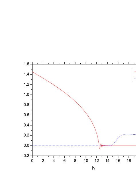
Figure 1: The evolution of the fields $\sigma$ and $\bar{\phi}$ for the case with $r=0.0301$ versus the number $N$ of e-foldings after the horizon exit of the pivot scale $k_{*}$, where we take $\sigma=1.45$, $\bar{\phi}=10^{-3}$, $\phi=10^{-8}$, $h=10^{-4}$, $\bar{h}=1.01\times 10^{-4}$, and $d\sigma/dt=-1.1074\times 10^{-6}$.

If we allow for a stronger running of the scalar spectral index, we may obtain larger values of $r$. For example, taking $\sigma_{*}=1.35$, $\kappa=1.75$, and $\beta=0.037$, we find $M=3.891\times 10^{-3}$, $C(\sigma_{*})=2.3479$, $\epsilon=0.00314$, $\eta=-0.00844$, $n_{\rm s}=0.9643$, $\alpha_{\rm s}=-0.03007$, and $r=0.0502$. In addition, we choose $m=3.891\times 10^{-5}$, $\lambda=0.1$, and $\gamma=10^{-6}$. With these choices, the pivot scale suffers about $10$ e-foldings during the first stage of inflation and, consequently, approximately another $41-42$ e-foldings must be provided by the second stage. This implies that $|\bar{\phi}_{\rm in}|$ lies in the range $0.38-0.40$. We verified numerically that the fulfillment of this requirement is indeed feasible. In Fig. 2, we depict the evolution of the fields $\sigma$ and $\bar{\phi}$ as functions of the number of e-foldings $N$ again starting from the point where the pivot scale $k_{*}$ exits the horizon for a particular choice of initial conditions at this point.

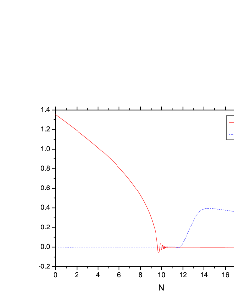
Figure 2: The evolution of the fields $\sigma$ and $\bar{\phi}$ for the case with $r=0.0502$ versus the number $N$ of e-foldings after the horizon exit of the pivot scale $k_{*}$, where we take $\sigma=1.35$, $\bar{\phi}=10^{-3}$, $\phi=10^{-8}$, $h=9\times 10^{-4}$, $\bar{h}=9.01\times 10^{-4}$, and $d\sigma/dt=-1.8523\times 10^{-6}$.

Needless to say that, changing the values of the input parameters of the model, we can easily achieve successful solutions with smaller values of the tensor-to-scalar ratio and that there is no particular fine-tuning of the parameters required in our model.

III.3 The formation of monopoles and cosmic strings

After the termination of the first stage of inflation, the system moves towards the semi-shifted path and the group $SU(2)_{\rm R}$ breaks spontaneously to a $U(1)$ subgroup by the nonzero value which the field $\Phi$ develops. This leads to the formation of superheavy magnetic monopoles. We can obtain a rough order of magnitude estimate of the mean distance between the monopoles and the antimonopoles, which is though adequate for our purposes here. We assume that, at production, this distance is $p\,(2\kappa M)^{-1}$ as determined by the relevant Higgs boson mass with $p\sim 1$ being a geometric factor. In the matter dominated period between the two inflationary stages, this distance increases by a factor $\sim(\kappa^{2}M^{4}/m^{2}M^{2})^{1/3}$, where $\kappa^{2}M^{4}$ and $m^{2}M^{2}$ are the classical potential energy densities on the trivial and the semi-shifted paths, respectively. The subsequent second inflationary stage stretches this distance by a factor $\exp{N_{2}}$, where $N_{2}$ is the number of e-foldings during this stage which is large but not huge – cf. Ref. intermediate . In the period of damped oscillations of the inflaton field, the monopole-antimonopole distance increases by another factor $\sim(m^{2}M^{2}/c(T_{\rm r})T_{\rm r}^{4})^{1/3}$, where $T_{\rm r}$ is the reheat temperature, which we take to be $10^{9}~{}{\rm GeV}$, and $c(T)=\pi^{2}g(T)/30$ with $g(T)$ being the effective number of massless degrees of freedom at cosmic temperature $T$. In the radiation dominated period which follows reheating, the monopole-antimonopole distance is multiplied by another factor $\sim T_{\rm r}/T\sim(4c(T)/3)^{1/4}T_{\rm r}\sqrt{t}$, where $t$ is the cosmic time. So this distance, in the radiation dominated period, becomes

$$\sim\left(\frac{4}{3}\right)^{\frac{1}{4}}c(T_{\rm r})^{-\frac{1}{3}}c(T)^{\frac{1}{4}}p\,(2\kappa M)^{-1}e^{N_{2}}\left(\frac{\kappa^{2}M^{4}}{T_{\rm r}^{4}}\right)^{\frac{1}{3}}T_{\rm r}t^{\frac{1}{2}}.$$ (54)

Equating this distance with the post-inflationary particle horizon $\sim 2t$, we find the time $t_{\rm H}$ (in $t_{\rm P}\equiv m_{\rm P}^{-1}\simeq 2.7027\times 10^{-43}~{}{\rm sec}$ units) at which the monopoles enter this horizon:

$$t_{\rm H}\sim\frac{p^{2}}{8\sqrt{3}}\,c(T_{\rm r})^{-\frac{2}{3}}c(T_{\rm H})^{\frac{1}{2}}e^{2N_{2}}\left(\frac{M}{\kappa\,T_{\rm r}}\right)^{\frac{2}{3}},$$ (55)

where $T_{\rm H}$ is the cosmic temperature at cosmic time $t_{\rm H}$.

The formation of monopoles is not the whole story though since our scenario leads to the generation of cosmic strings too. Indeed, after the end of the second inflationary stage, the system settles in one of the two distinct continua of SUSY vacua in Eqs. (3) and (4) with $\Phi_{\pm}\simeq\pm M$ in our case and a linear combination of the $U(1)_{B-L}$ gauge symmetry and the unbroken $U(1)$ subgroup of $SU(2)_{\rm R}$ breaks spontaneously leading to the production of local cosmic strings. These strings, if they survived after recombination, could have a small contribution to the CMBR power spectrum parametrized bevis by the dimensionless string tension $G\mu_{\rm s}$, where $G$ is Newton’s gravitational constant and $\mu_{\rm s}$ is the string tension, i.e. the energy per unit length of the string. Applying to our case the results of Ref. bevis , which considered local strings within the Abelian Higgs model in the Bogomol’nyi limit, we write, for the string tension,

$$\mu_{\rm s}=4\pi|\left<H\right>|^{2},$$ (56)

where $\left<H\right>$ is the VEV of $H$. Although the strings in our model are more complicated than in the Bogomol’nyi limit of the Abelian Higgs model, we think that the above estimate for the string tension is good enough for our purposes here.

In our case, the strings decay well before recombination and, thus, do not affect the CMBR. The reason is that they are mostly open strings connecting monopoles to antimonopoles. This is easily understood if we realize that the breaking of $SU(2)_{\rm R}\times U(1)_{B-L}$ to $U(1)_{Y}$ by $\left<H\right>$ and $\left<\bar{H}\right>$ is similar to the breaking of the electroweak gauge group and, thus, cannot lead to any topologically stable monopoles or strings – see Ref. trotta for a more detailed argument. It can only lead to the existence of topologically unstable dumbbell configurations dumbbell consisting of an open string with a monopole and an antimonopole at its two ends.

The strings, at any given time after their formation, can be thought of as random walks with a step of the order of the particle horizon walsh – to describe the evolution of this string network, we will follow closely this reference. They typically connect monopoles to antimonopoles, but unstable closed strings of limited size may also exist. As shown in Ref. walsh , at all times before the entrance of the monopoles into the horizon, there is of the order of one string segment per horizon and, thus, the ratio of the energy density $\rho_{\rm s}(t)$ of the string network to the total energy density $\rho_{\rm tot}(t)$ of the universe remains practically constant. At cosmic time $t_{\rm H}$, we have approximately one monopole-antimonopole pair per horizon volume $\sim(4\pi/3)(2t_{\rm H})^{3}$ connected by an almost straight string segment of the size of the horizon and energy $\sim\mu_{\rm s}2t_{\rm H}$. The energy density $\rho_{\rm s}(t_{\rm H})$ of the strings at cosmic time $t_{\rm H}$ is then $\sim 3G\mu_{\rm s}/2t_{\rm H}^{2}$. After this time, more and more string segments enter the horizon, but the length of each segment remains constant. Consequently, the system of string segments behaves like pressureless matter and, thus, $\rho_{\rm s}(t)\sim 3G\mu_{\rm s}/2(t_{\rm H}t^{3})^{1/2}$, which implies that the ‘relative string energy density’

$$\frac{\rho_{\rm s}(t)}{\rho_{\gamma}(t)}\sim 2G\mu_{\rm s}\left(\frac{t}{t_{\rm H}}\right)^{\frac{1}{2}}$$ (57)

($\rho_{\gamma}(t)$ is the photon energy density) increases with time – remember that we are in the radiation dominated era of the universe and, thus, $\rho_{\rm tot}(t)=\rho_{\gamma}(t)=c(T)\,T^{4}=3/4t^{2}$. The strings, finally, decay at cosmic time vilenkin

$$t_{\rm d}\sim(\Gamma G\mu_{\rm s})^{-1}2t_{\rm H},$$ (58)

where $\Gamma\sim 50$, by emitting gravitational waves with energy density $\rho_{\rm gw}(t_{\rm d})$ at production given by

$$\frac{\rho_{\rm gw}(t_{\rm d})}{\rho_{\gamma}(t_{\rm d})}\sim 2\left(\frac{2}{\Gamma}\right)^{\frac{1}{2}}(G\mu_{\rm s})^{\frac{1}{2}}$$ (59)

as one can infer from Eq. (57). Note that this formula also gives the maximal relative string energy density.

From Eq. (55) where we substitute the lowest value of the number of e-foldings $N_{2}$ and take $p=2$, we find that, for the two numerical examples presented, $t_{\rm H}\sim 4.76\times 10^{-7}~{}{\rm sec}$ and $1.04\times 10^{-4}~{}{\rm sec}$, respectively. In deriving these values, we take $g(T_{\rm r})=228.75$, which corresponds to the spectrum of the minimal SUSY SM, and $g(T_{\rm H})=40.75$ and $10.75$ in our two numerical examples, respectively. The above values of $g(T_{\rm H})$ are consistent with the effective number of massless degrees of freedom at the cosmic temperatures $T_{\rm H}$ corresponding to the values of the cosmic time $t_{\rm H}$ obtained. We see that the strings enter the horizon well before the time of big bang nucleosynthesis. Their decay time is $t_{\rm d}\sim 5.97\times 10^{-2}~{}{\rm sec}$ and $5.49~{}{\rm sec}$, in the two cases, as one can find from the corresponding dimensionless string tensions

$$G\mu_{\rm s}=\frac{|\left<H\right>|^{2}}{2}\simeq\frac{mM}{2\lambda}\simeq 3.19\times 10^{-7}\quad{\rm and}\quad 7.57\times 10^{-7}.$$ (60)

This means that the cosmic strings decay around the time of nucleosynthesis and, thus, well before recombination which takes place at a cosmic time $\sim 10^{13}~{}{\rm sec}$. As a consequence, they do not affect the CMBR. Their maximal relative energy density in the universe is $\sim 2.26\times 10^{-4}$ and $3.48\times 10^{-4}$ for our two numerical examples. So the cosmic strings remain always subdominant. In particular, they do not disturb nucleosynthesis at all.

Had the strings been around until the present time, an upper bound would have to be imposed on the dimensionless string tension in order to keep their contribution to the CMBR power spectrum at an acceptable level. For the Abelian-Higgs field theory model, this bound is found to be strings

$$G\mu_{\rm s}\lesssim 3.2\times 10^{-7}.$$ (61)

In our first numerical example, the dimensionless string tension $G\mu_{\rm s}$ given in Eq. (60) almost saturates the upper bound in Eq. (61), but violates the recent more stringent upper bound nano

$$G\mu_{\rm s}\lesssim 3.3\times 10^{-8}$$ (62)

from pulsar timing arrays, which also holds for strings surviving until the present time. Our second numerical example violates both the bounds in Eqs. (61) and (62). Thus, both our examples are only possible because the strings decay sufficiently early.

The value of the ratio of the energy density of the gravitational waves produced by the strings to that of the photons at the present cosmic time $t_{0}$ is found from Eq. (59) to be – cf. Ref. maggiore –

$$\frac{\rho_{\rm gw}(t_{0})}{\rho_{\gamma}(t_{0})}\sim 2\left(\frac{2}{\Gamma}\right)^{\frac{1}{2}}(G\mu_{\rm s})^{\frac{1}{2}}\left(\frac{3.9}{10.75}\right)^{\frac{4}{3}}.$$ (63)

The present abundance of these gravitational waves is then given by

$$\Omega_{\rm gw}h^{2}(t_{0})\sim\left(\frac{\rho_{\rm gw}(t_{0})}{\rho_{\gamma}(t_{0})}\right)\left(\frac{\rho_{\gamma}(t_{0})}{\rho_{\rm c}(t_{0})}\right)h_{0}^{2}\,,$$ (64)

where $\rho_{\rm c}(t_{0})$ is the present critical energy density of the universe and $h_{0}\simeq 0.7$ the present value of the Hubble parameter in units of ${\rm km~{}sec^{-1}~{}Mpc^{-1}}$. We find that, for our two numerical examples, $\Omega_{\rm gw}h^{2}(t_{0})\sim 2.18\times 10^{-9}$ and $3.35\times 10^{-9}$, respectively. The frequency $f(t_{\rm d})$ of these gravitational waves at production must be $\sim t_{\rm H}^{-1}$ since the length of the decaying strings is $\sim 2t_{\rm H}$ – see Ref. vilenkin . The present value of this frequency is then

$$f(t_{0})\sim t_{\rm H}^{-1}\left(\frac{t_{d}}{t_{\rm eq}}\right)^{\frac{1}{2}}\left(\frac{t_{\rm eq}}{t_{0}}\right)^{\frac{2}{3}},$$ (65)

where $t_{\rm eq}$ is the equidensity time at which matter starts dominating the universe. For the two numerical examples, this frequency turns out to be $\sim 1.06\times 10^{-4}~{}{\rm Hz}$ and $4.68\times 10^{-6}~{}{\rm Hz}$, respectively. Note that the estimate of the frequencies and abundances of the gravity waves presented here cannot be made much more accurate, but it can certainly be considered good enough for our purposes.

We see that the predicted frequencies of the gravitational waves are too high to yield any restrictions from CMBR considerations maggiore . They are also well above the range of frequencies probed by the pulsar timing array observations liu . So, the most recent stringent bound nano from these observations does not apply to our case. However, the frequency of the gravitational waves in our first numerical example lies marginally within the range to be probed by the future space-based laser interferometer gravitational-wave observatories such as the evolved laser interferometer space antenna/new gravitational-wave observatory (eLISA/NGO) lisa , which is expected to be able to detect values of $\Omega_{\rm gw}h^{2}(t_{0})$ as low as $4\times 10^{-10}$. Our overall conclusion is that the monopole-string system disappears without causing any trouble, but the gravitational waves that it generates may be probed by future space-based laser interferometer observations.

IV Conclusions

In view of the recent results joint1 ; joint2 indicating that appreciable values of the tensor-to-scalar ratio in the CMBR cannot be excluded, we addressed the question whether such values can be obtained in SUSY hybrid inflation models resulting from particle physics. To this end, we have considered a reduced version of the extended SUSY PS model of Ref. quasi , which was initially constructed for solving the $b$-quark mass problem of the simplest SUSY PS model with universal boundary conditions. The reason for focusing on this model is that it is known to support successful versions of hybrid inflation like the standard-smooth one stsmhi . This scenario is compatible with all the recent data even with a minimal Kähler potential, but predicts negligible values of the tensor-to-scalar ratio.

In the context of this particular particle physics model, we demonstrated that a two stage hybrid inflationary scenario which can predict values of the tensor-to-scalar ratio of the order of ${\rm few}\times 10^{-2}$ can be constructed. For the values of the parameters considered in this paper, the model in the global SUSY limit possesses practically two classically flat directions, the trivial and the semi-shifted semi one. The SUGRA corrections to the potential stabilize the trivial flat direction so that it becomes able to support a first stage of inflation. All the cosmological scales exit the horizon during this inflationary stage and our present horizon undergoes a limited number of e-foldings. The tensor-to-scalar ratio can acquire appreciable values as a result of sufficiently mild (i.e. non-catastrophic), but still appreciable SUGRA corrections combined with strong radiative corrections to the inflationary potential, while the value of the scalar spectral index remains acceptable. We can obtain values of the tensor-to-scalar ratio up to about $0.05$. Larger values would require unacceptably large running of the scalar spectral index.

The additional number of e-foldings required for solving the standard problems of hot big bang cosmology are generated by a second inflationary stage taking place along the semi-shifted path, where $U(1)_{B-L}$ is unbroken. This is possible since the semi-shifted direction, being almost orthogonal to the trivial path, is not affected by the strong radiative corrections on the trivial path and also because the SUGRA corrections on the semi-shifted path remain mild.

At the end of the first inflationary stage, the group $SU(2)_{\rm R}$ breaks spontaneously to a $U(1)$ subgroup and, thus, magnetic monopoles are formed. The subsequent spontaneous breaking of a linear combination of this $U(1)$ and $U(1)_{B-L}$ at the end of the second inflationary stage leads to the production of cosmic strings connecting these monopoles to antimonopoles. At later times, the monopoles enter the horizon and the string-monopole system decays into gravity waves well before recombination without leaving any trace in the CMBR. The resulting gravity waves, however, may be measurable in the future.

References

- (1) G. Lazarides, Lect. Notes Phys. 592, 351 (2002), hep-ph/0111328; J. Phys. Conf. Ser. 53, 528 (2006), hep-ph/0607032.
- (2) A.D. Linde, Phys. Rev. D 49, 748 (1994).
- (3) E.J. Copeland, A.R. Liddle, D.H. Lyth, E.D. Stewart, and D. Wands, Phys. Rev. D 49, 6410 (1994).
- (4) G.R. Dvali, Q. Shafi, and R.K. Schaefer, Phys. Rev. Lett. 73, 1886 (1994); G. Lazarides, R.K. Schaefer, and Q. Shafi, Phys. Rev. D 56, 1324 (1997).
- (5) G. Lazarides and C. Panagiotakopoulos, Phys. Rev. D 52, R559 (1995).
- (6) R. Jeannerot, S. Khalil, G. Lazarides, and Q. Shafi, J. High Energy Phys. 10, 012 (2000).
- (7) G. Lazarides and A. Vamvasakis, Phys. Rev. D 76, 083507 (2007).
- (8) R. Jeannerot, S. Khalil, and G. Lazarides, J. High Energy Phys. 07, 069 (2002).
- (9) M.E. Gomez, G. Lazarides, and C. Pallis, Nucl. Phys. B 638, 165 (2002).
- (10) G. Lazarides and C. Panagiotakopoulos, Phys. Lett. B 337, 90 (1994); S. Khalil, G. Lazarides, and C. Pallis, ibid. 508, 327 (2001).
- (11) B. Ananthanarayan, G. Lazarides, and Q. Shafi, Phys. Rev. D 44, 1613 (1991); Phys. Lett. B 300, 245 (1993).
- (12) D.N. Spergel et al., Astrophys. J. Suppl. 170, 377 (2007).
- (13) P.A.R. Ade et al. [Planck Collaboration], arXiv:1502. 01589.
- (14) C. Panagiotakopoulos, Phys. Rev. D 55, R7335 (1997); A.D. Linde and A. Riotto, ibid. 56, R1841 (1997); V.N. Şenoğuz and Q. Shafi, Phys. Lett. B 567, 79 (2003); ibid. 582, 6 (2004).
- (15) G. Lazarides and C. Pallis, Phys. Lett. B 651, 216 (2007); G. Lazarides, arXiv:0706.1436.
- (16) G. Lazarides and A. Vamvasakis, Phys. Rev. D 76, 123514 (2007).
- (17) P.A.R. Ade et al. [BICEP2 Collaboration], Phys. Rev. Lett. 112, 241101 (2014).
- (18) R. Flauger, J.C. Hill, and D.N. Spergel, J. Cosmol. Astropart. Phys. 08, 039 (2014); M. Cortês, A.R. Liddle, and D. Parkinson, arXiv:1409.6530.
- (19) R. Adam et al. [Planck Collaboration], arXiv:1409.5738.
- (20) M.J. Mortonson and U. Seljak, J. Cosmol. Astropart. Phys. 10, 035 (2014); C. Cheng, Q.G. Huang, and S. Wang, J. Cosmol. Astropart. Phys. 12, 044 (2014); L. Xu, arXiv:1409.7870.
- (21) P.A.R. Ade et al. [BICEP2/Keck and Planck Collaborations], Phys. Rev. Lett. 114, 101301 (2015).
- (22) T. Kobayashi and O. Seto, Mod. Phys. Lett. A 30, 1550106 (2015).
- (23) K.-Y. Choi and B. Kyae, Phys. Lett. B 735, 391 (2014).
- (24) M. Ur Rehman, Q. Shafi, and J. R. Wickman, Phys. Rev. D 83, 067304 (2011).
- (25) G. Lazarides, I.N.R. Peddie, and A. Vamvasakis, Phys. Rev. D 78, 043518 (2008).
- (26) C. Panagiotakopoulos, Phys. Lett. B 459, 473 (1999); Phys. Rev. D 71, 063516 (2005).
- (27) G. Lazarides and N.D. Vlachos, Phys. Rev. D 56, 4562 (1997).
- (28) G. Lazarides and Q. Shafi, Phys. Lett. B 148, 35 (1984).
- (29) N. Bevis, M. Hindmarsh, M. Kunz, and J. Urrestilla, Phys. Rev. D 75, 065015 (2007); ibid. 76, 043005 (2007); Phys. Rev. Lett. 100, 021301 (2008).
- (30) G. Lazarides, R. Ruiz de Austri, and R. Trotta, Phys. Rev. D 70, 123527 (2004).
- (31) Y. Nambu, Phys. Rev. D 10, 4262 (1974); Nucl. Phys. B 130, 505 (1977).
- (32) G. Lazarides, Q. Shafi, and T. Walsh, Nucl. Phys. B 195, 157 (1982).
- (33) A.Vilenkin and E.P.S. Shellard, Cosmic strings and other topological defects, Cambridge University Press, Cambridge, 2000.
- (34) P.A.R. Ade et al. [Planck Collaboration], Astron. Astrophys. 571, A25 (2014).
- (35) Zaven Arzoumanian et al. [NANOGrav Collaboration], arXiv:1508.03024.
- (36) M. Maggiore, Phys. Rep. 331, 283 (2000).
- (37) X.-J. Liu, W. Zhao, Y. Zhang, Z.-H. Zhu, arXiv:1509.03 524.
- (38) P. Amaro-Seoane et al., GW Notes 6, 4 (2013) [arXiv: 1201.3621].