Quantum gates by periodic driving

Abstract

Topological quantum computation has been extensively studied due to its robustness against decoherence. A conventional way to realize it is by adiabatic operations—it requires relatively long time to accomplish so that the speed of quantum computation slows down. In this work, we present a method to realize topological quantum computation by periodic driving. Compared to the adiabatic evolution, the total operation time can be regulated arbitrarily by the amplitude and frequency of the periodic driving. For the sinusoidal driving, we give an expression for the total operation time in the high-frequency limit. For the square wave driving, we derive an exact analytical expression for the evolution operator without any approximations, and show that the amplitude and frequency of driving field depend on its period and total operation time. This could provide a new direction in regulations of the operation time in topological quantum computation.

I introduction

Decoherence is an enemy of quantum computation, which is the loss of coherence due to the presence of environments. As a promising avenue to deal with the decoherence, topological quantum computations kitaev03 ; bonderson08 ; nayak08 ; miyake10 ; akhmerov10 ; xue14a ; MONG14 ; wootton14 employ two-dimensional quasiparticles called anyons, whose world lines cross over one another to form braids in a three-dimensional spacetime. Information encoded in the anyons is robust against local perturbations and quantum operations can be performed by braiding the non-Abelian anyons kitaev03 ; kitaev06 . The simplest example of the non-Abelian anyons is the Majorana fermions which are predicted to exist in fractional quantum Hall systems read00 , topological insulators hasan10 ; qi11 , solid state systems alicea12 , and semiconductor-superconductor hybrid systems sau2010 ; oreg10 ; lutchyn10 . The signatures of Majorana fermions have also been observed in experiments more recently das2012 ; mourik12 ; rokhinoson12 ; perge14 ; lee14 , which gives rise to an opportunity to encode a qubit by Majorana fermions in these materials.

A quantum task is often accomplished by a sequence of quantum operations rather than single quantum operation sau11 ; heck12 ; kraus13 ; laflamme14 ; ckarje11 ; chiu12 ; alicea11 . The total operation time increases linearly with the increasing of the number of operations. Considering the limit of the coherence time of quantum systems, long operation time is not favorable, even if the quantum topological computation is robust against perturbations. On the other hand, the time-periodic driving systems have been extensively studied in the past few years. Especially, several work oka09 ; kitagawa10 ; linder11 ; gu11 ; jiang11 ; liu13 ; katan13 ; rudner13 ; torres14 ; benito14 ; zhou14 ; piskunow14 ; usaj14 have shown that the topological properties can be changed in topologically trivial system by time-periodic driving (e.g., the existence of Floquet topological insulators or Floquet Majorana fermions). Recently, the Floquet Majorana fermions is realized by periodic driving fields in the system of coupled quantum dots proximity to a $s$-wave superconductor li2014 . More recently, it has been proposed to achieve the direct coupling between the topological and conventional qubits by periodic driving fields xue14b . In this paper we explore the possibility to regulate the total operation time by periodic driving For concreteness, the physical model of interest is the quantum dots coupled to the Majorana modes in a topological superconductor. Of course, this method can also be extended to the other quantum systems.

The paper is organized as follow. In Sect. II, we briefly introduce the topological quantum computation by adiabatic evolution. In Sect. III, we first recall the Floquet theory, then the periodic driving fields in the form of sinusoidal, square wave, and $\delta$-function kick are applied separately to modulate the total operation time for realizing the quantum operations. Finally we extend this method to other hybrid quantum systems in Sect. IV. The discussion and conclusion are given in Sect. V.

II quantum computation by adiabatical evolution

Recently, the adiabatic evolution has widely applied to the preparation and manipulation of Majorana fermions ckarje11 ; chiu12 ; kraus12 . In particular, it has been shown that topological quantum information processing becomes possible in the one-dimensional network alicea11 by adiabatically controlling the locally tunable gates which affect the chemical potential over a finite length of the wire. In following we describe the main idea of adiabatic evolution. That is, design a Hamiltonian $H_{1}$ whose ground state is the target state $|\Psi_{T}\rangle$ while the ground state $|\Psi_{0}\rangle$ of Hamiltonian $H_{0}$ is easily to prepared. Assume that there exists a quantum system satisfying the following Hamiltonian

$$H=[1-f(\frac{t}{T})]H_{0}+f(\frac{t}{T})H_{1},$$ (1)

where $f(t)$ is a slowly varying function of evolution time $t$ with $f(0)=0$ and $f(1)=1$. According to the adiabatic theorem, the quantum system evolves adiabatically from the initial (ground) state $|\Psi_{0}\rangle$ to the target (ground) state $|\Psi_{T}\rangle$ at time $t=T$.

In the present work, the physical model of interest consists of a quantum dot coupled to a semiconducting nanowire, as shown in Fig. 1(a). In a magnetic field, by proper spin orbit interaction and proximity coupling to a superconductor, the nanowire can exist the Majorana bound states in the topological phase lutchyn10 ; oreg10 ; alicea10 ; stoudenmire11 . Then the effective Hamiltonian (in the low-energy limit) for the quantum dot coupling to the Majorana mode reads flensberg11

$$H=\varepsilon(t)\hat{a}^{{\dagger}}\hat{a}+(v^{\ast}\hat{a}^{{\dagger}}-v\hat{a})\hat{\gamma}_{1},$$ (2)

where $a$ ($a^{{\dagger}}$) is the annihilation (creation) operator for the electron in quantum dot and the on-site energy $\varepsilon(t)$ for the quantum dot can be controlled by the gate voltage $V_{g}$. $v$ denotes the tunnel coupling between the quantum dot and the Majorana mode $\hat{\gamma}_{1}$. Without loss of generality we assume $v$ is an real number and take all physical parameters in units of $v$. Since the Majorana mode $\hat{\gamma}_{i}$ is Hermitian ($\hat{\gamma}^{{\dagger}}_{i}=\hat{\gamma}_{i}$ and $\hat{\gamma}^{2}_{i}=1$), we cannot use the number operator $\hat{\gamma}^{{\dagger}}_{1}\hat{\gamma}_{1}$ to count the occupation of the Majorana mode. Whereas, two Majorana modes can be combined to generate one ordinary fermion, e.g., $\hat{\gamma}_{1}=\hat{b}+\hat{b}^{{\dagger}}$ and $\hat{\gamma}_{2}=i(\hat{b}^{{\dagger}}-\hat{b})$. One can adopt the number operator $b^{{\dagger}}b$ of the ordinary fermion to count the Majorana modes.

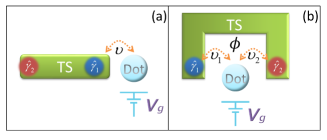
Figure 1: The setup for realizing the operation $P_{1}$.

Since the total parity of the electron in quantum dot and the ordinary fermion formed by Majorana modes is conserved, the Hamiltonian is block diagonal in the basis spanned by $\{|0\rangle_{F}|0\rangle_{D},|1\rangle_{F}|1\rangle_{D},|1\rangle_{F}|0\rangle_{D},|0\rangle_{F}|1\rangle_{D}\}$,

$$H=\left(\begin{array}[]{cccc}0&v&0&0\\ v&\varepsilon(t)&0&0\\ 0&0&0&v\\ 0&0&v&\varepsilon(t)\\ \end{array}\right),$$ (7)

where the state $|m\rangle_{F}|n\rangle_{D}$ ($m,n=0,1$) represents $m$ ordinary fermion formed by Majorana mode and $n$ electron in the quantum dot. In Ref. flensberg11 , it suggests that by adiabatically changing the values of $\frac{\varepsilon}{v}$ from $-\infty$ to $+\infty$, it can realize the operation $P_{1}$ which denotes the inversion of the occupation in ordinary fermion combined by the Majorana mode (i.e., $P_{1}=\hat{\gamma}_{1}$),

$$P_{1}(\sin\theta|0\rangle_{F}+\cos\theta|1\rangle_{F})=\sin\theta|1\rangle_{F}+\cos\theta|0\rangle_{F}.$$ (8)

Fig. 2 shows the different dynamics behaviors for distinct changing rate $\frac{\varepsilon}{v}$. It can be observed in Fig. 2(a) that the operation $P_{1}$ cannot be achieved perfectly since the changing of $\frac{\varepsilon}{v}$ does not satisfy the adiabatic condition very well (It cannot satisfy $V(t)\ll 1$ all the time). Thus the changing rate $\frac{\varepsilon}{v}$ should be small in order to meet the adiabatic condition, along with the increasing of operation time (cf. Fig. 2(c)-(d)). To implement the single qubit rotation or non-Abelian operation, one shall successively execute the operation $P_{1}$. Therefore the total operation time increases with the increasing of the number of operation $P_{1}$. In addition, it needs to point out that this Majorana based qubits may be susceptible to decoherence due to the electron tunnel coupling process budich12 ; goldstein11 ; rainis12 ; mazza13 . As a consequence, the adiabatic evolution is at a disadvantage in minimizing the influence of decoherence as far as possible. Recently, it is overcome by shortcuts to adiabaticity for the non-Abelian braiding with Y-junction structure karzig15 . In following it demonstrates that the situation can be changed by periodic driving.

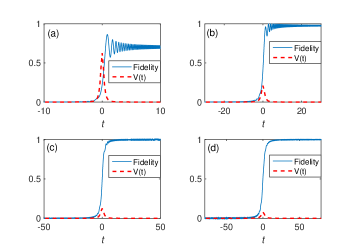
Figure 2: The time evolution of the system to obtain the operation $P_{1}$, where the fidelity is defined as $|\langle\psi(t)|\psi(T)\rangle|^{2}$. The expression of $V(t)$ is defined as, $V(t)=|\frac{\langle E_{1}(t)|\dot{E}_{2}(t)\rangle}{E_{1}(t)-E_{2}(t)}|$ where $|E_{i}(t)\rangle(i=1,2)$ is the instantaneous eigenstate with corresponding eigenvalue $E_{i}(t)$ in the even (or odd) subspace (The adiabatic condition can be written as $V(t)\ll 1$). The initial state is $|\psi(0)\rangle=\sin\theta|0\rangle_{F}+\cos\theta|1\rangle_{F}$ and the target state is $|\psi(T)\rangle=\sin\theta|1\rangle_{F}+\cos\theta|0\rangle_{F}$, $\theta=\frac{\pi}{6}$. We have set the on-site energy of the quantum dot increases with time linearly, e.g., $\varepsilon(t)=\frac{50}{T}t$. The operation time is $2T$ and the final value of $\varepsilon(t)$ is 50 during the time evolution. All parameters are in units of the tunnel coupling $v$. (a) $T=10$. (b) $T=30$. (c) $T=50$. (d) $T=80$. The larger $T$ means the smaller of the changing rate $\frac{\varepsilon}{v}$. One can find that the operation time for perfectly achieving the operation $P_{1}$ is about $2T=100$.

III quantum gates with periodic driving

III.1 Floquet theory

Let us first recall the Floquet theory briefly shirley65 . Provided that the system Hamiltonian has a time-periodic driving field, $H(t)=H(T+t)$, where $T$ is the period and the driving frequency reads $\omega=\frac{2\pi}{T}$. The Floquet theory asserts that the solutions of Schrödinger equation have the form $|\Phi_{n}(t)\rangle=e^{i\epsilon_{n}t}|\phi_{n}(t)\rangle$. $\epsilon_{n}$ is quasi-energy and the Floquet state $|\phi_{n}(t)\rangle$ has the property $|\phi_{n}(t)\rangle=|\phi_{n}(T+t)\rangle$. They are satisfied the following eigenvalue equation ($\hbar=1$)

$$[H(t)-i\frac{\partial}{\partial t}]|\phi_{n}(t)\rangle=\epsilon_{n}|\phi_{n}(t)\rangle,$$ (9)

where $H_{eff}=H(t)-i\frac{\partial}{\partial t}$ is defined as the Floquet Hamiltonian. To solve this equation it is very instructive to introduce an extend Hilbert space sambe73 of time-periodic functions with the inner product $\langle\langle\cdot|\cdot\rangle\rangle=\frac{1}{T}\int_{0}^{T}dt\langle\cdot|\cdot\rangle$.

With regard to the periodic driving system, it is necessary to make definite on the time-scales during the evolution. For the case of Floquet state $|\phi_{n}(t)\rangle$, since it has the same period with the driving field, it affects the system dynamics on short time-scale (in the high-frequency limit). What really affects the long time-scale of the system dynamics is the gap of the quasi-energies. Therefore, it is crucial to determine the evolution time through modulating the structure of quasi-energies in the periodic driving system.

III.2 Sinusoidal driving

We first consider the periodic modulation of the on-site energy for quantum dot with the sinusoidal form $\varepsilon(t)=\varepsilon_{0}\cos(\omega t)$, which can be created by a waveform generator. In order to obtain an approximate expression for the quasi-energy, we solve the time-dependent Schrödinger equation by standard perturbation theory holthaus92 ; creffield021 , where the tunneling Hamiltonian is regarded as the perturbation. Due to the total parity conservation it is convenient to study in the even parity (or odd parity) subspace. Then the Hamiltonian reduces $2\times 2$ matrix. Since $H_{\varepsilon}(t)=\varepsilon(t)a^{{\dagger}}a$ is diagonal, when substituting into Eq.(9), the eigenstates of $[H_{\varepsilon}(t)-i\frac{\partial}{\partial t}]$ can be readily given by

$$|\lambda_{1}(t)\rangle = (e^{i\lambda_{1}t},0)^{T},$$

$$|\lambda_{2}(t)\rangle = (0,e^{i\lambda_{2}t-i\frac{\varepsilon_{0}}{\omega}\sin\omega t})^{T},$$ (10)

where $\lambda_{i}$ ($i=1,2$) is the corresponding eigenvalue (i.e., quasi-energy). On the other hand, due to the period of Floquet states, one then can find that the zeroth order approximation of both quasi-energies are zero (modulo $\omega$). Thus the time-dependent eigenstates can be approximately viewed as time-independent eigenstates $|\lambda_{1}(t)\rangle=(1,0)^{T}$ and $|\lambda_{2}(t)\rangle\simeq(0,1)^{T}$ in the high-frequency limit ($\omega\gg 1$). The first order approximation of quasi-energies can be obtained via diagonalizing the perturbing matrix creffield021

$$\tilde{H}_{t}=\left(\begin{array}[]{cc}0&Q\\ Q^{\ast}&0\\ \end{array}\right),$$ (13)

where the matrix element $Q=\frac{v}{T}\int_{0}^{T}dte^{-i\frac{\varepsilon_{0}}{\omega}\sin\omega t}$ after some straightforward calculations. Consequently, the quasi-energies are calculated as $\epsilon_{1,2}=\pm|Q|$ (in the “first Brillouin zone”) and the corresponding eigenstates become $|\epsilon_{1,2}\rangle=\frac{1}{\sqrt{2}}(|\lambda_{1}(t)\rangle\pm|\lambda_{2}(t)\rangle)$. The gap of quasi-energies are then given by $\Delta=2|Q|$. In the light of the identity

$$e^{i\frac{\varepsilon_{0}}{\omega}\sin\omega t}=\sum_{n=-\infty}^{\infty}\mathcal{J}_{n}(\frac{\varepsilon_{0}}{\omega})e^{in\omega t},$$ (14)

where $\mathcal{J}_{n}$ is the $n$-order Bessel function, we can finally obtain the analytical expression for the quasi-energies gap $\Delta=2|v\mathcal{J}_{0}(\frac{\varepsilon_{0}}{\omega})|$.

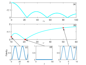
Figure 3: The gap of quasi-energies versus (a) the amplitude $\varepsilon_{0}$ when $\omega=10$, (b) the frequency $\omega$ when $\varepsilon_{0}=50$. The gap of quasi-energies approaches 2 when the driving frequency tends to 60 in panel (b). After that the gap increases slowly with the increasing of driving frequency. The dynamics evolution of periodic driving system with (c) $\omega=10$, (d) $\omega=20.8$, (e) $\omega=50$. All parameters are in units of the tunnel coupling $v$.

Fig. 3(a)-(b) demonstrate the relation between the driving field and the quasi-energies gap, while Fig. 3(c)-(e) show that the evolution time reduces with the increasing of the quasi-energies gap. Therefore, we can choose special evolution time for the periodic driving system by appropriately selecting the frequency and amplitude of driving field. An inspection of Fig. 3(a) also shows that the operation time varies with the decreasing of the amplitude of driving field when we fix a high frequency. Interestingly, there exists a special case that the quasi-energies of periodic driving system vanishes (namely the two quasi-energies approach degeneracy) by choosing the amplitude $\varepsilon_{0}$ and the driving frequency $\omega$ properly, which is known as coherent destruction of tunneling creffield02 ; creffield03 . As a consequence the state is localization so that it is invalid to achieve the operation $P_{1}$, as shown in Fig. 3(d).

Since the initial state can be approximately given by $|\psi(0)\rangle\simeq\frac{1}{\sqrt{2}}(|\epsilon_{1}\rangle-|\epsilon_{2}\rangle)$, the time evolution of periodic driving system approximately reads

$$|\psi(t)\rangle \simeq \frac{1}{\sqrt{2}}(e^{-i\epsilon_{1}t}|\epsilon_{1}\rangle-e^{-i\epsilon_{2}t}|\epsilon_{2}\rangle)$$ (15)

$$\simeq \cos{[\mathcal{J}_{0}(\frac{\varepsilon_{0}}{\omega})vt]}|\lambda_{2}\rangle-i\sin{[\mathcal{J}_{0}(\frac{\varepsilon_{0}}{\omega})vt]}|\lambda_{1}\rangle.$$

Hence the total operation time for realizing the operation $P_{1}$ approximately equals

$$\mathcal{T}\simeq\frac{\pi}{2v|\mathcal{J}_{0}(\frac{\varepsilon_{0}}{\omega})|}.$$ (16)

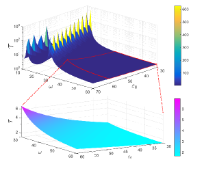
Figure 4: The total operation time $\mathcal{T}$ versus the amplitude $\varepsilon_{0}$ and the frequency $\omega$ of the driving field.

Fig. 4 depicts the relation between the total operation time and the amplitude as well as the frequency of the driving field. It suggests that one shall avoid the parameter regions with the coherent destruction of tunneling, since it takes long operation time to realize the operation $P_{1}$. Apart from this regions, the total operation time can be regulated within proper range. In addition, from the Eq. (15), one can find readily that the expression of fidelity is

$$F=\sin^{2}{[\mathcal{J}_{0}(\frac{\varepsilon_{0}}{\omega})vt]}=\frac{1}{2}(1-\cos{[2{\mathcal{J}_{0}(\frac{\varepsilon_{0}}{\omega})}vt]}).$$ (17)

Fig. 5 plots the relation between the gap of quasi-energies and the coefficients of fidelity in the exact and perturbation regime, respectively. It demonstrates that the perturbation results work extremely well in the high-frequency limit.

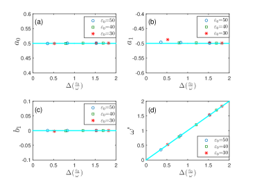
Figure 5: The coefficients (a) $a_{0}$, (b) $a_{1}$, (c) $b_{1}$, (d) $\omega^{\prime}$ of fidelity versus the gap of quasi-energies, where the expression of fidelity for curve-fitting is $F^{\prime}=a_{0}+a_{1}\cos{\omega^{\prime}t}+b_{1}\sin{\omega^{\prime}t}$. The lines represent the analytical solutions given by Eq. (17) with perturbation theory while the circles, squares, and stars represent exact results obtained by curve-fitting. Note that the curve-fitting has high degree of precision for the exact results since the values of R-square and Adjusted R-square approach unit ($\geq 99.37\%$) in MATLAB.

In order to check the validity of the perturbation theory, we plot the dynamics of the system with different driving frequencies. The results are given in Fig. 6. We observe that the dynamics is well in agreement with the results by perturbation theory when $\omega>10$ (in units of $v$), while it deviates seriously from the perturbation results when $\omega<10$ (in units of $v,$ see the pink dot-dash line in Fig. 6). As a result, one can employ the perturbation theory safely when the frequency of the driving field is at least an order of magnitude larger than the tunnel coupling.

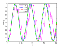
Figure 6: The evolution of the fidelity with different frequencies of driving field. We have set the quasi-energies gap $\Delta=2|v\mathcal{J}_{0}(\frac{\varepsilon_{0}}{\omega})|=1.0236$, thus the period of system dynamics is approximated to $T\simeq\frac{2\pi}{\Delta}=6.1383$ in the high-frequency limit, which is confirmed by the green solid line and red dash line.

As mentioned, the perturbation theory is not valid in the low-frequency limit, this gives rise to a question how the system behaviors in this limit. Now we go to explore this issue. When the driving frequency is small such that the adiabatic condition approximately holds (since the on-site energy changes slowly), we expected that the system dynamics, e.g., the fidelity, at the long time-scale would be periodic with period $T=\frac{2\pi}{\omega}$. As expectation, we find from the dash line in Fig. 7(a)-(c) that this is exact the case. Besides, one can observe that the high fidelity lasts a long time within a period when the driving frequency is small, see Fig. 7(a)-(d). The fidelity changes fast when the frequency of driving field is large (see Fig. 7(a), where the yellow lines and blue lines alter frequently). It also affects the dynamics when the amplitude of driving field is large, which is shown in Fig. 7(b). Fig. 7(c) illustrates how the offset energy affects the fidelity. Interestingly, the high fidelity lasts longer time (see the yellow region) when the offset on-site energy is larger.

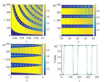
Figure 7: The fidelity as a function of the evolution time and the distinct parameters of driving field. The expression of driving field is $\varepsilon(t)=\varepsilon_{0}\cos\omega t-\xi$, where $\xi$ is the offset energy of driving field. (a) $\varepsilon_{0}=40,\xi=20$. (b) $\omega=0.05,\xi=0.5\varepsilon_{0}$. (c) $\varepsilon_{0}=40,\omega=0.05,\xi=\delta\varepsilon_{0}$. (d) $\varepsilon_{0}=40,\omega=0.04,\xi=20$. The dash lines are ploted by the function $t=\frac{2\pi}{\omega}n$, where $n$ is integer.

III.3 Square wave driving

It is believed that the periodic square wave driving fields are easily achieved in practice. In fact these driving fields have been studied extensively in time-periodic driving system. In particular, it has been shown in experiment silveri15 that the Stückelberg interference in a superconducting qubit is driven by the square wave form which we use in following. We first give the exact analytical expressions for system evolution operator without any approximations. The square wave driving for the on-site energy is expressed as

$$\varepsilon(t)=\left\{\begin{array}[]{rl}\varepsilon_{1},~{}~{}~{}~{}~{}~{}~{}~{}nT\leq t<t_{1}+nT,\\ \varepsilon_{2},~{}t_{1}+nT\leq t<(n+1)T,\\ \end{array}\right.$$ (20)

where $n=1,...,N$ and $t_{1}\in[0,T]$. Thus the system evolution operator $U$ of one period can be written as $U(T,0)=e^{-iH_{2}t_{2}}e^{-iH_{1}t_{1}}$ with $t_{2}=T-t_{1}$. After some lengthy algebra, one can obtain the expression of the evolution operator

$$U(T,0)=\frac{1}{x_{1}x_{2}}e^{-\frac{i}{2}D}\left(\begin{array}[]{cc}A&B+C\\ B-C&A\\ \end{array}\right),$$ (23)

where

$$A = -4v^{2}\sin\frac{x_{1}t_{1}}{2}\sin\frac{x_{2}t_{2}}{2}+(x_{1}\cos\frac{x_{1}t_{1}}{2}+i\varepsilon_{1}\sin\frac{x_{1}t_{1}}{2})$$

$$\cdot(x_{2}\cos\frac{x_{2}t_{2}}{2}+i\varepsilon_{2}\sin\frac{x_{2}t_{2}}{2}),$$

$$B = -2iv(x_{2}\cos\frac{x_{2}t_{2}}{2}\sin\frac{x_{1}t_{1}}{2}+x_{1}\cos\frac{x_{1}t_{1}}{2}\sin\frac{x_{2}t_{2}}{2}),$$

$$C = 2v(\varepsilon_{1}-\varepsilon_{2})\sin\frac{x_{1}t_{1}}{2}\sin\frac{x_{2}t_{2}}{2},$$

$$D = \varepsilon_{1}t_{1}+\varepsilon_{2}t_{2},~{}x_{1}=\sqrt{\varepsilon_{1}^{2}+4v^{2}},~{}x_{2}=\sqrt{\varepsilon_{2}^{2}+4v^{2}}.$$ (24)

At first we design the driving time $t_{1}$ ($t_{2}$) of the on-site energy $\varepsilon_{1}$ ($\varepsilon_{2}$) to satisfy $x_{1}t_{1}=\pi$ ($x_{2}t_{2}=\pi$), that is,

$$t_{1}=\frac{\pi}{\sqrt{4v^{2}+\varepsilon_{1}^{2}}},~{}~{}t_{2}=\frac{\pi}{\sqrt{4v^{2}+\varepsilon_{2}^{2}}},~{}~{}t_{1}+t_{2}=T.$$ (25)

Consequently, the period of the square wave driving is confirmed. According to Eq. (25), the evolution operator can be further simplified,

$$U(T,0)=\frac{-1}{x_{1}x_{2}}e^{-\frac{i}{2}D}\left(\begin{array}[]{cc}x_{3}&-x_{4}\\ x_{4}&x_{3}\\ \end{array}\right),$$ (28)

where $x_{3}=4v^{2}+\varepsilon_{1}\varepsilon_{2}$ and $x_{4}=2v(\varepsilon_{1}-\varepsilon_{2})$. After $N$ evolution periods, the final evolution operation becomes

$$U(\mathcal{T},0) = U^{N}(T,0)=\frac{1}{2}(\frac{-1}{x_{1}x_{2}})^{N}e^{-\frac{iND}{2}}$$ (31)

$$\cdot\left(\begin{array}[]{cc}r_{1}^{N}+r_{2}^{N}&-i(r_{1}^{N}-r_{2}^{N})\\ i(r_{1}^{N}-r_{2}^{N})&r_{1}^{N}+r_{2}^{N}\\ \end{array}\right),$$

where $r_{1}=x_{3}-ix_{4}=|r|e^{-i\theta},r_{2}=x_{3}+ix_{4}=|r|e^{i\theta},|r|=\sqrt{x_{3}^{2}+x_{4}^{2}},$ and $\tan\theta=\frac{x_{4}}{x_{3}}$. From the expression in Eq. (31), it clearly requires $r_{1}^{N}+r_{2}^{N}=0$ in order to realize the operation $P_{1}$ perfectly (up to a global phase factor). By making the vectors $r_{1}^{N}$ and $r_{2}^{N}$ produce a $\pi$-phase difference, that is, $N\theta-(-N\theta)=\pi$, one can readily obtain the number of evolution periods

$$N=\frac{\pi}{2\arctan\frac{2v(\varepsilon_{2}-\varepsilon_{1})}{4v^{2}+\varepsilon_{1}\varepsilon_{2}}}.$$ (32)

Note that according to Eq. (32) the number of evolution periods $N$ is not integer generally. Nevertheless it does not affect the main results because we can just take an integer nearest to $N$, as the fidelity increases slowly when it approaches 1. In turn, if one designates the period $T$ and the number of evolution periods $N$ in the periodic square wave driving system, the values of on-site energy $\varepsilon_{1}$ and $\varepsilon_{2}$ can be determined by Eq. (25) and Eq. (32) as well. It demonstrates the system evolution with distinct values of $\varepsilon_{1}$ and $\varepsilon_{2}$ in Fig. 8 (a)-(b), as well as the special period and the number of evolution periods in Fig. 8 (c)-(d). As expected, it can also realize the operation $P_{1}$ by square wave driving and we can modulate the period and the total operation time in this case.

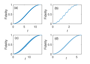
Figure 8: The system dynamics of distinct forms for square wave. (a) $\varepsilon_{1}=40$, $\varepsilon_{2}=60$. (b) $\varepsilon_{1}=10$, $\varepsilon_{2}=90$. (c) $T=0.3$, $N=60$. (d) $T=0.2$, $N=30$. The other two parameters are calculated by Eq.(25) and Eq.(32).

III.4 $\delta$-function kick

When $\varepsilon_{2}\rightarrow+\infty$, one can readily find in Eq.(25) that $t_{2}\rightarrow 0$. Then the square wave driving field reduces to periodic $\delta$-function kick, i.e.,

$$\varepsilon(t)=\varepsilon_{1}+\varepsilon_{2}\sum_{n=1}^{N}\delta(t-nT),$$ (33)

where $T$ is the driving period and can be calculated approximately as $T\simeq\frac{\pi}{\sqrt{4v^{2}+\varepsilon_{1}^{2}}}$. Therefore the total operation time for realizing the operation $P_{1}$ is approximatively

$$\mathcal{T} \simeq \frac{\pi^{2}}{2\sqrt{4v^{2}+\varepsilon_{1}^{2}}\arctan\frac{2v}{\varepsilon_{1}}}.$$ (34)

Note that the dynamics behavior is quite different from the absence of $\delta$-function kick, i.e., under a static driving field. In the static case, the evolution operator $U$ reads

$$U(t,0) = e^{-\frac{i\varepsilon_{1}t}{2}}\left(\begin{array}[]{cc}\cos\frac{xt}{2}+i\frac{\varepsilon_{1}}{x}\sin\frac{xt}{2}&-i\frac{2v}{x}\sin\frac{xt}{2}\\ -i\frac{2v}{x}\sin\frac{xt}{2}&\cos\frac{xt}{2}-i\frac{\varepsilon_{1}}{x}\sin\frac{xt}{2}\\ \end{array}\right),$$ (37)

$$x = \sqrt{\varepsilon_{1}^{2}+4v^{2}}.$$ (38)

In absence of $\delta$-function kick, the expression of fidelity for realizing the operation $P_{1}$ becomes $|\frac{2v}{x}\sin\frac{xt}{2}|^{2}$, where the maximum of fidelity is $|\frac{2v}{x}|^{2}$. One easily observes that it cannot obtain the operation $P_{1}$ when $\frac{2v}{x}\simeq 0$, i.e., the on-site energy $\varepsilon_{1}\gg 1$. However the situation changes in the presence of $\delta$-function kick and it can realize the operation $P_{1}$ regardless of the large value of on-site energy $\varepsilon_{1}$ (the value of $\varepsilon_{1}$ only determines the driving period). Especially, when we take away the $\delta$-function kick if the operation $P_{1}$ has been completed, the system is still stationary.

IV Application to other systems

The periodic driving method can be applied to the other structure of hybrid quantum dot-topological system. Here we apply it to a system described by the following Hamiltonian leijnse11 , as illustrated in Fig. 9,

$$H = \varepsilon(t)(\hat{a}_{\uparrow}^{{\dagger}}\hat{a}_{\uparrow}+\hat{a}_{\downarrow}^{{\dagger}}\hat{a}_{\downarrow})+V\hat{a}_{\uparrow}^{{\dagger}}\hat{a}_{\uparrow}\hat{a}_{\downarrow}^{{\dagger}}\hat{a}_{\downarrow}+(v_{1}^{\ast}\hat{a}_{\uparrow}^{{\dagger}}-v_{1}\hat{a}_{\uparrow})\hat{\gamma}_{1}$$ (39)

$$+(v_{2}^{\ast}\hat{a}_{\downarrow}^{{\dagger}}-v_{2}\hat{a}_{\downarrow})\hat{\gamma}_{2}.$$

$\varepsilon(t)$ is the on-site energy of the quantum dot. $v_{i}(i=1,2)$ denotes the tunnel coupling between the quantum dot and the Majorana mode $\hat{\gamma}_{i}$. In particular, the spin-up (labeled as $\uparrow$) and spin-down (labeled as $\downarrow$) electrons can only tunnel into the Majorana mode $\hat{\gamma}_{1}$ and $\hat{\gamma}_{2}$, respectively. $V$ represents the energy contributed by double occupation on the quantum dot. In the situation of large $V$, the quantum dot can only hold single electron.

Since the total parity (the electrons in quantum dot and the ordinary fermions formed by Majorana modes) of the hybrid system is conserved, we can restrict ourself in the even-parity subspace spanned by $\{|0\rangle_{F_{1}}|0\rangle_{F_{2}}|0\rangle_{D}$, $|1\rangle_{F_{1}}|1\rangle_{F_{2}}|0\rangle_{D}$, $|0\rangle_{F_{1}}|1\rangle_{F_{2}}|1_{\uparrow}\rangle_{D}$, $|0\rangle_{F_{1}}|1\rangle_{F_{2}}|1_{\downarrow}\rangle_{D}$, $|1\rangle_{F_{1}}|0\rangle_{F_{2}}|1_{\uparrow}\rangle_{D}$, $|1\rangle_{F_{1}}|0\rangle_{F_{2}}|1_{\downarrow}\rangle_{D},\}$, where the subscript $F_{i}(i=1,2)$ represents the ordinary fermions formed by Majorana modes. The matrix form of Hamiltonian then can be written as

$$H=\left(\begin{array}[]{cccccc}0&0&0&v_{2}&v_{1}&0\\ 0&0&v_{1}&0&0&v_{2}\\ 0&v^{\ast}_{1}&\varepsilon(t)&0&0&0\\ v^{\ast}_{2}&0&0&\varepsilon(t)&0&0\\ v^{\ast}_{1}&0&0&0&\varepsilon(t)&0\\ 0&v^{\ast}_{2}&0&0&0&\varepsilon(t)\\ \end{array}\right).$$ (46)

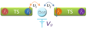
Figure 9: The setup for realizing entanglement between the convention qubit and topological qubit.

This quantum dot-Majorana system leijnse11 ; leijnse12 can be used to prepare entanglement between spin and topological qubits or quantum information transfer between spin and the topological qubits (even for the quantum logic gates) by the adiabatic evolution. We take the preparation of entanglement (denoting as the operation $P_{2}$) between the electron spin and Majorana modes as an example to exemplify how to manipulate the operation time by periodic square wave driving given in Eq. (20). The operation $P_{2}$ reads,

$$P_{2} (\sin\theta|0\rangle_{F_{1}}|0\rangle_{F_{2}}+\cos\theta|1\rangle_{F_{1}}|1\rangle_{F_{2}})|0\rangle_{D}$$ (47)

$$= \frac{v_{1}}{v}(\sin\theta|1\rangle_{F_{1}}|0\rangle_{F_{2}}+\cos\theta|0\rangle_{F_{1}}|1\rangle_{F_{2}})|1_{\uparrow}\rangle_{D}$$

$$+\frac{v_{2}}{v}(\sin\theta|0\rangle_{F_{1}}|1\rangle_{F_{2}}+\cos\theta|1\rangle_{F_{1}}|0\rangle_{F_{2}})|1_{\downarrow}\rangle_{D}.$$

where $v=\sqrt{v_{1}^{2}+v_{2}^{2}}$. As the Hamiltonian is a $6\times 6$ matrix, the analytical expression of the evolution operator $U(T,0)=e^{-iH_{2}t_{2}}e^{-iH_{1}t_{1}}$ is involved. Here we only give the equations that determine the period of the driving field and the total number of evolution periods, i.e.,

$$T = t_{1}+t_{2},$$

$$N = \frac{\pi}{2\arctan\frac{x^{\prime}_{4}}{x^{\prime}_{3}}},$$ (48)

where $t_{1}=\frac{\pi}{\sqrt{\varepsilon_{1}^{2}+4(v_{1}^{2}+v_{2}^{2})}}$, $t_{2}=\frac{\pi}{\sqrt{\varepsilon_{2}^{2}+4(v_{1}^{2}+v_{2}^{2})}}$, $x^{\prime}_{3}=\varepsilon_{1}\varepsilon_{2}+4v_{1}^{2}+4v_{2}^{2}$, and $x^{\prime}_{4}=2(\varepsilon_{2}-\varepsilon_{1})\sqrt{v_{1}^{2}+v_{2}^{2}}$. Fig. 10 plots the fidelity of realizing operation $P_{2}$ as a function of the evolution time by the adiabatic evolution and the periodic square wave driving, respectively. Again, we find that the operation time for adiabatic evolution requires relatively long time since it must satisfy the adiabatic condition while the operation time and the period of the square wave driving can be regulated.

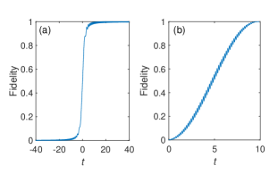
Figure 10: (a) Realizing the operation $P_{2}$ by the adiabatic evolution. The on-site energy of the quantum dot increases with time slowly, $\varepsilon(t)=1.25t$. (b) Realizing the operation $P_{2}$ by the periodic square-wave driving. $\varepsilon_{1}=30,\varepsilon_{2}=50.$ $\theta=\frac{\pi}{6}$, $v_{1}=v_{2}=\frac{1}{\sqrt{2}}$. All parameters are in units of $v$.

V discussion and conclusion

In the last section, we have studied how to implement the operation $P_{1}$ by periodically driving the on-site energy of the quantum dot. For a single operation $P_{1}$, it is far from sufficient to permit quantum computation. We next briefly discuss how to realize an arbitrary rotation for a qubit by successively executing the operation $P_{1}$ twice.

As shown in Fig. 1(b), the system Hamiltonian of interest reads

$$H = \varepsilon(t)\hat{a}^{{\dagger}}\hat{a}+(|v_{1}|e^{-i\theta_{1}}\hat{a}^{{\dagger}}-|v_{1}|e^{i\theta_{1}}\hat{a})\hat{\gamma}_{1}$$ (49)

$$+(|v_{2}|e^{-i\theta_{2}}\hat{a}^{{\dagger}}-|v_{2}|e^{i\theta_{2}}\hat{a})\hat{\gamma}_{2},$$

where we have introduced a phase $\theta_{1}$ ($\theta_{2}$) into the tunnel coupling $v_{1}$ ($v_{2}$) in the Hamiltonian. Defining the operator $\hat{c}=\hat{a}e^{i\theta_{1}}$, $z=\sqrt{|v_{1}|^{2}+|v_{2}|^{2}}$, $z_{1}=\frac{|v_{1}|}{z}$, and $z_{2}=\frac{|v_{2}|}{z}$, the Hamiltonian (49) becomes,

$$H=\varepsilon(t)\hat{c}^{{\dagger}}\hat{c}+z(\hat{c}^{{\dagger}}-\hat{c})(z_{1}\hat{\gamma}_{1}+z_{2}\hat{\gamma}_{2}),$$ (50)

where the phase difference $\theta_{1}-\theta_{2}$ equals $2n\pi$ ($n$ is integer and the phase can be modulated by the magnetic flux $\phi$). The form of Eq.(50) is the same as Eq.(2) if we redefine a new Majorana mode $\hat{\gamma}_{12}=z_{1}\hat{\gamma}_{1}+z_{2}\hat{\gamma}_{2}$, where the tunnel coupling is denoted by $z$. Clearly, the operation $P_{1}=\hat{\gamma}_{12}$ in this notation. Consider the two level system spanned by $\{|0\rangle_{F},|1\rangle_{F}\}$, then we can express the Majorana operators in terms of Pauli matrices $\{\sigma_{x},\sigma_{y},\sigma_{z}\}$, i.e., $\hat{\gamma}_{1}=\sigma_{x}$, $\hat{\gamma}_{2}=\sigma_{y}$, $\hat{\gamma}_{1}\hat{\gamma}_{2}=i\sigma_{z}$. By successively executing the operation $P_{1}$ twice with different relative tunnel coupling strengthes between modes $z_{1}$ and $z_{2}$, the total operation becomes $P=\hat{\gamma}_{12}\hat{\gamma}_{12}^{\prime}=(z_{1}\hat{\gamma}_{1}+z_{2}\hat{\gamma}_{2})(z_{1}^{\prime}\hat{\gamma}_{1}+z_{2}^{\prime}\hat{\gamma}_{2})=(z_{1}z_{1}^{\prime}+z_{2}z_{2}^{\prime})+i(z_{1}z_{2}^{\prime}-z_{1}^{\prime}z_{2})\sigma_{z}$, which is exactly an arbitrary rotation around the $z$-axis.

Due to the conservation of the total parity, a qubit shall be encoded by four Majorana modes bravyi06 . The Majorana-based qubit can be realized by the generalization model in Fig. 1(b), which describes a system consisting of three quantum dots coupling to four Majorana modes ($\hat{\gamma}_{1}$, $\hat{\gamma}_{2}$, $\hat{\gamma}_{3}$, $\hat{\gamma}_{4}$) in the topological superconductor with comb structure. In the even-parity subspace spanned by $\{|0\rangle_{F_{1}}|0\rangle_{F_{2}}$, $|1\rangle_{F_{1}}|1\rangle_{F_{2}}\}$, the operation $P=\hat{\gamma}_{12}\hat{\gamma}_{12}^{\prime}$ is in fact the rotation around the $z$-axis, and the operation $P=\hat{\gamma}_{23}\hat{\gamma}_{23}^{\prime}$ is the rotation around the $x$-axis ($\hat{\gamma}_{23}=z_{2}\hat{\gamma}_{2}+z_{3}\hat{\gamma}_{3}$), where the ordinary fermion $F_{1}$ ($F_{2}$) is formed by the Majorana modes $\hat{\gamma}_{1}$ and $\hat{\gamma}_{2}$ ($\hat{\gamma}_{3}$ and $\hat{\gamma}_{4}$).

Generally speaking, the tunnel coupling between the quantum dot and the Majorana mode depends on both the differences among the on-site energies and the tunnel barriers. By making use of the periodic driving on the on-site energy of the quantum dot, the tunnel coupling would change consequently. Reminding that we can employ additional electrostatic gates to manipulate the tunnel barriers, the tunnel coupling can keep a constant in practise, even the on-site energies change. Indeed, the possibility of controlling the tunnel coupling in semiconductor nanowire has been experimentally shown recently nadjperge10 . So, we believe that in the near future it is also possible to manipulate the gates such that the tunnelling rate remains unchanged in our case, especially with the periodic square pulses (since it has only two distinct values of on-site energy).

In conclusion, we have proposed a method to regulate the total operation time of quantum computation, which can be achieved by periodic driving. By solving the time-dependent Schrödinger equation with perturbation expansion, we have given an expression of the quasi-energies and elucidated the relationship between the total operation time and quasi-energies in the high-frequency limit. As a result, the operation time can be manipulated by designing the amplitude and frequency of the driving field. For the case of low-frequency limit, due to the invalidity of the perturbation theory, we study the dynamical behaviors by numerical simulations. We find the results approach those given by adiabatic evolution. Different from the adiabatic evolution, the system in the low-frequency limit manifests more intricate behaviors and the operation time can also be regulated by the driving field. In particular, the total time that the high fidelity lasts are closely related to the frequency and offset energy of driving field. For the case of periodic square wave driving, we have derived an analytical expression for the evolution operator without any approximations. By this expression, we can calculate the amplitude of square wave driving fields with fixed operation time and period of driving fields. We have also discussed the realization of quantum operations by the $\delta$-kick, which can be treated as a deformed square wave driving. The periodic driving can also be applied to the other quantum system—it opens up a new avenue in manipulations of operation time in topological quantum computations.

References

- (1) A. Y. Kitaev, Ann. Phys. 303, 2 (2003).
- (2) C. Nayak, S. H. Simon, A. Stern, M. Freedman, and S. Das Sarma, Rev. Mod. Phys. 80, 1083 (2008).
- (3) P. Bonderson, M. Freedman, and C. Nayak, Phys. Rev. Lett. 101, 010501 (2008).
- (4) A. Miyake, Phys. Rev. Lett. 105, 040501 (2010).
- (5) A. R. Akhmerov, Phys. Rev. B 82, 020509 (2010).
- (6) Z. Y. Xue, L. B. Shao, Y. Hu, S. L. Zhu, and Z. D. Wang, Phys. Rev. A 88, 024303 (2013).
- (7) R. S. K. Mong, D. J. Clarke, J. Alicea, N. H. Lindner, P. Fendley, C. Nayak, Y. Oreg, A. Stern, E. Berg, K. Shtengel, and M. P. A. Fisher, Phys. Rev. X 4, 011036 (2014).
- (8) J. R. Wootton, J. Burri, S. Iblisdir, and D. Loss, Phys. Rev. X 4, 011051 (2014).
- (9) A. Y. Kitaev, Ann. Phys. 321, 2 (2006).
- (10) N. Read and D. Green, Phys. Rev. B 61, 10267 (2000).
- (11) M. Z. Hasan and C. L. Kane, Rev. Mod. Phys. 82, 3045 (2010).
- (12) X. L. Qi and S. C. Zhang, Rev. Mod. Phys. 83, 1057 (2011).
- (13) J. Alicea, Rep. Prog. Phys, 75, 076501 (2012).
- (14) J. D. Sau, R. M. Lutchyn, S. Tewari, and S. Das Sarma, Phys. Rev. Lett. 104, 040502 (2010).
- (15) Y. Oreg, G. Refael, and F. von Oppen, Phys. Rev. Lett. 105, 177002 (2010).
- (16) R. M. Lutchyn, J. D. Sau, and S. Das Sarma, Phys. Rev. Lett. 105, 077001 (2010).
- (17) A. Das, Y. Ronen, Y. Most, Y. Oreg, M. Heiblum, and H. Shtrikman, Nat. Phys. 8, 887 (2012).
- (18) V. Mourik, K. Zuo, S. M. Frolov, S. R. Plissard, E. P. A. M. Bakkers, and L. P. Kouwenhoven, Science 336, 1003 (2012).
- (19) L. P. Rokhinson, X. Liu, and J. K. Furdyna, Nat. Phys. 8, 795 (2012).
- (20) S. N. Perge, I. K. Drozdov, J. Li, H. Chen, S. Jeon, J. Seo, A. H. MacDonald, B. A. Bernevig, and A. Yazdani, Science, 346, 602 (2014).
- (21) E. J. H. Lee, X. Jiang, M. Houzet, R. Aguado, C. M. Lieber, and S. De Franceschi, Nat. Nanotech. 9, 79 (2014).
- (22) J. D. Sau, D. J. Clarke, and S. Tewari, Phys. Rev. B 84, 094505 (2011).
- (23) B. van Heck, A. R. Akhmerov, F. Hassler, M. Burrello, and C. W. J. Beenakker, New J. Phys. 14, 035019 (2012).
- (24) C. V. Kraus, P. Zoller, and M. A. Baranov, Phys. Rev. Lett. 111, 203001 (2013).
- (25) C. Laflamme, M. A. Baranov, P. Zoller, and C. V. Kraus, Phys. Rev. A 89, 022319 (2014).
- (26) D. J. Clarke, J. D. Sau, and S. Tewari, Phys. Rev. B 84, 035120 (2011).
- (27) C. K. Chiu, M. M. Vazifeh, and M. Franz, arXiv:1403.0033 (2014).
- (28) J. Alicea, Y. Oreg, G. Refael, F. von Oppen, and M. P. A. Fisher, Nat. Phys. 7, 412 (2011).
- (29) T. Oka and H. Aoki, Phys. Rev. B 79, 081406 (2009).
- (30) T. Kitagawa, E. Berg, M. Rudner, and E. Demler, Phys. Rev. B 82, 235114 (2010).
- (31) N. H. Lindner, G. Refael, and V. Galitski, Nat. Phys. 7, 490 (2011).
- (32) Z. Gu, H. A. Fertig, D. P. Arovas, and A. Auerbach, Phys. Rev. Lett. 107, 216601 (2011).
- (33) L. Jiang, T. Kitagawa, J. Alicea, A. R. Akhmerov, D. Pekker, G. Refael, J. I. Cirac, E. Demler, M. D. Lukin, and P. Zoller, Phys. Rev. Lett. 106, 220402 (2011).
- (34) D. E. Liu, A. Levchenko, and H. U. Baranger, Phys. Rev. Lett. 111, 047002 (2013).
- (35) Y. T. Katan, D. Podolsky, Phys. Rev. Lett. 110, 016802 (2013).
- (36) M. S. Rudner, N. H. Lindner, E. Berg, and M. Levin, Phys. Rev. X 3, 031005 (2013).
- (37) L. E. F. Foa Torres, P. M. Perez-Piskunow, C. A. Balseiro, G. Usaj, Phys. Rev. Lett. 113, 266801 (2014).
- (38) M. Benito, A. Gomez-Leon, V. M. Bastidas, T. Brandes, and G. Platero, Phys. Rev. B 90, 205127 (2014).
- (39) M. Lababidi, I. I. Satija, and E. Zhao, Phys. Rev. Lett. 112, 026805 (2014).
- (40) P. M. Perez-Piskunow, G. Usaj, C. A. Balseiro, and L. E. F. Foa Torres, Phys. Rev. B 89, 121401 (2014).
- (41) G. Usaj, P. M. Perez-Piskunow, L. E. F. Foa Torres, and C. A. Balseiro, Phys. Rev. B 90, 115423 (2014).
- (42) Y. Li, A. Kundu, F. Zhong, and B. Seradjeh, Phys. Rev. B 90, 121401 (2014).
- (43) Z. Y. Xue, M. Gong, J. Liu, Y. Hu, S. L. Zhu, and Z. D. Wang, Sci. Rep. 5, 12233 (2015).
- (44) C. V. Kraus, S. Diehl, P. Zoller, and M. A. Baranov, New J. Phys. 14, 113036 (2012).
- (45) J. Alicea, Phys. Rev. B 81, 125318 (2010).
- (46) E. M. Stoudenmire, J. Alicea, O. A. Starykh, and M. P. A. Fisher, Phys. Rev. B 84, 014503 (2011).
- (47) K. Flensberg, Phys. Rev. Lett. 106, 090503 (2011).
- (48) J. C. Budich, S. Walter, and B. Trauzettel, Phys. Rev. B 85, 121405 (2012).
- (49) G. Goldstein and C. Chamon, Phys. Rev. B 84, 205109 (2011).
- (50) D. Rainis and D. Loss, Phys. Rev. B 85, 174533 (2012).
- (51) L. Mazza, M. Rizzi, M. D. Lukin, and J. I. Cirac, Phys. Rev. B 88, 205142 (2013).
- (52) T. Karzig, F. Pientka, G. Refael, and F. von Oppen, Phys. Rev. B 91, 201102 (2015).
- (53) J. H. Shirley, Phys. Rev. 138, B979 (1965).
- (54) H. Sambe, Phys. Rev. A 7, 2203 (1973).
- (55) M. Holthaus, Z. Phys. B: Condens. Matter 59, 251 (1992).
- (56) C. E. Creffield and G. Platero, Phys. Rev. B 65, 113304 (2002).
- (57) C. E. Creffield and G. Platero, Phys. Rev. B 66, 235303 (2002).
- (58) C. E. Creffield, Phys. Rev. B 67, 165301 (2003).
- (59) M. P. Silveri, K. S. Kumar, J. Tuorila, J. Li, A. Vepsäläinen, E. V. Thuneberg, and G. S. Paraoanu, New J. Phys. 17 043058 (2015).
- (60) M. Leijnse and K. Flensberg, Phys. Rev. B 86, 104511 (2012).
- (61) M. Leijnse and K. Flensberg, Phys. Rev. Lett. 107, 210502 (2011).
- (62) S. Bravyi,Phys. Rev. A 73, 042313 (2006).
- (63) S. Nadj-Perge, S. M. Frolov, E. P. A. M. Bakkers, and L. P. Kouwenhoven, Nature 468, 1084 (2010).