Robust state transfer with high fidelity in spin-1/2 chains by Lyapunov control

Abstract

Based on the Lyapunov control, we present a scheme to realize state transfer with high fidelity by only modulating the boundary spins in a quantum spin-1/2 chain. Recall that the conventional transmission protocols aim at non-stationary state (or information) transfer from the first spin to the end spin at a fixed time. The present scheme possesses the following advantages. First, the scheme does not require precise manipulations of the control time. Second, it is robust against uncertainties in the initial states and fluctuations in the control fields. Third, the controls are exerted only on the boundary sites of the chain. It works for variable spin-1/2 chains with different periodic structures and has well scalability. The feasibility to replace the control fields by square pules is explored, which simplifies the realization in experiments.

I introduction

Quantum information processing (QIP) has been extensively studied in the past decades. One of the main challenges in actual physical implementations of QIP is to transfer quantum information between different elements in quantum networks. In this respect, spin chain systems as quantum channelsbose07 ; kay10 ; apollaro13 to transfer information play an important role in QIP. It is believed that almost all spins would participate in the dynamics of an unmodulated spin chain bose03 due to spin-spin couplings, leading to dispersions of the chain that are harmful for quantum state transfer. Recently, several strategies have been proposed to avoid such dispersions (see, e.g., christandl04 ; fitzsimons06 ; venuti07 ; gualdi08 ; feldman09 ; banchi10 ; ping13 ; zwich13 ; banchi11 ). The first approach is mainly based on modulating coupling strengths between nearest neighbors to reduce the effect of dispersion wang11 ; bruderer12 ; vinet12 . The second depends on the weak interaction of boundary spins to the remainders (bulk spins), making the bulk spins almost un-excited during the time evolution. The dynamics in the second method can be viewed as an effective Rabi oscillation between the boundary spins bruderer12 ; paganelli06 ; wojcik07 ; venuti07pra . In the other sort of schemes, such as modulating the Larmor frequencies on sites feldman10 or adding external potentials giorgi13 to the spin chain, perfect state transfer can be obtained only for a fixed time. This means that a precise control on the evolution time is strictly required to obtain high fidelity state transfer. Once there exist errors in the coherent time evolution, the fidelity decreases sharply.

One important progress to take the disorders into account was made in Ref. yao11 , where an robust state transmission in random unpolarized spin chains was proposed. This proposal is immune to some significant types of disorders and does not need to manipulate individual spins. In contrast, by manipulating the individual spin-spin couplings, Zwick and co-workers zwick11 ; zwick12 investigated the performance for quantum state transfer and showed its robustness against static perturbations.

Lyapunov-based control technique has attracted many attentions due to its powerful applications in manipulating quantum states in quantum systems alessandro07 ; beauchard07 ; kuang08 ; coron09 ; wang09 ; wang10 ; hou12 ; yi09 . To apply the Lyapunov control, a function of the target state called Lyapunov function $V$ has to be specified, where the control field $f(t)$ is designed to guarantee the Lyapunov function decreasing monotonously, i.e., $\dot{V}\leq 0$. The merit of the Lyapunov control is that the target is asymptotically approached, which means the manipulation time is not important. In this paper, we apply the Lyapunov-based control technique to the quantum state transfer from one boundary spin to another. We show that by manipulating the interaction strengths between the boundary spins and the bulk spins in an one-dimensional spin-1/2 chain, the quantum state transfer can be realized. To show the robustness of this control, we numerically calculate the performance under the effect of external perturbations.

The paper is organized as follows. In section II, we present a general formalism for state transfer in a spin-1/2 chain by Lyapunov control. In section III, we select a specific eigenstate of the spin-1/2 chain for state transfer. The control fields are designed and the robustness against fluctuations is investigated in section IV. The scalability of the state transfer in such a spin-1/2 chain and the improvement on the control fields are briefly discussed in section V. Finally, we give a conclusion in section VI.

II general formalism for state transfer in spin-1/2 chain

We start by considering an one-dimensional spin-1/2 chain with modulated XY interactions between nearest neighbors. The free Hamiltonian can be written as,

$$H_{0}^{xy}=\frac{1}{2}\sum_{m=1}^{M-1}D_{m}(S_{m}^{x}S_{m+1}^{x}+S_{m}^{y}S_{m+1}^{y})-\frac{1}{2}\sum_{m=1}^{M}\Omega_{m}S_{m}^{z},$$ (1)

where $\Omega_{m}$ is the Larmor frequency and $D_{m}$ denotes the coupling strength between the $m$-th and $(m+1)$-th spins. $S_{m}^{i}(i=x,y,z)$ is the Pauli matrix and $M$ is the length of spin-1/2 chain. We label the first spin and the end spin by $1$ and $M$, respectively. Clearly, $[H_{0}^{xy},S^{z}]=0$ where $S^{z}=\sum_{m=1}^{M}S_{m}^{z}$, means that the total number of spin up (down) is conserved. When quantum information is encoded on the state of spin up and spin down in the spin-1/2 chain, the state transfer can be equivalent to information transfer from the first spin to the end spin.

By Jordan-Wigner transformation, the spin Hamiltonian $H_{0}^{xy}$ can be mapped into a spinless fermions Hamiltonian,

$$H_{0}=\sum_{m=1}^{M-1}D_{m}(c_{m}^{{\dagger}}c_{m+1}+c_{m+1}^{{\dagger}}c_{m})+\sum_{m=1}^{M}\Omega_{m}c_{m}^{{\dagger}}c_{m},$$ (2)

where $c_{m}$ ($c_{m}^{{\dagger}}$) represents the annihilation (creation) operator of spinless fermion at site $m$. Due to $[H_{0},\sum_{m=1}^{M}c_{m}^{{\dagger}}c_{m}]=0$, one can decompose the Hilbert space $\mathcal{H}$ into subspaces $\mathcal{H}=\sum_{j}\mathcal{H}_{j}$, each of them such as $\mathcal{H}_{j}$, possessing a fixed number of spinless fermions $j$. We then choose the subspace $\mathcal{H}_{0}$ and $\mathcal{H}_{1}$ for the state transfer, in which it has one excitation at most. Apparently, the dimension of subspace $\mathcal{H}_{1}$ is equal to the number of spins in the chain and we denote the state with a single excitation at site $m$ by $|\textbf{m}\rangle$. The Hamiltonian $H_{0}$ can then be written in a matrix form in the basis $\{|\textbf{m}\rangle\}$,

$${H_{0}}=\left(\begin{array}[]{ccccccc}\Omega_{1}&D_{1}&0&0&\cdots&0&0\\ D_{1}&\Omega_{2}&D_{2}&0&\cdots&0&0\\ 0&D_{2}&\Omega_{3}&D_{3}&\cdots&0&0\\ 0&0&D_{3}&\Omega_{4}&\cdots&0&0\\ \vdots&\vdots&\vdots&\vdots&\ddots&\vdots&\vdots\\ 0&0&0&0&\cdots&\Omega_{M-1}&D_{m-1}\\ 0&0&0&0&\cdots&D_{M-1}&\Omega_{M}\\ \end{array}\right),$$ (3)

where the vacuum state $|\textbf{0}\rangle=|00\cdots 0\rangle$, and $|\textbf{m}\rangle=c_{m}^{{\dagger}}|\textbf{0}\rangle=|0\cdots 01_{m}0\cdots 0\rangle$ note1 . In the following, we study the problem of state transfer by using this matrix form of system Hamiltonian.

To be specific, the state transfer can be obtained by free evolution of the Hamiltonian $H_{0}$ bose03 ; christandl04 ; bruderer12 ; feldman10 . It can be formulated as follows: The initial state of the first spin is $\alpha|0\rangle+\beta|1\rangle$, while the remaining spins are in spin down state,

$$|\psi(0)\rangle = \alpha|0_{1}0\cdot\cdot\cdot 00_{M}\rangle+\beta|1_{1}0\cdot\cdot\cdot 00_{M}\rangle$$ (4)

$$= \alpha|\textbf{0}\rangle+\beta|\textbf{1}\rangle,$$

where $|\alpha|^{2}+|\beta|^{2}=1$. After a fixed evolution time $t=T$, the system would evolve to,

$$|\psi(T)\rangle = \alpha|0_{1}0\cdot\cdot\cdot 00_{M}\rangle+\beta|0_{1}0\cdot\cdot\cdot 01_{M}\rangle$$ (5)

$$= \alpha|\textbf{0}\rangle+\beta|\textbf{M}\rangle.$$

Those proposals need to control the evolution time precisely to get perfect state transfer. Especially, the final state in those proposals is not a steady state. In the following, by Lyapunov control, we show that in the spin-1/2 chain one can realize steady state transfer with high fidelity. The control process can be illustrated as,

$$|\psi(0)\rangle=\alpha|\textbf{0}\rangle+\beta|\textbf{1}\rangle\xLongrightarrow[\texttt{control}]{\texttt{Lyapunov}}|\psi(T)\rangle=\alpha|\textbf{0}\rangle+\beta|\lambda_{f}\rangle,$$ (6)

where $|\lambda_{f}\rangle$ denotes the target state and one of eigenstates of Hamiltonian $H_{0}$ at the same time. Because $|\textbf{0}\rangle$ is the ground state of spin-1/2 chain, and we choose the control Hamiltonian such that the ground state remains unchange in the dynamics, the state transfer mainly focuses on steering the initial state $|\textbf{1}\rangle$ into the target state $|\lambda_{f}\rangle$.

We should point out that the quantum information encoded in the first spin is almost perfectly transferred to the end spin in our system, like the other protocols bose03 ; christandl04 ; fitzsimons06 ; venuti07 ; gualdi08 ; feldman09 ; banchi10 ; ping13 ; zwich13 ; banchi11 did for state transfer. The difference is that our resulting state is the eigenstate $|\lambda_{f}\rangle$ rather than the state $|\textbf{M}\rangle$ in equation (5). This change has many advantages as we mentioned in the abstract, the price we have to pay is the state (or information) is not localized well at the end spin, leading to imperfect state transfer. This can be improved by designing the Hamiltonain as we show below.

When adding control fields $f_{k}(t)$ with control Hamiltonians $H_{k}$ into the system, the time evolution of spin-1/2 chain satisfies the following Schrödinger equation ($\hbar=1$):

$$|\dot{\psi}\rangle=-i\Big{[}H_{0}+\sum_{k=1}^{K}f_{k}(t)H_{k}\Big{]}|\psi\rangle.$$ (7)

In Lyapunov control, the target state $|\psi_{T}\rangle$ is usually chosen as an eigenstate of the free Hamiltonian $H_{0}$, such that when completing the control, the target state should be a steady state,

$$H_{0}|\psi_{T}\rangle=\lambda_{f}|\psi_{T}\rangle,$$ (8)

where $\lambda_{f}$ is the eigenvalue corresponding to the eigenstate $|\psi_{T}\rangle$. To design the control fields, a Lyapunov function has to be chosen. By the merit of Lyapunov control, we choose the Lyapunov function as follows,

$$V=\langle\psi|P|\psi\rangle,$$ (9)

where the hermitian operator $P$ is time independent. Furthermore, $P$ should commute with the Hamiltonian $H_{0}$, i.e., $[H_{0},P]=0$. With this definition, the time derivative of $V$ is

$$\dot{V}=\sum_{k=1}^{K}f_{k}(t)\langle\psi|i[H_{k},P]|\psi\rangle.$$ (10)

The construction of the operator $P$ is flexible, such as

$$P=p_{f}|\lambda_{f}\rangle\langle\lambda_{f}|+\sum_{i\neq f}p_{i}|\lambda_{i}\rangle\langle\lambda_{i}|,$$ (11)

where $|\lambda_{i}\rangle$ ($i=1,...,N$) is the eigenstate of Hamiltonian $H_{0}$ with eigenvalue $\lambda_{i}$. To transfer a quantum state successfully, we should choose $p_{i}$ to meet the condition that $p_{f}<p_{i}$ yi09 . Obviously, when the system arrives at the target state, $V$ reaches its minimum. Simple algebra shows that the control fields $f_{k}(t)=-A_{k}\langle\psi|i[H_{k},P]|\psi\rangle$ with $A_{k}>0$ can assure $\dot{V}\leq 0$. As a consequence, those control fields would transfer the quantum state from the spin 1 to the spin $M$.

Strictly speaking, the proposal of state transfer should work for any state at spin 1, i.e., $\alpha$ and $\beta$ in equation (4) could take any value. A good measure to quantify the performance of the state transfer then should take an average over all $\alpha$ and $\beta$. With this consideration, we introduce the following averaged fidelity $F(t)$ to quantify the state transfer bose03 ,

$$F(t)=\frac{|f_{M,1}(t)|}{3}\cos\tau+\frac{|f_{M,1}(t)|^{2}}{6}+\frac{1}{2},$$ (12)

where $\tau=\arg|f_{M,1}(t)|$ and $f_{M,1}(t)=\langle\textbf{M}|e^{-iHt}|\textbf{1}\rangle$. We set $\cos\tau=1$ hereafter since $\tau$ is controllable.

III target state

Conventionally, the target state should be an eigenstate of the free Hamiltonian, such that when finishing the control, the target state is stationary. However, the perfect goal of this proposal is to transfer a state from one side $|\textbf{1}\rangle$ to another $|\textbf{M}\rangle$. To this extent, our proposal cannot be taken as a proposal for state transfer, nevertheless, when $|\lambda_{f}\rangle$ is almost the same as $|\textbf{M}\rangle$, our proposal works. So, the purpose of this section is to choose the parameters such that $|\langle\textbf{M}|\lambda_{f}\rangle|$ is as high as possible (i.e., making the occupation of spin $M$ approach 1 in the eigenstate $|\lambda_{f}\rangle$). In the following, we calculate the eigenstates of Hamiltonian $H_{0}$ in the spin-1/2 chain where the Larmor frequencies $\Omega_{m}$ and coupling strength $D_{m}$ in equation (3) are periodic function of sites with period $l$, i.e. $\Omega_{m}=\Omega_{m+l}$ and $D_{m}=D_{m+l}$. To be specific, we set the period $l=3$. The solutions of eigenvalues and eigenstates of this general linear chain with open boundary have been given in appendix feldman06 . We select a specific eigenstate of the Hamiltonian $H_{0}$ so that the target state satisfies the condition $|\langle\textbf{M}|\lambda_{f}\rangle|\sim 1$. By the results given in the appendix, the components of this specific eigenstate $u$ can be expressed analytically as follow,

$$u_{3i-1} = \frac{D_{1}}{\lambda_{v}-\Omega_{2}}u_{3i-2},$$

$$u_{3i} = 0,$$

$$u_{3i+1} = -\frac{D_{1}D_{2}}{(\lambda_{v}-\Omega_{2})D_{3}}u_{3i-2},$$ (13)

where $i=1,...,n$ and the corresponding eigenvalue $\lambda_{v}=\frac{1}{2}[(\Omega_{1}+\Omega_{2})\pm\sqrt{(\Omega_{1}-\Omega_{2})^{2}+4D_{1}^{2}}]$. From the expression of eigenstate $u$, it is not hard to find that the occupations on each site (defined as $|u_{i}|^{2}$) are determined by the coupling strengths $D_{k}(k=1,2,3)$ and the Larmor frequencies $\Omega_{1}$ and $\Omega_{2}$. If the conditions $|\frac{D_{1}}{\lambda_{v}-\Omega_{2}}|<1$ and $|\frac{D_{1}D_{2}}{(\lambda_{v}-\Omega_{2})D_{3}}|<1$ are both satisfied simultaneously, the values of $|u_{3i-2}|^{2}$ and $|u_{3i-1}|^{2}$ decrease monotonously, respectively. In this case, the occupation on the spin $M$ is maximum or minimum, hence it is possible to let this eigenstate $u$ serve as the target state. In particular, $f(D_{1})=\frac{D_{1}}{\lambda_{v}-\Omega_{2}}$ is a monotonic increasing function with the argument $D_{1}$. Thus, the value of $D_{1}$ should be small in order to obtain high fidelity state transfer, i.e., the boundary spins should be weakly coupled to the bulk of spin-1/2 chain.

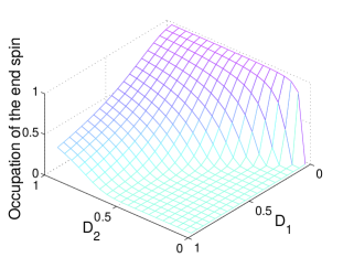
Figure 1: The occupation of the end spin as a function of interaction strength $D_{1}$ and $D_{2}$. We choose the total number of spins $M=29$. The other parameters are in units of the coupling strengths $D_{3}=1$, and $\Omega_{1}=1.5$, $\Omega_{2}=\Omega_{3}=0.75$.

Instead of the quadratic couplings investigated in Ref. bruderer12 , we here consider periodic couplings for the following reasons. Firstly, the system is robust against small perturbations due to the existence of gaps; Secondly, it can describe topological materials like topological insulators. In addition, systems with periodic couplings are not rare in practice. Figure 1 shows the occupation of end spin $M$ as a function of the coupling strengths $D_{1}$ and $D_{2}$. As expected, the occupation of end spin $M$ becomes large when $D_{1}$ is small. For simplicity, we choose $D_{1}=0.15$, $D_{2}=D_{3}=1$, $\Omega_{1}=1.5$, and $\Omega_{2}=\Omega_{3}=0.75$ in the following numerical calculation.

IV realization of state transfer by lyapunov control

IV.1 Lyapunov function

In this section, we first investigate the free evolution of the system starting with initial state $|\textbf{1}\rangle$ without any external controls, that is, $H_{k}=0$ in equation (7). The results are presented in figure 2. One can find that the state of system stays at $|\textbf{1}\rangle$ with a high fidelity. This is a merit of our spin-1/2 chain: not only the final state but the initial state are almost stationary when the system does not subject to any external controls. In other words, it can not realize state transfer without external controls in our system since the system is almost still at the initial state.

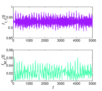
Figure 2: Free evolution, namely, the time evolution without any controls. (a) The fidelity $f_{1,1}(t)=\langle\textbf{1}|e^{-iH_{0}t}|\textbf{1}\rangle$ versus time $t$. (b) The fidelity $f_{M,1}(t)=\langle\textbf{M}|e^{-iH_{0}t}|\textbf{1}\rangle$ versus time $t$.

Next, we control the coupling strengths between the boundary spins and the bulk spins, i.e.,

$$H_{k}=c_{k}^{{\dagger}}c_{k+1}+c_{k+1}^{{\dagger}}c_{k},~{}~{}k=1,M-1.$$ (14)

The coefficients of the hermitian operator $P$ are chosen as $p_{i}=\lambda_{i}$ and $p_{f}=-3$. The dynamics behavior of fidelity $F$ is illustrated as a function of the control time $t$ in figure 3. It approaches a steady value about 96.84% when the control finishes, thus we can conclude that we have realized state transfer with high fidelity.

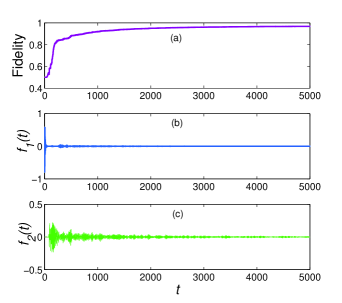
Figure 3: (a) Evolution of the fidelity $F$ versus control time $t$. We have set $A_{k}=1$ and $P_{f}=-3$ to guarantee the condition $P_{f}<P_{i}$ with $P_{i}=\lambda_{i}$. (b) The control field $f_{1}(t)$. (c) The control field $f_{2}(t)$.

IV.2 Robustness of state transfer

So far, we have demonstrated that high fidelity of state transfer can be obtained by Lyapunov control without any fluctuations in the control field and uncertainties in the free Hamiltonian $H_{0}$. In practice, however, the parameters in the free Hamiltonian $H_{0}$ are not easy to acquire precisely, and fluctuations of the control fields might occur in experimental manipulations, which would lead to errors in the state transmission. In this section, we focus on this issue. We begin with analyzing robustness against the uncertainty in the free Hamiltonian $H_{0}$, which can be represented by $\delta\cdot H_{0}$,

$$H_{0}\rightarrow H_{0}+\delta\cdot H_{0}.$$

Here $\delta$ is independent random quantities manifested in coupling strengths $\delta\cdot D_{k}$ or Larmor frequencies $\delta\cdot\Omega_{k}$ ($k=1,2,3$). Since the fidelity of this system will be impacted by the perturbations seriously when the control time takes too long, we truncate the control time $t=1000$ in the numerical calculations while the fidelity can approach 92%. As we only control the boundary coupling strengths to achieve state transfer, we emphasize on analyzing the influence of boundary parametric fluctuations on the fidelity at first.

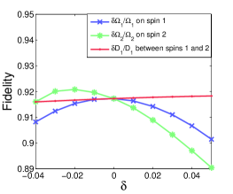
Figure 4: The behavior of fidelity versus disorder of parameters related to spin 1 and spin 2. We have fixed the control time $t=1000$.

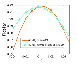
Figure 5: The behavior of fidelity versus disorder of the magnetic field $\Omega_{1}$ on spin 28 and the coupling strength between spins 28 and 29. We have fixed the control time $t=1000$.

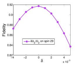
Figure 6: The behavior of fidelity versus disorder of the magnetic field $\Omega_{2}$ on spin 29. We have fixed the control time $t=1000$.

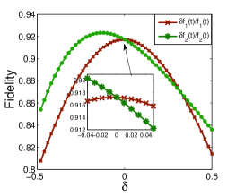
Figure 7: The behavior of fidelity versus disorder of the control fields. We have fixed the control time $t=1000$.

Figure 4 shows the fidelity of state transfer as a function of uncertainties in the first or second spins. Those perturbations have slight effects on the fidelity of state transfer since those parameters primarily affect the control field $f_{1}(t)$, and it only plays a significant role in the beginning while almost vanishes at later time, as seen in figure 3. Figure 5 and figure 6 show the relationship between the fidelity and the uncertainties related to the $28$th or $29$th spins. Those parameters have much impact on the fidelity due to the closely connection with the control field $f_{2}(t)$ and the occupation of end spin in target state. In addition, it can be found in those figures that the fidelity might be even higher when the uncertainties are very small. The reason can be understood as follows. In the ideal situation, the fidelity increases monotonously during the time evolution. Small uncertainties/fluctuations might not change the sign but change the amplitude of control fields, leading to a slight oscillation in the value of fidelity. As a consequence, the fidelity might increase due to these uncertainties.

This can also be used to explain why a higher fidelity can be reached when fluctuations exist in the control fields $f_{k}(t)$, since the fidelity sharply depends on the sign rather than the amplitude of control fields in figure 7. We find from the inset that the influence of the control field $f_{2}(t)$ is more sensitive than that of the control field $f_{1}(t)$ when fluctuations are small. It can be explained by an observation in figure 3 that there still exists small control field $f_{2}(t)$ when $t>1000$ while the amplitude of control field $f_{1}(t)$ almost vanishes at that time. For its insensitive in the fluctuations of control fields, making the interaction time long would be in favor of obtaining high fidelity of state transfer. On the other hand, when considering the disorder of other physical parameters such as coupling strengths $\delta\cdot D_{k}$ or Larmor frequency $\delta\cdot\Omega_{k}$, the distribution of eigenstates of the Hamiltonian $H_{0}$ might change. Hence the final state might not be a steady state and evolves even though the control fields disappear (or turn off). So the fidelity of state transfer might deteriorate with the increasing of interaction time. As a consequence, one should trade off the disorders of different parameters to truncate an appropriate control time in order to obtain a relatively high fidelity.

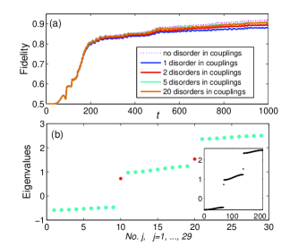
Figure 8: (Color online) (a)Fidelity as a function of time. The dot line denotes the fidelity in the case without disorders, while the solid lines show the fidelity with disorders. Each line is an average over 100 simulations, where each simulation is obtain by introducing no disorder, 1, 2, 5 and 20 disorders. (b)The eigenvalues of Hamiltonian when the total spins $M=29$. The inset shows the eigenvalues of total spins $M=209$.

Now, we turn to study the effect of disorder in (the whole spin chain) couplings on the performance of the state transfer. To this end, we adopt the same control fields and initial state as in the case without disorders, but change randomly the couplings from $D_{j}$ to $D_{j}^{r}=(1+\epsilon)D_{j}$, where $D_{j}$ is the original couplings in the above analysis and $j$ is spin site index. $\epsilon$ is a randomly chosen number in the interval [-0.05, 0.05]. In other words, we explore the effect of disorders by re-simulating the state transfer with $D_{j}^{r}$ instead of $D_{j}$, and $D_{j}^{r}$ changes randomly at each point of time for a randomly chosen spin site. We simulate $n$ disorders ($n=1,2,5,20$) existing simultaneously in the system and show the results in figure 8(a). One can discover that the scheme is robust against disorders in the couplings. The disorders in the on-site energy would have similar effects on the performance.

An interesting observations is that more disorders might benefit the performance of the state transfer. This might relate to the random number $\epsilon$ being created in [-0.05, 0.05], i.e., the average of $\epsilon$ is closely to zero. The physics behind the robustness of the scheme is that small random disorders in the couplings cannot close the gaps in the system since it has nontrivial topological property lang12 , as shown in figure 8(b). As a result, the boundary states appear in the system, making our control protocol robust, which is the essential reason why we choose the periodical system.

V scalability and discussion

Until now, we have just considered a chain with $M=29$ spins. A natural question arises that whether the interaction time increases with the increasing of the spin number. Since the interaction time is also closely related to the amplitude of control fields $f_{k}(t)$, we set $A_{k}=1$ in the expression of $f_{k}(t)$ and study this problem by numerical calculation. Figure 9 demonstrates the relation between the interaction time and different total number of spins while the fidelity of state transfer reaches 0.93. It is observed that the interaction time increases approximately linearly with the total number of spins.

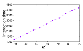
Figure 9: The interaction time $t$ versus different total number of spins $M$. The interaction time finishes when the fidelity of state transfer reaches 0.93. All the other parameters are the same with figure 3.

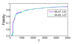
Figure 10: Evolution of the fidelity $F$ versus control time $t$. The parameters (the pink solid line) are $\Omega_{1}=\Omega_{5}=1.5$, $\Omega_{2}=\Omega_{3}=\Omega_{4}=0.75$, $D_{1}=0.15$, $D_{3}=0.5$, $D_{2}=D_{4}=D_{5}=1$. The parameters of the cyan dash line are the same to figure 3 except for the total number of spins $M=59$.

Although the general formulas of exact diagonalization of matrix with period ($l>3$) in Larmor frequencies and coupling strengths is given in Ref. feldman06 , the analytical expressions are complicated. For this reason, we will employ the numerical calculation to investigate whether the Lyapunov control is suited to the case for the period $l>3$. Numerical simulations show that, it is possible to obtain high fidelity state transfer in a spin-1/2 chain with 47 sites of period $l=5$, and the fidelity can approach 94.97% when completing the control, as shown in figure 10. The another feature in figure 10 is that the dynamics behaviors of the fidelity with $M=47$ and $l=5$ almost coincides with the case of $M=59$ and $l=3$, indicating that the interaction time does not linearly increase with the total number of spins in different periodic structure of spin-1/2 chains. As the Lyapunov function, i.e., $V=p_{f}|\langle\psi|\lambda_{f}\rangle|^{2}+\sum p_{i}|\langle\psi|\lambda_{i}\rangle|^{2}$, represents the weighted average between the state of system and distinct eigenstates of Hamiltonian $H_{0}$. The variation of Lyapunov function reflects that the control fields mainly modulate the state transition between the eigenstates of Hamiltonian $H_{0}$. Thus the interaction time is connected with the characteristic spectrum of Hamiltonian $H_{0}$ rather than the total number of spins. Once the free Hamiltonian $H_{0}$ of spin-1/2 chain contains an eigenstate whose occupation mainly locates at the end spin, there should exist a Lyapunov function for the control fields to control the state transition between eigenstates of Hamiltonian $H_{0}$. As a result, it can realize state transfer by the Lyapnouv control, of course, the fidelity of state transmission must be closely linked to the characteristic spectrum of Hamiltonian $H_{0}$.

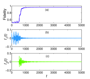
Figure 11: All parameters and the expression for control function are the same as in figure 3 except for the control Hamiltonian.

In a practical situation, the control Hamiltonians which exchange the interaction between the boundary spins and its neighbors in equation (14) might be difficult to obtain. An alternative way of realizing state transfer is to control the Larmor frequencies at the boundary spins, namely, the control Hamiltonians are chosen as $H_{1}=c^{{\dagger}}_{1}c_{1}$ and $H_{2}=c^{{\dagger}}_{M}c_{M}$. Figure 11 shows the performance of fidelity when controlling the Larmor frequencies at the boundary spins. Indeed, it also can realize state transfer. Furthermore, we can replace the fast time-varying control fields by square wave pulses, which reduces the difficulty in experiments. The square wave pulses are given by

$$f_{k}(t)=\left\{\begin{array}[]{rl}F^{\prime}_{k},~{}~{}~{}f_{k}(t)>0,\\ -F^{\prime}_{k},~{}~{}~{}f_{k}(t)<0.\\ \end{array}\right.$$ (17)

By these square wave pulses, in figure 12, we show that the target can be reached with high fidelity as well.

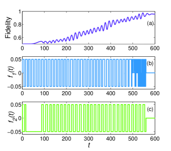
Figure 12: All physical parameters are the same as in figure 11 except for the control fields. We set $F^{\prime}_{k}=0.05$. The control is terminated when the fidelity arrived at 0.96.

VI conclusion

In conclusion, by Lyapunov control technique, we have proposed a scheme for state transfer in the spin-1/2 chain. The controls are exerted on the couplings between the boundary spins and its neighbors. It also works by manipulating the Larmor frequencies of the boundary spins. The difference between our proposal and the others is that the resulting state here is an eigenstate of the system Hamiltonian, hence it is stationary and it does not require to finish the transfer at a fixed time. In addition, the proposal is robust against many types of perturbations and disorders since those perturbations could not close the gaps of the system. This proposal can also be generalized to a structure with periodicity $l>3$, provided that the chain has an eigenstate localized at the boundary spin (the receiver). For chains which have no eigenstate perfectly localized at the boundary spin, a high fidelity state transfer can be obtained as well by elaborately designing the parameters of the spin-1/2 chain. Finally, we have shown that replacing the fast time-varying control fields with square wave pulses are possible, which simplifies the experimental realization.

APPENDIX

The diagonalization of a matrix representing the Hamiltonian of spin-1/2 chain with total spins $M$ ($M=nl+d$), Larmor frequencies $\Omega_{m}$, coupling strength $D_{m}$, periodicity $l$, $l>d\geq 0$ and $l>1$, has been given in Ref. feldman06 ; schultz69 ; feldman05 . When $l=3$ and $d=2$, the matrix reads,

$${H}=\left(\begin{array}[]{ccccccc}\Omega_{1}&D_{1}&0&0&\cdots&0&0\\ D_{1}&\Omega_{2}&D_{2}&0&\cdots&0&0\\ 0&D_{2}&\Omega_{3}&D_{3}&\cdots&0&0\\ 0&0&D_{3}&\Omega_{1}&\cdots&0&0\\ \vdots&\vdots&\vdots&\vdots&\ddots&\vdots&\vdots\\ 0&0&0&0&\cdots&\Omega_{1}&D_{1}\\ 0&0&0&0&\cdots&D_{1}&\Omega_{2}\\ \end{array}\right).$$ (18)

The $3n$-distinct eigenvalues $\lambda_{v}$ of this Hamiltonian can be obtained by solving following equation,

$$(\lambda_{v}-\Omega_{1})(\lambda_{v}-\Omega_{2})(\lambda_{v}-\Omega_{3})-(\lambda_{v}-\Omega_{2})D_{3}^{2}$$

$$-(\lambda_{v}-\Omega_{1})D_{2}^{2}-(\lambda_{v}-\Omega_{3})D_{1}^{2}=2D_{1}D_{2}D_{3}\cos(\frac{\pi k}{n+1}),$$ (19)

where $k=1,2,...,n.$ The corresponding eigenvectors $u_{j}=(u_{1,j},u_{2,j},u_{3,j},...,u_{3n+1,j},u_{3n+2,j})^{T}$ are

$$U_{1,j} = \frac{(\lambda_{v}-\Omega_{2})\mathscr{D}_{3}^{T}+D_{1}\mathscr{D}_{2}^{T}}{(\lambda_{v}-\Omega_{1})(\lambda_{v}-\Omega_{2})-D_{1}^{2}}\cdot U_{3,j},$$

$$U_{2,j} = \frac{(\lambda_{v}-\Omega_{1})\mathscr{D}_{2}^{T}+D_{1}\mathscr{D}_{3}^{T}}{(\lambda_{v}-\Omega_{1})(\lambda_{v}-\Omega_{2})-D_{1}^{2}}\cdot U_{3,j},$$

$$U_{3,j} = \Big{(}\sin(\frac{\pi[\frac{j+2}{3}]}{n+1}),\sin(\frac{2\pi[\frac{j+2}{3}]}{n+1}),...,\sin(\frac{n\pi[\frac{j+2}{3}]}{n+1})\Big{)}^{T}$$

with

$$U_{1,j} = (u_{1,j},u_{4,j},...,u_{3n-2,j},u_{3n+1,j})^{T},$$

$$U_{2,j} = (u_{2,j},u_{5,j},...,u_{3n-1,j},u_{3n+2,j})^{T},$$

$$U_{3,j} = (u_{3,j},u_{6,j},...,u_{3n,j})^{T},$$

$${\mathscr{D}_{2}}=\left(\begin{array}[]{ccccc}D_{2}&0&\cdots&0&0\\ 0&D_{2}&\cdots&0&0\\ \vdots&\vdots&\ddots&\vdots&\vdots\\ 0&0&\cdots&D_{2}&0\\ \end{array}\right),$$

$${\mathscr{D}_{3}}=\left(\begin{array}[]{ccccc}0&D_{3}&0&\cdots&0\\ 0&0&D_{3}&\cdots&0\\ \vdots&\vdots&\vdots&\ddots&\vdots\\ 0&0&0&\cdots&D_{3}\end{array}\right).$$

Here $[x]$ represents the largest integer less than or equal to $x$, the superscript “$T$” denotes transposition and $j=1,2,...,3n$. $\mathscr{D}_{2}$ and $\mathscr{D}_{3}$ are $n\times(n+1)$ matrices.

The other two eigenvalues $\lambda_{v}$ satisfy the following equation,

$$(\lambda_{v}-\Omega_{1})(\lambda_{v}-\Omega_{2})-D_{1}^{2}=0.$$ (20)

The corresponding eigenvector $u_{j}$ can be expressed

$$u_{3i-1,j} = \frac{D_{1}}{\lambda_{v}-\Omega_{2}}u_{3i-2,j},$$

$$u_{3i,j} = 0,$$

$$u_{3i+1,j} = -\frac{D_{1}D_{2}}{(\lambda_{v}-\Omega_{2})D_{3}}u_{3i-2,j},$$

where $i=1,...,n$ and $j=3n+1,3n+2$.

References

- (1) S. Bose, Contemp. Phys. 48, 13 (2007).
- (2) A. Kay, Int. J. Quantum. Inf. 8, 641 (2010).
- (3) T. J. G. Apollaro, S. Lorenzo, and F. Plastina, Int. J. Mod. Phys. B 27, 1345035 (2013).
- (4) S. Bose, Phys. Rev. Lett. 91, 207901 (2003).
- (5) M. Christandl, N. Datta, A. Ekert, and A. J. Landahl, Phys. Rev. Lett. 92, 187902 (2004).
- (6) J. Fitzsimons and J. Twamley, Phys. Rev. Lett. 97, 090502 (2006).
- (7) L. Campos Venuti, C. Degli Esposti Boschi, and M. Roncaglia, Phys. Rev. Lett. 99, 060401 (2007).
- (8) G. Gualdi, V. Kostak, I. Marzoli, and P. Tombesi, Phys. Rev. A 78, 022325 (2008).
- (9) E. B. Fel’dman and A. I. Zenchuk, Phys. Lett. A 373, 1719 (2009).
- (10) L. Banchi, T. J. G. Apollaro, A. Cuccoli, R. Vaia, and P. Verrucchi, Phys. Rev. A 82, 052321 (2010).
- (11) Y. Ping, B. W. Lovett, S. C. Benjamin, and E. M. Gauger, Phys. Rev. Lett. 110, 100503 (2013).
- (12) A. Zwick, G. A. Alvarez, G. Bensky, G. Kurizki, arXiv: 1310.1621 (2013).
- (13) L. Banchi, T. J. G. Apollaro, A. Cuccoli, R. Vaia, and P. Verrucchi, New J. Phys. 13, 123006 (2011).
- (14) Y. Wang, F. Shuang, and H. Rabitz, Phys. Rev. A 84, 012307 (2011).
- (15) M. Bruderer, K. Franke, S. Ragg, W. Belzig, and D. Obreschkow, Phys. Rev. A 85, 022312 (2012).
- (16) L. Vinet, and A. Zhedanov, Phys. Rev. A 86, 052319 (2012).
- (17) S. Paganelli, F. de Pasquale, and G. L. Giorgi, Phys. Rev. A 74, 012316 (2006).
- (18) A. Wjcik, T. Łuczak, P. Kurzyski, A. Grudka, T. Gdala, and M. Bednarska,Phys. Rev. A 75, 022330 (2007).
- (19) L. C. Venuti, S. M. Giampaolo, F. Illuminati, and P. Zanardi, Phys. Rev. A 76, 052328 (2007).
- (20) E. B. Fel’dman, E. I. Kuznetsova, and A. I. Zenchuk, Phys. Rev. A 82, 022332 (2010).
- (21) G. L. Giorgi and T. Busch, Phys. Rev. A 88, 062309 (2013).
- (22) N. Y. Yao, L. Jiang, A. V. Gorshkov, P.-X. Gong, A. Zhai, L.-M. Duan, and M. D. Lukin, Phys. Rev. Lett. 106, 040505 (2011).
- (23) A. Zwick, G. A. lvarez, J. Stolze, and O. Osenda, Phys. Rev. A 84, 022311 (2011).
- (24) A. Zwick, G. A. lvarez, J. Stolze, and O. Osenda, Phys. Rev. A 85, 012318 (2012).
- (25) D. D Alessandro, Introduction to Quantum Control and Dynamics(Taylor and Francis Group, Boca Raton, 2007).
- (26) K. Beauchard, J. M. Coron, M. Mirrahimi, and Z. Rouchon, Systems and Control Letters. 56, 388 (2007).
- (27) S. Kuang and S. Cong, Automatica 44, 98 (2008).
- (28) J. M. Coron, A. Grigoriu, C. Lefter, and G. Turinici, New J. Phys. 11, 105034 (2009).
- (29) X. T. Wang and S. G. Schirmer, Phys. Rev. A 80, 042305 (2009).
- (30) X. T. Wang and S. G. Schirmer, IEEE Transactions on Automatic Control 55, 2259 (2010).
- (31) S. C. Hou, M. A. Khan, X. X. Yi, D. Y. Dong, and I. R. Petersen, Phys. Rev. A 86, 022321 (2012).
- (32) X. X. Yi, X. L. Huang, C. F. Wu and C. H. Oh, Phys. Rev. A 80, 052316 (2009)
- (33) The state () is equivalent to spin down (up) in spin-1/2 chain.
- (34) K. E. Feldman, J. Phys. A 39, 1039 (2006).
- (35) L.-J. Lang, X.-M. Cai, and S. Chen, Phys. Rev. Lett. 108, 220401 (2012).
- (36) E. Lieb, T. Schultz, and D, Mattis, Ann. Phys. (NY) 16, 407 (1969).
- (37) E. B. Fel’dman and M. G. Rudavets, JETP Lett. 81, 47 (2005).