Search for the decay $B^{-}\rightarrow\mathchar 28931\relax_{c}^{+}\overline{p}\ell^{-}\overline{\nu}_{\ell}$
with the BABAR Detector

DISSERTATION

zur

Erlangung des akademischen Grades

Doctor rerum naturalium (Dr. rer. nat.)

der Mathematisch-Naturwissenschaftlichen Fakultät

der Universität Rostock

vorgelegt von
Torsten Leddig
aus Rostock
geb. am 19. Februar 1984 in Demmin

Gutachter:

1. Priv.-Doz. Dr. Roland Waldi
   Institut für Physik, Universität Rostock

2. Prof. Dr. Wolfgang Gradl
   Institut für Kernphysik, Johannes-Gutenberg-Universität Mainz

Datum der Einreichung: 21. August 2014
Datum der Verteidigung: 19. Dezember 2014

Abstract

This work presents the search for the semileptonic baryonic $B$ decay $B^{-}\rightarrow\mathchar 28931\relax_{c}^{+}\overline{p}\ell^{-}\overline{\nu}_{\ell}$.The used data comprises the complete BABAR data set of $470\cdot 10^{6}$ $B\kern 1.79993pt\overline{\kern-1.79993ptB}{}$ events, collected at the SLAC National Accelerator Laboratory. Using a pole-model decay simulation, we obtain upper limits with $90\%$ confidence level of

$${\cal B}(B^{-}\rightarrow\mathchar 28931\relax_{c}^{+}\overline{p}e^{-}\overline{\nu}_{e})\cdot\frac{{\cal B}(\mathchar 28931\relax_{c}^{+}\rightarrow pK^{-}\pi^{+})}{5\%} <1.2\times 10^{-4},$$

$${\cal B}(B^{-}\rightarrow\mathchar 28931\relax_{c}^{+}\overline{p}\mu^{-}\overline{\nu}_{\mu})\cdot\frac{{\cal B}(\mathchar 28931\relax_{c}^{+}\rightarrow pK^{-}\pi^{+})}{5\%} <2.5\times 10^{-4},$$

$${\cal B}(B^{-}\rightarrow\mathchar 28931\relax_{c}^{+}\overline{p}\ell^{-}\overline{\nu}_{\ell})\cdot\frac{{\cal B}(\mathchar 28931\relax_{c}^{+}\rightarrow pK^{-}\pi^{+})}{5\%} <1.0\times 10^{-4}.$$

These results are in slight tension with predictions based on the measurement of $B^{-}\rightarrow\overline{p}p\ell^{-}\overline{\nu}_{\ell}$ and $B^{-}\rightarrow\mathchar 28931\relax_{c}^{+}\overline{p}\pi^{-}$.

Kurzfassung

In der vorliegenden Arbeit wird die Suche nach dem semi-leptonischen, baryonischen $B$ Zerfall $B^{-}\rightarrow\mathchar 28931\relax_{c}^{+}\overline{p}\ell^{-}\overline{\nu}_{\ell}$ präsentiert. Die genutzten Daten entsprechen dem kompletten BABAR Datensatz von $470\cdot 10^{6}$ $B\kern 1.79993pt\overline{\kern-1.79993ptB}{}$ Paaren, welcher am SLAC National Accelerator Laboratory gesammelt wurde. Mittels einer Zerfallssimulation auf Grundlage eines Polmodels erhalten wir Limits mit $90\%$ Vertrauensniveau von

$${\cal B}(B^{-}\rightarrow\mathchar 28931\relax_{c}^{+}\overline{p}e^{-}\overline{\nu}_{e})\cdot\frac{{\cal B}(\mathchar 28931\relax_{c}^{+}\rightarrow pK^{-}\pi^{+})}{5\%} <1.2\times 10^{-4},$$

$${\cal B}(B^{-}\rightarrow\mathchar 28931\relax_{c}^{+}\overline{p}\mu^{-}\overline{\nu}_{\mu})\cdot\frac{{\cal B}(\mathchar 28931\relax_{c}^{+}\rightarrow pK^{-}\pi^{+})}{5\%} <2.5\times 10^{-4},$$

$${\cal B}(B^{-}\rightarrow\mathchar 28931\relax_{c}^{+}\overline{p}\ell^{-}\overline{\nu}_{\ell})\cdot\frac{{\cal B}(\mathchar 28931\relax_{c}^{+}\rightarrow pK^{-}\pi^{+})}{5\%} <1.0\times 10^{-4}.$$

Diese Ergebnisse stehen in leichtem Widerspruch zu Vorhersagen basierend auf der Messung der Zerfälle $B^{-}\rightarrow\overline{p}p\ell^{-}\overline{\nu}_{\ell}$ und $B^{-}\rightarrow\mathchar 28931\relax_{c}^{+}\overline{p}\pi^{-}$.

Contents

1. 1 Introduction
   1. 1.1 The Standard Model
      1. 1.1.1 The Fundamental Particles
      2. 1.1.2 The Fundamental Forces
      3. 1.1.3 Bound States
2. 2 Baryonic $B$ decays
   1. 2.1 Multiplicity hierarchy
   2. 2.2 Threshold enhancement
   3. 2.3 Semileptonic $B$ decays into baryons
3. 3 The BABAR experiment
   1. 3.1 The $e^{+}e^{-}$ accelerator
   2. 3.2 The BABAR detector
      1. 3.2.1 Silicon Vertex Tracker
      2. 3.2.2 Drift Chamber
      3. 3.2.3 Superconducting Solenoid
      4. 3.2.4 Detector for internally reflected Cherenkov light
      5. 3.2.5 Electromagnetic Calorimeter
      6. 3.2.6 Instrumented Flux Return
      7. 3.2.7 Trigger
   3. 3.3 Event reconstruction
      1. 3.3.1 Neutrals
      2. 3.3.2 Track reconstruction
      3. 3.3.3 Charged Particle Identification
4. 4 Software and Datasets
   1. 4.1 Software
   2. 4.2 Datasets
5. 5 Event reconstruction
   1. 5.1 $\mathchar 28931\relax_{c}^{+}$ reconstruction
      1. 5.1.1 $\mathchar 28931\relax_{c}^{+}$ mass constraint
   2. 5.2 Reconstruction of the visible decay products
   3. 5.3 Neutrino reconstruction
   4. 5.4 $B$ reconstruction
6. 6 Background suppression
   1. 6.1 $\mathchar 28931\relax_{c}^{+}$ mass cut
   2. 6.2 Particle identification
   3. 6.3 Continuum background suppression
   4. 6.4 $B$ background suppression
      1. 6.4.1 $B{\kern-1.60004pt\kern 1.79993pt\overline{\kern-1.79993ptB}{}}$ Classifier as fit variable
7. 7 Analysis
   1. 7.1 Fit variable
      1. 7.1.1 Neutrino Variables
      2. 7.1.2 $B$ Variables
   2. 7.2 Signal extraction
      1. 7.2.1 Signal parametrization
      2. 7.2.2 Background parametrization
      3. 7.2.3 Fit validation
      4. 7.2.4 Fit to data
      5. 7.2.5 Statistical Upper Limit
   3. 7.3 Efficiency calculation
   4. 7.4 Systematic Uncertainties
      1. 7.4.1 Fit function
      2. 7.4.2 $B$ counting, tracking and particle identification
      3. 7.4.3 Model dependence
   5. 7.5 Upper Limit
8. 8 Conclusion
9. A Random Forest input variables
   1. A.1 $q\overline{q}$ random forest
   2. A.2 $B{\kern-1.60004pt\kern 1.79993pt\overline{\kern-1.79993ptB}{}}$ random forest
10. B Muon Channel target variables
11. C Fit procedure
    1. C.1 Correlation checks
    2. C.2 Fit validation

List of Figures

1. 1.1 Summary of the values of $\alpha_{s}(\mu)$ at the energy scale of $\mu$ where they are measured. The lines show the central values and the $\pm 1\sigma$ limits of the average [1].
2. 2.1 The invariant baryon antibaryon mass distributions for 2.1 $B^{-}\rightarrow\mathchar 28931\relax_{c}^{+}\overline{p}\pi^{-}$ [2], 2.1 $\kern 1.79993pt\overline{\kern-1.79993ptB}{}^{0}\rightarrow\mathchar 28931\relax\overline{p}\pi^{+}$ [3], 2.1 $\kern 1.79993pt\overline{\kern-1.79993ptB}{}^{0}\rightarrow\mathchar 28931\relax_{c}^{+}\overline{p}K^{-}\pi^{+}$ [4, 5] and 2.1 $\kern 1.79993pt\overline{\kern-1.79993ptB}{}^{0}\rightarrow D^{+}p\overline{p}\pi^{-}$ [6]. For the upper row the signal distribution was divided by the expectation from a simple phase space model. The lower row shows the signal distribution, with the phase space expectation represented as a histogram for $\kern 1.79993pt\overline{\kern-1.79993ptB}{}^{0}\rightarrow D^{+}p\overline{p}\pi^{-}$.
3. 2.2 Comparison of phase space distributed signal Monte Carlo (histogram) with ${}_{s}P$lotted data (data points), 2.2 shows the invariant $\mathchar 28934\relax_{c}(2455)^{++}\overline{p}$ mass, and 2.2 the invariant $\mathchar 28934\relax_{c}(2455)^{0}\overline{p}$ mass.
4. 2.3 Comparison of the Feynman graphs responsible for the decay $\kern 1.79993pt\overline{\kern-1.79993ptB}{}^{0}\rightarrow\mathchar 28934\relax_{c}(2455)^{0}\overline{p}\pi^{+}$.
5. 2.4 Comparison of the Feynman graphs responsible for the decay $\kern 1.79993pt\overline{\kern-1.79993ptB}{}^{0}\rightarrow\mathchar 28934\relax_{c}(2455)^{++}\overline{p}\pi^{-}$.
6. 2.5 Feynman graph for the decay $B^{-}\rightarrow\mathchar 28931\relax_{c}^{+}\overline{p}\ell^{-}\overline{\nu}_{\ell}$.
7. 3.1 A schematic view of the SLAC site with the $e^{+}e^{-}$ accelerator and the BABAR detector
8. 3.2 The BABAR detector: In the upper right corner the BABAR coordinate system is shown, $z$ is the direction of the electron beam, $y$ points upwards while $x$ points horizontally away from the center of the PEP-II ring. 3.2 shows the detector end view (looking into the direction of the HER beam), while 3.2 shows a longitudinal cut of the detector.
9. 3.3 Longitudinal view of the SVT
10. 3.4 Energy loss per travelled path versus momentum in the SVT for different particles. $e$ - electron, $\mu$ - muon, $K$ - kaon, $p$ - proton, $d$ - deuteron
11. 3.5 energy loss per travelled path versus momentum in the DCH for different particles ($e$ - electron, $\mu$ - muon, $K$ - kaon, $p$ - proton, $d$ - deuteron)
12. 3.6 Cell layout in the BABAR drift chamber
13. 3.7 Spatial resolution of the drift cells
14. 3.8 Fig. 3.8 shows a schematic view of the DIRC, the bar box containing the quartz bars and the standoff box are clearly visible. Fig. 3.8 illustrates the mode of operation of the DIRC. The emitted Cherenkov light is guided by total internal reflection to the standoff box where the Cherenkov angle is measured with the help of photomultiplier tubes.
15. 3.9 Cherenkov angle against momentum for different particles
16. 3.10 schematic view of the EMC, showing the calorimeter barrel and the forward End Cap.
17. 3.11 Final layout of the IFR with barrel sextants, forward (FW) and backward (BW) end caps, the dimensions are given in ${\rm\,mm}$.
18. 4.1 Invariant $\mathchar 28931\relax_{c}^{+}\overline{p}$ mass for the decay $B^{-}\rightarrow\mathchar 28931\relax_{c}^{+}\overline{p}\pi^{-}$, divided by the expectation from a phase space model.
19. 4.2 Comparison of the charged lepton (left) and neutrino (right) energy for the PS and WI model, scaled to the same integral. The first row shows the electron, and the last row the muon channel.
20. 4.3 Comparison of the charged lepton (left) and neutrino (right) momentum for the PS and WI model, scaled to the same integral. The first row shows the electron, and the last row the muon channel.
21. 4.4 Comparison of the invariant $\mathchar 28931\relax_{c}\ \overline{p}$ mass for the PS and WI model, scaled to the same height. Fig. 4.4 shows the electron, and 4.4 the muon channel.
22. 5.1 Fitted $\mathchar 28931\relax_{c}^{+}$ mass distribution for OnPeak data.
23. 5.2 Comparison of $\cos\theta_{BY}$ in OnPeak data and WI signal Monte Carlo for the electron 5.2 and the muon 5.2 channel. For both plots a subset of all reconstructed candidates was used, requiring the $m_{\rm ES}$, $\Delta E$ and $m(\mathchar 28931\relax_{c}^{+})$ cuts described later on.
24. 5.3 The $\Delta E$-$m_{\rm ES}$ plane in WI signal Monte Carlo for the two $B^{-}\rightarrow\mathchar 28931\relax_{c}^{+}\overline{p}\ell^{-}\nu_{\ell}$ signal modes.
25. 6.1 The $\Delta E$-$m_{\rm ES}$ plane for $uds$ 6.1 and $c\overline{c}$ 6.1 Monte Carlo.
26. 6.2 The $\Delta E$-$m_{\rm ES}$ plane for $B^{+}{\kern-1.60004ptB^{-}}$ 6.2 and $B^{0}{\kern-1.60004pt\kern 1.79993pt\overline{\kern-1.79993ptB}{}^{0}}$ 6.2 Monte Carlo.
27. 6.3 $m(\mathchar 28931\relax_{c}^{+})$ fit in OnPeak data.
28. 6.4 $m(\mathchar 28931\relax_{c}^{+})$ fit in $B^{-}\rightarrow\mathchar 28931\relax_{c}^{+}\overline{p}e^{-}\overline{\nu}_{e}$ MC events.
29. 6.5 Comparison of WI signal Monte Carlo (blue histogram) and $q\overline{q}$ background Monte Carlo (green and red lines) for the three Random Forest input variables, 6.5 $R_{2}$, 6.5 $S$, and 6.5 $cos\Delta\theta_{\rm thrust}$.
30. 6.6 Area below the ROC curve in dependence of $N_{\rm trees}$ and $N_{\rm leaf}$.
31. 6.7 The classifier distributions for signal and background after training of the random forest: 6.7 $B^{-}\rightarrow\mathchar 28931\relax_{c}^{+}\overline{p}e^{-}\overline{\nu}_{e}$, 6.7 $B^{-}\rightarrow\mathchar 28931\relax_{c}^{+}\overline{p}\mu^{-}\overline{\nu}_{\mu}$.
32. 6.8 Signal (red, solid line) and background (blue, dashed line) efficiencies in dependence of the cut on the random forest classifier: 6.7 $B^{-}\rightarrow\mathchar 28931\relax_{c}^{+}\overline{p}e^{-}\overline{\nu}_{e}$, 6.7 $B^{-}\rightarrow\mathchar 28931\relax_{c}^{+}\overline{p}\mu^{-}\overline{\nu}_{\mu}$.
33. 6.9 Comparison of WI signal simulation events and generic $B$ decays: 6.9 $|\vec{p}_{\ell}^{*}|$, 6.9 $\cos\theta_{\mathchar 28931\relax_{c}p,\ell}$, 6.9 $P_{\chi^{2}}(Y)$, and 6.9 $p_{T\nu}$.
34. 6.10 Area below the ROC curve in dependence of $N_{\rm trees}$ and $N_{\rm leaf}$.
35. 6.11 The classifier distributions for signal and background after training of the $B{\kern-1.60004pt\kern 1.79993pt\overline{\kern-1.79993ptB}{}}$ random forest: 6.11 $B^{-}\rightarrow\mathchar 28931\relax_{c}^{+}\overline{p}e^{-}\overline{\nu}_{e}$, 6.11 $B^{-}\rightarrow\mathchar 28931\relax_{c}^{+}\overline{p}\mu^{-}\overline{\nu}_{\mu}$.
36. 6.12 Comparison of background Monte Carlo (blue squares), OnPeak data (green dots) and WI signal Monte Carlo (red diamonds) for the $B{\kern-1.60004pt\kern 1.79993pt\overline{\kern-1.79993ptB}{}}$ Random Forest classifier.
37. 6.13 The $B{\kern-1.60004pt\kern 1.79993pt\overline{\kern-1.79993ptB}{}}$ classifier distribution for the WI electron 6.13 and muon 6.13 signal Monte Carlo. The blue squares show the WI model, and the green dots the phase space model. Shown is the range from $0.8$ to $1.0$.
38. 7.1 $S/\sqrt{S+B}$ versus the $B{\kern-1.60004pt\kern 1.79993pt\overline{\kern-1.79993ptB}{}}$ classifier for the electron 7.1 and muon 7.1 channel.
39. 7.2 Signal (red, solid line) and background (blue, dashed line) efficiencies in dependence of the cut on the random forest classifier. 6.11 $B^{-}\rightarrow\mathchar 28931\relax_{c}^{+}\overline{p}e^{-}\overline{\nu}_{e}$, 6.11 $B^{-}\rightarrow\mathchar 28931\relax_{c}^{+}\overline{p}\mu^{-}\overline{\nu}_{\mu}$.
40. 7.3 Comparison of background Monte Carlo (blue squares), OnPeak data (green dots) and WI signal Monte Carlo (red diamonds) for the three neutrino variables 7.3 $m^{2}_{\rm miss}$, 7.3 $m^{2}_{\rm miss}/2E_{\rm miss}$, and 7.3 $m_{\nu}^{2}$.
41. 7.4 Comparison of background Monte Carlo (blue squares), OnPeak data (green dots) and WI signal Monte Carlo (red diamonds) for 7.4 $m_{\rm ES}$, and 7.4 $\Delta E$.
42. 7.5 $m_{\nu}^{2}:\mbox{$m_{\rm ES}$}$ plane for WI signal Monte Carlo 7.5,7.5 and generic background Monte Carlo data 7.5, 7.5. For the electron channel 7.5, 7.5, and for the muon channel 7.5, 7.5.
43. 7.6 Fitted $m_{\nu}^{2}$ distribution for WI signal Monte Carlo data: 7.6 for $B^{-}\rightarrow\mathchar 28931\relax_{c}^{+}\overline{p}e^{-}\overline{\nu}_{e}$, and 7.6 for $B^{-}\rightarrow\mathchar 28931\relax_{c}^{+}\overline{p}\mu^{-}\overline{\nu}_{\mu}$.
44. 7.7 Fitted $m_{ES}$ distribution for WI signal Monte Carlo data: 7.7 for $B^{-}\rightarrow\mathchar 28931\relax_{c}^{+}\overline{p}e^{-}\overline{\nu}_{e}$, and 7.7 for $B^{-}\rightarrow\mathchar 28931\relax_{c}^{+}\overline{p}\mu^{-}\overline{\nu}_{\mu}$.
45. 7.8 Pull plots for the fit to WI signal Monte Carlo data: 7.8 for $B^{-}\rightarrow\mathchar 28931\relax_{c}^{+}\overline{p}e^{-}\overline{\nu}_{e}$, and 7.8 for $B^{-}\rightarrow\mathchar 28931\relax_{c}^{+}\overline{p}\mu^{-}\overline{\nu}_{\mu}$.
46. 7.9 Fitted $m_{\nu}^{2}$ distribution for background Monte Carlo data: 7.9 for $B^{-}\rightarrow\mathchar 28931\relax_{c}^{+}\overline{p}e^{-}\overline{\nu}_{e}$, and 7.9 for $B^{-}\rightarrow\mathchar 28931\relax_{c}^{+}\overline{p}\mu^{-}\overline{\nu}_{\mu}$.
47. 7.10 Fitted $m_{ES}$ distribution for background Monte Carlo data. 7.10 for $B^{-}\rightarrow\mathchar 28931\relax_{c}^{+}\overline{p}e^{-}\overline{\nu}_{e}$, and 7.10 for $B^{-}\rightarrow\mathchar 28931\relax_{c}^{+}\overline{p}\mu^{-}\overline{\nu}_{\mu}$.
48. 7.11 Pull plots for the fit to background Monte Carlo data: 7.11 for $B^{-}\rightarrow\mathchar 28931\relax_{c}^{+}\overline{p}e^{-}\overline{\nu}_{e}$, and 7.11 for $B^{-}\rightarrow\mathchar 28931\relax_{c}^{+}\overline{p}\mu^{-}\overline{\nu}_{\mu}$.
49. 7.12 Fitted $m_{\nu}^{2}$ and $m_{\rm ES}$ distributions of the fit to OnPeak data for the electron channel.
50. 7.13 Fitted $m_{\nu}^{2}$ and $m_{\rm ES}$ distributions of the fit to OnPeak data for the muon channel.
51. 7.14 The two-dimensional pull of the fit to OnPeak data for the electron 7.14 and muon 7.14 channel.
52. 7.15 Log-likelihood projections on $N_{\rm sig}$ in OnPeak data, for the electron 7.15 and muon 7.15 channel. The dashed line shows the $90\%$ CL limit.
53. 7.16 Fitted $m_{\nu}^{2}$ and $m_{\rm ES}$ distributions, as well as the two-dimensional pull of the fit to WI signal Monte Carlo data for the electron channel. The dashed line represents the signal contribution.
54. 7.17 Fitted $m_{\nu}^{2}$ and $m_{\rm ES}$ distributions, as well as the two-dimensional pull of the fit to WI signal Monte Carlo data for the muon channel. The dashed line represents the signal contribution.
55. 7.18 $m_{\nu}^{2}$ and $m_{\rm ES}$ projections as well as the two-dimensional pull distribution for the fit to Monte Carlo events distributed according to phase space. 7.18 for the electron and 7.18 for the muon channel.
56. 7.19 Invariant $m(\mathchar 28931\relax_{c}^{+}\overline{p})$ mass for WI signal Monte Carlo on generator level. The black dots are the original enhancement with a width of $200{\mathrm{\,Me\kern-1.00006ptV\!/}c^{2}}$, while the blue triangles show the reweighted events with a width of $400{\mathrm{\,Me\kern-1.00006ptV\!/}c^{2}}$.
57. 7.20 $m_{\nu}^{2}$ and $m_{\rm ES}$ projections as well as the two-dimensional pull distribution for the fit to reweighted Monte Carlo events. 7.20 for the electron and 7.20 for the muon channel.
58. 7.21 Fit projections for the electron (7.21, 7.21) and muon (7.21, 7.21) channel from the simultaneous fit. The dashed line shows the signal component.
59. 7.22 Likelihood for the simultaneous fit for the electron and the muon channel.
60. A.1 Comparison of WI signal Monte Carlo (blue histogram) and $q\overline{q}$ background Monte Carlo (green and red lines) for the three Random Forest input variables, A.1 $R_{2}$, A.1 $S$, and A.1 $cos\Delta\theta_{\rm thrust}$.
61. A.2 Comparison of WI signal simulation events and generic $B$ decays. A.2 $|\vec{p}_{\ell}^{*}|$, A.2 $\cos\theta_{\mathchar 28931\relax_{c}p,\ell}$, A.2 $P_{\chi^{2}}(Y)$, and A.2 $p_{T\nu}$.
62. B.1 Comparison of WI signal Monte Carlo and generic background Monte Carlo for B.1 $M_{\nu}^{2}$, B.1 $M_{\nu}^{2}/E_{\nu}$, B.1 $M_{\rm miss}^{2}$, andB.1 $\Delta E$. The background Monte Carlo is scaled to OnPeak luminosity and stacked. The WI Monte Carlo is scaled to match the height of the background peak.
63. C.1 $m_{\rm ES}$ and $m_{\nu}^{2}$ in slices of each other. On the left hand side for electron, and on the right hand side for muon WI signal Monte Carlo events.
64. C.2 $m_{\rm ES}$ and $m_{\nu}^{2}$ in slices of each other. On the left hand side for electron, and on the right hand side for muon background Monte Carlo events.
65. C.3 $m_{\nu}^{2}$ and $m_{\rm ES}$ projections for the fit validation for the electron channel. Shown are the fits for $100,50,10$ and $\mathrm{𝟎}$ input signal events.
66. C.4 $m_{\nu}^{2}$ and $m_{\rm ES}$ projections for the fit validation for the muon channel. Shown are the fits for $100,50,10$ and $\mathrm{𝟎}$ input signal events.

List of Tables

1. 1.1 The leptons and their basic properties
2. 1.2 The quarks and their basic properties
3. 1.3 The four fundamental forces, listed in the order of their relative strength, at $Q^{2}=0$
4. 1.4 Mesons relevant for this work and their basic properties
5. 2.1 Branching fraction results for $B\rightarrow\mathchar 28931\relax_{c}^{+}\bar{p}\;{\rm m}\cdot\pi$ with ${\rm m}=0,1,2,3$, ordered according to their multiplicity[7].
6. 2.2 Branching fraction results for $B\rightarrow Dp\overline{p}\;{\rm m}\cdot\pi$ with ${\rm m}=0,1,2$ [6], ordered according to their multiplicity.
7. 3.1 Production cross-sections at $\sqrt{s}=10.58\mathrm{\,Ge\kern-1.00006ptV}$. The $e^{+}e^{-}$ cross-section is the effective cross-section within the experimental acceptance [8].
8. 3.2 Tracking lists used at BABAR and the selection criteria for these lists
9. 3.3 The target efficiencies for the muon BDT lists. While in the first four lists a constant muon efficiency was targeted, the following four lists aimed at a constant pion mis-ID. The last two lists are specially designed for muons with momenta in the range $0.3$ to $0.7{\mathrm{\,Ge\kern-1.00006ptV\!/}c}$.
10. 3.4 The used indicator matrix in the KM selector. Each entry indicates whether the given training sample should be treated as signal (1) or background (-1).
11. 4.1 Monte Carlo modes used for background studies. Given are their SP number in BABAR bookkeeping and the contained number of events.
12. 4.2 Monte Carlo modes used for signal studies and the number of generated events. The upper half shows the direct decay of the $B$ into the final state, described by a simple phase space model. The lower half gives the modes reproducing the threshold enhancement.
13. 5.1 PID lists used for the $\mathchar 28931\relax_{c}^{+}$ reconstruction.
14. 5.2 Fit parameters for the fit to the $\mathchar 28931\relax_{c}^{+}$ mass in OnPeak data.
15. 5.3 Particle ID lists used for the $Y$ reconstruction.
16. 5.4 Particle ID lists used for the neutrino reconstruction.
17. 6.1 Fit parameter for a fit to $m(\mathchar 28931\relax_{c}^{+})$ in data events.
18. 6.2 Fit parameter for a fit to $m(\mathchar 28931\relax_{c}^{+})$ in Monte Carlo events.
19. 6.3 Particle ID lists used for the signal extraction.
20. 7.1 Parameters for the fit to the $m_{\nu}^{2}$ distribution for WI signal Monte Carlo events: 7.1 for $B^{-}\rightarrow\mathchar 28931\relax_{c}^{+}\overline{p}e^{-}\overline{\nu}_{e}$, and 7.1 for $B^{-}\rightarrow\mathchar 28931\relax_{c}^{+}\overline{p}\mu^{-}\overline{\nu}_{\mu}$.
21. 7.2 Parameters for the fit to the $m_{ES}$ distribution for WI signal Monte Carlo events. 7.2 for $B^{-}\rightarrow\mathchar 28931\relax_{c}^{+}\overline{p}e^{-}\overline{\nu}_{e}$, and 7.2 for $B^{-}\rightarrow\mathchar 28931\relax_{c}^{+}\overline{p}\mu^{-}\overline{\nu}_{\mu}$.
22. 7.3 Fit parameters for the fit to the $m_{\nu}^{2}$ distribution for background Monte Carlo events: 7.3 for $B^{-}\rightarrow\mathchar 28931\relax_{c}^{+}\overline{p}e^{-}\overline{\nu}_{e}$, and 7.3 for $B^{-}\rightarrow\mathchar 28931\relax_{c}^{+}\overline{p}\mu^{-}\overline{\nu}_{\mu}$.
23. 7.4 Fit parameters for the fit to the $m_{ES}$ distribution for background Monte Carlo events: 7.4 for $B^{-}\rightarrow\mathchar 28931\relax_{c}^{+}\overline{p}e^{-}\overline{\nu}_{e}$, and 7.4 for $B^{-}\rightarrow\mathchar 28931\relax_{c}^{+}\overline{p}\mu^{-}\overline{\nu}_{\mu}$.
24. 7.5 Size of the signal input data set, and the fitted signal yield for the electron and muon channel.

Chapter 1 Introduction

In 1973 Kobayashi and Maskawa postulated a third quark family, consisting of the top and bottom quark. These new quarks were needed to incorporate CP-violation into the electroweak Standard Model framework. The first measurement of a bound $b\overline{b}$ state took place in 1977, when the Columbia-Fermilab-Stony Brook collaboration at Fermilab discovered the $\mathchar 28935\relax{(1S)}$ resonance. After further data taking, they were able to obtain evidence for two additional resonances, the $\mathchar 28935\relax{(2S)}$ and the $\mathchar 28935\relax{(3S)}$ in the process $p+nucleus\rightarrow\mu^{+}\mu^{-}+X$. Later on these results were confirmed by $e^{+}e^{-}$ annihilation experiments at DORIS (storage ring at DESY, Hamburg, Germany) and at CESR (storage ring at Cornell University, USA). In addition, experiments at DORIS and CESR were able to establish the $\mathchar 28935\relax$ as a bound state of a $b$ quark, with charge $-\frac{1}{3}$, and its anti-particle.
In order to estimate further quantum numbers the production of hadrons with b-flavor (e.g. $B$-mesons: $B=b\overline{q}$) was required. Theoretical models proposed that the yet unseen $\mathchar 28935\relax{(4S)}$ and higher resonances should have a mass above the $B{\kern-1.60004pt\kern 1.79993pt\overline{\kern-1.79993ptB}{}}$ production threshold, which would enable the production of $B{\kern-1.60004pt\kern 1.79993pt\overline{\kern-1.79993ptB}{}}$ pairs. The CLEO and CUSB experiments at CESR observed these higher resonances in 1980. In the next decades experiments like CLEO and ARGUS (Detector at the DORIS storage ring) collected data on the decay of $B$-mesons. Therefore, $B$-mesons were produced in the reaction $e^{+}e^{-}$ $\rightarrow$ $\mathchar 28935\relax{(4S)}\rightarrow B\kern 1.79993pt\overline{\kern-1.79993ptB}{}$. These experiments opened a new field of research known as $B$-physics, providing a testing ground for the Standard Model. This new research field enabled physicists to confirm parts of the Standard Model with high precision. In addition, $B$-meson decays are a sensitive probe for physics beyond the Standard Model, and allow us to test new theories.
In the late 90s of the 20th century the $B$-Factories BABAR (Detector at SLAC, USA) and Belle (Detector at KEK, Japan) started data taking and have collected large data samples ever since. These data sets enable studies of rare $B$-decays.
A substantial fraction of all $B$-decays produce baryons in the final state, which was confirmed by the ARGUS collaboration in 1992. They measured the inclusive branching fraction of $B$-mesons into baryons [9] to be

$${\cal B}(B\rightarrow baryons+X)=(6.8\pm 0.5_{\rm stat}\pm 0.3_{\rm syst})\%.$$ (1.1)

Up to now little is known about the underlying production mechanisms of baryons in weak $B$-decays. One of the major drawbacks is that for most baryonic $B$-decays several decay mechanisms have to be taken into account without knowledge of their impact on the total branching fraction. Since theoretical predictions are rare, due to the non-perturbative nature of the describing quantum field theory (quantum chromodynamics, QCD), it is necessary to measure $B$-decays proceeding exclusively via one mechanism. This requirement is met by the semileptonic $B$-decay $B^{-}\rightarrow\mathchar 28931\relax_{c}^{+}\overline{p}\ell^{-}\overline{\nu}_{\ell}$ investigated in the present work.

1.1 The Standard Model

The Standard Model of Particle Physics was developed in the 20th century and has become one of the most successful theories in physics. According to the Standard Model all matter in the universe consists of a few fundamental particles, the leptons and the quarks. While leptons can occur isolated, quarks can only exist in bound states, the mesons and baryons. Moreover, three of the four fundamental interactions can be described by the standard model. The interactions incorporated into the theoretical framework of the Standard Model are the electromagnetic, the weak and the strong interaction. Up to now it is not possible to describe gravity in terms of the Standard Model since a quantum field theory of gravity is still missing.
In the next sections the Review of Particle Physics 2012 [7] was taken as reference for particle properties unless stated differently.

1.1.1 The Fundamental Particles

In the Standard Model two groups of fundamental particles are used to describe the visible matter in the universe: the quarks and the leptons. Both groups consist of fermions, particles with spin $1/2$. The next sections give an overview of the basic properties of these two groups. Here, we follow the description given in my diploma thesis [10].

The Leptons

The first member of this group of particles, the electron, was discovered in the year 1897 by J.J. Thomson. The muon followed in 1937, and the the tauon $\tau$, as last charged member of this group, was discovered in 1975. The neutral partner of these charged leptons was detected in 1956 by Cowan and Reines. In 1962 it was shown by Lederman et al. that there is a substantial difference between the electron and the muon neutrino. Today the existence of three types of neutrinos, corresponding to the charged leptons, is established.
In Table 1.1 the basic properties of the three charged and the three uncharged leptons are shown. Here the electric charge is given in units of the electron charge $e$.

Table 1.1: The leptons and their basic properties

	mass in ${\mathrm{\,Me\kern-1.00006ptV\!/}c^{2}}$	electric charge
electron	$0.510998928\pm 0.000000011$	$-1$
electron-neutrino	$<2\cdot 10^{-6}$	$0$
muon	$105.6583715\pm 0.0000035$	$-1$
muon-neutrino	$<2\cdot 10^{-6}$	$0$
tauon	$1776.82\pm 0.16$	$-1$
tauon-neutrino	$<2\cdot 10^{-6}$	$0$

As can be seen in Table 1.1, the leptons can be arranged in three families, each family consisting of a charged particle and the corresponding neutrino.
While the masses of the charged leptons are well known it has only been possible to estimate upper limits for the neutrino masses. Up to now only the mass differences between the different neutrino types have been measured with high precision. But neither the mass hierarchy of the neutrinos nor an absolute mass value for one of the neutrinos has been measured.

The Quarks

The abundance of discovered hadrons, particles bound by the strong interaction, required a new ordering scheme. This scheme was introduced by M. Gell-Mann, who arranged the known hadrons into several multiplets. Later on this classification could be explained by a new group of fundamental particles which are the building blocks of the known hadrons. This new group of particles was coined quarks.
Today we know six quarks of different flavor (up, down, charm, strange, top and bottom), arranged in three families, analogous to the three lepton families. The three quark-families, together with their basic properties, can be seen in Table 1.2.

Table 1.2: The quarks and their basic properties

	current mass in ${\mathrm{\,Me\kern-1.00006ptV\!/}c^{2}}$	electric charge
up	$2.3^{+0.7}_{-0.5}$	${+\frac{2}{3}}$
down	$4.8^{+0.7}_{-0.3}$	${-\frac{1}{3}}$
charm	$1275\pm 25$	${+\frac{2}{3}}$
strange	$95\pm 5$	${-\frac{1}{3}}$
top	$173500\pm 600\pm 800$	${+\frac{2}{3}}$
bottom	$4180\pm 30$	${-\frac{1}{3}}$

As it can be seen from the table, quarks exist with two different charges, ${+\frac{2}{3}}$ and ${-\frac{1}{3}}$. Further their masses range from $\approx 1{\mathrm{\,Me\kern-1.00006ptV\!/}c^{2}}$ to $174{\mathrm{\,Ge\kern-1.00006ptV\!/}c^{2}}$, a multitude of the proton mass.

1.1.2 The Fundamental Forces

These two groups of fundamental particles interact with each other via four fundamental forces, listed in Table 1.3 in the order of their relative strength.

Table 1.3: The four fundamental forces, listed in the order of their relative strength, at $Q^{2}=0$

force	strength	theory	gauge-bosons
strong	$1\cdot 10$	QCD	8 gluons $g$
electromagnetic	$1\cdot 10^{-2}$	QED	photon $\gamma$
weak	$1\cdot 10^{-13}$	QFD	$W$ and $Z^{0}$
gravitational	$1\cdot 10^{-42}$	GTR	graviton

In the context of the SM only the first three interactions can be described by a quantum field theory (QFT). Gravity can only be described in terms of the general theory of relativity which cannot be combined with the QFT of the SM. Hence, gravity is no part of the SM of Particle Physics.

The electromagnetic interaction

Quantum electrodynamics, which describes the electromagnetic interaction, is the oldest and most successful theory of the dynamic theories. It describes the interaction between charged particles by the exchange of a massless, electrically neutral boson (particle with integer spin): the photon $\gamma$. In the limit of strong fields QED passes into classical electrodynamics, described by Maxwell’s equations.
Up to now QED predictions meet experiments with an extremely high degree of accuracy: currently about $10^{-12}$ [11].

The weak interaction

In contrast to the other interactions described in the Standard Model the weak interaction distinguishes between left and right. It only affects left handed particles (particles with a spin antiparallel to their momentum) and right handed anti-particles, which means that it violates parity symmetry (P). Moreover the weak interaction violates CP-symmetry, i.e. particles and anti-particles behave differently under the weak interaction. This is a contribution to the dominance of matter in the universe. It is also the only interaction that is able to change the flavor of a particle, i.e. it can change an up-type quark into a down-type quark and vice versa.
The weak interaction acts on all quarks and leptons, and is described by the exchange of heavy bosons, the $W^{\pm}$ and $Z^{0}$ which have a mass of $(80.385\pm 0.025){\mathrm{\,Ge\kern-1.00006ptV\!/}c^{2}}$ and $(91.1876\pm 0.0021){\mathrm{\,Ge\kern-1.00006ptV\!/}c^{2}}$ [7], respectively. The large mass of the force carriers leads to a range smaller than the diameter of a nucleus, in contrast to the electromagnetic interaction which has an infinite range.
While the weak interaction conserves the family in the lepton sector, i.e. the number of particles from a specific family is conserved, this does not hold true for weak processes in the quark sector. In order to explain this discrepancy Cabibbo suggested 1963 that the quark generations are “rotated” for the weak interaction, consequently the weak eigenstates are different from the strong eigenstates. The eigenstates of the weak interaction are

$$\left(\begin{array}[]{c}u\\ d^{\prime}\end{array}\right),\left(\begin{array}[]{c}c\\ s^{\prime}\end{array}\right),\left(\begin{array}[]{c}t\\ b^{\prime}\end{array}\right)$$ (1.2)

in contrast to the strong eigenstates

$$\left(\begin{array}[]{c}u\\ d\end{array}\right),\left(\begin{array}[]{c}c\\ s\end{array}\right),\left(\begin{array}[]{c}t\\ b\end{array}\right)$$ (1.3)

Here $d^{\prime}$, $s^{\prime}$ and $b^{\prime}$ are linear combinations of the physical quarks $d$, $s$ and $b$. The relation between the “twisted” and the physical quarks is given by the Cabibbo-Kobayashi-Maskawa matrix (CKM matrix) $V_{CKM}$:

$$\left(\begin{array}[]{c}d^{\prime}\\ s^{\prime}\\ b^{\prime}\end{array}\right)=\left(\begin{array}[]{ccc}V_{ud}&V_{us}&V_{ub}\\ V_{cd}&V_{cs}&V_{cb}\\ V_{td}&V_{ts}&V_{tb}\end{array}\right)\cdot\left(\begin{array}[]{c}d\\ s\\ b\end{array}\right)$$ (1.4)

At this point $V_{ab}$ names the relative coupling strength between $a$ and $b$. Experiments have delivered the following magnitudes of all nine CKM matrix elements [7]:

$$\left|V_{CKM}\right|=\left(\begin{array}[]{ccc}0.97427\pm 0.00015&0.22534\pm 0.00065&0.00351^{+0.00015}_{-0.00014}\\ 0.22520\pm 0.00065&0.97344\pm 0.00016&0.0412^{+0.0011}_{-0.0005}\\ 0.00867^{+0.00029}_{-0.00031}&0.0404^{+0.0011}_{-0.0005}&0.999146^{+0.000021}_{-0.000046}\end{array}\right)$$ (1.5)

As it can be seen from eq. (1.5) transitions inside one family (e.g. $c\rightarrow s$) are much more likely than transitions between different families (e.g. $c\rightarrow d$) which are called “Cabibbo-suppressed”.

The strong interaction

The strong interaction is responsible for the coupling of the quarks in bound states. While the electromagnetic interaction couples to the electric charge, and the weak interaction couples to the weak charge, the strong interaction couples to the color-charge of the quarks. Quarks exist in three colors (red, green and blue) and anti-quarks in three anti-colors (anti-red, anti-green and anti-blue). But it is only possible to observe the colorless bound states. In mesons the color of the quark and the anti-color of the anti-quark compensate (e.g. red and anti-red), while in baryons all three colors have to appear which leads to a colorless particle.
The strong interaction is mediated by eight gluons, massless particles carrying a color- and an anti-color charge. In contrast to the electromagnetic and weak force, the strong force can not be described in terms of a simple $1/r$ law ($r$ is the distance between the interacting particles), since the strong coupling constant is a running constant, as shown in Figure 1.1. At high energies the quarks are close together and the interaction is weak (asymptotic freedom), while at low energies the distance between them is large and the interaction is strong (confinement).

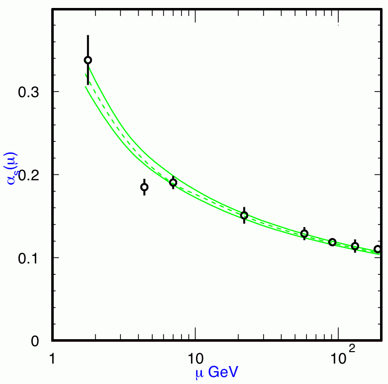
Figure 1.1: Summary of the values of $\alpha_{s}(\mu)$ at the energy scale of $\mu$ where they are measured. The lines show the central values and the $\pm 1\sigma$ limits of the average [1].

Asymptotic freedom can be explained by the self-interacting nature of the gluons. This self-interaction leads to a weak interaction between the quarks at small distances, and hence to asymptotic freedom. To understand confinement the strong interaction can be interpreted as a string, if two quarks are separated the energy density stored in the connecting string rises. At sufficient high densities the string breaks up forming a quark-antiquark pair, which are bound to the primary quarks. Consequently quarks can not be referred to as free particles at low energies.

1.1.3 Bound States

As described before the strong interaction binds the quarks into colorless states, the hadrons. Today two colorless bound states of quarks are well established: the mesons and the baryons. This two groups will be explained in more detail in the next two sections.
Recent measurements by Belle [12] and LHCb [13] seem to point to a new group of bound states, so called tetraquarks. But, since the nature of the observed tetraquark candidate $Z(4430)$ is not confirmed, this group of hadrons will be omitted.

Mesons

Mesons, consisting of a quark and an antiquark, pose the most simple combination of quarks into a colorless bound state. Meson ground states can be divided into pseudoscalar and vector mesons, depending on the spin orientation of the quark and antiquark. If the spins are aligned antiparallel $\uparrow\downarrow$ the meson is called a pseudoscalar meson, while a parallel $\uparrow\uparrow$ alignment is called a vector meson. Similar to atomic spectroscopy, excited states of mesons are possible by different values of the angular momentum $L$.
However, the picture, that a meson only consists of a quark and an antiquark, is too simple. Since the quarks are bound by gluons which are self-interacting and can fluctuate into quark-antiquark pairs the inner structure of a meson is much more complicated. The current model of the structure of a meson is that it consists of the valence quarks, the sea quarks and the sea gluons. The meson type is determined by the valence quarks alone.
The basic properties of the mesons relevant for this work are shown in Table 1.5. Here the width is an equivalent value to the lifetime for short-lived particles.

Baryons

Baryons, as second type of a bound state of quarks, consist of 3 valence quarks. The naming scheme relates to the isospin, as well as the quark content. For example baryons containing only two $u$ or $d$ quarks is called a $\mathchar 28931\relax$ (isospin $0$) or $\mathchar 28934\relax$ (isospin $1$). If the third quark is a charm or bottom quark it is given as index. For different mass states of the same quark content and isospin configuration the mass is given, e.g. $\mathchar 28934\relax_{c}(2520)$. Consisting of three valence quarks they follow the Fermi statistics. Well known baryons are the proton and the neutron as constituents of the nucleus. Table 1.5 shows the basic properties of the baryons relevant for this work.

Table 1.4: Mesons relevant for this work and their basic properties

Meson	quarks	mass in ${\mathrm{\,Me\kern-1.00006ptV\!/}c^{2}}$	lifetime	width $\Gamma$ in MeV
$\pi^{+}$	$u\overline{d}$	$139.57018\pm 0.00035$	$(2.6033\pm 0.0005)\cdot 10^{-8}$	$-$
$K^{+}$	$u\overline{s}$	$493.677\pm 0.016$	$(1.2385\pm 0.0024)\cdot 10^{-8}$	$-$
$B^{0}$	$d\overline{b}$	$5279.4\pm 0.5$	$(1.530\pm 0.009)\cdot 10^{-12}$	$-$
$\mathchar 28935\relax{(4S)}$	$b\overline{b}$	$10579.4\pm 1.2$	$-$	$20.5\pm 2.5$

Table 1.5: Baryons relevant for this work and their basic properties

Baryon	quarks	mass in ${\mathrm{\,Me\kern-1.00006ptV\!/}c^{2}}$	lifetime	width $\Gamma$ in MeV
$p$, $\overline{p}$	$uud$	$938.27203\pm 0.00008$	$>10^{31}$ years	$-$
$\mathchar 28931\relax_{c}^{+}$	$cud$	$2286.46\pm 0.14$	$(200\pm 6)\cdot 10^{-15}$s	$-$
$\mathchar 28934\relax_{c}(2455)^{++}$	$cuu$	$2453.98\pm 0.16$	$-$	$2.26\pm 0.25$
$\mathchar 28934\relax_{c}(2455)^{+}$	$cud$	$2452.9\pm 0.4$	$-$	$<4.6$
$\mathchar 28934\relax_{c}(2455)^{0}$	$cdd$	$2453.74\pm 0.16$	$-$	$2.16\pm 0.26$

Chapter 2 Baryonic $B$ decays

Baryons are the main constituent of the visible matter in our universe, but despite their large importance for our understanding of the universe little is known about their production mechanisms. A possibility is the production in decays of heavy mesons. Here, $B$ mesons are the first known mesons heavy enough to decay into a large variety of baryonic final states. In addition, decays into baryons make up a significant part of the overall branching fraction of $B$ mesons.

In the next sections a summary of the most striking results is given.

2.1 Multiplicity hierarchy

$B$-decays to baryons are not as well studied as mesonic decays. Previous measurements show a strong hierarchy of the branching fractions depending on the final state multiplicity, as shown in Table 2.1 for $B$ decays to a $\mathchar 28931\relax_{c}^{+}$ baryon and in Table 2.2 for decays to a charmed meson, accompanied by a baryon-antibaryon pair.

Table 2.1: Branching fraction results for $B\rightarrow\mathchar 28931\relax_{c}^{+}\bar{p}\;{\rm m}\cdot\pi$ with ${\rm m}=0,1,2,3$, ordered according to their multiplicity[7].

decay mode	${\cal B}\pm\sigma(10^{-4})$
$\bar{B}^{0}\rightarrow\mathchar 28931\relax_{c}^{+}\bar{p}$	$0.20\pm 0.04$
$\bar{B}^{0}\rightarrow\mathchar 28931\relax_{c}^{+}\bar{p}\pi^{0}$	$1.9\pm 0.5$
$B^{-}\rightarrow\mathchar 28931\relax_{c}^{+}\bar{p}\pi^{-}$	$2.8\pm 0.8$
$\bar{B}^{0}\rightarrow\mathchar 28931\relax_{c}^{+}\bar{p}\pi^{-}\pi^{+}$	$11.2\pm 3.2$
$B^{-}\rightarrow\mathchar 28931\relax_{c}^{+}\bar{p}\pi^{-}\pi^{-}\pi^{+}$	$22\pm 7$

For $B$ decays to a charmed baryon the branching fraction increases by an order of magnitude comparing the two-body decay $\bar{B}^{0}\rightarrow\mathchar 28931\relax_{c}^{+}\bar{p}$ with the three-body decays $\bar{B}^{0}\rightarrow\mathchar 28931\relax_{c}^{+}\bar{p}\pi^{0}$ and $B^{-}\rightarrow\mathchar 28931\relax_{c}^{+}\bar{p}\pi^{-}$. This increase is in contrast to the mesonic $B$ decays, where the three-body branching fraction is at the same order of magnitude as for the corresponding two-body mode. A possible explanation for the strong increase from the two-body to the three-body decay comes from the resonant substructure. The additional pion allows for $\mathchar 28934\relax_{c}$ and nucleon resonances, thus increasing the number of possible decay paths. Further, according to [14] the production of a two-body baryonic final state requires a hard gluon, introducing a strong suppression factor. Adding a light meson reduces the invariant mass of the remaining system, allowing for a soft gluon in the baryon production. For the decay into a charmed meson accompanied by a baryon-antibaryon pair the branching fraction reaches its maximum for multiplicities of four, as can be seen in Table 2.2.

Table 2.2: Branching fraction results for $B\rightarrow Dp\overline{p}\;{\rm m}\cdot\pi$ with ${\rm m}=0,1,2$ [6], ordered according to their multiplicity.

$B$ decay	${\cal B}\pm\sigma_{\rm stat}\pm\sigma_{\rm syst}$ $(10^{-4})$
$\kern 1.79993pt\overline{\kern-1.79993ptB}{}^{0}\rightarrow D^{0}p\overline{p}$	$1.02\pm 0.04\pm 0.06$
$\kern 1.79993pt\overline{\kern-1.79993ptB}{}^{0}\rightarrow D^{*0}p\overline{p}$	$0.97\pm 0.07\pm 0.09$
$\kern 1.79993pt\overline{\kern-1.79993ptB}{}^{0}\rightarrow D^{+}p\overline{p}\pi^{-}$	$3.32\pm 0.10\pm 0.29$
$\kern 1.79993pt\overline{\kern-1.79993ptB}{}^{0}\rightarrow D^{*+}p\overline{p}\pi^{-}$	$4.55\pm 0.16\pm 0.39$
$B^{-}\rightarrow D^{0}p\overline{p}\pi^{-}$	$3.72\pm 0.11\pm 0.25$
$B^{-}\rightarrow D^{*0}p\overline{p}\pi^{-}$	$3.73\pm 0.17\pm 0.27$
$\kern 1.79993pt\overline{\kern-1.79993ptB}{}^{0}\rightarrow D^{0}p\overline{p}\pi^{-}\pi^{+}$	$2.99\pm 0.21\pm 0.45$
$\kern 1.79993pt\overline{\kern-1.79993ptB}{}^{0}\rightarrow D^{*0}p\overline{p}\pi^{-}\pi^{+}$	$1.91\pm 0.36\pm 0.29$
$B^{-}\rightarrow D^{+}p\overline{p}\pi^{-}\pi^{-}$	$1.66\pm 0.13\pm 0.27$
$B^{-}\rightarrow D^{*+}p\overline{p}\pi^{-}\pi^{-}$	$1.86\pm 0.16\pm 0.19$

2.2 Threshold enhancement

A feature of baryonic $B$ decays observed quite frequently is an enhancement at low invariant baryon-antibaryon masses. Examples are shown in Fig. 2.1. Common to all the given examples is a deviation from a simple phasespace model at the invariant-mass threshold.

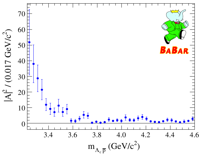
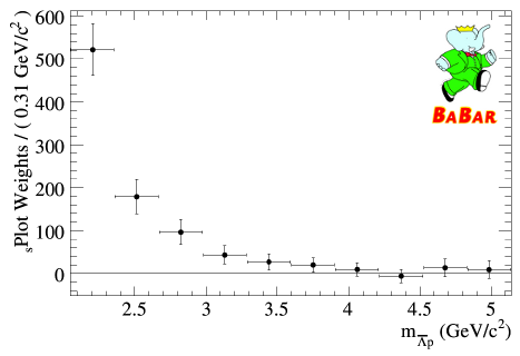
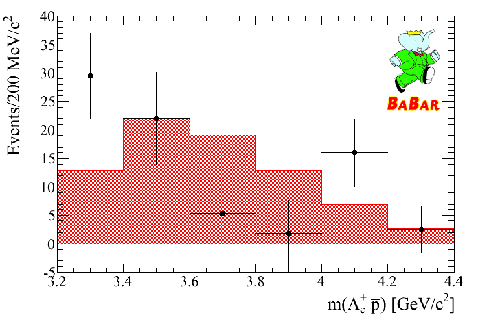
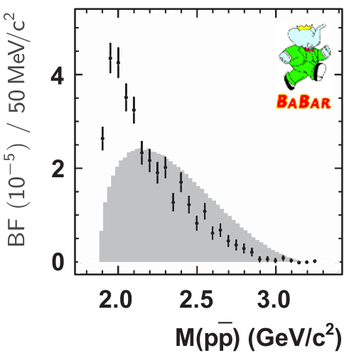
Figure 2.1: The invariant baryon antibaryon mass distributions for 2.1 $B^{-}\rightarrow\mathchar 28931\relax_{c}^{+}\overline{p}\pi^{-}$ [2], 2.1 $\kern 1.79993pt\overline{\kern-1.79993ptB}{}^{0}\rightarrow\mathchar 28931\relax\overline{p}\pi^{+}$ [3], 2.1 $\kern 1.79993pt\overline{\kern-1.79993ptB}{}^{0}\rightarrow\mathchar 28931\relax_{c}^{+}\overline{p}K^{-}\pi^{+}$ [4, 5] and 2.1 $\kern 1.79993pt\overline{\kern-1.79993ptB}{}^{0}\rightarrow D^{+}p\overline{p}\pi^{-}$ [6]. For the upper row the signal distribution was divided by the expectation from a simple phase space model. The lower row shows the signal distribution, with the phase space expectation represented as a histogram for $\kern 1.79993pt\overline{\kern-1.79993ptB}{}^{0}\rightarrow D^{+}p\overline{p}\pi^{-}$.

Explanations for this feature come from different sides. For decays of the type $B\rightarrow K+X$, with the fundamental subprocess $\overline{b}\rightarrow\overline{s}+g+g$ a strong contribution from a flavor-singlet penguin is expected. In terms of baryonic $B$ decays like $B^{+}\rightarrow p\overline{p}K^{+}$ a dominant contribution of a $p\overline{p}$ bound state with $J^{PC}=0^{\pm+}$ can provide a fair fraction of the observed final state [15].

For decays not dominated by flavor-singlet penguins a possible explanation for the threshold enhancement comes from the fragmentation into hadrons. If the baryons are neighbors in the fragmentation chain one expects their invariant mass to be low. A pole-model related rule of thumb, given in [16], is to check if the decay could proceed via an initial meson-meson or baryon-antibaryon configuration. In the first case one of the mesons decays into a baryon antibaryon pair, giving rise to the low mass enhancement. In the latter case no such enhancement is expected. This model is quite successful in explaining the results in $\kern 1.79993pt\overline{\kern-1.79993ptB}{}^{0}\rightarrow\mathchar 28931\relax_{c}^{+}\overline{p}\pi^{-}\pi^{+}$. In this analysis [16] an enhancement is seen for the resonant subdecay $\kern 1.79993pt\overline{\kern-1.79993ptB}{}^{0}\rightarrow\mathchar 28934\relax_{c}(2455)^{++}\overline{p}\pi^{-}$, while no enhancement is visible for $\kern 1.79993pt\overline{\kern-1.79993ptB}{}^{0}\rightarrow\mathchar 28934\relax_{c}(2455)^{0}\overline{p}\pi^{+}$. A comparison of phase space simulation and experimental data is shown in Fig. 2.2. Comparing the two distributions evidence for a low mass enhancement in $m(\mathchar 28934\relax_{c}(2455)^{++}\overline{p})$ is visible, while the low mass region in $m(\mathchar 28934\relax_{c}(2455)^{0}\overline{p})$ is unpopulated.

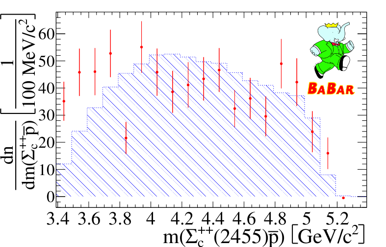
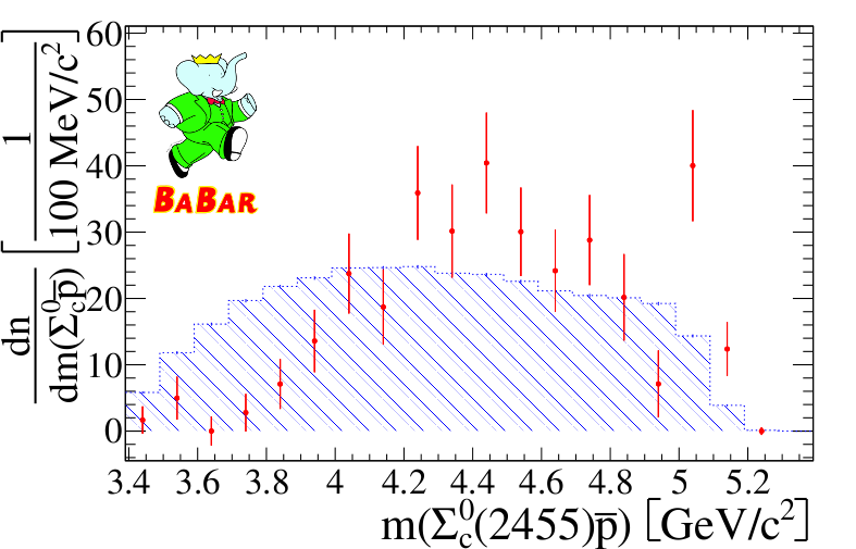
Figure 2.2: Comparison of phase space distributed signal Monte Carlo (histogram) with ${}_{s}P$lotted data (data points), 2.2 shows the invariant $\mathchar 28934\relax_{c}(2455)^{++}\overline{p}$ mass, and 2.2 the invariant $\mathchar 28934\relax_{c}(2455)^{0}\overline{p}$ mass.

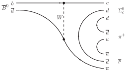
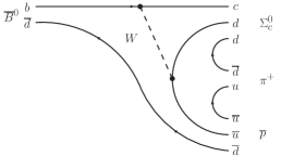
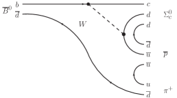
Figure 2.3: Comparison of the Feynman graphs responsible for the decay $\kern 1.79993pt\overline{\kern-1.79993ptB}{}^{0}\rightarrow\mathchar 28934\relax_{c}(2455)^{0}\overline{p}\pi^{+}$.

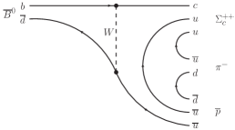
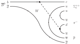
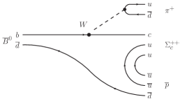
Figure 2.4: Comparison of the Feynman graphs responsible for the decay $\kern 1.79993pt\overline{\kern-1.79993ptB}{}^{0}\rightarrow\mathchar 28934\relax_{c}(2455)^{++}\overline{p}\pi^{-}$.

In [16] a simple model to explain the absence of an enhancement in $m(\mathchar 28934\relax_{c}(2455)^{0}\overline{p})$ is suggested. In this model the Feynman diagrams are categorized into two classes, according to their quark configuration after the weak decay.

• meson-meson configuration, i.e., before quark fragmentation, the quarks are arranged in two (virtual) mesons.

• diquark-diquark configuration, i.e., before quark fragmentation, the quarks are arranged in a diquark ($q_{1}q_{2}$) and an anti-diquark state.

In the meson-meson configuration one of the mesons fragments into a baryon anti-baryon pair, while the second meson carries away momentum, leading to a threshold enhancement. In the diquark-diquark configuration such an enhancement is not possible, since we already start from a baryon anti-baryon configuration. Comparing the Feynman graphs shown in Fig. 2.3 and 2.4 only the external graph in Fig. 2.4 is in the meson-meson configuration, which explains the absence of an enhancement for $\kern 1.79993pt\overline{\kern-1.79993ptB}{}^{0}\rightarrow\mathchar 28934\relax_{c}(2455)^{0}\overline{p}\pi^{+}$.

This approach seems to be valid for other $B$ meson decays into baryons as well, and is equivalent to the explanation via the fragmentation mechanism given in [15].

2.3 Semileptonic $B$ decays into baryons

Starting from the Feynman graphs shown in 2.3 and 2.4 we can assume that the threshold enhancement is caused by the external Feynman graph. In order to assess the relative influence of the external graph we have to investigate a decay, that can proceed only via an external graph. The ideal object for such a study is the semileptonic decay $B^{-}\rightarrow\mathchar 28931\relax_{c}^{+}\overline{p}\ell^{-}\overline{\nu}_{\ell}$, with $\ell^{-}=(e^{-},\mu^{-})$ and $\overline{\nu}_{\ell}=(\overline{\nu}_{e},\overline{\nu}_{\mu})$ (Charge conjugation is implied throughout this work). The corresponding Feynman graph is shown in Fig. 2.5.

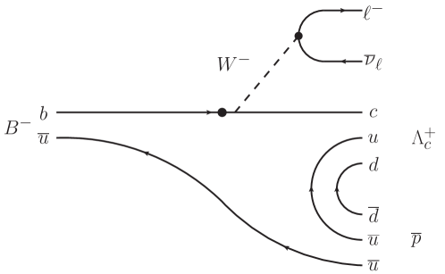
Figure 2.5: Feynman graph for the decay $B^{-}\rightarrow\mathchar 28931\relax_{c}^{+}\overline{p}\ell^{-}\overline{\nu}_{\ell}$.

Up to now, there are only upper limits for its relative strength available. The CLEO collaboration showed that the ratio of $B\rightarrow\mathchar 28931\relax_{c}^{+}Xe^{-}\overline{\nu}_{e}$ to $B\rightarrow\mathchar 28931\relax_{c}^{+}X$ is smaller than $5\%$ at $90\%\;{\rm C.L.}$[17]. But this result has two caveats. First, the lepton momentum is required to be greater than $0.6{\mathrm{\,Ge\kern-1.00006ptV\!/}c}$, which reduces background from fake and secondary electrons, but the signal efficiency as well. Second, uncorrelated $\kern 1.79993pt\overline{\kern-1.79993ptB}{}\rightarrow\kern 1.99997pt\overline{\kern-1.99997pt\mathchar 28931\relax\kern 0.50003pt}\kern-0.50003pt{}^{-}_{c}X$ events pose a large source of systematic uncertainty. To circumvent these caveats BABAR uses a tagged approach, by reconstructing a $B$ meson in a hadronic mode and looking for the signal in its recoil [18]. With this approach BABAR determines the before mentioned ratio to be

$$\frac{{\cal B}(\kern 1.79993pt\overline{\kern-1.79993ptB}{}\rightarrow\mathchar 28931\relax_{c}^{+}X\ell^{-}\overline{\nu}_{\ell})}{{\cal B}(\kern 1.79993pt\overline{\kern-1.79993ptB}{}\rightarrow\mathchar 28931\relax_{c}^{+}X)}<3.5\%$$ (2.1)

at the $90\%$ confidence level.

The first direct measurement of a semileptonic baryonic $B$ decay is a recent publication by the Belle collaboration [19]. Like the previously mentioned BABAR measurement they use a tagged approach, and found evidence for the decay $B^{-}\rightarrow p\overline{p}\ell^{-}\overline{\nu}_{\ell}$. For this measurement Belle studied $615$ exclusive hadronic decays of charged $B$ mesons. Paired with the large dataset of $772$ million $B{\kern-1.60004pt\kern 1.79993pt\overline{\kern-1.79993ptB}{}}$ pairs they measured a branching fraction of

$${\cal B}(B^{-}\rightarrow p\overline{p}\ell^{-}\overline{\nu}_{\ell})=(5.8^{+2.4}_{-2.1}({\rm stat})\pm 0.9({\rm syst}))\times 10^{-6}$$ (2.2)

with a significance of $3.2\sigma$. The corresponding upper limit at $90\%{\rm C.L.}$ is

$${\cal B}(B^{-}\rightarrow p\overline{p}\ell^{-}\overline{\nu}_{\ell})<9.6\times 10^{-4}.$$ (2.3)

Starting from the measurement of $B^{-}\rightarrow p\overline{p}\ell^{-}\overline{\nu}_{\ell}$ a rough estimate of the branching fraction for $B^{-}\rightarrow\mathchar 28931\relax_{c}^{+}\overline{p}\ell^{-}\overline{\nu}_{\ell}$ can be obtained. Neglecting phase space differences, the only difference is the CKM matrix element in the $b$ quark decay. For the former $|V_{ub}|$ has to be considered, while the latter depends on $|V_{cb}|$. The ratio $|V_{cb}/V_{ub}|$ equals $9.9$ [7], and hence we can expect

$${\cal B}(B^{-}\rightarrow\mathchar 28931\relax_{c}^{+}\overline{p}\ell^{-}\overline{\nu}_{\ell})\approx(5.7\pm 2.9)\times 10^{-4}.$$ (2.4)

Another approach to obtain a branching fraction estimate is the fully hadronic decay $B^{-}\rightarrow\mathchar 28931\relax_{c}^{+}\overline{p}\pi^{-}$ which is measured to be $(2.8\pm 0.8)\times 10^{-4}$[7]. Neglecting any influence of internal $W$ emission diagrams we can obtain a branching fraction by assuming

$$\frac{{\cal B}(B^{-}\rightarrow\mathchar 28931\relax_{c}^{+}\overline{p}\ell^{-}\overline{\nu}_{\ell})}{{\cal B}(B^{-}\rightarrow\mathchar 28931\relax_{c}^{+}\overline{p}\pi^{-})}=\frac{{\cal B}(\tau^{-}\rightarrow\ell^{-}\overline{\nu}_{\ell}\nu_{\tau})}{{\cal B}(\tau^{-}\rightarrow\pi^{-}\nu_{\tau})}.$$ (2.5)

${\cal B}(\tau^{-}\rightarrow\pi^{-}\nu_{\tau})$ is measured to $(10.83\pm 0.06)\%$, ${\cal B}(\tau^{-}\rightarrow e^{-}\overline{\nu}_{e}\nu_{\tau})$ to $(17.83\pm 0.04)\%$, ${\cal B}(\tau^{-}\rightarrow\mu^{-}\overline{\nu}_{\mu}\nu_{\tau})$ to $(17.41\pm 0.04)\%$ [7]. Neglecting the small difference between the latter two the ratio is roughly $1.8$, which leads to

$${\cal B}(B^{-}\rightarrow\mathchar 28931\relax_{c}^{+}\overline{p}\ell^{-}\overline{\nu}_{\ell})\approx(4.7\pm 1.3)\times 10^{-4}.$$ (2.6)

An estimate for the semileptonic branching fraction could be obtained in the isospin analysis of $\kern 1.79993pt\overline{\kern-1.79993ptB}{}^{0}\rightarrow\mathchar 28931\relax_{c}^{+}\overline{p}\pi^{0}$ and $\kern 1.79993pt\overline{\kern-1.79993ptB}{}^{0}\rightarrow\mathchar 28931\relax_{c}^{+}\overline{p}\eta$ [20]. Based on isospin relations the author predicts the relative strength of the external Feynman graph in $B^{-}\rightarrow\mathchar 28931\relax_{c}^{+}\overline{p}\pi^{-}$ of $(0.20\pm 0.45)\times 10^{-4}$. Combined with the ratio of $\tau$ decays this leads to a $90\%$ confidence level upper limit for the semileptonic decay of

$${\cal B}(\kern 1.79993pt\overline{\kern-1.79993ptB}{}^{0}\rightarrow\mathchar 28931\relax_{c}^{+}\overline{p}e^{-}\overline{\nu}_{e})<1.4\times 10^{-4}.$$ (2.7)

This result shows a slight tension with the predictions given in eq. (2.4) and (2.6). But given the limitations of these predictions the isospin prediction might be the most reliable one.

Chapter 3 The BABAR experiment

The BABAR experiment, operated from 1999 to 2008, was designed and built to perform a systematic study of $C\!P$-asymmetries in the decays of neutral $B$-mesons. Furthermore, BABAR allowed a sensitive measurement of the CKM matrix element $|V_{ub}|$ and observations of rare $D$, $B$ and $\tau$-decays. Together these results are capable of putting constraints on fundamental parameters of the Standard Model. In addition a wide spectrum of physics topics, like baryonic $B$-decays or charm- and tau-physics, could be studied with the BABAR detector. For the investigation of $B$-mesons BABAR was operated on the energy of the $\mathchar 28935\relax{(4S)}$ ($10.58\mathrm{\,Ge\kern-1.00006ptV}$) resonance, which decays into a $B\kern 1.79993pt\overline{\kern-1.79993ptB}{}$ pair with a probability of more than $96\%$[7]. The data set collected on this resonance is the starting point for the presented analysis.
The experimental setup, shown in Fig. 3.1, is described in detail in the next sections, following the description given in [10].

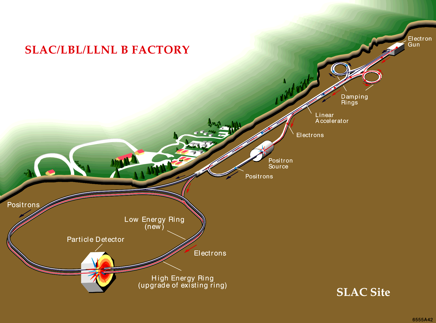
Figure 3.1: A schematic view of the SLAC site with the $e^{+}e^{-}$ accelerator and the BABAR detector

3.1 The $e^{+}e^{-}$ accelerator

Electrons and positrons were accelerated in the $3.2{\rm\,km}$ long Linac up to energies of several $\mathrm{\,Ge\kern-1.00006ptV}$ and injected into the PEP-II storage rings, where they were brought to collision inside the BABAR detector.
Inside PEP-II, electrons were stored in the high energy ring (HER) with an energy of $9\mathrm{\,Ge\kern-1.00006ptV}$, while the positrons were stored in the low energy ring (LER) with an energy of approx. $3.1\mathrm{\,Ge\kern-1.00006ptV}$. These energies meet the requirement of a center-of-mass energy $\sqrt{s}$ equal to the mass of the $\mathchar 28935\relax{(4S)}$ resonance, which decays into $B\kern 1.79993pt\overline{\kern-1.79993ptB}{}$ pairs, half of the time into a $B^{0}{\kern-1.60004pt\kern 1.79993pt\overline{\kern-1.79993ptB}{}^{0}}$- and the other half into a $B^{+}{\kern-1.60004ptB^{-}}$-pair.
The cross-sections for the different reactions possible in the $e^{+}e^{-}$ collision at $\sqrt{s}=10.58\mathrm{\,Ge\kern-1.00006ptV}$ can be seen in table 3.1. Bhabha-scattering ($e^{+}e^{-}\rightarrow e^{+}e^{-}$) has by far the highest cross-section, while the other reactions are near $1{\rm\,nb}$. Consequently, in most of the collisions, no $b\overline{b}$-pair is produced.
The unique chance BABAR offered were the asymmetric beam energies, leading to a boost of the center-of-mass system into the direction of the electron beam. The boost is crucial for studies of $C\!P$ asymmetries, by allowing a measurement of the difference in the decay times of the two $B$ mesons. Therefore, the decay vertices of the $B$-mesons have to be measured. The decay time difference can now be estimated by measuring the distance between the two vertices.

Table 3.1: Production cross-sections at $\sqrt{s}=10.58\mathrm{\,Ge\kern-1.00006ptV}$. The $e^{+}e^{-}$ cross-section is the effective cross-section within the experimental acceptance [8].

$e^{+}e^{-}\rightarrow$	cross-section (${\rm\,nb}$)
$b\overline{b}$	$1.05$
$c\overline{c}$	$1.30$
$s\overline{s}$	$0.35$
$u\overline{u}$	$1.39$
$d\overline{d}$	$0.35$
$\tau^{+}\tau^{-}$	$0.94$
$\mu^{+}\mu^{-}$	$1.16$
$e^{+}e^{-}$	$\approx 40$

3.2 The BABAR detector

The foremost requirement on the detector was a maximal acceptance in the center-of-mass system. Due to the asymmetric beam energies the decay products were boosted in the forward direction of the laboratory frame. Thus, an asymmetric detector was necessary to optimize the detector acceptance. Furthermore, an excellent vertex resolution, as well as a good discrimination between $e$, $\mu$, $\pi$, $K$, and $p$ over a wide kinematic range and the capability to detect and identify neutral particles were necessary.
BABAR has been designed to meet all of these requirements. Picture 3.2 shows a schematic view of the BABAR detector. The detector was arranged cylindrically around the beam pipe and consisted from the center outwards of the following subsystems:

• The Silicon Vertex Tracker (SVT), was providing precise position information on charged tracks, is the only tracking device for very low-energy charged particles,

• the Drift Chamber (DCH) provided the main momentum measurement for charged particles, and helped in particle identification by measuring the energy loss of traversing particles,

• the Detector of Internally Reflected Cherenkov light (DIRC), responsible for the identification of charged hadrons,

• the Electromagnetic Calorimeter (EMC), was providing information about neutral particles as well as a good electron identification,

• the superconducting coil, was providing a $1.5\rm T$ solenoidal magnetic field for the momentum measurement in the DCH, and

• the Instrumented Flux Return (IFR) was used for muon and neutral hadron identification.

The different parts will be explained in the following section. A more detailed description of the detector can be found in [8], [21] and [22].

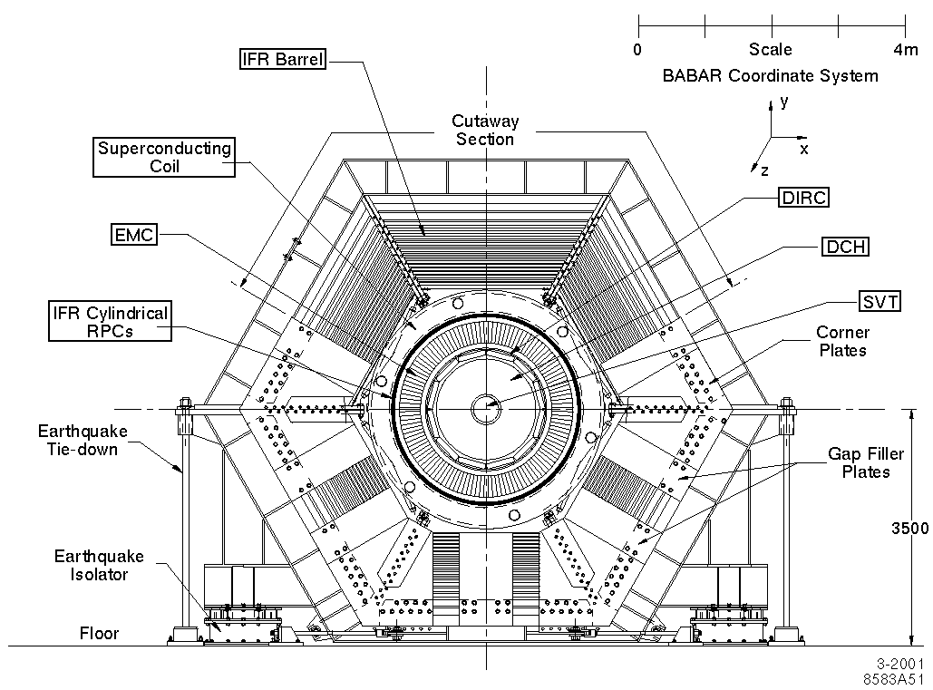
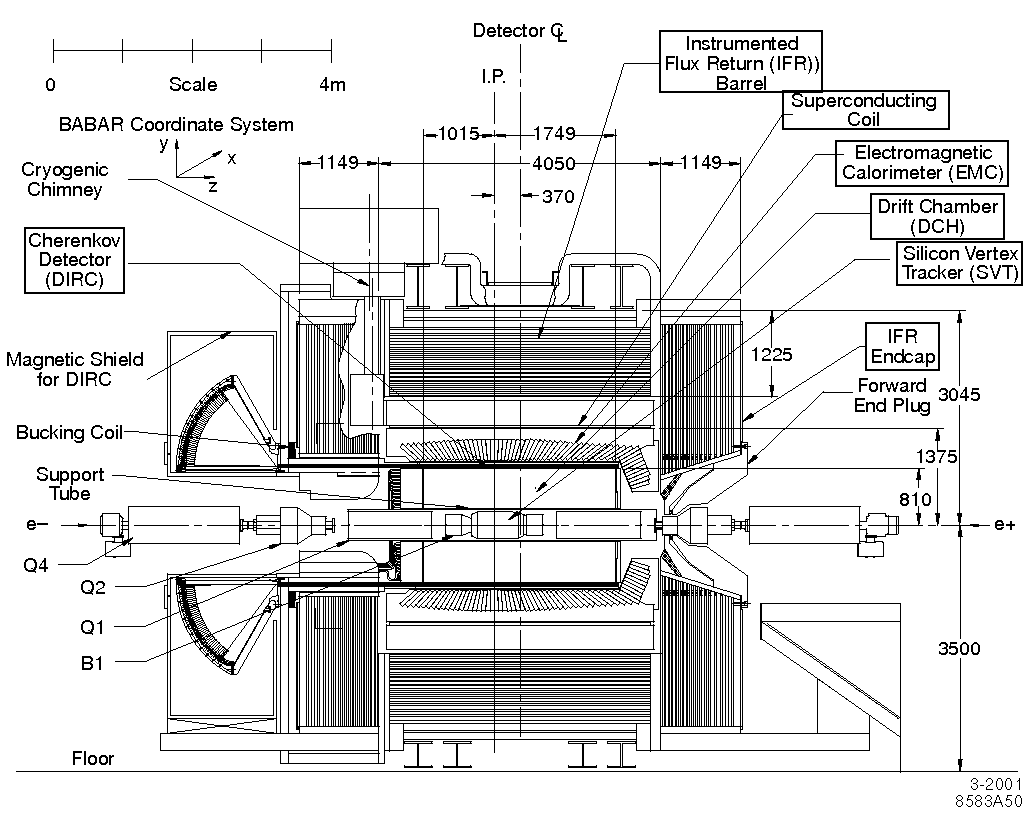
Figure 3.2: The BABAR detector: In the upper right corner the BABAR coordinate system is shown, $z$ is the direction of the electron beam, $y$ points upwards while $x$ points horizontally away from the center of the PEP-II ring. 3.2 shows the detector end view (looking into the direction of the HER beam), while 3.2 shows a longitudinal cut of the detector.

3.2.1 Silicon Vertex Tracker

The Silicon Vertex Tracker (SVT) was the detector component with the smallest distance to the interaction point (IP). Consequently, it was the first component providing information on the flight path (track) of the particles emerging from the interaction point. Furthermore, it was the only source of information for low momentum particles that did not reach the drift chamber due to their deflection caused by the magnetic field.
The SVT, shown in Fig. 3.3, was located inside a $4.5{\rm\,m}$ long support tube. It consisted of five concentric cylindrical layers of double-sided silicon detectors. These five rings had radii of $3.3{\rm\,cm}$ up to $14.6{\rm\,cm}$. If a charged particle crossed the SVT it generated electron-hole pairs leading to a signal. Due to the segmentation of the SVT, the signals in the different segments provided information about the path of the particle. Besides, the SVT also provided information for the particle identification of charged particles with momenta less than $700{\mathrm{\,Me\kern-1.00006ptV\!/}c}$ by measuring the rate of energy loss $\mathrm{d}E/\mathrm{d}x$ [23]. Figure 3.4 shows the energy loss per travelled path against the momentum of the particle for different particles in the SVT.
The three rings closest to the IP delivered data about the position and the angle of a track for the track reconstruction with a spatial resolution of $10-15{\,\mu\rm m}$ [24]. The two outer rings had a resolution of $30-40{\,\mu\rm m}$ [24] and were important for the measurement of the momentum of particles with a small transversal momentum as well as for the separation of geometrically close tracks.

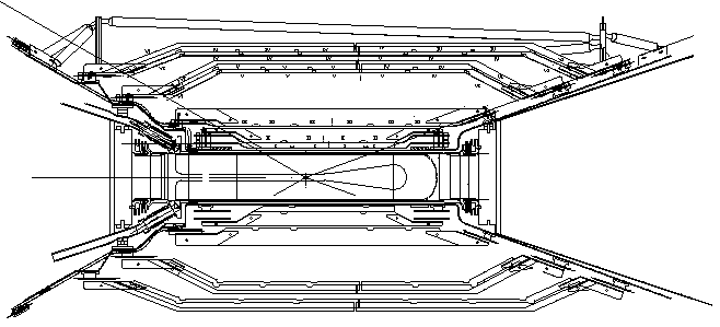
Figure 3.3: Longitudinal view of the SVT

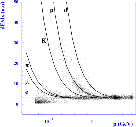
Figure 3.4: Energy loss per travelled path versus momentum in the SVT for different particles. $e$ - electron, $\mu$ - muon, $K$ - kaon, $p$ - proton, $d$ - deuteron

3.2.2 Drift Chamber

The drift chamber (DCH) was the main tracking device of the BABAR detector. It measured at least 40 space coordinates per track in the central region, ensuring a high reconstruction efficiency for tracks with transverse momentum greater than $100{\mathrm{\,Me\kern-1.00006ptV\!/}c}$. Further, the drift chamber contributed to the particle identification. Therefore, the rate of energy loss was measured, this rate is characteristical for the different types of particles. Figure 3.5 shows the rate of energy loss versus momentum.
The drift chamber was a $280{\rm\,cm}$ long cylinder, with an inner radius of $23.6{\rm\,cm}$ and an outer radius of $80.9{\rm\,cm}$. It consisted of $7104$ hexagonal cells, which were formed by $6$ field wires in the corners of the hexagon and a sense wire in the center of the cell. The cells were arranged in $10$ superlayers of $4$ layers each. Axial (A) and stereo (U,V) superlayers alternate as it can be seen in Fig. 3.6. This led to a $z-$coordinate resolution of $700{\,\mu\rm m}$ [25].
If a particle crossed the drift chamber it ionized the gas mixture ($80\%$ Helium, $20\%$ Isobutane) inside the chamber. The generated ions and electrons drifted towards the field wires or to the sense wires, respectively, due to a difference in the voltage of $1960\rm V$ between the sense and field wires. The generated signal could be used for tracking as well as for particle identification by the measurement of $\mathrm{d}E/\mathrm{d}x$. Figure 3.7 shows the spatial resolution of the drift cells.

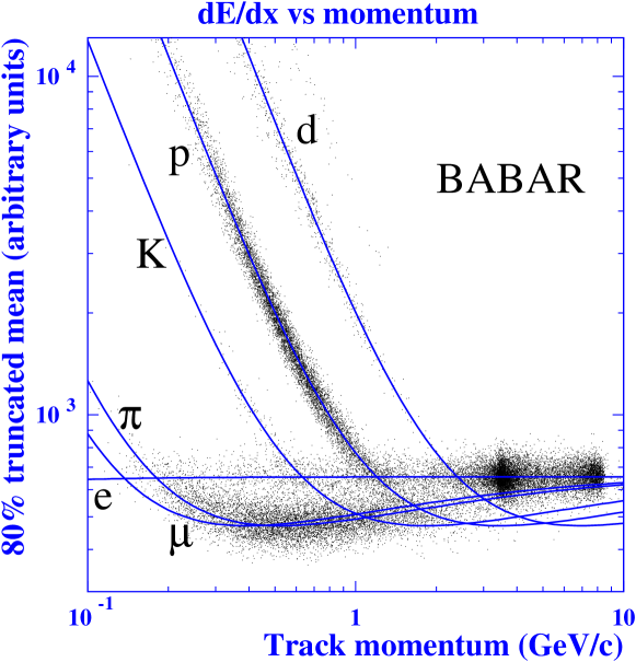
Figure 3.5: energy loss per travelled path versus momentum in the DCH for different particles ($e$ - electron, $\mu$ - muon, $K$ - kaon, $p$ - proton, $d$ - deuteron)

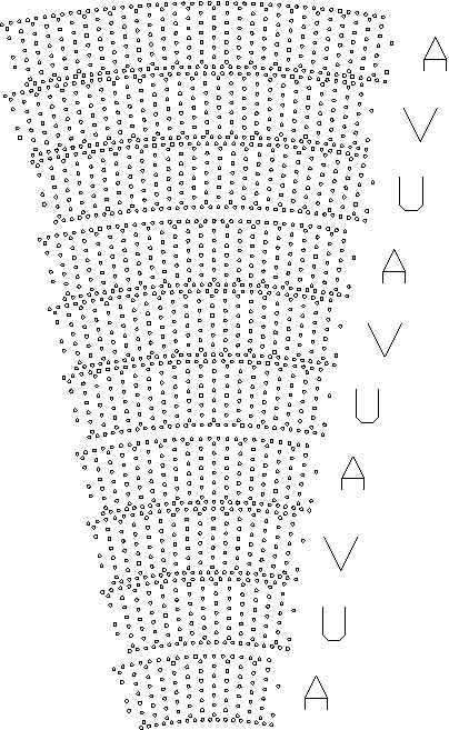
Figure 3.6: Cell layout in the BABAR drift chamber

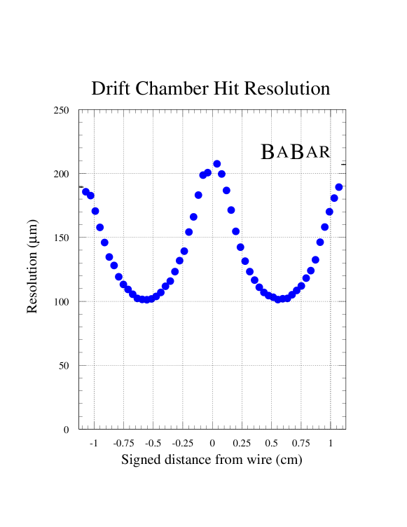
Figure 3.7: Spatial resolution of the drift cells

3.2.3 Superconducting Solenoid

Although the superconducting solenoid, together with the instrumented flux return, was the outermost detector component its function was closely related to the drift chamber. The solenoid, a superconducting coil, created a magnetic field of $1.5$ Tesla inside the drift chamber leading to a deflection of the track of a charged particle. This deflection was used to measure the charge as well as the momentum of a charged particle with a transverse momentum resolution of $\sigma(p_{T})/p_{T}\approx 0.45\%+0.13\%\cdot p_{T}$ [25].

3.2.4 Detector for internally reflected Cherenkov light

The Detector for internally reflected Cherenkov light (DIRC) was capable of identifying pions and kaons with momenta greater than $0.7{\mathrm{\,Ge\kern-1.00006ptV\!/}c}$ as well as protons with momenta between $1.3{\mathrm{\,Ge\kern-1.00006ptV\!/}c}$ and $4{\mathrm{\,Ge\kern-1.00006ptV\!/}c}$. This was complementary to the drift chamber, which could identify particles with lower momenta.

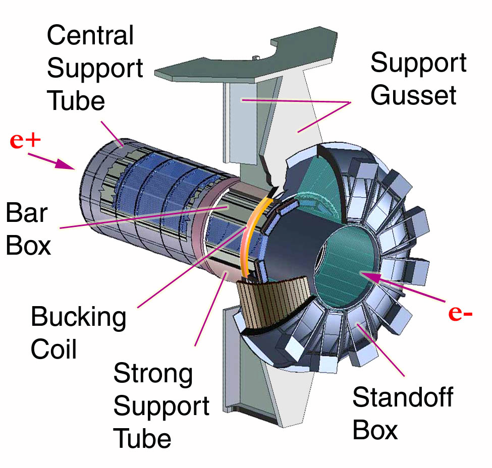
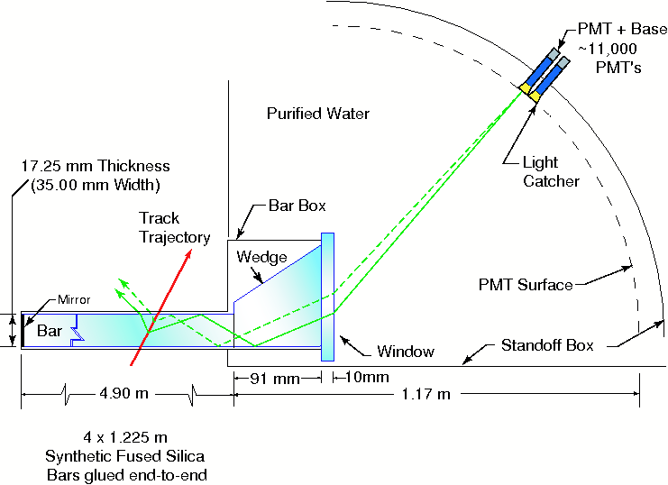
Figure 3.8: Fig. 3.8 shows a schematic view of the DIRC, the bar box containing the quartz bars and the standoff box are clearly visible. Fig. 3.8 illustrates the mode of operation of the DIRC. The emitted Cherenkov light is guided by total internal reflection to the standoff box where the Cherenkov angle is measured with the help of photomultiplier tubes.

Fig. 3.8 shows a schematic view of the DIRC. It consisted of $144$ bars of synthetic quartz with a refractive index of $n\approx 1.474$ surrounding the drift chamber. If a particle crossed these bars with a velocity larger than the speed of light inside the quartz it produced Cherenkov light. The Cherenkov photons were emitted at an angle $\theta_{c}$ relatively to the direction of the particle. This angle depends on the mass and momentum of the particle.

$$\cos\theta_{c}=\frac{1}{\beta n}=\frac{\sqrt{1+\left(\frac{m}{p}\right)^{2}}}{n}$$ (3.1)

Inside the bars the Cherenkov photons were reflected many times until they entered the standoff box at the rear side of the detector. This box was filled with about $6000$ liters of purified water and was equipped with nearly $11000$ photo multiplier tubes to detect the Cherenkov angle. Fig. 3.9 shows the discrimination power of the Cherenkov angle. The angular resolution of the DIRC for a single photon was $7\rm\,mrad$ [26].

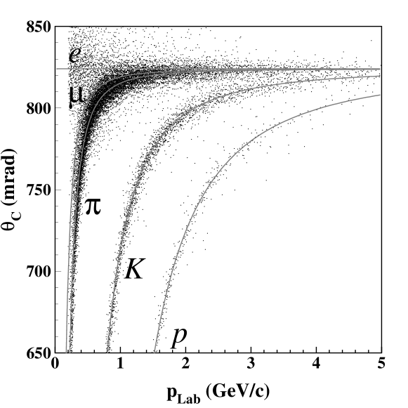
Figure 3.9: Cherenkov angle against momentum for different particles

3.2.5 Electromagnetic Calorimeter

The BABAR electromagnetic calorimeter (EMC), as shown in Fig. 3.10, was a hollow cylinder surrounding the drift chamber. The calorimeter barrel consisted of $5760$ thallium-doped CsI crystals arranged in $48$ rings of $120$ crystals, while the End Cap was composed of $820$ crystals.

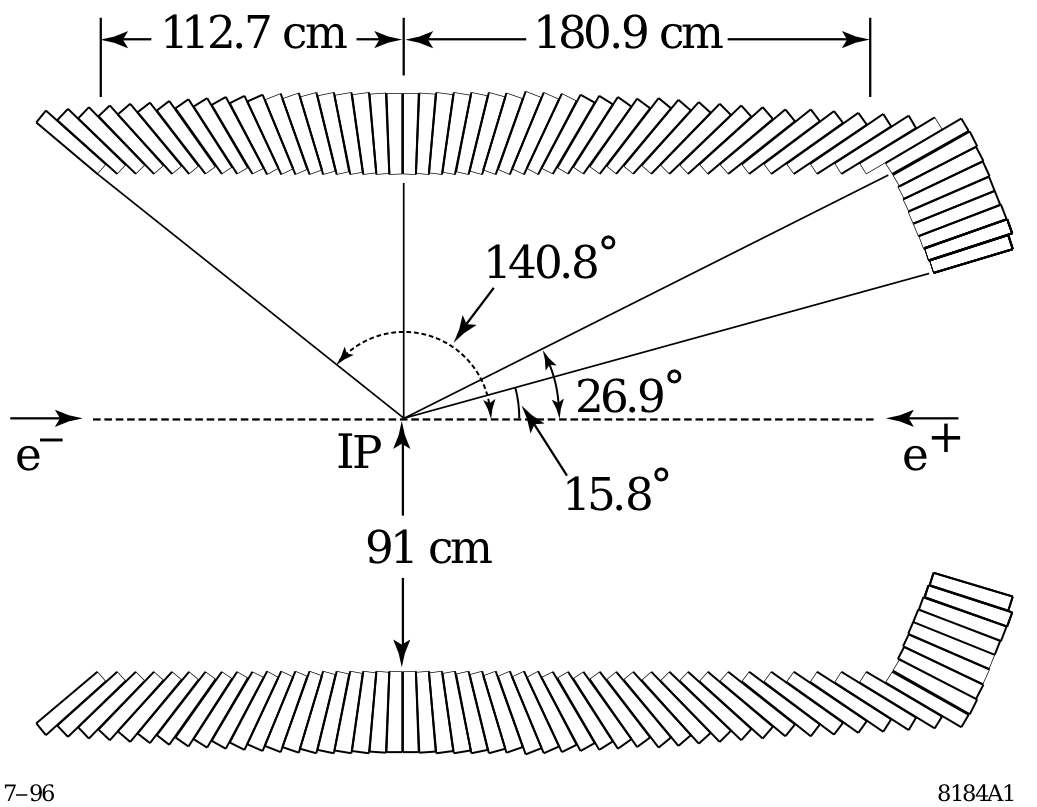
Figure 3.10: schematic view of the EMC, showing the calorimeter barrel and the forward End Cap.

The calorimeter was designed for excellent efficiency as well as good energy ($\sigma_{E}/E$) and angular resolution of the energy range $20\mathrm{\,Me\kern-1.00006ptV}$ to $9\mathrm{\,Ge\kern-1.00006ptV}$. A detailed study [27] gave

$$\frac{\sigma_{E}}{E} =\frac{(2.30\pm 0.03\pm 0.3)\%}{\sqrt[4]{E(\mathrm{\,Ge\kern-1.00006ptV})}}\oplus(1.35\pm 0.08\pm 0.2)\%$$ (3.2)

$$\sigma_{\theta} =\sigma_{\phi}=\frac{(4.16\pm 0.04)\rm\,mrad}{\sqrt{E(\mathrm{\,Ge\kern-1.00006ptV})}}.$$ (3.3)

Here, the $\oplus$ denotes a quadratic summation. Due to the asymmetric design the calorimeter covered a solid angle of $-0.775\leq\cos\theta\leq 0.962$ in the laboratory frame and $-0.916\leq\cos\theta\leq 0.895$ in the center-of-mass frame [8].
High energetic photons entering a crystal were converted into $e^{+}e^{-}$ pairs by interacting with the crystal. The created electrons and positrons emitted bremsstrahlung photons which could convert into $e^{+}e^{-}$ pairs again. An electromagnetic shower developed. The generated photons could be absorbed by the scintillator material leading to an excitation of the crystal atoms. When the atom returned into its groundstate it emitted the absorbed energy as light. This light could be detected by photo diodes glued to the rear end of the crystals. Here the amount of measured light was proportional to the energy lost inside the crystals by a particle crossing the EMC.
In addition to the detection of photons the calorimeter was an important detector component for the discrimination between electrons and other particles. Details on the electron identification with the help of the EMC are given in section 3.3.3.

3.2.6 Instrumented Flux Return

The outermost layer of the BABAR detector was the instrumented flux return (IFR). Its main purpose as a detector component was the identification of muons as well as neutral hadrons like the $K_{L}^{0}$ mesons. Consisting of a central part (Barrel) and two End doors the IFR covered a solid angle range down to $300\rm\,mrad$ in the forward, and $400\rm\,mrad$ in the backward direction [8]. In the initial setup the IFR was instrumented with $806$ Resistive Plate Chambers (RPCs), arranged in $19$ layers in the barrel and $18$ layers in the End Caps. Already in the first year of data taking the RPCs showed serious aging problems and had to be replaced by second generation RPCs and Limited Streamer Tubes (LSTs). The final configuration of the IFR consisted of $12$ layers of LSTs in the barrel and 16 layers of second generation RPCs in the forward End Cap. In the backward End Cap the original RPCs were retained. During the upgrade to LSTs the remaining flux return slots were filled with brass absorber plates, and some external steel plates were added. Thereby the pion rejection ability of the muon identification algorithm, described in section 3.3.3, was improved [28]. A sketch of the final IFR configuration can be seen in Fig. 3.11.

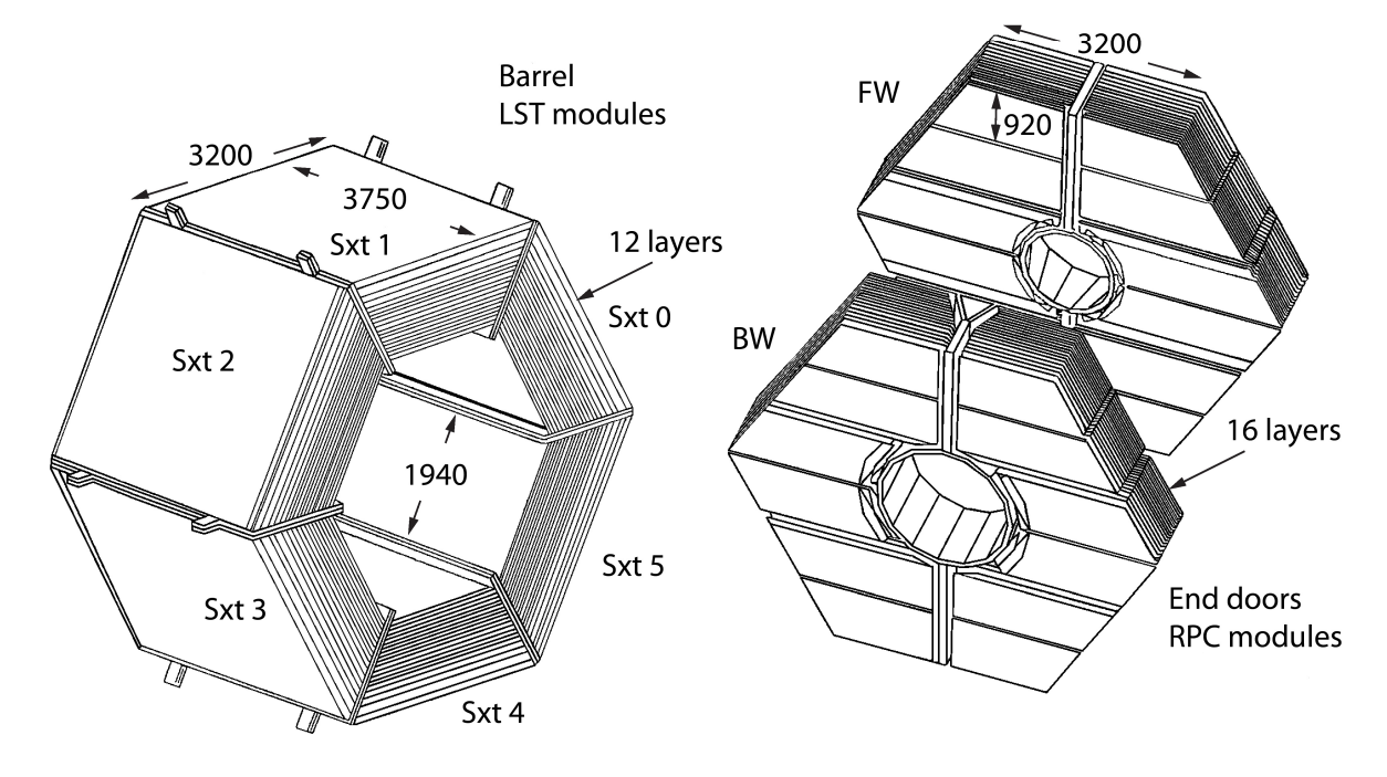
Figure 3.11: Final layout of the IFR with barrel sextants, forward (FW) and backward (BW) end caps, the dimensions are given in ${\rm\,mm}$.

3.2.7 Trigger

The BABAR trigger consisted of two levels: a hardware level (called Level 1) and a software level (called Level 3) and had to decide which events observed by the BABAR detector were interesting enough to be kept and recorded for later analysis.
The Level 1 trigger system consisted of four subsystems: the charged particle trigger (DCH trigger - DCT), the neutral particle trigger (EMC trigger - EMT), the cosmic trigger (IFR trigger - IFT) and the Global Level Trigger (GLT).
The DCT and EMT received information from the Drift Chamber and the Calorimeter, respectively, processed it and sent the condensed information to the Global Trigger. This trigger tried to match the angular locations of calorimeter towers and drift chamber tracks and generated Level 1 trigger signal, which were passed to the Level 3 trigger. In addition to the information from the DCT and EMT the Global Trigger also uses IFT information to trigger on cosmic rays and $\mu$-pair events.
After the Level 1 trigger the Level 3 trigger, operating on an online farm, analyzed the event data from the DCH and EMC in conjunction with the Level 1 trigger information for further background reduction. Besides the physics filter this trigger stage also performed Bhabha veto and the selection of calibration events as well as critical online monitoring tasks [29].

3.3 Event reconstruction

The events that have been selected to be kept were passed to the reconstruction software which reconstructed the tracks in an event and assigned particle hypotheses to the tracks.
During the reconstruction neutral and charged particles had to be considered separately. Charged particles interacted with every detector component and left a track inside the detector that could be reconstructed. In contrast, neutral particles only interacted with the EMC and the IFR. Consequently, their reconstruction relied on information delivered by these two detector components like their shower shape in the EMC and the energy deposit in the detector.

3.3.1 Neutrals

All neutrals in the BABAR framework are based on CalorNeutral, a standard list created during online production. This list contains all EMC clusters that are not assigned to any track in the event. For all these entries the photon mass-hypothesis is applied.

Based on CalorNeutral BABAR uses two photon lists, namely GoodPhotonLoose and GoodPhotonDefault [30]. The first one contains all candidates from CalorNeutral satisfying the following criteria:

• Minimum raw energy of $0.03\mathrm{\,Ge\kern-1.00006ptV}$

• Maximum Lateral Moment $LAT$ of $0.8$.

The GoodPhotonDefault list contains all candidates from GoodPhotonLoose with a minimum raw energy of $0.1\mathrm{\,Ge\kern-1.00006ptV}$.

3.3.2 Track reconstruction

For charged particles a multi-step track reconstruction takes place. The first step is to search for track points in both tracking devices (SVT and DCH) separately. Due to the multi-layer design of the SVT and DCH it is possible to reconstruct the path a particle took inside these detector components, therefore a curve is fitted to the track points in the respective subdetector. Afterwards the reconstruction program tries to assign partial tracks inside the SVT and in the DCH to each other. After a successful assignment the combined track is fitted again to provide a good momentum measurement.
The least stringent requirement for an accepted track is a successful reconstruction of the track as well as a successful momentum measurement. A track fulfilling these conditions is assigned to the ChargedTracks list under a pion hypothesis.
Table 3.2 shows the requirements for the tracking lists used at BABAR, as they can be found in [31]. The different selection criteria shown in table 3.2 are:

• transverse momentum $p_{t}$ $\left[{\mathrm{\,Ge\kern-1.00006ptV\!/}c}\right]$

• momentum $p$ $\left[{\mathrm{\,Ge\kern-1.00006ptV\!/}c}\right]$

• distance of closest approach (DOCA) to the $z$-axis in the $xy$-plane $d_{0}$ $\left[cm\right]$

• $z$-coordinate of the point of closest approach $z_{0}$ $\left[cm\right]$

• fit probability $P(\chi^{2})$

Table 3.2: Tracking lists used at BABAR and the selection criteria for these lists

tracking list	$p_{t}$	$p$	$|d_{0}|$	$|z_{0}|$	$P$
ChargedTracks	-	-	-	-	$>0$
GoodTracksVeryLoose	-	-	$<1.5$	$<2.5$	$>0$
GoodTracksLoose	$>0.05$	$<10$	$<1.5$	$<2.5$	$>0$

For the latter neutrino reconstruction we have to rely on ChargedTracks since identified $V_{0}$ tracks, including $K_{s}$, $\mathchar 28931\relax$ and converted $\gamma$ are not included in the more stringent lists GoodTracksVeryLoose and GoodTracksLoose.

3.3.3 Charged Particle Identification

The identification of charged particles is crucial for many analyses performed at BABAR. For a high quality of the identification all BABAR subdetectors contributed in a complementary way to charged particle identification. The SVT and DCH provides $\mathrm{d}E/\mathrm{d}x$ measurements, the DIRC provides a velocity measurement, the EMC discriminates electrons, muons and hadrons according to their energy deposit and their shower shape while the IFR characterizes muons and hadrons according to their different interaction pattern.

Electron identification with the EMC

For the electron identification with the calorimeter we have to distinguish between two methods.

1. Electron identification using $E/p$

2. Electron identification using the shower shape

For the first method the ratio $E/p$ is measured, where $E$ is the energy of a shower in the calorimeter, and $p$ is the measured three-momentum of the corresponding charged track. When an electron enters the calorimeter it produces an electromagnetic shower, depositing its energy in the calorimeter. Thus, the ratio $E/p$ is expected to be close to unity for an electron. In contrast muons and charged hadrons deposit only a fraction of their energy in the calorimeter, leading to smaller values of $E/p$. In addition to the good separation of electrons this method can also be used for a discrimination of muons against hadrons. While muons, as single minimum-ionizing particles, have a well-defined peak in the $E/p$ distribution, hadrons have additional tails at higher $E/p$ values. A caveat of the $E/p$ method is that hadrons interact electromagnetically as well as hadronically with the calorimeter. In the latter case they initiate a hadronic shower, depositing a large fraction of their energy in the calorimeter. Since the resulting $E/p$ values are rather large a discrimination against electrons by $E/p$ alone is difficult. An improvement of the electron identification can be achieved by using the different shower shape for electrons and hadrons. While electrons deposit most of their energy in two or three crystals hadronic showers are more extended. A quantity reflecting this difference is the lateral moment $LAT$

$$LAT=\frac{\sum_{i=3}^{N}E_{i}r_{i}^{2}}{\sum_{i=3}^{N}E_{i}r_{i}^{2}+E_{1}r_{0}^{2}+E_{2}r_{0}^{2}}.$$ (3.4)

Here, the energies $E_{i}$ are ordered according to their value ($E_{1}>E_{2}>\ldots>E_{N}$), with $N$ being the number of crystals associated with the shower. $r_{i}$ and $\phi_{i}$ are the polar coordinates of the crystal in the plane perpendicular to the line pointing from the interaction point to the center of the shower. $r_{0}$ is the average distance between two crystals ($\approx 5{\rm\,cm}$). Since the summation omits the two crystals with the highest energy deposit this quantity is expected to be small for electromagnetic showers. An even better discrimination between electrons and hadrons is achieved by including information about the azimuthal distribution of the shower. In general electromagnetic showers are expected to be isotropic in $\phi$, while hadronic showers are far more irregular in $\phi$.

Muon identification with the IFR

The first step for muon identification with the IFR is the track reconstruction. Due to the low occupancy this is an uncritical task, since only a tiny fraction of tracks overlap each other. First, tracks are reconstructed in each sector using a clustering algorithm. In the second step the clusters in different sectors are merged, using the extrapolation of the charged tracks measured by the tracking systems (SVT and DCH) into the IFR. Such composite clusters are considered as candidates for muons or charged hadrons.
For the muon identification the algorithm has to decide, whether the detected track has been produced by a muon or a pion. The other hadron candidates, kaons and protons, are identified by the other particle identification sub-systems since they show a similar signature like the pion in the IFR. For the discrimination of muons against charged hadrons different IFR variables are used, e.g. the number of strips in IFR cluster, the number of measured interaction lengths, and the continuity of IFR hits in the 3-D IFR cluster [8, 32].

BDT selectors

For muons we apply the BDT selector, which is based on a Bagged Decision Tree (also Bootstrap Aggregating Decision Tree). A decision tree splits an $n$ dimensional input set (with $M$ entries) into rectangular subsets (nodes), where for each split all variables are considered and the split that leads to the largest increase in the figure of merit (e.g. the muon efficiency) is selected. This split is repeated recursively for each of the resulting nodes. The recursion ends when the number of entries in a node hits a pre-defined minimum $m$, or if the figure of merit doesn’t change significantly. If the majority of entries in this node are signal entries this node is classified as a signal node, otherwise it is a background node. To enhance the reliability and reduce the variance of this procedure many trees are trained on bootstraped replicas of the training set. The bootstraped replica is obtained by sampling with replacement from the original training set, until the size of the replica equals the size of the original training set. For an improvement of the performance compared to a single tree the classifier used has to be sensitive to small changes in the training set. This is obtained by setting a small value for $m$, and thus overtraining the trees. While each tree has a poor predictive power the final vote, a majority vote of all trained trees, has a high predictive power [33]. The major goal of the BDT selectors is to provide a constant muon efficiency over time, momentum $\vec{p}$ and polar angle $\theta$. While the last two are easy to understand the constant efficiency over time incorporates the aging of the detector components for the muon identification, as well as upgrades of the IFR. The muon efficiencies for the different PID lists can be found in Tab. 3.3. Details on the BDT input variables and performance can be found in [34].

Table 3.3: The target efficiencies for the muon BDT lists. While in the first four lists a constant muon efficiency was targeted, the following four lists aimed at a constant pion mis-ID. The last two lists are specially designed for muons with momenta in the range $0.3$ to $0.7{\mathrm{\,Ge\kern-1.00006ptV\!/}c}$.

List name	muon eff.	pion mis-ID
muBDTVeryLoose	$90.0\%$	variable
muBDTLoose	$80.0\%$	variable
muBDTTight	$70.0\%$	variable
muBDTVeryTight	$60.0\%$	variable
muBDTVeryLooseFakeRate	variable	$5.0\%$
muBDTLooseFakeRate	variable	$3.0\%$
muBDTTightFakeRate	variable	$2.0\%$
muBDTVeryTightFakeRate	variable	$1.2\%$
muBDTLoPLoose	$70.0\%$	variable
muBDTLoPTight	$60.0\%$	variable

KM selectors

The KM lists are based on Error Correcting Output Code, that combines multiple binary classifiers to form a multiclass classifier. Here, the binary classifiers are trained differently. In the case of the KM selectors seven Bootstrap Aggregate Decision Trees $t_{i}$ were trained according to Table 3.4.

Table 3.4: The used indicator matrix in the KM selector. Each entry indicates whether the given training sample should be treated as signal (1) or background (-1).

Class	$t_{0}$	$t_{1}$	$t_{2}$	$t_{3}$	$t_{4}$	$t_{5}$	$t_{6}$
$K$	$1$	$1$	$1$	$1$	$1$	$1$	$1$
$\pi$	$-1$	$1$	$-1$	$1$	$-1$	$1$	$-1$
$p$	$1$	$-1$	$-1$	$1$	$1$	$-1$	$-1$
$e$	$1$	$1$	$1$	$-1$	$-1$	$-1$	$-1$

For the classification of a given track each classifier $t_{i}$ is asked to give an output between $-1$ and $1$, resulting in a string of seven real values between $-1$ and $1$. This string is then compared to the individual codeword for class $k$. For a kaon the codeword is the first row in Table 3.4, for a $\pi$ the second and so on. The comparison is here done by calculating the generalized Hamming distance $H_{k}$, the sum of squared differences, to the codeword for each class $k$. The track is then assigned to the class with the lowest Hamming distance. In order to obtain multiple tightness levels we can use the distance $H_{k}$ itself as well as ratios of distances. For a kaon list we can use $H_{K}$, $H_{\pi}/H_{K}$, $H_{p}/H_{K}$ and $H_{e}/H_{K}$. For the other particle classes we use the analogue ratios. This method allows us to control the probability for a given class as well as the misidentification rate. More details on these selectors, especially on the chosen input variables for the seven classifiers can be found in [35].

For high flexibility special selectors for the pre-selection of recorded data, were introduced. These CombinedSuperLoose selectors combine the least restrictive selectors for a given particle type to allow the user to switch to his selector of choice in the event reconstruction.

Chapter 4 Software and Datasets

4.1 Software

For the reconstruction of the decay we use the following packages inside the BABAR framework

• analysis-52

• BetaMiniUser V00-04-05

• PDT V00-07-00

• workdir V00-04-21

The event selection and background reduction uses the data analysis package ROOT [36] and iPython [37] with SciPy [38].

In the background reduction we apply a random forest, provided by SciPy, to distinguish between signal and background candidates. A random forest is a modification of the bagging method, as described in sect. 3.3.3, where a large collection of trees is build, and the response is averaged over all trees. The benefit is that one can use models with a small predictive power, thus unbiased, for classification in this method [39]. For bagged trees the bias is the same as for the individual tree. In consequence the only improvement can be obtained in terms of the variance of the average

$$\rho\sigma^{2}+\frac{1-\rho}{B}\sigma^{2},$$ (4.1)

which depends on the pairwise tree correlation $\rho$, the individual tree variance $\sigma^{2}$ and the number of trees $B$. While the second term vanishes for large $B$ the first term stays unchanged.

The idea behind the random forest algorithm is to reduce the correlation $\rho$ without increasing the variance $\sigma^{2}$. This is achieved by a random selection of the input variables during the tree-growing process. In the following we will concentrate on a bootstrapped dataset. For bootstrapping the dataset $\bf Z$, containing $N$ candidates described by $p$ variables, is divided into $B$ datasets. For the division we draw from $\bf Z$ randomly with replacement $B$ datasets $Z_{1},\ldots,Z_{B}$ containing the same number of events $N$ as the original dataset $\bf Z$.

The general algorithm of the training of a random forest is shown in algorithm 4.1.

Algorithm 4.1 Training of a random forest [39]

1. for $b=1$ to $B$:

   1. Draw a bootstrap sample $Z_{b}$ of size $N$ from the training data

   2. Grow a tree $T_{b}$ to $Z_{b}$, by recursively repeating the following for each terminal node, until minimum node size $n_{\rm min}$ (number of candidates) is reached

      1. select $m$ variables at random from the $p$ variables

      2. pick the best variable/split-point among the $m$

      3. split the node into two daughter nodes

2. output the ensemble of trees $\{T_{B}\}^{B}_{1}$.

The split is done by selecting the variable most suitable to discriminate signal from background, and dividing the dataset into two hemispheres. Subsequently each hemisphere is handed over to one of the two daughter nodes. Finally, each node $l$ represents a subregion $R_{l}$, with $N_{l}$ observations of the whole input data set. The proportion of class $k$ in this region is thus given by

$$\hat{p}_{lk}=\frac{1}{N_{l}}\sum_{x_{i}\in R_{l}}I(y_{i}=k),$$ (4.2)

where $x_{i}$ denotes the candidate to be classified and $y_{i}$ the class of $x_{i}$. The function $I(y_{i}=k)$ returns $1$ if $y_{i}=k$ and $\mathrm{𝟎}$ otherwise. For final nodes all observations in the node are classified as the class with the highest value for $\hat{p}_{lk}$.

In the application phase each tree returns a classification prediction $\hat{C}_{b}(x)$. The resulting classification prediction from the random forest is then the majority vote of $\hat{C}_{b}(x)$, with $b=1\ldots B$.

The relevant tuning variables here are the number of trees $B$, the minimal node size $n_{\rm min}$ and the number of randomly to choose variables $m$.

4.2 Datasets

Data taking on the $\mathchar 28935\relax{(4S)}$ resonance at BABAR took place in six run periods between February 2000 and August 2007. The data set used in this analysis comprises the complete data collected by BABAR on the $\mathchar 28935\relax{(4S)}$ resonance, with an integrated luminosity of

$$\mathcal{L}_{\rm OnPeak}=(424\,000\pm 1900_{\rm syst})\mbox{\,pb}^{-1}.$$ (4.3)

This corresponds to a total number of $B\kern 1.79993pt\overline{\kern-1.79993ptB}{}$ pairs of

$$N_{B\kern 1.25995pt\overline{\kern-1.25995ptB}{}}=470\,960\,000\pm 116\,000_{\rm stat}\pm 2\,826\,000_{\rm syst}.$$ (4.4)

In addition to the OnPeak data set various Monte Carlo modes have been used to study background behavior and for the training of the random forest. The used background modes are listed in Table 4.1.

Table 4.1: Monte Carlo modes used for background studies. Given are their SP number in BABAR bookkeeping and the contained number of events.

mode	SP number	number of events
$e^{+}e^{-}\rightarrow q\overline{q}$, $q=u,d,s$	998	$2\,190\,254\,000$
$e^{+}e^{-}\rightarrow c\overline{c}$	1005	$1\,127\,360\,000$
$e^{+}e^{-}\rightarrow B^{+}{\kern-1.60004ptB^{-}}$	1235	$707\,282\,000$
$e^{+}e^{-}\rightarrow B^{0}{\kern-1.60004pt\kern 1.79993pt\overline{\kern-1.79993ptB}{}^{0}}$	1237	$716\,219\,000$

For the signal description we chose two different approaches, a simple phase space model, and a simulation reproducing the threshold enhancement seen in various baryonic $B$-decays (see sect. 2.2). For the first one, the Phase Space (PS) model, we simulate a $B$-meson decaying directly into the final state particles $\mathchar 28931\relax_{c}^{+}$, $\overline{p}$, $\ell^{-}$ and $\overline{\nu}_{\ell}$. Here, the four-momenta are distributed uniformly in phase space. This model is intended for studies of the systematic uncertainties arising from the chosen decay model. For the second model, the Weak Interaction (WI) model, we assume that the hadronic form factor is given by the decay $B^{-}\rightarrow\mathchar 28931\relax_{c}^{+}\overline{p}\pi^{-}$. For this purpose we defined a meson pole $M$, decaying into the baryon anti-baryon pair $\mathchar 28931\relax_{c}^{+}\overline{p}$.

$$B^{-}\rightarrow M \ell^{-}\overline{\nu}_{\ell}$$

$$M\rightarrow \mathchar 28931\relax_{c}^{+}\overline{p}$$

$$\mathchar 28931\relax_{c}^{+} \rightarrow pK^{-}\pi^{+}$$ (4.5)

Mass and width of the $M$ are chosen to reflect the properties of the enhancement known from other decay modes, especially from $B^{-}\rightarrow\mathchar 28931\relax_{c}^{+}\overline{p}\pi^{-}$[2]. The mass is chosen in such a way that the mass peak is slightly above threshold, at $3.225{\mathrm{\,Ge\kern-1.00006ptV\!/}c^{2}}$ and the width is derived from the $m(\mathchar 28931\relax_{c}^{+}\overline{p})$ distribution in [2] (Fig. 4.1) to be $200{\mathrm{\,Me\kern-1.00006ptV\!/}c^{2}}$.

Figure 4.1: Invariant $\mathchar 28931\relax_{c}^{+}\overline{p}$ mass for the decay $B^{-}\rightarrow\mathchar 28931\relax_{c}^{+}\overline{p}\pi^{-}$, divided by the expectation from a phase space model.

The semi-leptonic decay $B^{-}\rightarrow M\ell^{-}\overline{\nu}_{\ell}$ is modeled according to the weak matrix element

$$|{\cal M}|^{2}=(p_{B}p_{\nu})(p_{\ell}p_{M}),$$ (4.6)

under the assumption that the spectator system collapses into one particle. The subsequent decay $M\rightarrow\mathchar 28931\relax_{c}^{+}\overline{p}$ is simulated according to phase space.

The WI model is expected to give a more realistic momentum and energy spectrum for the charged lepton and the neutrino as well as a more realistic $m(\mathchar 28931\relax_{c}^{+}\overline{p})$ distribution. Fig. 4.2, 4.3 show a comparison of energy and momentum for both models on generator level in the center-of-mass frame.

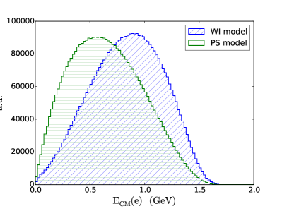
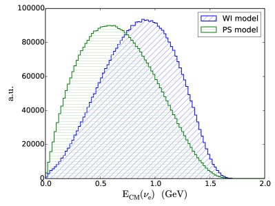
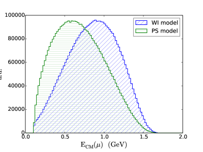
Figure 4.2: Comparison of the charged lepton (left) and neutrino (right) energy for the PS and WI model, scaled to the same integral. The first row shows the electron, and the last row the muon channel.

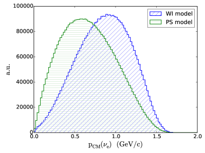
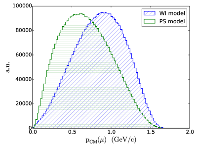
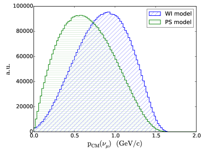
Figure 4.3: Comparison of the charged lepton (left) and neutrino (right) momentum for the PS and WI model, scaled to the same integral. The first row shows the electron, and the last row the muon channel.

For the invariant $\mathchar 28931\relax_{c}^{+}\overline{p}$ mass a comparison on generator level, as shown in Fig. 4.4, shows a peak above threshold for the Weak Interaction model, while the Phase Space model shows a broad spectrum.

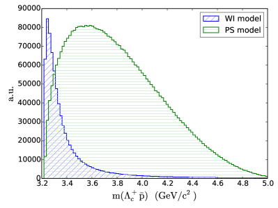
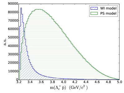
Figure 4.4: Comparison of the invariant $\mathchar 28931\relax_{c}\ \overline{p}$ mass for the PS and WI model, scaled to the same height. Fig. 4.4 shows the electron, and 4.4 the muon channel.

All signal modes, generated using EvtGen [40] for the decay simulation and GEANT [41] for modelling the detector response, are given in Table 4.2.

Table 4.2: Monte Carlo modes used for signal studies and the number of generated events. The upper half shows the direct decay of the $B$ into the final state, described by a simple phase space model. The lower half gives the modes reproducing the threshold enhancement.

mode	number of signal events
$B^{-}\rightarrow\mathchar 28931\relax_{c}^{+}\overline{p}e^{-}\overline{\nu}_{e}$	$4\,180\,000$
$B^{-}\rightarrow\mathchar 28931\relax_{c}^{+}\overline{p}\mu^{-}\overline{\nu}_{\mu}$	$4\,220\,000$
$\kern 1.79993pt\overline{\kern-1.79993ptB}{}^{0}\rightarrow\mathchar 28931\relax_{c}^{+}\overline{p}\pi^{+}e^{-}\overline{\nu}_{e}$	$4\,230\,000$
$\kern 1.79993pt\overline{\kern-1.79993ptB}{}^{0}\rightarrow\mathchar 28931\relax_{c}^{+}\overline{p}\pi^{+}\mu^{-}\overline{\nu}_{\mu}$	$4\,260\,000$
$B^{-}\rightarrow Me^{-}\overline{\nu}_{e}$, $M\rightarrow\mathchar 28931\relax_{c}^{+}\overline{p}$	$2\,867\,841$
$B^{-}\rightarrow M\mu^{-}\overline{\nu}_{\mu}$, $M\rightarrow\mathchar 28931\relax_{c}^{+}\overline{p}$	$3\,098\,301$

Chapter 5 Event reconstruction

Subject of the present work is the study of the two baryonic $B$-decay modes $B^{-}\rightarrow\mathchar 28931\relax_{c}^{+}\overline{p}e^{-}\overline{\nu}_{e}$ and $B^{-}\rightarrow\mathchar 28931\relax_{c}^{+}\overline{p}\mu^{-}\overline{\nu}_{\mu}$. The reconstruction of the $B$ candidate is done in four separate steps. In the first step a $\mathchar 28931\relax_{c}^{+}$ candidate is reconstructed which is used in the second step to reconstruct the visible part of the $B$ decay, namely $\mathchar 28931\relax_{c}^{+}\overline{p}\ell^{-}$, henceforth denoted as $Y$ system.

$$B^{-}\rightarrow\underbrace{\mathchar 28931\relax_{c}^{+}\overline{p}\ell^{-}}_{\displaystyle Y}\overline{\nu}_{\ell}$$ (5.1)

The third step is the reconstruction of the neutrino as missing energy and momentum in the event. In the last step the reconstructed neutrino is combined with the $Y$ to form a $B$ candidate.

5.1 $\mathchar 28931\relax_{c}^{+}$ reconstruction

The $\mathchar 28931\relax_{c}^{+}$ is reconstructed in its dominant decay mode $\mathchar 28931\relax_{c}^{+}\rightarrow pK^{-}\pi^{+}$, which has a branching fraction of $(5.0\pm 1.3)\%$ [7]. The $p$, $K^{-}$ and $\pi^{+}$ candidates are combined and fitted to a common vertex to form a $\mathchar 28931\relax_{c}^{+}$ candidate. A $\mathchar 28931\relax_{c}^{+}$ candidate is accepted if the vertex fit with the TreeFitter algorithm is successful and the invariant mass of the candidate is within the interval from $2.235$ to $2.332{\mathrm{\,Ge\kern-1.00006ptV\!/}c^{2}}$. The particle identification (PID) requirements for the three input particles are listed in Table 5.1.

particle	PID list
$p$	pCombinedSuperLoose
$K^{-}$	KCombinedSuperLoose
$\pi^{+}$	piCombinedSuperLoose

Table 5.1: PID lists used for the $\mathchar 28931\relax_{c}^{+}$ reconstruction.

5.1.1 $\mathchar 28931\relax_{c}^{+}$ mass constraint

In order to improve the resolution of the reconstructed events a mass constraint on the nominal $\mathchar 28931\relax_{c}^{+}$ mass is applied prior to the $Y$ reconstruction (see section 5.2). The standard mass value for the constraint is the one used for the Monte Carlo production which is $2.2849{\mathrm{\,Ge\kern-1.00006ptV\!/}c^{2}}$. We use this value in the reconstruction of Monte Carlo events. For data a precise measurement of the $\mathchar 28931\relax_{c}^{+}$ mass shows a momentum dependence of the mass mean value as well as a bias introduced by the SVT material density used in the reconstruction [42]. To determine the optimal mass value for the constraint we perform an extended maximum-likelihood fit to the $m(pK^{-}\pi^{+})$ distribution in data. As fit function we use a second order Chebychev polynomial for background and a Gaussian for the signal description. The fit can be seen in Fig. 5.1, while the fit parameters are given in Table 5.2.

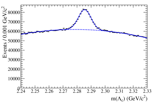
Figure 5.1: Fitted $\mathchar 28931\relax_{c}^{+}$ mass distribution for OnPeak data.

Parameter	fitted value
$N_{\rm bkg}$	$5348820\pm 2969$
$N_{\rm sig}$	$237499\pm 1924$
$\mu$	$2.285446\pm 0.000029$
$\sigma$	$0.004489\pm 0.000034$
$b_{1}$	$-0.033696\pm 0.00076$
$b_{2}$	$-0.059378\pm 0.00095$

Table 5.2: Fit parameters for the fit to the $\mathchar 28931\relax_{c}^{+}$ mass in OnPeak data.

We decide to constrain the $\mathchar 28931\relax_{c}^{+}$ mass in data to $2.2854{\mathrm{\,Ge\kern-1.00006ptV\!/}c^{2}}$.

5.2 Reconstruction of the visible decay products

For the reconstruction of the $Y$ system the previously reconstructed $\mathchar 28931\relax_{c}^{+}$ candidate is combined with an $\overline{p}$, and an $e^{-}$ or $\mu^{-}$ candidate. The particle identification at this stage is based on the PID lists given in Table 5.3. To make sure that the lepton lies within the acceptance region of the SVT, DCH and EMC (excluding the not well calibrated part of the EMC in the backward region) the polar angle $\theta_{\ell}$ of the lepton has to be within $0.41\ldots 2.37\,{\rm rad}$. The resulting $Y$ candidate is discarded if a fit of the daughters to a common vertex is not successful. To select those $Y$ candidates with a four-momentum $p_{Y}$ consistent with a $B^{-}\rightarrow Y\nu\rightarrow\mathchar 28931\relax_{c}^{+}\overline{p}\ell\nu$ decay we use the angle between the $B$ meson and the $Y$ candidate $\theta_{BY}$ (defined in the center-of-mass system).

In semileptonic $B$ decays the four-momentum of the neutrino can be expressed as

$$p_{\nu}^{2}=0=(p_{B}-p_{Y})^{2}=M_{B}^{2}+M_{Y}^{2}-2(E_{B}E_{Y}-|\vec{p}_{B}||\vec{p}_{Y}|\cos\theta_{BY}).$$ (5.2)

Here, $E_{B}$ and $|\vec{p}_{B}|$ can be derived from the center-of-mass energy. For $M_{B}$ the world average value can be used. Under the assumption that we have a perfectly reconstructed semileptonic decay, we can determine $\cos\theta_{BY}$

$$\cos\theta_{BY}=\frac{2E_{B}E_{Y}-M_{B}^{2}-M_{Y}^{2}}{2|\vec{p}_{B}||\vec{p}_{Y}|}.$$ (5.3)

To retain only physical values of $\cos\theta_{BY}$ and to suppress background from wrongly reconstructed $Y$ candidates we require $|\cos\theta_{BY}|<1.2$, allowing for resolution effects in the reconstruction of this quantity. A comparison of OnPeak data and the WI signal Monte Carlo is shown in Fig. 5.2. For light hadronic final states we would expect a strong enhancement at positive values for signal events, while background events (which make up most of the OnPeak data) should show no such peak. This strong difference is smeared out when considering a heavy final state like in the case of $B^{-}\rightarrow\mathchar 28931\relax_{c}^{+}\overline{p}\ell^{-}\overline{\nu}_{\ell}$ where the $B$ direction is dominated by the $\mathchar 28931\relax_{c}^{+}\overline{p}$ system. In consequence the peak for signal Monte Carlo is broadened, while background events tend to prefer values near $+1$ as well.

Table 5.3: Particle ID lists used for the $Y$ reconstruction.

particle	PID list
$p$	pCombinedSuperLoose
$e^{-}$	eCombinedLoose
$\mu^{-}$	muCombinedVeryLooseFakeRate

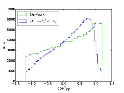
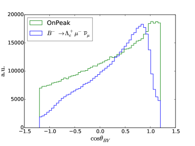
Figure 5.2: Comparison of $\cos\theta_{BY}$ in OnPeak data and WI signal Monte Carlo for the electron 5.2 and the muon 5.2 channel. For both plots a subset of all reconstructed candidates was used, requiring the $m_{\rm ES}$, $\Delta E$ and $m(\mathchar 28931\relax_{c}^{+})$ cuts described later on.

5.3 Neutrino reconstruction

Under the assumption that there are no undetected particles in the event the neutrino can be reconstructed as missing energy and missing momentum of the event. In an $e^{+}e^{-}$ experiment like BABAR the energy and momentum of the CM system are well known for each interaction. To determine the missing energy and momentum in principle all seen particles ($E_{i}$,$\vec{p}_{i}$) have to be subtracted from the CM system ($E_{CM}$, $\vec{p}_{CM}$). For neutral particles, mainly photons, the GoodPhotonLoose list is used. For charged particles the ChargedTracks list has to be used since the higher quality list GoodTracksVeryLoose does not contain neutral particles that are converted into charged particles inside the detector, e.g. $\gamma\rightarrow e^{+}e^{-}$, or $K_{s}^{0}\rightarrow\pi^{+}\pi^{-}$.

$$(E_{\nu},\vec{p}_{\nu})=(E_{\rm miss},\vec{p}_{\rm miss})=(E_{CM},\vec{p}_{CM})-(\sum_{i}E_{i},\sum_{i}\vec{p}_{i})$$ (5.4)

The major problem is to assign the correct particle hypothesis to the charged tracks. In the ChargedTracks list the default hypothesis for each track is the pion hypothesis, i.e. the mass for each track is set to the pion mass. In order to circumvent this potential bias we assign more realistic particle hypotheses to the tracks for the neutrino reconstruction. Therefore each element of ChargedTracks is compared in a well defined order with stringent particle identification lists, given in Table 5.4. If the track is not used inside the $\mathchar 28931\relax_{c}^{+}$ or $Y$ the according particle hypothesis is applied to the track, otherwise the same hypothesis as in the $\mathchar 28931\relax_{c}^{+}$ or $Y$ has to be used. The comparison with the particle identification lists is done in the following order:

1. if track $\in$ electron list $\rightarrow$ electron PID is assigned

2. else if track $\in$ kaon list $\rightarrow$ kaon PID is assigned

3. else if track $\in$ muon list $\rightarrow$ muon PID is assigned

4. else if track $\in$ proton list $\rightarrow$ proton PID is assigned

5. else pion PID is assigned.

Table 5.4: Particle ID lists used for the neutrino reconstruction.

particle type	PID list
electron	eKMTight
kaon	KKMTight
muon	muBDTVeryLoose
proton	pKMTight

5.4 $B$ reconstruction

Subsequently the reconstructed $Y$ and $\nu$ candidate are combined to a $B$ candidate. Kinematic consistency of the candidate with a $B$ decay is checked using two variables, the beam energy substituted mass, $m_{\rm ES}$, and the difference between the reconstructed and expected energy of the candidate, $\Delta E$. They are defined as

$$\Delta E =E_{B}^{*}-\sqrt{s}/2$$ (5.5)

$$m_{\rm ES} =\sqrt{\frac{(s/2+\vec{p}_{B}\cdot\vec{p}_{\rm beams})^{2}}{E^{2}_{\rm beams}}-\vec{p}^{2}_{B}},$$ (5.6)

where $s$ refers to the total energy squared of the CM system, $\vec{p}_{B}$ and $\vec{p}_{\rm beams}$ to the momentum of the $B$ and the $e^{+}e^{-}$ in the laboratory frame and $E_{B}^{*}$ to the energy of the $B$ candidate in the CM frame. For the sake of readability we set $c=\hbar=1$.

The resulting $B$ candidate has to pass loose cuts on $m_{\rm ES}$ and $\Delta E$.

$$-2.0\mathrm{\,Ge\kern-1.00006ptV}<\mbox{$\Delta E$}<2.0\mathrm{\,Ge\kern-1.00006ptV}\;\mbox{and}\;\mbox{$m_{\rm ES}$}>5.0{\mathrm{\,Ge\kern-1.00006ptV\!/}c^{2}}$$ (5.7)

The resulting two-dimensional $\Delta E$-$m_{\rm ES}$ plane in WI signal Monte Carlo (via the JETSET model) for the two signal modes can be seen in Figure 5.3. A clear signal peak is visible, making a measurement of these decay channels plausible if the branching fraction is reasonably large.

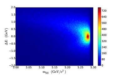
(a) $B^{-}\rightarrow\mathchar 28931\relax_{c}^{+}\overline{p}e^{-}\overline{\nu}_{e}$ Signal Monte Carlo

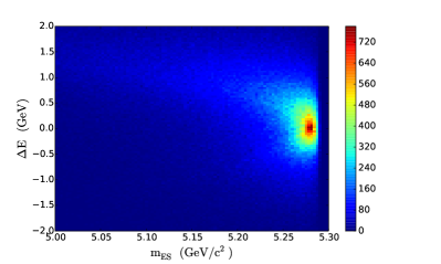
(b) $B^{-}\rightarrow\mathchar 28931\relax_{c}^{+}\overline{p}\mu^{-}\overline{\nu}_{\mu}$ Signal Monte Carlo

Figure 5.3: The $\Delta E$-$m_{\rm ES}$ plane in WI signal Monte Carlo for the two $B^{-}\rightarrow\mathchar 28931\relax_{c}^{+}\overline{p}\ell^{-}\nu_{\ell}$ signal modes.

Furthermore, the distributions show that the signal has large tails in $m_{\rm ES}$ as well as in $\Delta E$.

Chapter 6 Background suppression

For a good separation of signal and background a detailed background study is necessary. Therefore, we identified two different classes of background.

1. continuum events from $e^{+}e^{-}\rightarrow q\overline{q}$ ($q=u,d,s,c$)

2. combinatorial background from other $B$ decays

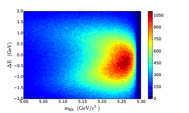
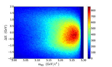
Figure 6.1: The $\Delta E$-$m_{\rm ES}$ plane for $uds$ 6.1 and $c\overline{c}$ 6.1 Monte Carlo.

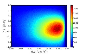
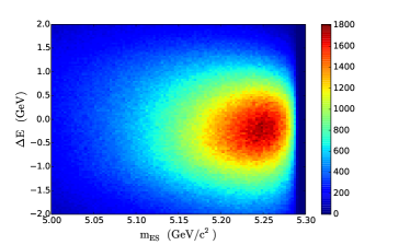
Figure 6.2: The $\Delta E$-$m_{\rm ES}$ plane for $B^{+}{\kern-1.60004ptB^{-}}$ 6.2 and $B^{0}{\kern-1.60004pt\kern 1.79993pt\overline{\kern-1.79993ptB}{}^{0}}$ 6.2 Monte Carlo.

The two-dimensional $\Delta E$-$m_{\rm ES}$ distribution for these two background classes after the decay reconstruction can be found in Figures 6.1 and 6.2. In comparison to the signal Monte Carlo distribution shown in Figure 5.3 these two background classes are smeared out over a large phase space region. In addition, the $uds$ background shown in Fig. 6.1 is shifted to smaller $m_{\rm ES}$ values. Note, that the concentration of background events close the the signal region is caused by the large invariant mass of the $Y$ system.

6.1 $\mathchar 28931\relax_{c}^{+}$ mass cut

In order to suppress background from generic $p$, $K^{-}$ and $\pi^{+}$ combinations in the $\mathchar 28931\relax_{c}^{+}$ reconstruction we decide to use a $\pm 3\sigma$ mass selection region around the central mass value of the $\mathchar 28931\relax_{c}^{+}$. Due to the observed difference between OnPeak data and Monte Carlo events the cut has to be determined separately for both data sets. Therefore, we fit the $m(\mathchar 28931\relax_{c}^{+})$ distribution in data and signal Monte Carlo with a Gaussian $g(m;\mu,\sigma)$ for signal and a second order Chebychev polynomial $p(m;b_{1},b_{2})$ for background. The fit results are given in Fig. 6.3, 6.4 and Table 6.1, and 6.2. Due to the high statistics of the signal Monte Carlo sample a better fit would require additional terms for signal description. But for the purpose of a mass cut the shown description suffices.

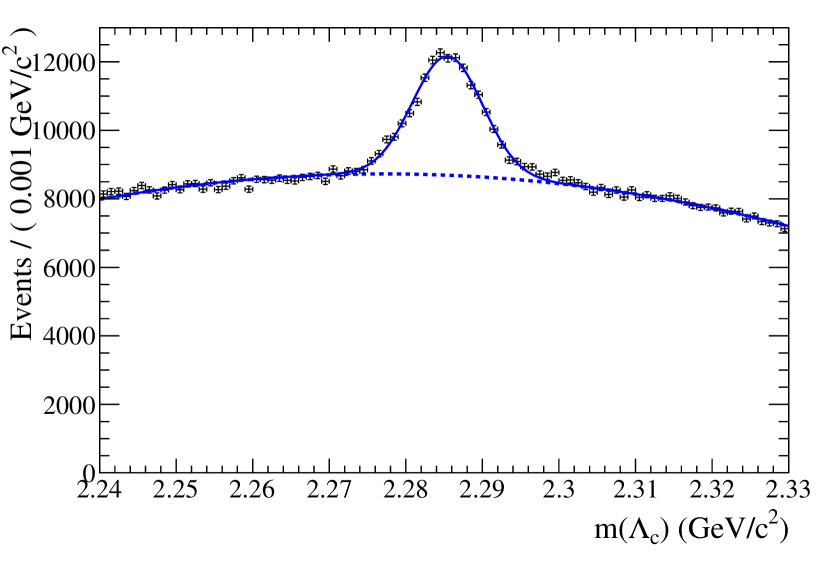
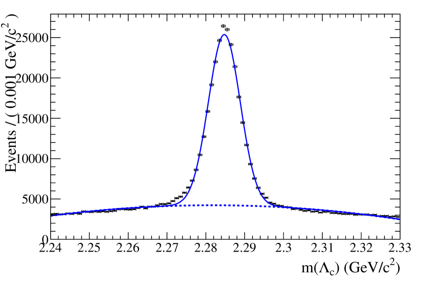
Figure 6.3: $m(\mathchar 28931\relax_{c}^{+})$ fit in OnPeak data.	Figure 6.4: $m(\mathchar 28931\relax_{c}^{+})$ fit in $B^{-}\rightarrow\mathchar 28931\relax_{c}^{+}\overline{p}e^{-}\overline{\nu}_{e}$ MC events.
Table 6.1: Fit parameter for a fit to $m(\mathchar 28931\relax_{c}^{+})$ in data events. parameter value $N_{bkg}$ $749530\pm 1120$ $N_{sig}$ $39835\pm 739$ $\mu$ $2.285453\pm 0.000068$ $\sigma$ $0.004578\pm 0.000081$ $b_{1}$ $-0.04754\pm 0.0020$ $b_{2}$ $-0.06730\pm 0.0026$	Table 6.2: Fit parameter for a fit to $m(\mathchar 28931\relax_{c}^{+})$ in Monte Carlo events. parameter value $N_{bkg}$ $334006\pm 744$ $N_{sig}$ $217413\pm 661$ $\mu$ $2.284760\pm 0.000012$ $\sigma$ $0.004099\pm 0.000013$ $b_{1}$ $-0.06399\pm 0.0030$ $b_{2}$ $-0.21995\pm 0.0038$

The fit returns a $\sigma$ of $4.58\pm 0.09{\mathrm{\,Me\kern-1.00006ptV\!/}c^{2}}$ for data and $4.10\pm 0.02{\mathrm{\,Me\kern-1.00006ptV\!/}c^{2}}$ for Monte Carlo. The larger value for data events is plausible taking into account the observed momentum dependence of the mean value of the $\mathchar 28931\relax_{c}^{+}$ mass for data [42]. Since we use $\mathchar 28931\relax_{c}^{+}$ candidates from a relatively large momentum range this effect leads to a broader distribution.

For convenience we decide to use the same width for the cut for both, OnPeak data and Monte Carlo, only shifted according to the different mean values, measured in section 5.1.1. Therefore, we decide to use the following cut on the $\mathchar 28931\relax_{c}^{+}$ candidate mass for data

$$2.2716<m(\mathchar 28931\relax_{c}^{+})<2.2992{\mathrm{\,Ge\kern-1.00006ptV\!/}c^{2}},$$ (6.1)

corresponding to $\pm 3\sigma$, and for Monte Carlo

$$2.2711<m(\mathchar 28931\relax_{c}^{+})<2.2987{\mathrm{\,Ge\kern-1.00006ptV\!/}c^{2}},$$ (6.2)

corresponding to $\pm 3.4\sigma$.

6.2 Particle identification

For the reconstruction of our signal candidates we use the PID lists used in the BABAR internal data reprocessing. While the CombinedSuperLoose PID lists provide a high probability to correctly identify the detected tracks they have a high mis-identification probability as well. In order to reduce the number of mis-identified particles we decide to use the more stringent PID lists, given in Table 6.3.

Table 6.3: Particle ID lists used for the signal extraction.

particle	PID list
proton ($\mathchar 28931\relax_{c}^{+}$)	pKMLoose
kaon ($\mathchar 28931\relax_{c}^{+}$)	KKMLoose
pion ($\mathchar 28931\relax_{c}^{+}$)	piKMLoose
proton	pKMTight
electron	eKMTight
muon	muBDTTight

6.3 Continuum background suppression

For the reduction of continuum background ($q\overline{q}$, $q=u,d,s,c$) we decide to use a random forest. The number of split variables is set to $\sqrt{p}$, where $p$ is the total number of discriminating variables. The training data sets for signal and background equal each other in size.

For continuum background we settle on three event shape variables, defined as:

• The ratio of the second and zeroth Fox-Wolfram moment $R_{2}$ [43] for all charged tracks, defined as

  $$R_{2}=\frac{\sum_{ij}^{tracks}|p_{i}||p_{j}|P_{2}(\cos\theta_{ij})}{\sum_{ij}^{tracks}|p_{i}||p_{j}|},$$ (6.3)

  with the Legendre polynomial $P_{2}$ and the angle $\theta_{ij}$ between the momenta $p_{i}$ and $p_{j}$.

• The sphericity $S$ of the event [43], derived from the sphericity tensor

  $$S^{\alpha\beta}=\frac{\sum_{i}p_{i}^{\alpha}p_{i}^{\beta}}{\sum_{i}|\vec{p}_{i}|^{2}},$$ (6.4)

  where $\alpha,\beta=1,2,3$ correspond to the $x$, $y$ and $z$ components.

• The cosine of the angle between the thrust axis of the $Y$ candidate and the thrust axis [43] of the rest of the event $\cos\Delta\theta_{\rm thrust}$. The thrust axis is defined as the unit vector $\vec{n}$ that maximizes the thrust $T$

  $$T=\max_{|\vec{n}|=1}\frac{\sum_{i}^{tracks}|\vec{n}\cdot\vec{p}_{i}|}{\sum_{i}|\vec{p}_{i}|}.$$ (6.5)

A comparison of these three variables between signal and background for the electron channel is given in Fig. 6.5, and for the muon channel in the appendix, Fig. A.1.

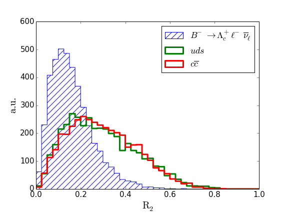
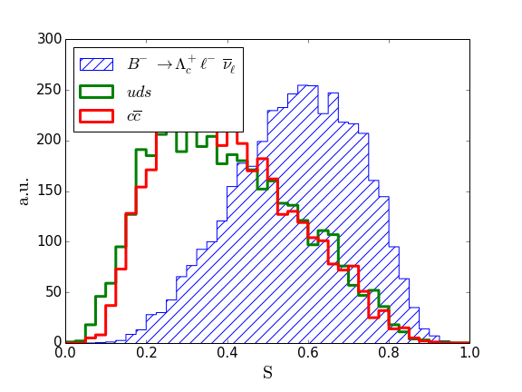
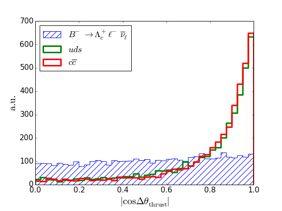
Figure 6.5: Comparison of WI signal Monte Carlo (blue histogram) and $q\overline{q}$ background Monte Carlo (green and red lines) for the three Random Forest input variables, 6.5 $R_{2}$, 6.5 $S$, and 6.5 $cos\Delta\theta_{\rm thrust}$.

The random forest (RF) has two major variables to be adjusted for optimal performance, the number of trees $N_{\rm trees}$ and the minimum number of events per leaf $N_{\rm leaf}$. We optimise these two variables by training random forests with both variables ranging from $10$ to $1000$ and calculating the area $A$ below the receiver operating characteristic (ROC) curve. A large value here points to a good performance. A plot of the area in dependence of $N_{\rm trees}$ and $N_{\rm leaf}$ can be seen in Fig. 6.6. The optimum for the RF configuration is at $380$ trees and $60$ events per leaf, but as can be seen from Fig. 6.6 the variation in $A$ is not very large (except close to $N_{\rm trees}=0$), and in consequence the performance deficits by using a not optimal configuration are negligible.

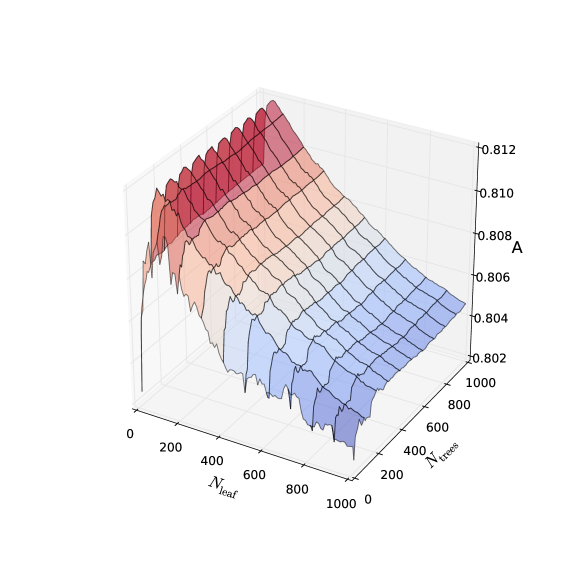
Figure 6.6: Area below the ROC curve in dependence of $N_{\rm trees}$ and $N_{\rm leaf}$.

For continuum background we decide to use the optimal set of $N_{\rm trees}=380$ and $N_{\rm leaf}=60$ for the electron and the muon channel. The classifier distribution for signal and background after training is shown in Fig. 6.7.

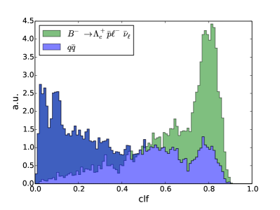
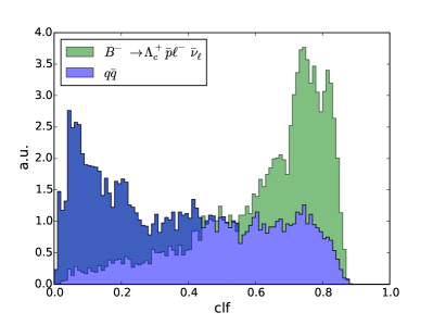
Figure 6.7: The classifier distributions for signal and background after training of the random forest: 6.7 $B^{-}\rightarrow\mathchar 28931\relax_{c}^{+}\overline{p}e^{-}\overline{\nu}_{e}$, 6.7 $B^{-}\rightarrow\mathchar 28931\relax_{c}^{+}\overline{p}\mu^{-}\overline{\nu}_{\mu}$.

Maximizing $S/\sqrt{S+B}$, with the signal yield $S$ scaled to an expected branching fraction of $10^{-4}$ and the background yield $B$ (including $B{\kern-1.60004pt\kern 1.79993pt\overline{\kern-1.79993ptB}{}}$ background) scaled to data luminosity, returns an optimal cut of $>0.4$ for the electron case, preserving $88\%$ of the signal, while reducing continuum background to $41\%$. For the muon channel we obtain an optimal cut of $>0.4$ as well, preserving $87\%$ of the signal and reducing background to $42\%$. A comparison of signal and background efficiency in dependence of the classifier cut is shown in Fig. 6.8.

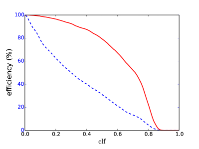
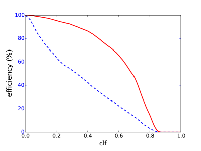
Figure 6.8: Signal (red, solid line) and background (blue, dashed line) efficiencies in dependence of the cut on the random forest classifier: 6.7 $B^{-}\rightarrow\mathchar 28931\relax_{c}^{+}\overline{p}e^{-}\overline{\nu}_{e}$, 6.7 $B^{-}\rightarrow\mathchar 28931\relax_{c}^{+}\overline{p}\mu^{-}\overline{\nu}_{\mu}$.

6.4 $B$ background suppression

In the next step after continuum background reduction we have to reduce generic $B{\kern-1.60004pt\kern 1.79993pt\overline{\kern-1.79993ptB}{}}$ background as well. Therefore, we train an additional random forest, based on four input variables:

• The lepton momentum in the CM system,

• the angle between the lepton momentum and the momentum of the $\mathchar 28931\relax_{c}^{+}\overline{p}$ system in the CM frame,

• the vertex probability for the $Y$ candidate, and

• the transverse neutrino momentum in the CM system.

A comparison of WI signal Monte Carlo and generic $B$ Monte Carlo data is shown in Fig. 6.9 for the electron and in the appendix (Fig. A.2) for muons. For the vertex probability signal as well as background contain events with a vertex probability of zero. But, the fraction of these candidates in the background is much larger. As shown in the inset the number of events with a probability larger $0.1$ stays nearly constant for the signal simulation, while it converges to zero for background events.

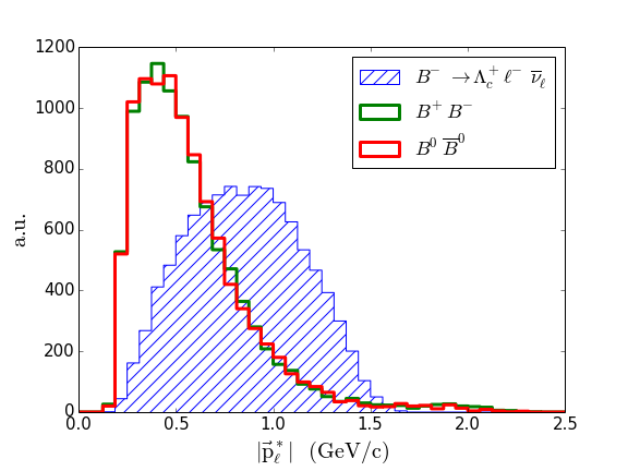
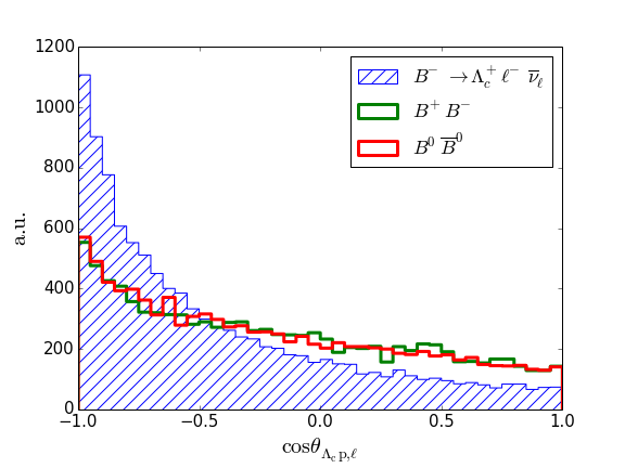
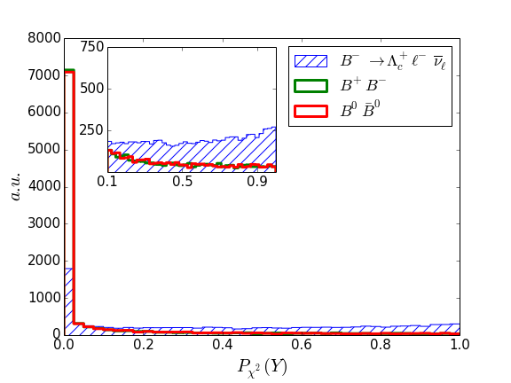
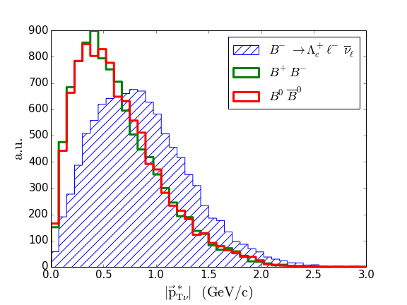
Figure 6.9: Comparison of WI signal simulation events and generic $B$ decays: 6.9 $|\vec{p}_{\ell}^{*}|$, 6.9 $\cos\theta_{\mathchar 28931\relax_{c}p,\ell}$, 6.9 $P_{\chi^{2}}(Y)$, and 6.9 $p_{T\nu}$.

As for the $q\overline{q}$ background we optimize the $B{\kern-1.60004pt\kern 1.79993pt\overline{\kern-1.79993ptB}{}}$ random forest as well. For performance reasons we decide to vary the number of trees between $100$ and $500$ and the number of events per leaf between $10$ and $200$. The resulting distribution of the area below the ROC curve can be seen in Fig. 6.10. The optimal RF performance is achieved with $450$ trees and a minimum number of $40$ events per leaf. As for the $q\overline{q}$ RF the variation of the area below the ROC curve is rather small, for $N_{\rm trees}>>100$. The classifier distributions for signal and background are shown in Fig. 6.11.

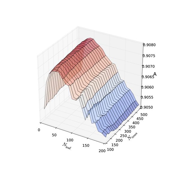
Figure 6.10: Area below the ROC curve in dependence of $N_{\rm trees}$ and $N_{\rm leaf}$.

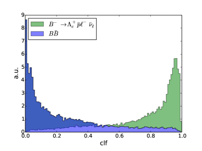
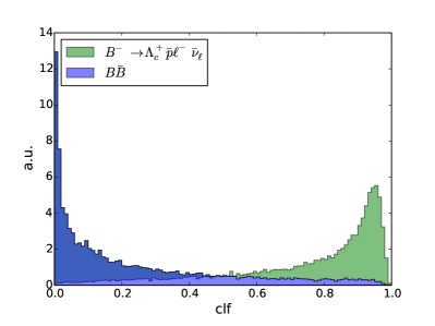
Figure 6.11: The classifier distributions for signal and background after training of the $B{\kern-1.60004pt\kern 1.79993pt\overline{\kern-1.79993ptB}{}}$ random forest: 6.11 $B^{-}\rightarrow\mathchar 28931\relax_{c}^{+}\overline{p}e^{-}\overline{\nu}_{e}$, 6.11 $B^{-}\rightarrow\mathchar 28931\relax_{c}^{+}\overline{p}\mu^{-}\overline{\nu}_{\mu}$.

6.4.1 $B{\kern-1.60004pt\kern 1.79993pt\overline{\kern-1.79993ptB}{}}$ Classifier as fit variable

A possible fit variable is the Random Forest output for the $B{\kern-1.60004pt\kern 1.79993pt\overline{\kern-1.79993ptB}{}}$ background itself. This variable offers by construction a good separation of signal and background, as can be seen in Fig. 6.12. In addition the agreement between the background Monte Carlo and the data distribution within the uncertainties is reasonable for low values, although it seems to underestimate background a little. For large values the background Monte Carlo simulation overestimates data background.

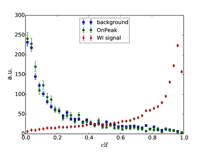
Figure 6.12: Comparison of background Monte Carlo (blue squares), OnPeak data (green dots) and WI signal Monte Carlo (red diamonds) for the $B{\kern-1.60004pt\kern 1.79993pt\overline{\kern-1.79993ptB}{}}$ Random Forest classifier.

Another problem arises when it comes to find a functional description of the signal distribution. A closer look at large classifier ($clf$) values, as shown in Fig. 6.13 for the electron channel, shows a shoulder on the right hand side of the signal peak, as well as some structure on the left side. This would require a rather complex fit function, which strongly depends on the specific decay model. Thus, we decide not to use the classifier as a fit variable, but rather select candidates above a certain threshold in the classifier.

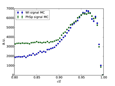
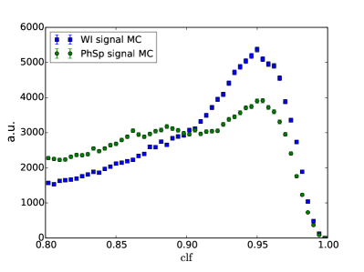
Figure 6.13: The $B{\kern-1.60004pt\kern 1.79993pt\overline{\kern-1.79993ptB}{}}$ classifier distribution for the WI electron 6.13 and muon 6.13 signal Monte Carlo. The blue squares show the WI model, and the green dots the phase space model. Shown is the range from $0.8$ to $1.0$.

Chapter 7 Analysis

For the further analysis of the decay we select events above a certain threshold in the $B{\kern-1.60004pt\kern 1.79993pt\overline{\kern-1.79993ptB}{}}$ classifier. The optimal value of this threshold is determined by maximizing the statistical significance $S/\sqrt{S+B}$, where $S$ is the expected signal yield, and $B$ the background yield. Here, we use all events that passed the previously described selection criteria. For the background yield we scale the $q\overline{q}$ and $B{\kern-1.60004pt\kern 1.79993pt\overline{\kern-1.79993ptB}{}}$ Monte Carlo data sets to OnPeak luminosity. For the signal yield we vary the expected branching fraction between $0.5\times 10^{-5}$ and $5\times 10^{-4}$. Fig. 7.1 shows $S/\sqrt{S+B}$ versus the classifier cut for both signal channels. The maximal value for the electron channel is achieved for $clf>0.9$, reducing background to $2\%$ while preserving $36\%$ of signal. The maximum for the muon channel is at $>0.85$, reducing background to $3\%$ while preserving $42\%$ of signal. Both optimal cuts show no significant variation with the expected signal yield.

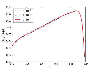
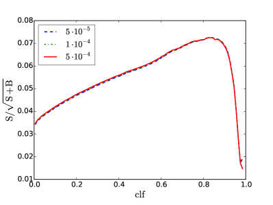
Figure 7.1: $S/\sqrt{S+B}$ versus the $B{\kern-1.60004pt\kern 1.79993pt\overline{\kern-1.79993ptB}{}}$ classifier for the electron 7.1 and muon 7.1 channel.

Figure 7.2 shows a comparison of background and signal efficiency in dependence of the classifier cut for both signal channels.

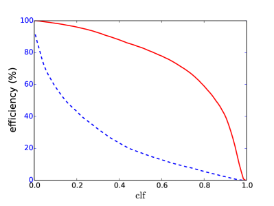
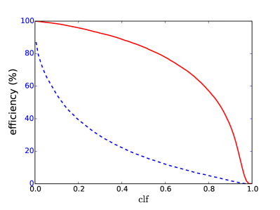
Figure 7.2: Signal (red, solid line) and background (blue, dashed line) efficiencies in dependence of the cut on the random forest classifier. 6.11 $B^{-}\rightarrow\mathchar 28931\relax_{c}^{+}\overline{p}e^{-}\overline{\nu}_{e}$, 6.11 $B^{-}\rightarrow\mathchar 28931\relax_{c}^{+}\overline{p}\mu^{-}\overline{\nu}_{\mu}$.

7.1 Fit variable

For signal extraction we have two possible sets of variables to determine the signal yield, first the classic neutrino variables

• $m^{2}_{\rm miss}=E^{2}_{\rm miss}-\vec{p}^{2}_{\rm miss}$

• $m^{2}_{\rm miss}/2E_{\rm miss}$

• $m_{\nu}^{2}=(E_{\rm beam}^{*}-E_{Y}^{*})^{2}-\vec{p}^{*2}_{Y}$

where $E_{\rm beam}$, $E_{Y}^{*}$ and $\vec{p}_{Y}^{*}$ are measured in the CM system. For $m_{\nu}^{2}$ we neglect the small momentum of the $B$ meson in the CM system, in consequence the neutrino momentum and the momentum of the Y system have the same magnitude. The second set consists of

• $\Delta E$

• $m_{\rm ES}$,

as defined in eq. (5.5) and (5.6).

Crucial for both variable sets is a good description of the background shape by background Monte Carlo, and different shapes for background and signal. The next sections show a comparison of background Monte Carlo with OnPeak data and with WI signal Monte Carlo to decide on the variables for signal extraction. If the background description from generic Monte Carlo is capable of describing data background we expect a good agreement between background Monte Carlo events and OnPeak data, with a possible variation due to a signal component in data.

7.1.1 Neutrino Variables

All three neutrino variables work well for low-mass final states like $B\rightarrow\pi\ell\nu$, but might have problems with high-mass final states, as it can be seen in the analysis of $B^{-}\rightarrow D_{s}^{+}K^{-}\ell^{-}\overline{\nu}_{\ell}$ [44]. In this analysis the signal yield was extracted in $m^{2}_{\rm miss}$, but in contrast to decays like $B\rightarrow\pi\ell\nu$ background in this variable is not flat. In consequence, the signal peak had to be fitted onto a steep slope. The situation might be even more difficult in the present analysis, where the final state is about $0.8{\mathrm{\,Ge\kern-1.00006ptV\!/}c^{2}}$ heavier.

A comparison between background Monte Carlo events, OnPeak data, and WI signal Monte Carlo data for these three variables is shown in Fig. 7.3. The comparison of background and signal Monte Carlo events for $m^{2}_{\rm miss}$ and $m^{2}_{\rm miss}/2E_{\rm miss}$ shows that the distributions equal each other. This can be explained in terms of the large invariant mass of the $Y$ system, leaving only a small fraction of energy and momentum for the neutrino, in consequence a neutrino signature can be easily faked by a wrong particle identification in the neutrino reconstruction, or a missing photon.

In contrast $m_{\nu}^{2}$ is independent of the particle identification in the neutrino reconstruction and offers a small difference between background and signal. In addition the agreement between the OnPeak and the background Monte Carlo distribution is reasonably good, making $m_{\nu}^{2}$ a possible fit variable. The down-side of $m_{\nu}^{2}$ as fit variable is that a fit in this quantity requires to fit the signal on the right slope of the background distribution.

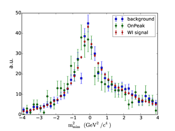
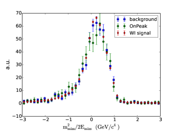
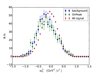
Figure 7.3: Comparison of background Monte Carlo (blue squares), OnPeak data (green dots) and WI signal Monte Carlo (red diamonds) for the three neutrino variables 7.3 $m^{2}_{\rm miss}$, 7.3 $m^{2}_{\rm miss}/2E_{\rm miss}$, and 7.3 $m_{\nu}^{2}$.

7.1.2 $B$ Variables

Two other possible target variables are $m_{\rm ES}$ and $\Delta E$ for the reconstructed $B$ meson. Fig. 7.4 shows a comparison between data and Monte Carlo for these two variables. Comparing the $m_{\rm ES}$ distributions we see a good separation between background and signal, as well as a reasonable agreement between the background Monte Carlo and data distributions. This makes $m_{\rm ES}$ a good choice as fit variable. In contrast the $\Delta E$ distribution shows a rather similar shape for background and signal Monte Carlo events.

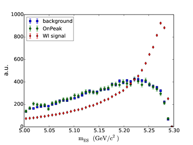
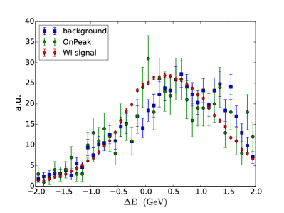
Figure 7.4: Comparison of background Monte Carlo (blue squares), OnPeak data (green dots) and WI signal Monte Carlo (red diamonds) for 7.4 $m_{\rm ES}$, and 7.4 $\Delta E$.

7.2 Signal extraction

For signal extraction we decide to perform a simultaneous maximum likelihood fit in $m_{\rm ES}$ and $m_{\nu}^{2}$. Therefore, it is crucial to exclude a strong correlation between these two variables. Fig. 7.5 shows no correlation between these two variables, neither for signal nor for background. To exclude the possibility that the shape in one variable varies in dependence of the second variable, we compare the projections in slices of the second variable as well. Fig. C.1 and C.2 show these projections for WI signal and background Monte Carlo. There seems to be no strong variation in shape parameters for neither signal, nor background. Thus, we can apply a factorization ansatz. In the following sections we determine the parameters of the background and signal probability density functions (pdf) by fitting Monte Carlo events.

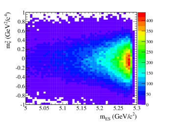
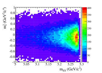
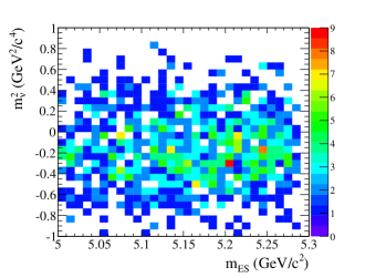
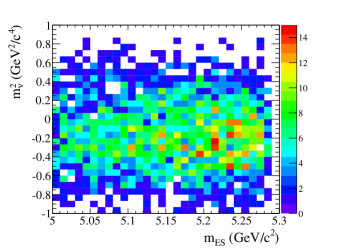
Figure 7.5: $m_{\nu}^{2}:\mbox{$m_{\rm ES}$}$ plane for WI signal Monte Carlo 7.5,7.5 and generic background Monte Carlo data 7.5, 7.5. For the electron channel 7.5, 7.5, and for the muon channel 7.5, 7.5.

7.2.1 Signal parametrization

For signal description we decide to use for $m_{\nu}^{2}$ a Cruijff function $C(x;m_{0},\sigma_{L},\sigma_{R},\alpha_{L},\alpha_{R})$ defined as

$$C(x;m_{0},\sigma_{L},\sigma_{R},\alpha_{L},\alpha_{R})=\begin{cases}\exp{\left(\frac{-(x-m_{0})^{2}}{2\cdot\sigma_{R}^{2}+\alpha_{R}\cdot(x-m_{0})^{2}}\right)}&\text{if }x-m_{0}>0\\ \\ \exp{\left(\frac{-(x-m_{0})^{2}}{2\cdot\sigma_{L}^{2}+\alpha_{L}\cdot(x-m_{0})^{2}}\right)}&\text{if }x-m_{0}\leq 0,\end{cases}$$ (7.1)

and the sum of an ARGUS function ${\cal A}(x;c,p,m_{0})$ and a Novosibirsk function ${\cal N}(x;x_{0},\sigma,\mathchar 28931\relax)$ for $m_{\rm ES}$.

$$S(x;c,p,m_{0},x_{0},\sigma,\mathchar 28931\relax,f_{1}) =f_{1}\cdot{\cal A}(x;c,p,)+(1-f_{1})\cdot{\cal N}(x;x_{0},\sigma,\mathchar 28931\relax)$$ (7.2)

The ARGUS function ${\cal A}(x;c,p,m_{0})$ is defined as

$${\cal A}(x;c,p) =x\cdot\left(1-\left(\frac{x}{m_{0}}\right)^{2}\right)^{p}\cdot\exp{\left(c\cdot\left(1-\left(\frac{x}{m_{0}}\right)^{2}\right)\right)},$$ (7.3)

where $m_{0}$ denotes the upper boundary which coincides with half the center of mass energy in BABAR, and can thus be taken from data as a conditional observable. The parameters $p$ and $c$ determine the shape of the ARGUS function. In the definition [45] first used by the ARGUS collaboration $p$ is fixed to $0.5$. To reduce the number of free parameters we will do the same here.
The Novosibirsk distribution ${\cal N}(x;x_{0},\sigma,\mathchar 28931\relax)$ is defined as

$${\cal N}(x;x_{0},\sigma,\mathchar 28931\relax) =\exp{\left(-\frac{1}{2}\frac{(\ln q_{y})^{2}}{\mathchar 28931\relax^{2}}+\mathchar 28931\relax^{2}\right)}$$ (7.4)

$$q_{y} =1+\frac{\mathchar 28931\relax(x-x_{0})}{\sigma}\cdot\frac{\sinh\left(\mathchar 28931\relax\sqrt{\ln 4}\right)}{\mathchar 28931\relax\sqrt{\ln 4}},$$ (7.5)

where $x_{0}$ represents the peak position, $\sigma$ the width of the peak, and $\mathchar 28931\relax$ the asymmetric tail. For the fit only correctly reconstructed events are considered. Thus, we can determine the signal parameters, without a pollution from background events.

The fitted $m_{\nu}^{2}$ distributions are shown in Fig. 7.6 and the fit parameters in Table 7.1. For the $m_{\rm ES}$ fit the fitted signal distributions are shown in Fig. 7.7, and the fit parameters in Tab. 7.2.

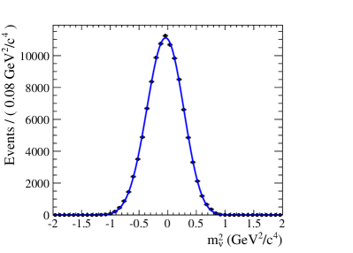
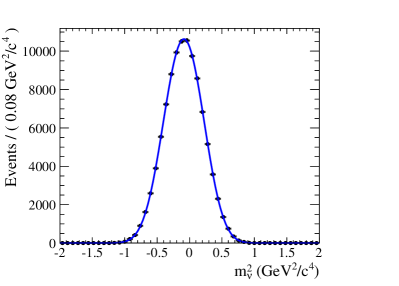
Figure 7.6: Fitted $m_{\nu}^{2}$ distribution for WI signal Monte Carlo data: 7.6 for $B^{-}\rightarrow\mathchar 28931\relax_{c}^{+}\overline{p}e^{-}\overline{\nu}_{e}$, and 7.6 for $B^{-}\rightarrow\mathchar 28931\relax_{c}^{+}\overline{p}\mu^{-}\overline{\nu}_{\mu}$.

Table 7.1: Parameters for the fit to the $m_{\nu}^{2}$ distribution for WI signal Monte Carlo events: 7.1 for $B^{-}\rightarrow\mathchar 28931\relax_{c}^{+}\overline{p}e^{-}\overline{\nu}_{e}$, and 7.1 for $B^{-}\rightarrow\mathchar 28931\relax_{c}^{+}\overline{p}\mu^{-}\overline{\nu}_{\mu}$.

parameter	value
$m_{0}$	$-0.035$ $\pm$	$0.005$
$\sigma_{L}$	$0.326$ $\pm$	$0.004$
$\sigma_{R}$	$0.316$ $\pm$	$0.004$
$\alpha_{L}$	$-0.023$ $\pm$	$0.005$
$\alpha_{R}$	$-0.044$ $\pm$	$0.006$

parameter	value
$m_{0}$	$-0.086$ $\pm$	$0.004$
$\sigma_{L}$	$0.314$ $\pm$	$0.004$
$\sigma_{R}$	$0.310$ $\pm$	$0.004$
$\alpha_{L}$	$-0.035$ $\pm$	$0.006$
$\alpha_{R}$	$-0.039$ $\pm$	$0.006$

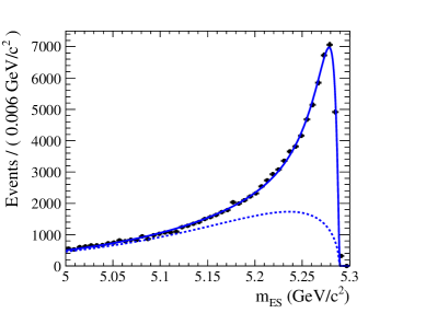
Figure 7.7: Fitted $m_{ES}$ distribution for WI signal Monte Carlo data: 7.7 for $B^{-}\rightarrow\mathchar 28931\relax_{c}^{+}\overline{p}e^{-}\overline{\nu}_{e}$, and 7.7 for $B^{-}\rightarrow\mathchar 28931\relax_{c}^{+}\overline{p}\mu^{-}\overline{\nu}_{\mu}$.

Table 7.2: Parameters for the fit to the $m_{ES}$ distribution for WI signal Monte Carlo events. 7.2 for $B^{-}\rightarrow\mathchar 28931\relax_{c}^{+}\overline{p}e^{-}\overline{\nu}_{e}$, and 7.2 for $B^{-}\rightarrow\mathchar 28931\relax_{c}^{+}\overline{p}\mu^{-}\overline{\nu}_{\mu}$.

parameter	value
$c$	$-24.9$ $\pm$	$0.6$
$f_{1}$	$0.514$ $\pm$	$0.020$
$x_{0}$	$5.27930$ $\pm$	$0.00015$
$\sigma$	$0.0144$ $\pm$	$0.0004$
$\mathchar 28931\relax$	$1.32$ $\pm$	$0.05$

parameter	value
$c$	$-24.5$ $\pm$	$0.6$
$f_{1}$	$0.542$ $\pm$	$0.021$
$x_{0}$	$5.27950$ $\pm$	$0.00016$
$\sigma$	$0.0142$ $\pm$	$0.0005$
$\mathchar 28931\relax$	$1.34$ $\pm$	$0.05$

In order to assess the quality of the fit we can check the binned two-dimensional pull $p$

$$p_{i}=\frac{f_{i}(m_{\nu}^{2},\mbox{$m_{\rm ES}$})-N_{i}(m_{\nu}^{2},\mbox{$m_{\rm ES}$})}{\sigma_{i}},$$ (7.6)

where $N_{i}(m_{\nu}^{2},\mbox{$m_{\rm ES}$})$ is the number of entries in the $i$-th bin, and $\sigma$ the uncertainty on $N_{i}$. The pull distributions are shown in Fig. 7.8. The pull plots show a systematic deviation at large $m_{\rm ES}$ values and $m_{\nu}^{2}\approx 0.4\mathrm{\,Ge\kern-1.00006ptV}^{2}/c^{4}$. This deviation is not accounted for in the simultaneous fit, since an unbinned two-dimensional fit without correlations equals a simultaneous fit in the $m_{\nu}^{2}$ and $m_{\rm ES}$ distribution. As for a simultaneous fit only the agreement in the projections is relevant, which is good. The pull plots are only shown for completeness.

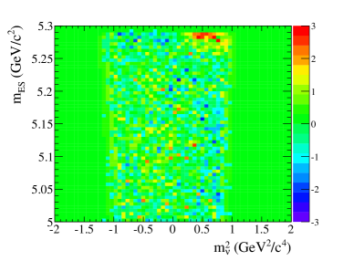
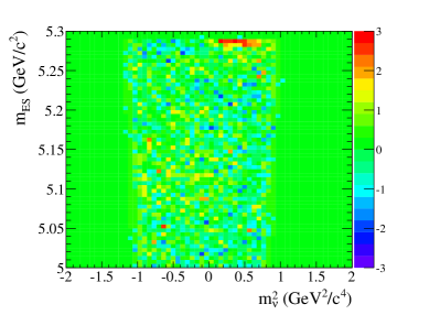
Figure 7.8: Pull plots for the fit to WI signal Monte Carlo data: 7.8 for $B^{-}\rightarrow\mathchar 28931\relax_{c}^{+}\overline{p}e^{-}\overline{\nu}_{e}$, and 7.8 for $B^{-}\rightarrow\mathchar 28931\relax_{c}^{+}\overline{p}\mu^{-}\overline{\nu}_{\mu}$.

7.2.2 Background parametrization

For background we use a Cruijff function for $m_{\nu}^{2}$ as well, and for $m_{\rm ES}$ an ARGUS function. For the ARGUS we leave the exponent $p$ floating to allow for a steeper distribution. The fitted projections are shown in Fig. 7.9 and 7.10, and the parameters are given in Tab. 7.3 and 7.4. The input data set for the fit consists of a luminosity scaled mixture of $q\overline{q}$ and $B{\kern-1.60004pt\kern 1.79993pt\overline{\kern-1.79993ptB}{}}$ Monte Carlo events, i.e. the relative contributions of $q\overline{q}$ and $B{\kern-1.60004pt\kern 1.79993pt\overline{\kern-1.79993ptB}{}}$ events to the complete input set are equivalent to the expected ratios in OnPeak data. The corresponding pull plots, shown in Fig. 7.11, show no systematic deviations between the fitted function and the background Monte Carlo data.

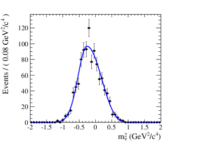
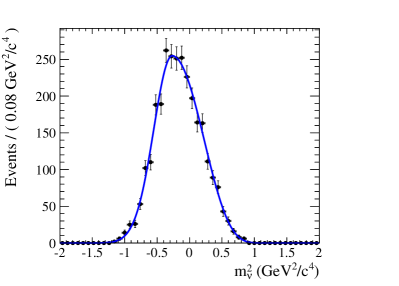
Figure 7.9: Fitted $m_{\nu}^{2}$ distribution for background Monte Carlo data: 7.9 for $B^{-}\rightarrow\mathchar 28931\relax_{c}^{+}\overline{p}e^{-}\overline{\nu}_{e}$, and 7.9 for $B^{-}\rightarrow\mathchar 28931\relax_{c}^{+}\overline{p}\mu^{-}\overline{\nu}_{\mu}$.

Table 7.3: Fit parameters for the fit to the $m_{\nu}^{2}$ distribution for background Monte Carlo events: 7.3 for $B^{-}\rightarrow\mathchar 28931\relax_{c}^{+}\overline{p}e^{-}\overline{\nu}_{e}$, and 7.3 for $B^{-}\rightarrow\mathchar 28931\relax_{c}^{+}\overline{p}\mu^{-}\overline{\nu}_{\mu}$.

parameter	value
$m_{0}$	$-0.26$ $\pm$	$0.04$
$\sigma_{L}$	$0.271$ $\pm$	$0.030$
$\sigma_{R}$	$0.44$ $\pm$	$0.04$
$\alpha_{L}$	$0.01$ $\pm$	$0.04$
$\alpha_{R}$	$-0.10$ $\pm$	$0.08$

parameter	value
$m_{0}$	$-0.268$ $\pm$	$0.025$
$\sigma_{L}$	$0.283$ $\pm$	$0.022$
$\sigma_{R}$	$0.469$ $\pm$	$0.029$
$\alpha_{L}$	$0.007$ $\pm$	$0.028$
$\alpha_{R}$	$-0.13$ $\pm$	$0.04$

Table 7.4: Fit parameters for the fit to the $m_{ES}$ distribution for background Monte Carlo events: 7.4 for $B^{-}\rightarrow\mathchar 28931\relax_{c}^{+}\overline{p}e^{-}\overline{\nu}_{e}$, and 7.4 for $B^{-}\rightarrow\mathchar 28931\relax_{c}^{+}\overline{p}\mu^{-}\overline{\nu}_{\mu}$.

parameter	value
$c$	$-16.5$ $\pm$	$1.1$
$p$	$0.45$ $\pm$	$0.08$

parameter	value
$c$	$-15.7$ $\pm$	$0.07$
$p$	$0.3976$ $\pm$	$0.0010$

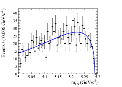
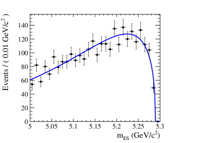
Figure 7.10: Fitted $m_{ES}$ distribution for background Monte Carlo data. 7.10 for $B^{-}\rightarrow\mathchar 28931\relax_{c}^{+}\overline{p}e^{-}\overline{\nu}_{e}$, and 7.10 for $B^{-}\rightarrow\mathchar 28931\relax_{c}^{+}\overline{p}\mu^{-}\overline{\nu}_{\mu}$.

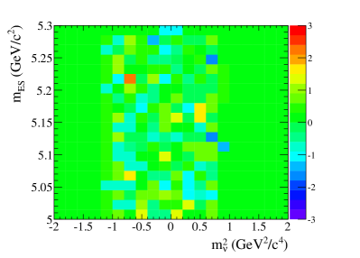
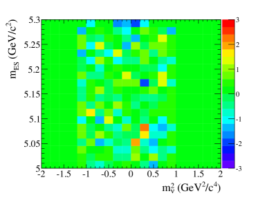
Figure 7.11: Pull plots for the fit to background Monte Carlo data: 7.11 for $B^{-}\rightarrow\mathchar 28931\relax_{c}^{+}\overline{p}e^{-}\overline{\nu}_{e}$, and 7.11 for $B^{-}\rightarrow\mathchar 28931\relax_{c}^{+}\overline{p}\mu^{-}\overline{\nu}_{\mu}$.

7.2.3 Fit validation

In order to validate the fit procedure, and exclude any significant systematic uncertainties in the extracted signal yield, we prepare different mixtures of background and signal Monte Carlo data. While the used background set stays the same we vary the signal fraction from $\mathrm{𝟎}$ to $100$ events and compare the fitted signal yields with the size of the input data sets. Table 7.5, listing the fit result, shows no significant deviations between the size of the input data set and the fitted signal yield. Thus, we conclude that the fit procedure does not lead to a significant over- or underestimation of the signal yield and is save to use for signal extraction. The fits are shown in Fig. C.3 and C.4.

Table 7.5: Size of the signal input data set, and the fitted signal yield for the electron and muon channel.

signal events	$e^{-}$ fit result	$\mu^{-}$ fit result
$100$	$80\pm 40$	$100\pm 70$
$50$	$30\pm 40$	$60\pm 70$
$10$	$10\pm 40$	$20\pm 70$
$\mathrm{𝟎}$	$-1\pm 40$	$30\pm 70$

7.2.4 Fit to data

We extract the signal yield for both signal channels on data separately. Therefore, all parameters of the background and signal pdfs are fixed to their optimal values, determined in section 7.2.1 and 7.2.2. The fitted distributions and the pull distribution are shown in Fig. 7.12, 7.13, and 7.14. The obtained signal yields are

$$N_{\rm sig}(B^{-}\rightarrow\mathchar 28931\relax_{c}^{+}\overline{p}e^{-}\overline{\nu}_{e}) =5\pm 27,$$ (7.7)

$$N_{\rm sig}(B^{-}\rightarrow\mathchar 28931\relax_{c}^{+}\overline{p}\mu^{-}\overline{\nu}_{\mu}) =-30\pm 50.$$ (7.8)

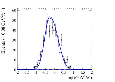
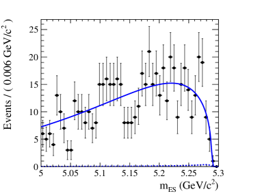
Figure 7.12: Fitted $m_{\nu}^{2}$ and $m_{\rm ES}$ distributions of the fit to OnPeak data for the electron channel.

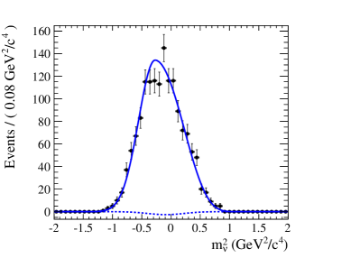
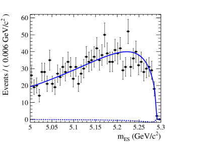
Figure 7.13: Fitted $m_{\nu}^{2}$ and $m_{\rm ES}$ distributions of the fit to OnPeak data for the muon channel.

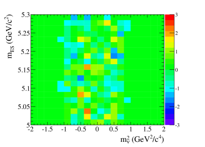
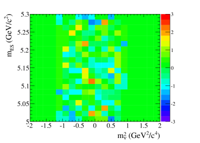
Figure 7.14: The two-dimensional pull of the fit to OnPeak data for the electron 7.14 and muon 7.14 channel.

Although the yield for $B^{-}\rightarrow\mathchar 28931\relax_{c}^{+}\overline{p}\mu^{-}\overline{\nu}_{\mu}$ is negative both yield are compatible with zero.

7.2.5 Statistical Upper Limit

The significance for both decay channels is well below the threshold for an observation, and hence we can only give an upper limit for their branching fraction. The pure statistical upper limit is obtained using a Bayesian approach by integrating the likelihood obtained in the previous section from $\mathrm{𝟎}$ to $N$, where $N$ denotes the number of signal events at which the integral coincides with $90\%$ of the integral from $\mathrm{𝟎}$ to $\infty$. The obtained upper limits for the signal yield at $90\%$ confidence level are

$$N_{\rm sig}(B^{-}\rightarrow\mathchar 28931\relax_{c}^{+}\overline{p}e^{-}\overline{\nu}_{e}) <73$$ (7.9)

$$N_{\rm sig}(B^{-}\rightarrow\mathchar 28931\relax_{c}^{+}\overline{p}\mu^{-}\overline{\nu}_{\mu}) <100.$$ (7.10)

The projection of the likelihood onto the signal yield $N_{\rm sig}$ is shown in Fig. 7.15.

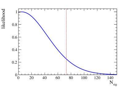
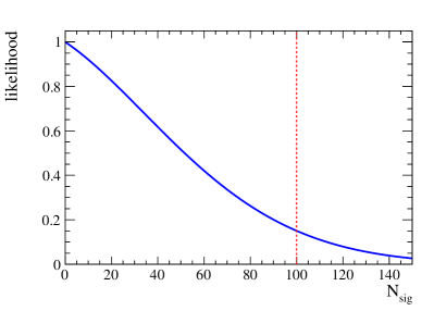
Figure 7.15: Log-likelihood projections on $N_{\rm sig}$ in OnPeak data, for the electron 7.15 and muon 7.15 channel. The dashed line shows the $90\%$ CL limit.

7.3 Efficiency calculation

We determine the reconstruction efficiency by fitting WI signal Monte Carlo with the signal and background pdfs described before. Note, that in the determination of the signal pdf only Monte Carlo events with a correctly reconstructed signal decay were used. The fitted $m_{\nu}^{2}$ and $m_{\rm ES}$ distributions, as well as the two-dimensional pull plot are shown in Fig. 7.16 and 7.17. As expected only a small background fraction is contained in signal Monte Carlo, and the agreement between Monte Carlo data and the fit function is adequate, as shown in the pull plot. From the fit we extract a signal yield of $136000\pm 600$ for the electron channel, and $127800\pm 600$ for the muon channel. Together with the number of generated events (given in Table 4.2) we obtain reconstruction efficiencies of

$$\begin{split}\epsilon(B^{-}\rightarrow\mathchar 28931\relax_{c}^{+}\overline{p}e^{-}\overline{\nu}_{e})&=(4.7422\pm 0.0021)\%\\ \epsilon(B^{-}\rightarrow\mathchar 28931\relax_{c}^{+}\overline{p}\mu^{-}\overline{\nu}_{\mu})&=(4.1248\pm 0.0020)\%.\end{split}$$ (7.11)

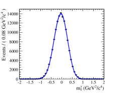
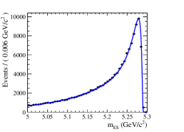
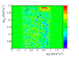
Figure 7.16: Fitted $m_{\nu}^{2}$ and $m_{\rm ES}$ distributions, as well as the two-dimensional pull of the fit to WI signal Monte Carlo data for the electron channel. The dashed line represents the signal contribution.

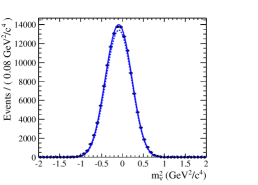
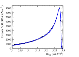
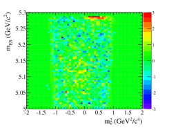
Figure 7.17: Fitted $m_{\nu}^{2}$ and $m_{\rm ES}$ distributions, as well as the two-dimensional pull of the fit to WI signal Monte Carlo data for the muon channel. The dashed line represents the signal contribution.

7.4 Systematic Uncertainties

Since the previously determined signal yields are compatible with $\mathrm{𝟎}$ the use of relative systematic uncertainties is not possible. Instead, we have to distinguish two types of systematic uncertainties and treat them separately. The first type are systematic uncertainties affecting dominantly the signal yield in OnPeak data, but represent a second order effect on the efficiency, like the used fit function. The second type of systematic uncertainties affect the reconstruction efficiency.

7.4.1 Fit function

The used fit function influences mainly the signal yield obtained in the fit to experimental data. On the efficiency the effect is expected to be small due to the negligible background contribution. Thus, we concentrate on OnPeak data for this systematic. Therefore, we decide to change the signal description in $m_{\nu}^{2}$ from a Cruijff to a Gaussian and for $m_{\rm ES}$ we leave the ARGUS shape parameter $c$ floating. The parameters of the Gaussian are

$$\mu =- 0.0477\pm 0.0010$$

$$\sigma = 0.3065\pm 0.0007$$

for the electron, and

$$\mu =- 0.0899\pm 0.0010$$

$$\sigma = 0.2963\pm 0.0007$$

for the muon channel. Fixing these parameters to the obtained values, while leaving $c$ floating we obtain

$$c =- 30\pm 12$$

$$N_{\rm sig} = 10\pm 26$$

for the electron, and

$$c =- 13\pm 15$$

$$N_{\rm sig} =- 20\pm 50$$

for the muon channel. Integrating the log-likelihood as before we obtain as upper limits for the signal yield

$$N_{\rm sig}(B^{-}\rightarrow\mathchar 28931\relax_{c}^{+}\overline{p}e^{-}\overline{\nu}_{e}) <81$$ (7.12)

$$N_{\rm sig}(B^{-}\rightarrow\mathchar 28931\relax_{c}^{+}\overline{p}\mu^{-}\overline{\nu}_{\mu}) <130.$$ (7.13)

We decide to use these values for the upper limit, rather than those obtained in section 7.2.5, as a conservative limit.

7.4.2 $B$ counting, tracking and particle identification

Three standard sources of systematic uncertainties are the $B$ counting, the charged track reconstruction and the particle identification. The uncertainty from the $B$ counting can be directly taken from the number of $B\kern 1.79993pt\overline{\kern-1.79993ptB}{}$ pairs, given in eq. (4.4), and accounts for an uncertainty of $0.6\%$.

The tracking uncertainty is given by the tracking group [46], and amounts to a relative uncertainty of $0.128\%$ per track for the used tracking list Charged Tracks. Adding up these uncertainties in quadrature leads to an overall tracking uncertainty of $0.3\%$.

For the uncertainty from particle identification we take advantage of the correction tables applied to Monte Carlo events. These correction tables try to balance the differences between data and Monte Carlo events. A standard method to obtain the systematic uncertainties is to turn off these correction tables and compare the number of reconstructed events with each other. The difference in these numbers can be taken as systematic uncertainty from particle identification. With the correction tables enabled, we obtain signal yields of

$$N_{\rm sig}(B^{-}\rightarrow\mathchar 28931\relax_{c}^{+}\overline{p}e^{-}\overline{\nu}_{e}) =136000\pm 600,$$ (7.14)

$$N_{\rm sig}(B^{-}\rightarrow\mathchar 28931\relax_{c}^{+}\overline{p}\mu^{-}\overline{\nu}_{\mu}) =127800\pm 600$$ (7.15)

on WI signal Monte Carlo, as described in section 7.3 for the efficiency calculation. Repeating this fit on WI signal Monte Carlo events without the correction tables return signal yields of

$$N_{\rm sig}(B^{-}\rightarrow\mathchar 28931\relax_{c}^{+}\overline{p}e^{-}\overline{\nu}_{e}) =141800\pm 600,$$ (7.16)

$$N_{\rm sig}(B^{-}\rightarrow\mathchar 28931\relax_{c}^{+}\overline{p}\mu^{-}\overline{\nu}_{\mu}) =131500\pm 700.$$ (7.17)

The differences in the signal yield lead to systematic uncertainties of $4.3\%$ for the electron and $2.9\%$ for the muon channel. These uncertainties are mainly due to the use of the Tight particle ID lists in the $B$ and the neutrino reconstruction. While the influence on the $B$ reconstruction directly affect $m_{\nu}^{2}$ since it depends on the energy of the $Y$ system, the neutrino reconstruction affects the loose $\Delta E$ selection cut. For the latter upper limit we have to neglect this uncertainty, since it leads to a larger efficiency, and in turn would reduce the upper limit.

7.4.3 Model dependence

For the model dependence we have two possibilities, either we determine the efficiency for phase space Monte Carlo, or for a WI Monte Carlo with altered properties of the pole at threshold.

Using phase-space Monte Carlo instead of our WI model for efficiency calculation we obtain signal yields of $115300\pm 600$ for the electron and $93100\pm 600$ for the muon channel. This translates into efficiencies of $2.8\%$ and $2.2\%$, respectively. A comparison with the efficiencies given in section 7.3, this translates into systematic uncertainties of

$$u_{\rm model}(B^{-}\rightarrow\mathchar 28931\relax_{c}^{+}\overline{p}e^{-}\overline{\nu}_{e}) =41\%$$ (7.18)

$$u_{\rm model}(B^{-}\rightarrow\mathchar 28931\relax_{c}^{+}\overline{p}\mu^{-}\overline{\nu}_{\mu}) =47\%.$$ (7.19)

The fits are shown in Fig. 7.18.

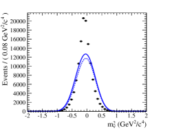
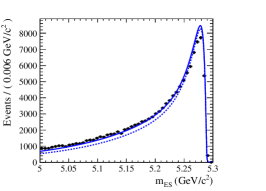
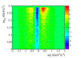
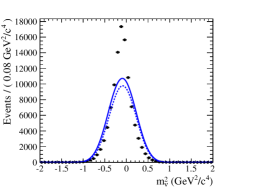
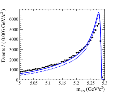
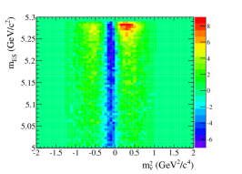
Figure 7.18: $m_{\nu}^{2}$ and $m_{\rm ES}$ projections as well as the two-dimensional pull distribution for the fit to Monte Carlo events distributed according to phase space. 7.18 for the electron and 7.18 for the muon channel.

For the second option we re-weight WI signal Monte Carlo to a threshold enhancement at the same peak position ($3.225{\mathrm{\,Ge\kern-1.00006ptV\!/}c^{2}}$), but with a doubled width of $400{\mathrm{\,Me\kern-1.00006ptV\!/}c^{2}}$. A comparison of the $200{\mathrm{\,Me\kern-1.00006ptV\!/}c^{2}}$ and $400{\mathrm{\,Me\kern-1.00006ptV\!/}c^{2}}$ broad $m(\mathchar 28931\relax_{c}^{+}\overline{p})$ enhancement on generator level is shown in Fig. 7.19.

Figure 7.19: Invariant $m(\mathchar 28931\relax_{c}^{+}\overline{p})$ mass for WI signal Monte Carlo on generator level. The black dots are the original enhancement with a width of $200{\mathrm{\,Me\kern-1.00006ptV\!/}c^{2}}$, while the blue triangles show the reweighted events with a width of $400{\mathrm{\,Me\kern-1.00006ptV\!/}c^{2}}$.

The reweighted number of generated events is $2797130$ for the electron and $3018900$ for the muon channel. To determine the analysis efficiency for these reweighted events we repeat the fit described in section 7.3. Here, we obtain a signal yield of $121600\pm 500$ for the electron channel, and $1306300\pm 600$ for the muon channel. This translates into the efficiencies

$$\epsilon_{W}(B^{-}\rightarrow\mathchar 28931\relax_{c}^{+}\overline{p}e^{-}\overline{\nu}_{e}) =4.34\%$$ (7.20)

$$\epsilon_{W}(B^{-}\rightarrow\mathchar 28931\relax_{c}^{+}\overline{p}\mu^{-}\overline{\nu}_{\mu}) =4.32\%.$$ (7.21)

Taking the difference to the non-weighted efficiencies, given in sect. 7.3, as systematic uncertainties we obtain as model-dependent systematic uncertainties

$$u_{\rm model}(B^{-}\rightarrow\mathchar 28931\relax_{c}^{+}\overline{p}e^{-}\overline{\nu}_{e}) =8.4\%$$ (7.22)

$$u_{\rm model}(B^{-}\rightarrow\mathchar 28931\relax_{c}^{+}\overline{p}\mu^{-}\overline{\nu}_{\mu}) =4.9\%.$$ (7.23)

The fitted $m_{\nu}^{2}$ and $m_{\rm ES}$ projections as well as the two-dimensional pull plots are shown in Fig. 7.20. As can be seen from the distributions the signal pdf describes the weighted signal well.

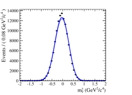
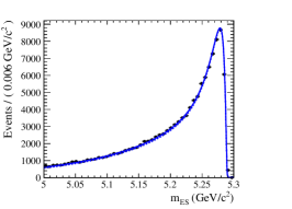
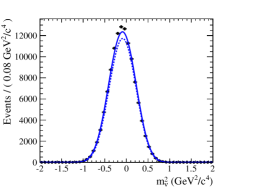
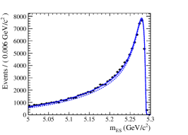
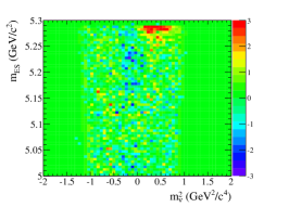
Figure 7.20: $m_{\nu}^{2}$ and $m_{\rm ES}$ projections as well as the two-dimensional pull distribution for the fit to reweighted Monte Carlo events. 7.20 for the electron and 7.20 for the muon channel.

In conclusion we have two sets of systematic uncertainties to choose from. The most conservative comes from phase space Monte Carlo, since this represents an absolute border of the model dependence. The re-weighted Monte Carlo can be seen as more realistic, but at the cost of an unknown confidence level for this uncertainty. In order to preserve a $90\%$ confidence level we decide to use the systematic uncertainties determined via phase space Monte Carlo events.

7.5 Upper Limit

With the upper limit for the signal yield, determined in sect. 7.4.1 we can determine the upper limit for the product branching fraction ${\cal B}(B^{-}\rightarrow\mathchar 28931\relax_{c}^{+}\overline{p}\ell^{-}\overline{\nu}_{\ell})\cdot{\cal B}(\mathchar 28931\relax_{c}^{+}\rightarrow pK^{-}\pi^{+})$ as

$$\frac{N_{\rm sig}}{\epsilon\cdot N_{B\kern 1.25995pt\overline{\kern-1.25995ptB}{}}},$$ (7.24)

with the efficiencies $\epsilon$, given in eq. (7.11), and the number of $B\kern 1.79993pt\overline{\kern-1.79993ptB}{}$ pairs, given in eq. (4.4). This leads to

$$\begin{split}{\cal B}(B^{-}\rightarrow\mathchar 28931\relax_{c}^{+}\overline{p}e^{-}\overline{\nu}_{e})\cdot{\cal B}(\mathchar 28931\relax_{c}^{+}\rightarrow pK^{-}\pi^{+})&<3.6\times 10^{-6}\\ {\cal B}(B^{-}\rightarrow\mathchar 28931\relax_{c}^{+}\overline{p}\mu^{-}\overline{\nu}_{\mu})\cdot{\cal B}(\mathchar 28931\relax_{c}^{+}\rightarrow pK^{-}\pi^{+})&<6.7\times 10^{-6},\end{split}$$ (7.25)

neglecting the small statistical uncertainties on the efficiency and number of $B\kern 1.79993pt\overline{\kern-1.79993ptB}{}$ pairs. These values for the upper limit are calculated at $90\%$ confidence level, but without the systematic uncertainties affecting the efficiency. Here, we only have to consider the model uncertainties which reduce the efficiency, and lead in turn to a larger upper limit. This uncertainty amounts to $41\%$ for the electron, and $47\%$ for the muon channel. Due to these large uncertainties we have to work with asymmetric error ranges and modify the efficiency with a factor $1-u_{\epsilon}$ of $0.59$ for the electron, and $0.53$ for the muon case.

$$\begin{split}{\cal B}(B^{-}\rightarrow\mathchar 28931\relax_{c}^{+}\overline{p}e^{-}\overline{\nu}_{e})\cdot{\cal B}(\mathchar 28931\relax_{c}^{+}\rightarrow pK^{-}\pi^{+})&<6.1\times 10^{-6}\\ {\cal B}(B^{-}\rightarrow\mathchar 28931\relax_{c}^{+}\overline{p}\mu^{-}\overline{\nu}_{\mu})\cdot{\cal B}(\mathchar 28931\relax_{c}^{+}\rightarrow pK^{-}\pi^{+})&<12.6\times 10^{-6}.\end{split}$$ (7.26)

Correcting for the $\mathchar 28931\relax_{c}^{+}$ branching fraction, by dividing by the world average value of $5\%$, given in [7], we obtain

$$\begin{split}{\cal B}(B^{-}\rightarrow\mathchar 28931\relax_{c}^{+}\overline{p}e^{-}\overline{\nu}_{e})\cdot\frac{{\cal B}(\mathchar 28931\relax_{c}^{+}\rightarrow pK^{-}\pi^{+})}{5\%}&<1.2\times 10^{-4}\\ {\cal B}(B^{-}\rightarrow\mathchar 28931\relax_{c}^{+}\overline{p}\mu^{-}\overline{\nu}_{\mu})\cdot\frac{{\cal B}(\mathchar 28931\relax_{c}^{+}\rightarrow pK^{-}\pi^{+})}{5\%}&<2.5\times 10^{-4}.\end{split}$$ (7.27)

We decide to use this notation, to allow for a later correction of the upper limit for a changed $\mathchar 28931\relax_{c}^{+}$ branching fraction, since the current value has a large model-dependent uncertainty. If we would take the recent Belle measurement on the $\mathchar 28931\relax_{c}^{+}$ branching fraction [47],

$${\cal B}(\mathchar 28931\relax_{c}^{+}\rightarrow pK^{-}\pi^{+})=(6.84\pm 0.24^{+0.21}_{-0.27})\%$$ (7.28)

the upper limits would be

$$\begin{split}{\cal B}(B^{-}\rightarrow\mathchar 28931\relax_{c}^{+}\overline{p}e^{-}\overline{\nu}_{e})\cdot\frac{{\cal B}(\mathchar 28931\relax_{c}^{+}\rightarrow pK^{-}\pi^{+})}{6.84\%}&<0.9\times 10^{-4}\\ {\cal B}(B^{-}\rightarrow\mathchar 28931\relax_{c}^{+}\overline{p}\mu^{-}\overline{\nu}_{\mu})\cdot\frac{{\cal B}(\mathchar 28931\relax_{c}^{+}\rightarrow pK^{-}\pi^{+})}{6.84\%}&<1.8\times 10^{-4}.\end{split}$$ (7.29)

For the combined upper limit for $B^{-}\rightarrow\mathchar 28931\relax_{c}^{+}\overline{p}\ell^{-}\overline{\nu}_{\ell}$ we perform a simultaneous, unbinned maximum likelihood fit in $m_{\rm ES}$ and $m_{\nu}^{2}$ for the electron and the muon channel. The common variable is the efficiency corrected signal yield. For the fit we use the same functions as in section 7.4.1, where we determined the systematic uncertainty arising from the used fit function. Here, we fix all parameters to the obtained values in section 7.4.1. For the efficiency correction of the signal yields we use the values given in eq. (7.11). The $m_{\rm ES}$ and $m_{\nu}^{2}$ projections for both decay modes are shown in Fig. 7.21.

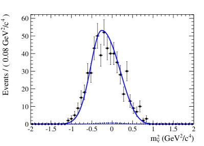
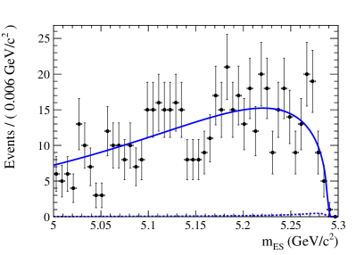
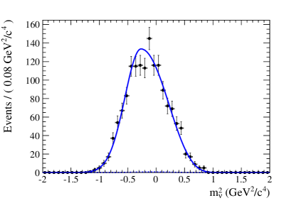
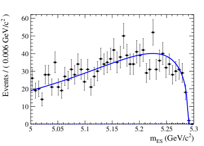
Figure 7.21: Fit projections for the electron (7.21, 7.21) and muon (7.21, 7.21) channel from the simultaneous fit. The dashed line shows the signal component.

The likelihood in dependence of the signal yield is shown in Fig. 7.22. The Bayesian upper limit for the signal yield at $90\%$ confidence level is $1279$ events.

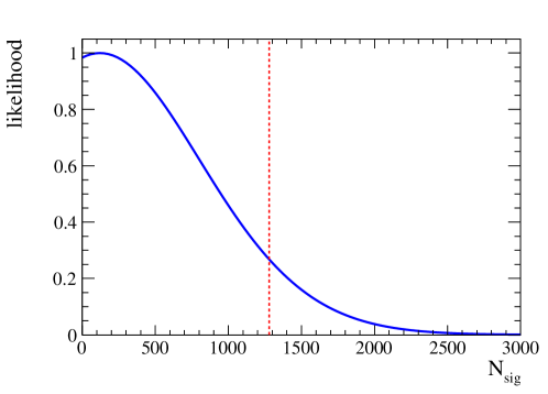
Figure 7.22: Likelihood for the simultaneous fit for the electron and the muon channel.

With the number of $B\kern 1.79993pt\overline{\kern-1.79993ptB}{}$ pairs, given in eq. (4.4), this translates into

$${\cal B}(B^{-}\rightarrow\mathchar 28931\relax_{c}^{+}\overline{p}\ell^{-}\overline{\nu}_{\ell})\cdot{\cal B}(\mathchar 28931\relax_{c}^{+}\rightarrow pK^{-}\pi^{+}) <2.7\times 10^{-6}.$$ (7.30)

For the systematic uncertainty arising from the model dependence of the efficiency we take the average of the correction factors given in the previous section, which is $0.56$, and obtain after the correction for the $\mathchar 28931\relax_{c}^{+}$ branching fraction an upper limit of

$${\cal B}(B^{-}\rightarrow\mathchar 28931\relax_{c}^{+}\overline{p}\ell^{-}\overline{\nu}_{\ell})\cdot\frac{{\cal B}(\mathchar 28931\relax_{c}^{+}\rightarrow pK^{-}\pi^{+})}{5\%} <1.0\times 10^{-4},$$ (7.31)

for the world average value of $5\%$ for ${\cal B}(\mathchar 28931\relax_{c}^{+}\rightarrow pK^{-}\pi^{+})$, and for the recent Belle result of $6.84\%$ an upper limit of

$${\cal B}(B^{-}\rightarrow\mathchar 28931\relax_{c}^{+}\overline{p}\ell^{-}\overline{\nu}_{\ell})\cdot\frac{{\cal B}(\mathchar 28931\relax_{c}^{+}\rightarrow pK^{-}\pi^{+})}{6.84\%} <0.7\times 10^{-4}.$$ (7.32)

Chapter 8 Conclusion

The present analysis is a search for the semi-leptonic $B$ decay $B^{-}\rightarrow\mathchar 28931\relax_{c}^{+}\overline{p}\ell^{-}\overline{\nu}_{\ell}$. Neither for the electron, nor the muon mode a signal could be established. This led to the $90\%$ CL upper limits of

$$\begin{split}{\cal B}(B^{-}\rightarrow\mathchar 28931\relax_{c}^{+}\overline{p}e^{-}\overline{\nu}_{e})\cdot\frac{{\cal B}(\mathchar 28931\relax_{c}^{+}\rightarrow pK^{-}\pi^{+})}{5\%}&<1.2\times 10^{-4},\\ {\cal B}(B^{-}\rightarrow\mathchar 28931\relax_{c}^{+}\overline{p}\mu^{-}\overline{\nu}_{\mu})\cdot\frac{{\cal B}(\mathchar 28931\relax_{c}^{+}\rightarrow pK^{-}\pi^{+})}{5\%}&<2.5\times 10^{-4},\\ {\cal B}(B^{-}\rightarrow\mathchar 28931\relax_{c}^{+}\overline{p}\ell^{-}\overline{\nu}_{\ell})\cdot\frac{{\cal B}(\mathchar 28931\relax_{c}^{+}\rightarrow pK^{-}\pi^{+})}{5\%}&<1.0\times 10^{-4}.\end{split}$$ (8.1)

All three limits are in a slight tension with two of the predictions given in sect. 2.3, which are of the order $5\times 10^{-4}$. There are three possible explanations for this tension:

1. An unknown suppression factor reduces this branching fraction.

2. The predictions in sect. 2.3 rely on inaccurate assumptions.

3. The decay model used in this analysis for signal simulation is not accurate.

Although the first one is the most interesting one, it is the most unlikely explanation as well. For the second explanation we have to take a closer look on the two predictions again. The first one is derived from the branching fraction for $B^{-}\rightarrow p\overline{p}\ell^{-}\overline{\nu}_{\ell}$ by assuming a simple CKM suppression between the two decays. This ignores completely the different size of the available phase space, as well as different form factors for the fragmentation into the hadronic part of the final state. These form factors can depend on the invariant mass of the final state particles, and thus might affect the prediction substantially. The second prediction comes from the decay $B^{-}\rightarrow\mathchar 28931\relax_{c}^{+}\overline{p}\pi^{-}$, assuming that $100\%$ of this decay proceeds via the external $W$ Feynman graph, which is probably not accurate. A possible solution for this problem comes from the isospin analysis given in [20], where the contribution of the external graph is determined based on simple isospin arguments. The upper limit we obtained here is compatible with the predicted limit in [20] and might corroborate the isospin argumentation. Last but not least, we have to consider the used Monte Carlo model in this analysis. We modelled the semi-leptonic decay according to the weak matrix element, assuming a meson-like pole near threshold decaying into $\mathchar 28931\relax_{c}^{+}\overline{p}$. Despite being well motivated from the analysis of full hadronic baryonic $B$-decays this pole model might prove to be wrong. Another factor here might be the quark hadron duality, since the weak matrix element is only valid on quark-level, neglecting the influence of the hadronization.

On the experimental side the analysis suffered from the high mass of the final state particles, rendering the classical signal variables used in semi-leptonic $B$ decays useless, as was shown in sect. 7.1.1. A similar problem was already observed in the analysis of $B^{-}\rightarrow D_{s}^{+}K^{-}\ell^{-}\overline{\nu}_{\ell}$ [44]. To circumvent this problem, a tagged analysis approach, where the second $B$ is fully reconstructed in a pure hadronic mode, is advisable. Belle II, which will have a multitude of the BABAR dataset available for analysis, should be able to perform a tagged search for the decay $B^{-}\rightarrow\mathchar 28931\relax_{c}^{+}\overline{p}\ell^{-}\overline{\nu}_{\ell}$. LHCb should be able to study this decay mode as well. The large boost and the resulting displaced vertex could enable them to obtain a rather clean signal for $B^{-}\rightarrow\mathchar 28931\relax_{c}^{+}\overline{p}\mu^{-}\overline{\nu}_{\mu}$ without the need for a neutrino reconstruction.

The measurement of the semileptonic decay $B^{-}\rightarrow\mathchar 28931\relax_{c}^{+}\overline{p}\ell^{-}\overline{\nu}_{\ell}$ stays crucial for the understanding of baryonic $B$-decays. A direct observation will enable us to quantify the impact of the external Feynman graph on the overall branching fraction of fully hadronic baryonic $B$ decays. In addition, it will provide valuable insight on the threshold enhancement described in sect. 2.2, especially on the absence of such an enhancement in the decay $\kern 1.79993pt\overline{\kern-1.79993ptB}{}^{0}\rightarrow\mathchar 28934\relax_{c}(2455)^{0}\overline{p}\pi^{-}$. Consequently it will help to decide if the model given in [16] is correct.

Appendix A Random Forest input variables

A.1 $q\overline{q}$ random forest

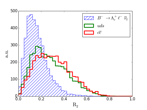
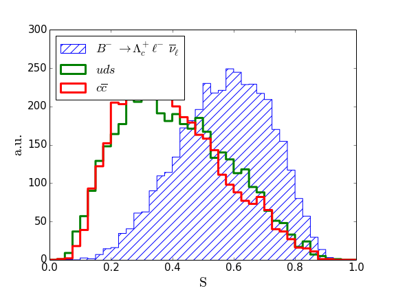
Figure A.1: Comparison of WI signal Monte Carlo (blue histogram) and $q\overline{q}$ background Monte Carlo (green and red lines) for the three Random Forest input variables, A.1 $R_{2}$, A.1 $S$, and A.1 $cos\Delta\theta_{\rm thrust}$.

A.2 $B{\kern-1.60004pt\kern 1.79993pt\overline{\kern-1.79993ptB}{}}$ random forest

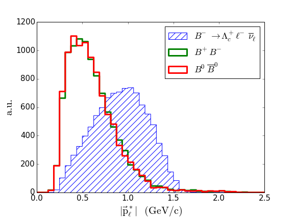
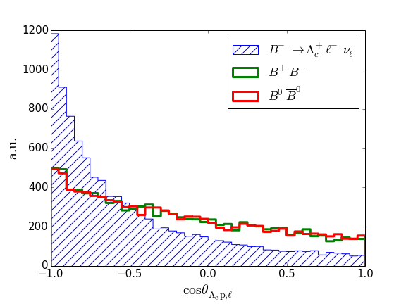
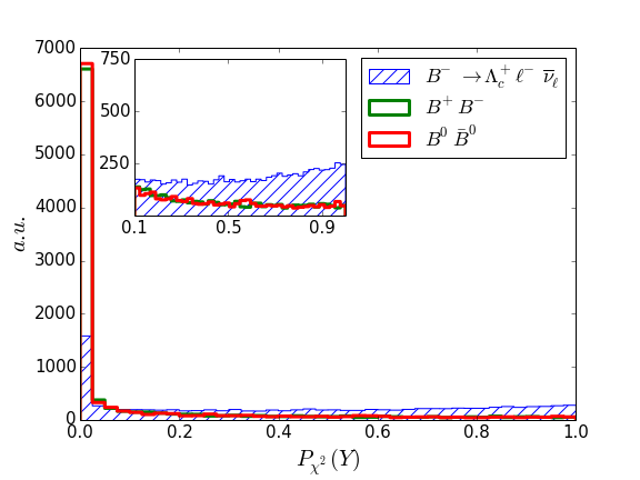
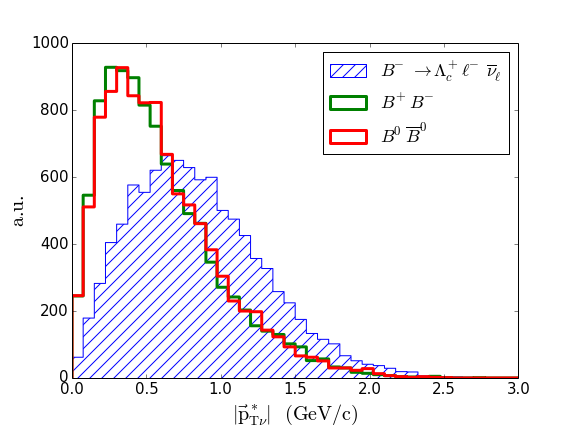
Figure A.2: Comparison of WI signal simulation events and generic $B$ decays. A.2 $|\vec{p}_{\ell}^{*}|$, A.2 $\cos\theta_{\mathchar 28931\relax_{c}p,\ell}$, A.2 $P_{\chi^{2}}(Y)$, and A.2 $p_{T\nu}$.

Appendix B Muon Channel target variables

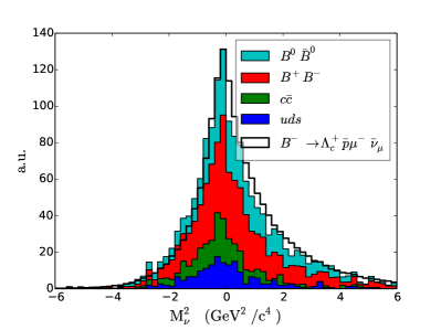
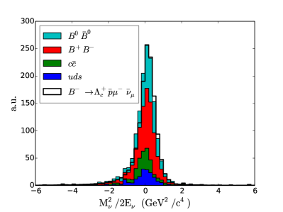
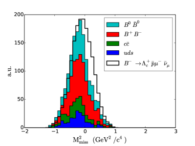
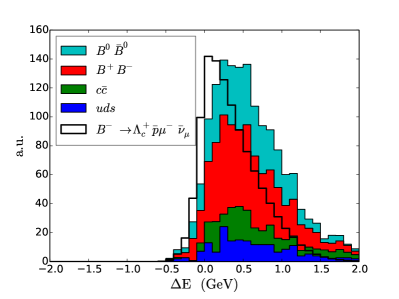
Figure B.1: Comparison of WI signal Monte Carlo and generic background Monte Carlo for B.1 $M_{\nu}^{2}$, B.1 $M_{\nu}^{2}/E_{\nu}$, B.1 $M_{\rm miss}^{2}$, andB.1 $\Delta E$. The background Monte Carlo is scaled to OnPeak luminosity and stacked. The WI Monte Carlo is scaled to match the height of the background peak.

Appendix C Fit procedure

C.1 Correlation checks

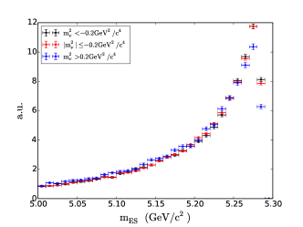
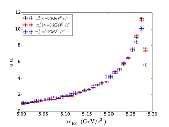
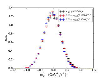
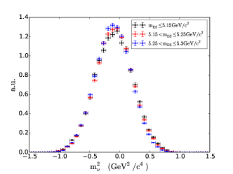
Figure C.1: $m_{\rm ES}$ and $m_{\nu}^{2}$ in slices of each other. On the left hand side for electron, and on the right hand side for muon WI signal Monte Carlo events.

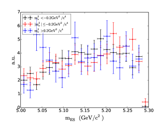
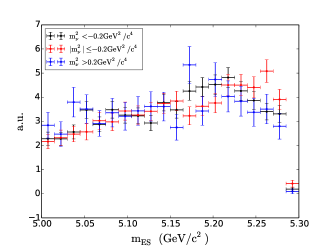
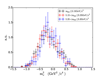
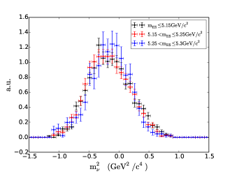
Figure C.2: $m_{\rm ES}$ and $m_{\nu}^{2}$ in slices of each other. On the left hand side for electron, and on the right hand side for muon background Monte Carlo events.

C.2 Fit validation

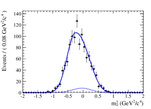
(a) 100 signal events

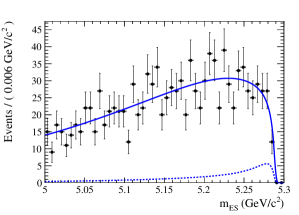
(b) 100 signal events

(c) 50 signal events

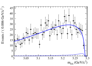
(d) 50 signal events

(e) 10 signal events

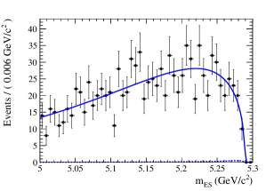
(f) 10 signal events

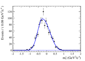
(g) 0 signal events

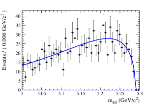
(h) 0 signal events

Figure C.3: $m_{\nu}^{2}$ and $m_{\rm ES}$ projections for the fit validation for the electron channel. Shown are the fits for $100,50,10$ and $\mathrm{𝟎}$ input signal events.

(a) 100 signal events

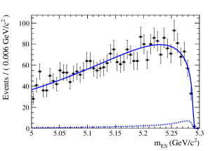
(b) 100 signal events

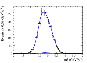
(c) 50 signal events

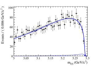
(d) 50 signal events

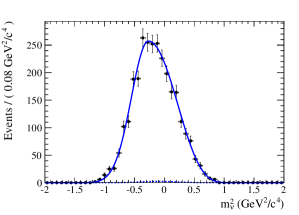
(e) 10 signal events

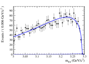
(f) 10 signal events

(g) 0 signal events

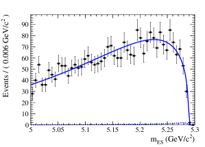
(h) 0 signal events

Figure C.4: $m_{\nu}^{2}$ and $m_{\rm ES}$ projections for the fit validation for the muon channel. Shown are the fits for $100,50,10$ and $\mathrm{𝟎}$ input signal events.

References

- [1] Yao, W.-M., Particle Physics Booklet. Institute of Physics Publishing, July, 2006.
- [2] BABAR Collaboration, B. Aubert et al., “Measurements of and and Studies of Resonances,” Phys.Rev. D78 (2008) 112003, arXiv:0807.4974 [hep-ex].
- [3] BABAR Collaboration, B. Aubert et al., “Measurement of the branching fraction and polarization in ,” Phys. Rev. D 79 (2009) 112009. http://link.aps.org/doi/10.1103/PhysRevD.79.112009.
- [4] BABAR Collaboration, B. Aubert et al., “Observation of the baryonic -decay ,” Phys. Rev. D 80 (2009) 051105. http://link.aps.org/doi/10.1103/PhysRevD.80.051105.
- [5] M. Ebert, “Baryonic decays at BABAR.” Pos (eps-hep 2009)215, 2009.
- [6] BABAR Collaboration, P. del Amo Sanchez et al., “Observation and study of the baryonic -meson decays ,” Phys. Rev. D 85 (2012) 092017. http://link.aps.org/doi/10.1103/PhysRevD.85.092017.
- [7] Particle Data Group Collaboration, J. Beringer et al., “Review of Particle Physics,” Phys.Rev. D86 (2012) 010001.
- [8] BABAR Collaboration, e. Harrison, P. F. and e. Quinn, Helen R., “The BABAR physics book: Physics at an asymmetric B factory,”. Papers from Workshop on Physics at an Asymmetric B Factory (BABAR Collaboration Meeting), Rome, Italy, 11-14 Nov 1996, Princeton, NJ, 17-20 Mar 1997, Orsay, France, 16-19 Jun 1997 and Pasadena, CA, 22-24 Sep 1997.
- [9] ARGUS Collaboration, H. Albrecht et al., “Measurement of inclusive baryon production in B meson decays,” Z.Phys. C56 (1992) 1–6.
- [10] T. Leddig, “Measurement of the Branching Fraction with the BABAR Detector,” 2009. Diplomarbeit, University of Rostock.
- [11] Wikipedia, “Quantum electrodynamics,” March, 2008. {http://en.wikipedia.org/wiki/Quantum_electrodynamics}.
- [12] BELLE Collaboration Collaboration, S. Choi et al., “Observation of a resonance-like structure in the mass distribution in exclusive decays,” Phys.Rev.Lett. 100 (2008) 142001, arXiv:0708.1790 [hep-ex].
- [13] LHCb collaboration Collaboration, R. Aaij et al., “Observation of the resonant character of the state,” Phys.Rev.Lett. 112 (2014) 222002, arXiv:1404.1903 [hep-ex].
- [14] M. Suzuki, “Partial waves of baryon-antibaryon in three-body B meson decay,” Journal of Physics G: Nuclear and Particle Physics 34 (2007) no. 2, 283. http://stacks.iop.org/0954-3899/34/i=2/a=009.
- [15] J. L. Rosner, “Low mass baryon anti-baryon enhancements in B decays,” Phys.Rev. D68 (2003) 014004, arXiv:hep-ph/0303079 [hep-ph].
- [16] T. Hartmann, Study of the decay and its intermediate states. Mensch & Buch Verl, Berlin, 2011.
- [17] CLEO Collaboration Collaboration, G. Bonvicini et al., “Study of semileptonic decays of B mesons to charmed baryons,” Phys.Rev. D57 (1998) 6604–6608, arXiv:hep-ex/9712008 [hep-ex].
- [18] BaBar Collaboration Collaboration, J. Lees et al., “Search for Decays in Events With a Fully Reconstructed B Meson,” Phys.Rev. D85 (2012) 011102, arXiv:1110.6005 [hep-ex].
- [19] Collaboration M. Z. Wang for the Belle Collaboration, K. Tien et al., “Evidence for Semileptonic Decays,” arXiv:1306.3353 [hep-ex].
- [20] M. Ebert, Isospin analysis and study of the decay modes and . Mensch & Buch Verl, Berlin, 2012.
- [21] BABAR Collaboration, Aubert, B. et al., “The BABAR detector,” Nucl. Instrum. Meth. A479 (2002) 1–116.
- [22] BABAR Collaboration, D. e. a. Boutigny, “BABAR technical design report,”. SLAC-R-0457.
- [23] A. J. Hart, Investigation of the Charmless Decay using a Dalitz Plot Analysis at BABAR. PhD thesis, University of Bermingham, 2006.
- [24] Re, V. et al., “The BABAR Silicon Vertex Tracker: performance and radiation damage studies,” Nucl. Instrum. Meth. A530 (2004) 7–11.
- [25] BABAR Collaboration, Kelsey, Michael H., “Performance and aging of the BABAR drift chamber,” Nucl. Instrum. Meth. A535 (2004) 206–211.
- [26] BABAR-DIRC Collaboration, Adam, I. et al., “The DIRC particle identification system for the BABAR experiment,” Nucl. Instrum. Meth. A538 (2005) 281–357.
- [27] A. Ruland, “Performance and operation of the BaBar calorimeter,” J.Phys.Conf.Ser. 160 (2009) 012004.
- [28] BABAR Collaboration, B. Aubert et al., “The BABAR Detector: Upgrades, Operation and Performance,” Nucl.Instrum.Meth. A729 (2013) 615–701, arXiv:1305.3560 [physics.ins-det].
- [29] BABAR trigger group, “What is the BABAR trigger,” August, 2008. {http://www.slac.stanford.edu/BFROOT/www/Detector/Trigger/trigger_whatsit.html}.
- [30] BABAR Neutrals AWG, “Neutral-Particle Reconstruction,” August, 2013. {https://bbr-wiki.slac.stanford.edu/bbr_wiki/index.php/Physics/Neutrals}.
- [31] BABAR Tracking AWG, “New BtaCandidate Lists,” August, 2013. {http://www.slac.stanford.edu/BFROOT/www/Physics/Charged.html#Lists}.
- [32] BABAR PID group, “Decision trees in particle identification,” 2013. {https://bbr-wiki.slac.stanford.edu/bbr_wiki/index.php/Physics/PID/Decision_trees_in_PID}.
- [33] I. Narsky, “Optimization of signal significance by bagging decision trees,” arXiv:physics/0507157 [physics].
- [34] C. O. Vuosalo and others, “Muon Identification Using Decision Trees.” BABAR analysis document 1853.
- [35] P. Ongmongkolkul and others, “Particle Identification Using Error Correcting Output Code Multiclass Classifier.” BABAR analysis document 2199.
- [36] “The ROOT system homepage.” {http://root.cern.ch}.
- [37] “iPython.” {http://www.ipython.org/}.
- [38] “SciPy.org.” {http://www.scipy.org/}.
- [39] Hastie, T. and Tibshirani, R. and Friedmann, J., The Elements of Statistical Learning. Springer Verlag, 2008.
- [40] D. J. Lange, “The EvtGen particle decay simulation package,” Nucl. Instrum. Meth. A462 (2001) 152–155.
- [41] GEANT4 Collaboration, S. Agostinelli et al., “GEANT4: A simulation toolkit,” Nucl. Instrum. Meth. A506 (2003) 250–303.
- [42] BABAR Collaboration, B. Aubert et al., “Precision measurement of the baryon mass,” Phys. Rev. D 72 (2005) 052006.
- [43] T. Sjostrand, S. Mrenna, and P. Z. Skands, “PYTHIA 6.4 Physics and Manual,” JHEP 0605 (2006) 026, arXiv:hep-ph/0603175 [hep-ph].
- [44] H. Jasper, “Search for the semileptonic decay .” BABAR analysis document 2183.
- [45] ARGUS Collaboration, Albrecht, H. and others, “Exclusive hadronic decays of mesons,” Z. Phys. C48 (1990) 543–552.
- [46] BABAR tracking group, “Tracking Efficiency Task Force,” 2010. {http://www.slac.stanford.edu/BFROOT/www/Physics/TrackEfficTaskForce/TauEff/R24/TauEff.html}.
- [47] Belle Collaboration Collaboration, A. Zupanc et al., “Measurement of the Branching Fraction ,” Phys.Rev.Lett. 113 (2014) 042002, arXiv:1312.7826 [hep-ex].
- [48] T. Hartmann, “Messung des Verzweigungsverhältnisses von ,” Diplomarbeit, Universität Rostock, 2006.
- [49] R. Nogowski, Precision Measurement of the Mass Difference of Neutral and Charged B Mesons. PhD thesis, Technische Universiät Dresden, 2007.
- [50] H. Schröder, R. Waldi, M. Ebert, T. Hartmann, “ Decays to Baryons.” BABAR analysis document 2032.
- [51] J. Dingfelder, M. Kelsey, V. Lüth, W. Wulsin, “Study of Charmless Semileptonic Decays and with Neutrino Reconstruction.” BABAR analysis document 1520.
- [52] A. J. Bevan, “Multivariate Analysis Notes.”.
- [53] A. Ali, “ Decays - Introduction and Overview,” in Decays. World Scientific, 1994.
- [54] D. Griffiths, Einführung in die Elementarteilchenphysik. Akademie Verlag, 1996.
- [55] Marcus Ebert, “EMC information for the Proton LH-selector,” 2006. BABAR analysis document 1352.
- [56] S.A. Majewski, “Study of the Decays and ,” 2008. BABAR analysis document 1670 Version 8.
- [57] M. Ebert, “Study of ,” 2008. BABAR analysis document 1691.
- [58] W. Dunwoodie, “Simple Observations on Kinematics,” 2002. {http://www.slac.stanford.edu/~wmd/bbkinematics/kinematics.note.gz}.
- [59] W. Dunwoodie, “Suggestion for the Parametrization of Dalitz Plot Efficiency,” 2004. {http://www.slac.stanford.edu/~wmd/bbkinematics/dalitz_efficiency.note.gz}.
-
[60]
BABAR Charged Particle AWG, “A short description of the LH selectors,”
2002.
{http://www.slac.stanford.edu/BFROOT/www/Physics/Tools/Pid/Hadrons/
Description_of_the_LH_selectors.html}. - [61] BABAR Collaboration, P. del Amo Sanchez et al., “Study of and decays and determination of ,” Phys.Rev. D83 (2011) 032007.
- [62] Belle Collaboration, N. Gabyshev et al., “Observation of decay,” Phys.Rev.Lett. 90 (2003) 121802, arXiv:hep-ex/0212052 [hep-ex].
- [63] BABAR Collaboration, B. Aubert et al., “Observation of the decay ,” Phys.Rev. D82 (2010) 031102, arXiv:1007.1370 [hep-ex].
- [64] Belle Collaboration, N. Gabyshev et al., “Study of decay mechanisms in decays and observation of low-mass structure in the system,” Phys.Rev.Lett. 97 (2006) 242001, arXiv:hep-ex/0409005 [hep-ex].
- [65] H.-Y. Cheng and K.-C. Yang, “Charmless exclusive baryonic B decays,” Phys.Rev. D66 (2002) 014020, arXiv:hep-ph/0112245 [hep-ph].
- [66] T. Leddig, “Study of ,” 2009. BABAR analysis document 2149, Version 8.
- [67] T. Sjostrand, “PYTHIA 5.7 and JETSET 7.4: Physics and manual,” arXiv:hep-ph/9508391 [hep-ph].
- [68] C. Q. Geng and Y. K. Hsiao, “Determination of nucleon form factors from baryonic decays,” Phys. Rev. D 75 (2007) 094005. http://link.aps.org/doi/10.1103/PhysRevD.75.094005.
- [69] G. Punzi, “Sensitivity of searches for new signals and its optimization,” arXiv:physics/0308063v2 [physics].