Layered Adaptive Importance Sampling

Abstract

Monte Carlo methods represent the de facto standard for approximating complicated integrals involving multidimensional target distributions. In order to generate random realizations from the target distribution, Monte Carlo techniques use simpler proposal probability densities to draw candidate samples. The performance of any such method is strictly related to the specification of the proposal distribution, such that unfortunate choices easily wreak havoc on the resulting estimators. In this work, we introduce a layered (i.e., hierarchical) procedure to generate samples employed within a Monte Carlo scheme. This approach ensures that an appropriate equivalent proposal density is always obtained automatically (thus eliminating the risk of a catastrophic performance), although at the expense of a moderate increase in the complexity. Furthermore, we provide a general unified importance sampling (IS) framework, where multiple proposal densities are employed and several IS schemes are introduced by applying the so-called deterministic mixture approach. Finally, given these schemes, we also propose a novel class of adaptive importance samplers using a population of proposals, where the adaptation is driven by independent parallel or interacting Markov Chain Monte Carlo (MCMC) chains. The resulting algorithms efficiently combine the benefits of both IS and MCMC methods.
Keywords: Bayesian Inference; Adaptive Importance Sampling; Population Monte Carlo; parallel MCMC

1 Introduction

Monte Carlo methods currently represent a maturing toolkit widely used throughout science and technology (Doucet:MCSignalProcessing2005, ; Robert04, ; Wang:MCWirelessComm2002, ). Importance sampling (IS) and Markov Chain Monte Carlo (MCMC) methods are well-known Monte Carlo (MC) techniques applied to compute integrals involving a high-dimensional target probability density function (pdf) $\bar{\pi}({\bf x})$. In both cases, the choice of a suitable proposal density $q({\bf x})$ is crucial for the success of the Monte Carlo based approximation. For this reason, the design of adaptive IS or MCMC schemes represents one of the most active research topics in this area, and several methods have been proposed in the literature (Cappe04, ; CORNUET12, ; Craiu09, ; Haario2001, ; Luengo13, ).

Since both IS and MCMC have certain intrinsic advantages and weaknesses, several attempts have been made to successfully marry the two approaches, producing hybrid techniques: IS-within-MCMC (Andrieu10, ; Brockwell10, ; Liesenfeld08, ; Liu00, ; Neal11, ) or MCMC-within-IS (Beaujean13, ; Botev13, ; Chopin02, ; EBEB14, ; Mendes15, ; Neal01, ; Yuan13, ). To set the scene for such developments it is useful to recall briefly some of the main strengths of IS and MCMC, respectively. For instance, one benefit of IS is that it delivers a straightforward estimate of the normalizing constant of $\bar{\pi}({\bf x})$ (Liang10, ; Robert04, ) (a.k.a. evidence or marginal likelihood), which is essential for several applications (FRIEL11, ; Skilling06, ). In contrast, the estimation of the normalizing constant is highly challenging using MCMC methods, and several authors have investigated different approaches to overcome the obstacles related to the instability of the resulting estimators (Botev08, ; CALDWELL14, ; Chib01, ; FRIEL11, ; Weinberg10, ). Furthermore, the application and the theoretical analysis of an IS scheme using an adaptive proposal pdf is easier than the theoretical analysis of the corresponding adaptive MCMC scheme, which is much more delicate (Andrieu08, ).

On the other hand, an appealing feature of MCMC algorithms is their explorative behavior. For instance, the proposal function $q({\bf x}|{\bf x}_{t-1})$ can depend on the previous state of the chain ${\bf x}_{t-1}$ and foster movements between different regions of the target density. For this reason, MCMC methods are usually preferred when no detailed information about the target $\bar{\pi}({\bf x})$ is available, especially in large dimensional spaces (Andrieu:MCMachineLearning2003, ; Fitzgerald01, ). Moreover, in order to amplify their explorative behavior several parallel MCMC chains can be run simultaneously (Robert04, ; Liang10, ). This strategy facilitates the exploration of the state space, although at the expense of an increase in the computational cost. Several schemes have been introduced to share information among the different chains (Craiu09, ; O-MCMC, ; Smelly, ), which further improves the overall convergence.

The main contribution of this work is the description and analysis of a hierarchical proposal procedure for generating samples, which can then be employed within any Monte Carlo algorithm. In this hierarchical scheme, we consider two conditionally independent levels: the upper level is used to generate mean vectors for the proposal pdfs, which are then used in the lower level to draw candidate samples according to some MC scheme. We show that the standard Population Monte Carlo (PMC) method (Cappe04, ) can be interpreted as applying implicitly this hierarchical procedure.

The second major contribution of this work is providing a general framework for multiple importance sampling (MIS) schemes and their iterative adaptive versions. We discuss several alternative applications of the so-called deterministic approach (ElviraMIS15, ; Owen00, ; Veach95, ) for sampling a mixture of pdfs. This general framework includes different MIS schemes used within adaptive importance sampling (AIS) techniques already proposed in literature, such as the standard PMC (Cappe04, ), the adaptive multiple importance sampling (AMIS) (CORNUET12, ; Marin12, ), and the adaptive population importance sampling (APIS) (APIS15, ).

Finally, we combine the general MIS framework with the hierarchical procedure for generating samples, introducing a new class of AIS algorithms. More specifically, one or several MCMC chains are used for driving an underlying MIS scheme. Each algorithm differs from the others in the specific Markov adaptation employed and the particular MIS technique applied for yielding the final Monte Carlo estimators. This novel class of algorithms efficiently combines the main strengths of the IS and the MCMC methods, since it maintains an explorative behavior (as in MCMC) and can still easily estimate the normalizing constant (as in IS).

We describe in detail the simplest possible algorithm of this class, called random walk importance sampling. Moreover, we introduce two additional population-based variants that provide a good trade-off between performance and computational cost. In the first variant, the mean vectors are updated according to independent parallel MCMC chains. In the other one, an interacting adaptive strategy is applied. In both cases, all the adapted proposal pdfs collaborate to yield a single global IS estimator. One of the proposed algorithms, called parallel interacting Markov adaptive importance sampling (PI-MAIS), can be interpreted as parallel MCMC chains cooperating to produce a single global estimator, since the chains exchange statistical information to achieve a common purpose.

The rest of the paper is organized as follows. Section 2 is devoted to the problem statement. The hierarchical proposal procedure is then introduced in Section 3. In Section 4, we describe a general framework for importance sampling schemes using a population of proposal pdfs, whereas Section 5 introduces the adaptation procedure for the mean vectors of these proposal pdfs. Numerical examples are provided in Section 6, including comparisons with several benchmark techniques. Different scenarios have been considered: a multimodal distribution, a nonlinear banana-shaped target, a high-dimensional example, and a localization problem in a wireless sensor network. Finally, Section 7 contains some brief final remarks.

2 Target distribution and related integrals

In this work, we focus on the Bayesian applications of IS and MCMC. However, the algorithms described may also be used for approximating any target distribution that needs to be handled by simulation methods. Let us denote the variable of interest as ${\bf x}\in\mathcal{X}\subseteq\mathbb{R}^{D_{x}}$, and let ${\bf y}\in\mathbb{R}^{D_{y}}$ be the observed data. The posterior pdf is then given by

$$\bar{\pi}({\bf x})=p({\bf x}|{\bf y})=\frac{\ell({\bf y}|{\bf x})g({\bf x})}{Z({\bf y})},$$ (1)

where $\ell({\bf y}|{\bf x})$ is the likelihood function, $g({\bf x})$ is the prior pdf, and $Z({\bf y})$ is the model evidence or partition function. In general, $Z({\bf y})$ is unknown, so we consider the corresponding unnormalized target,

$$\pi({\bf x})=\ell({\bf y}|{\bf x})g({\bf x}).$$ (2)

Our goal is computing efficiently some integral measure w.r.t. the target pdf,

$$I=\frac{1}{Z}\int_{\mathcal{X}}f({\bf x})\pi({\bf x})d{\bf x},$$ (3)

where

$$Z=\int_{\mathcal{X}}\pi({\bf x})d{\bf x},$$ (4)

and $f$ is any square-integrable function (w.r.t. $\bar{\pi}({\bf x})$) of ${\bf x}$. In this work, we address the problem of approximating $I$ and $Z$ via Monte Carlo methods. Since drawing directly from $\bar{\pi}({\bf x})\propto\pi({\bf x})$ is impossible in many applications, Monte Carlo techniques use a simpler proposal density $q({\bf x})$ to generate random candidates, testing or weighting them according to some suitable rule. Indeed, throughout the paper we focus on the combined use of several proposal pdfs, denoted as $q_{1},\ldots,q_{J}$.

3 Hierarchical procedure for proposal generation

The performance of MC methods depends on the discrepancy between the target, $\bar{\pi}({\bf x})\propto\pi({\bf x})$, and the proposal $q({\bf x})$. Namely, the performance improves if $q({\bf x})$ is more similar (i.e., closer) to $\bar{\pi}({\bf x})$. In general, tuning the parameters of the proposal is a difficult task that requires statistical information of the target distribution. In this section, we deal with this important issue, focusing on the mean vector of the proposal pdf. More specifically, we consider a proposal pdf defined by a mean vector ${\bm{\mu}}$ and covariance matrix ${\bf C}$, denoted as $q({\bf x}|{\bm{\mu}},{\bf C})=q({\bf x}-{\bm{\mu}}|{\bf C})$. We propose the following hierarchical procedure for generating a set of samples that will be employed afterwards within some Monte Carlo technique:

1. For $j=1,\ldots,J:$

   1. Draw a mean vector ${\bm{\mu}}_{j}\sim h({\bm{\mu}})$.

   2. Draw ${\bf x}_{j}^{(m)}\sim q({\bf x}|{\bm{\mu}}_{j},{\bf C})$ for $m=1,\ldots,M$.

2. Use all the generated samples, ${\bf x}_{j}^{(m)}$ for $j=1,\ldots,J$ and $m=1,\ldots,M$, as candidates within some Monte Carlo method.

Note that $h({\bm{\mu}})$ plays the role of a prior pdf over the mean vector of $q$ in this approach. Hence, the pdf of each sample ${\bf x}_{j}^{(m)}$ can be expressed as

$$\widetilde{q}({\bf x}|{\bf C})=\int_{\mathcal{X}}q({\bf x}|{\bm{\mu}},{\bf C})h({\bm{\mu}})d{\bm{\mu}},$$ (5)

i.e., the hierarchical procedure is equivalent to drawing directly ${\bf x}_{j}^{(m)}\sim\widetilde{q}({\bf x}|{\bf C})$ for all $j=1,\ldots,J$ and $m=1,\ldots,M$. The density $\widetilde{q}$ is thus the equivalent proposal density of the whole hierarchical generating procedure. Note also that the samples ${\bm{\mu}}_{1},\ldots,{\bm{\mu}}_{J}$ are not directly used by the Monte Carlo estimator, since only the samples ${\bf x}_{j}^{(m)}$, for $j=1,\ldots,J$, $m=1,\ldots,M$, enter the actual estimator. Hence, the computational cost per iteration of this hierarchical procedure is higher than the cost of a standard approach, However, it leads to substantial computational savings in terms of improved convergence towards the target, and thus a reduced number of iterations required, as shown later in the simulations. Furthermore, note that the generation of the ${\bm{\mu}}_{j}$’s in the upper level is independent of the samples ${\bf x}_{j}^{(m)}$ drawn in the lower level, thus facilitating the theoretical analysis of the resulting algorithms, as discussed in Section 5.1.

3.1 Optimal prior $h^{*}({\bm{\mu}})$

Assuming that the parametric form of $q({\bf x}|{\bm{\mu}},{\bf C})$ and its covariance matrix ${\bf C}$ are fixed, we consider the problem of finding the optimal prior $h^{*}({\bm{\mu}}|{\bf C})$ over the mean vector ${\bm{\mu}}$. Note that, since $q({\bf x}|{\bm{\mu}},{\bf C})=q({\bf x}-{\bm{\mu}}|{\bf C})$, we can write

$$\widetilde{q}({\bf x}|{\bf C})=\int_{\mathcal{X}}q({\bf x}-{\bm{\mu}}|{\bf C})h({\bm{\mu}}|{\bf C})d{\bm{\mu}}.$$ (6)

regardless of the choice of the prior over the mean vectors in the upper level. The desirable scenario is to have the equivalent proposal $\widetilde{q}({\bf x}|{\bf C})$ coinciding exactly with the target $\bar{\pi}({\bf x})$, i.e.,

$$\widetilde{q}({\bf x}|{\bf C})=\int_{\mathcal{X}}q({\bf x}-{\bm{\mu}}|{\bf C})h^{*}({\bm{\mu}}|{\bf C})d{\bm{\mu}}=\bar{\pi}({\bf x}),$$ (7)

where $h^{*}({\bm{\mu}}|{\bf C})$ represents the optimal prior.

3.2 Asymptotically optimal choice of the prior $h({\bm{\mu}})$

Since Eq. (7) cannot be solved analytically in general, in this section we relax that condition and look for an equivalent proposal $\widetilde{q}$ which fulfills (7) asymptotically as $J\to\infty$. For the sake of simplicity, let us set $M=1$. Thus, we consider the generation of $J$ samples $\{{\bf x}_{1},\ldots,{\bf x}_{J}\}$, drawn using the following hierarchical procedure:

1. Draw a mean vector ${\bm{\mu}}_{j}\sim h({\bm{\mu}})$.

2. Draw ${\bf x}_{j}\sim q({\bf x}|{\bm{\mu}}_{j},{\bf C})$.

Note that we are using $J$ different proposal pdfs,

$$q({\bf x}|{\bm{\mu}}_{1},{\bf C}),\ldots,q({\bf x}|{\bm{\mu}}_{J},{\bf C}),$$

to draw $\{{\bf x}_{1},\ldots,{\bf x}_{J}\}$, with each ${\bf x}_{j}$ being drawn from the $j$-th proposal ${\bf x}_{j}\sim q({\bf x}|{\bm{\mu}}_{j},{\bf C})$. However, if the samples ${\bf x}_{1},\ldots,{\bf x}_{J}$ are used altogether regardless of their order, then it can interpreted that they have been drawn from the following mixture using the deterministic mixture sampling scheme (see (mcbookOwen, , Chapter 9), ElviraMIS15 ):

$$\psi({\bf x})=\frac{1}{J}\sum_{j=1}^{J}q({\bf x}|{\bm{\mu}}_{j},{\bf C}).$$ (8)

Note that, since ${\bm{\mu}}_{j}\sim h({\bm{\mu}})$, then $\psi({\bf x})$ is a Monte Carlo approximation of the integral in Eq. (7), i.e.,

$$\psi({\bf x})\xrightarrow[J\rightarrow\infty]{a.s.}\widetilde{q}({\bf x}|{\bf C})=\int_{\mathcal{X}}q({\bf x}-{\bm{\mu}}|{\bf C})h({\bm{\mu}}|{\bf C})d{\bm{\mu}}.$$ (9)

Furthermore, if we choose $h({\bm{\mu}})=\bar{\pi}({\bm{\mu}})$, i.e., ${\bm{\mu}}_{j}\sim\bar{\pi}({\bm{\mu}})$, then $\psi({\bf x})$ is also a kernel density estimator of $\bar{\pi}({\bf x})$, where the $q({\bf x}|{\bm{\mu}}_{j},{\bf C})$ play the role of the kernel functions Wand94 . In general, this estimator has non-zero bias and variance, depending on the choice of $q$, ${\bf C}$ and the number of samples $J$. However, for a given value of $J$, there exists an optimal choice of ${\bf C}^{*}$ which provides the minimum Mean Integrated Square Error (MISE) estimator Wand94 . Using the optimal covariance matrix ${\bf C}^{*}$, it can be proved

$$\psi({\bf x})=\frac{1}{J}\sum_{j=1}^{J}q({\bf x}|{\bm{\mu}}_{j},{\bf C}^{*})\rightarrow\bar{\pi}({\bf x}),$$ (10)

pointwise as $J\rightarrow\infty$ Wand94 . Hence, the equivalent proposal density of the hierarchical approach converges to the target when $J\rightarrow\infty$. It is possible to show $||C^{*}||\rightarrow 0$ as $J\rightarrow\infty$, so that there is no contradiction between (9) and (10) since $q({\bf x}-{\bm{\mu}}|{\bf C}^{*})$ becomes increasingly similar to $\delta({\bf x}-{\bm{\mu}})$, and thus $\widetilde{q}({\bf x}|{\bf C}^{*})\rightarrow\bar{\pi}({\bf x})$ as $J\rightarrow\infty$.

3.3 Practical implementation

As explained in Section 3.2, $h({\bm{\mu}})=\bar{\pi}({\bm{\mu}})$ is a suitable choice from a kernel density estimation point of view. However, sampling directly from $\bar{\pi}({\bm{\mu}})$ is unfeasible from a practical point of view (otherwise, we would not require any MC algorithm). Therefore, we propose applying another sampling method, such as an MCMC algorithm, to obtain the samples $\{{\bm{\mu}}_{1},\ldots,{\bm{\mu}}_{J}\}\sim\bar{\pi}({\bm{\mu}})$. More specifically, starting from an initial ${\bm{\mu}}_{0}$, we generate a sequence

$${\bm{\mu}}_{j}\sim K({\bm{\mu}}_{j}|{\bm{\mu}}_{j-1}),\quad j=1,\ldots,J,$$

where $K$ is the kernel of the MCMC technique used. With the choice $h({\bm{\mu}})=\bar{\pi}({\bm{\mu}})$, the two levels of the sampler play different roles:

• The upper level attends the need for exploration of the state space, providing $\{{\bm{\mu}}_{1},\ldots,{\bm{\mu}}_{J}\}$.

• The lower level is devoted to the approximation of local features of the the target, using $\{{\bf x}_{1},\ldots,{\bf x}_{J}\}$.

In general, the two levels require their own tuning of the parameters of the corresponding proposals.

3.4 Relationship with other adaptive MC schemes

In contrast to the hierarchical approach described previously, in standard adaptive MC approaches Bugallo15 ; Haario2001 ; Luengo13 the parameter ${\bm{\mu}}_{n}$ is determined by a deterministic function,

$$\gamma:\mathbb{R}^{M\times D_{x}\times(n-1)}\rightarrow\mathbb{R}^{D_{x}},$$

of the previously generated samples (assuming to generate $M$ samples from each proposal),

$${\bf X}_{j-1}=[{\bf x}_{1}^{(1)},\ldots,{\bf x}_{1}^{(M)},\ldots,{\bf x}_{j-1}^{(1)},\ldots,{\bf x}_{j-1}^{(M)}],$$

namely,

$${\bm{\mu}}_{j}=\gamma({\bf X}_{j-1}).$$ (11)

Although $\gamma$ is a deterministic function, the sequence $\{{\bm{\mu}}_{j}\}_{j=1}^{J}$ is generated according to a conditional pdf, $K({\bm{\mu}}_{j}|{\bm{\mu}}_{1},\ldots,{\bm{\mu}}_{j-1})$, since ${\bf X}_{j-1}$ is random. Unlike in the hierarchical scheme, in standard adaptive MC approaches, the sequence $\{{\bm{\mu}}_{j}\}_{j=1}^{J}$ typically converges to a fixed vector.

In the standard PMC method (Cappe04, ) the sequence of mean vectors ${\bm{\mu}}_{j}$’s is also generated depending on the previous ${\bf x}$’s but, in this case, the final distribution is unknown and it is not a fixed vector, in general (for further details see Appendix C). Similar considerations also apply for Sequential Monte Carlo (SMC) schemes Moral06 ; Fearnhead13 ; Schafer13 where the adaptation is performed using a combination of resampling and MCMC steps. Other interesting and related techniques are the Particle MCMC (P-MCMC) (Andrieu10, ) and the Sequentially Interacting MCMC (SI-MCMC) (Brockwell10, ) methods. In this case, IS approximations of the target are used to build better proposal pdfs, employed within MCMC steps. Both methods are also able to provide efficient estimators of $Z$. However, unlike in PMC, SMC, P-MCMC and SI-MCMC, in the proposed hierarchical approach each ${\bm{\mu}}_{j}$ is always chosen independently of ${\bf X}_{j-1}$ and it is distributed according to $h({\bm{\mu}})$, decided in advance by the user. Moreover, the means ${\bm{\mu}}_{1},\ldots,{\bm{\mu}}_{j}$ are not involved in the resulting estimators. Related observations are provided in Section 5.1 and Table 5.

4 Generalized Multiple Importance Sampling

So far, we have introduced a hierarchical procedure to generate candidates for an MC technique, adapting the mean vectors of a set of proposal densities. In this section, we provide a general framework for multiple importance sampling (MIS) techniques using a population of proposal densities, which embeds various alternative schemes proposed in the literature ElviraMIS15 . First, we consider several alternatives of static MIS, and then we focus on the corresponding adaptive MIS samplers.

4.1 Generalized Static Multiple Importance Sampling

As we have already highlighted, finding a good proposal pdf, $q({\bf x})$, is critical and is in general very challenging (Owen00, ). An alternative strategy consists in using a population of proposal pdfs. This approach is often known in the literature as multiple importance sampling (MIS) (mcbookOwen, ; Owen00, ; Veach95, ; ElviraMIS15, ). Consider a set of $J$ proposal pdfs,

$$q_{1}({\bf x}),\ldots,q_{J}({\bf x}),$$

with heavier tails than the target $\pi$, and let us assume that $M$ samples are drawn from each of them, i.e.,

$${\bf x}_{j}^{(m)}\sim q_{j}({\bf x}),\quad j=1,\ldots,J,\quad m=1,\ldots,M.$$

In this scenario, the weights associated to the samples can be obtained following at least one of these two strategies:

• Standard MIS (S-MIS):

  $$w_{j}^{(m)}=\frac{\pi({\bf x}_{j}^{(m)})}{{q_{j}({\bf x}_{j}^{(m)})}},$$ (12)

  for $j=1,...,J$ and $m=1,\ldots,M$,

• Deterministic mixture MIS (DM-MIS) (Owen00, ; Veach95, ):

  $$w_{j}^{(m)}=\frac{\pi({\bf x}_{j}^{(m)})}{\psi({\bf x}_{j}^{(m)})}=\frac{\pi({\bf x}_{j}^{(m)})}{\frac{1}{J}\sum_{k=1}^{J}q_{k}({\bf x}_{j}^{(m)})},$$ (13)

  for $j=1,...,J$ and $m=1,\ldots,M$, and where $\psi({\bf x})=\frac{1}{J}\sum_{j=1}^{J}q_{j}({\bf x})$ is the mixture pdf, composed of all the proposal pdfs. This approach is based on the considerations provided in Appendix B.

In both cases, the consistency of the estimators is ensured ElviraMIS15 . The main advantage of the DM-MIS weights is that they yield more efficient estimators than using the standard importance weights (CORNUET12, ; Owen00, ; LetterVictor, ; APIS15, ). However, the DM-MIS estimator is computationally more expensive, as it requires $JM$ total evaluations for each proposal instead of just $M$, for computing all the weights. The number of evaluations of the target $\pi({\bf x})$ is the same regardless of whether the weights are calculated according to Eq. (12) or (13), so this increase in computational cost may not be relevant in many applications. However, in some other cases this additional computational load may be excessive (especially for large values of $J$) and alternative efficient solutions are desirable. For instance, the use of partial mixtures has been proposed in (LetterVictor, ):

• Partial DM-MIS (P-DM-MIS) (LetterVictor, ): divide the $J$ proposals in $L=\frac{J}{P}$ disjoint groups forming $L$ mixtures with $P$ components. Let us denote the set of $P$ indices corresponding to the $\ell$-th mixture ($\ell=1,\ldots,L$) as $\mathcal{S}_{\ell}=\{k_{\ell,1},\ldots,k_{\ell,P}\}$ (i.e., $|\mathcal{S}_{\ell}|=P$), where each $k_{\ell,p}\in\{1,\ldots,J\}$. Thus, we have

  $$\mathcal{S}_{1}\cup\mathcal{S}_{2}\cup\ldots\cup\mathcal{S}_{L}=\{1,\ldots,J\},$$ (14)

  with $\mathcal{S}_{r}\cap\mathcal{S}_{\ell}=\emptyset$, for all $\ell=1,\ldots,L,$ and $r\neq\ell$. In this case, the importance weights are defined as

  $$w_{j}^{(m)}=\frac{\pi({\bf x}_{j}^{(m)})}{\frac{1}{P}\sum_{k\in\mathcal{S}_{\ell}}q_{k}({\bf x}_{j}^{(m)})},$$ (15)

  with $j\in\mathcal{S}_{\ell}$, $\ell=1,\ldots,L$, and $m=1,\ldots,M$.

All the previous cases can be captured by a generic mixture-proposal $\Phi_{j}({\bf x})$, under which the MIS weights can be defined as

$$w_{j}^{(m)}=\frac{\pi({\bf x}_{j}^{(m)})}{{\Phi_{j}({\bf x}_{j}^{(m)})}},$$ (16)

with $m=1,\ldots,M$, where $\Phi_{j}({\bf x}_{j}^{(m)})=q_{j}({\bf x}_{j}^{(m)})$ in Eq. (12), $\Phi_{j}({\bf x}_{j}^{(m)})=\frac{1}{J}\sum_{k=1}^{J}q_{k}({\bf x}_{j}^{(m)})$ in Eq. (13), and

$$\Phi_{j}({\bf x}_{j}^{(m)})=\frac{1}{P}\sum_{k\in\mathcal{S}_{\ell}}q_{k}({\bf x}_{j}^{(m)}),\quad\mbox{with}\quad j\in\mathcal{S}_{\ell},$$ (17)

in Eq. (15). In any case, the weights are always normalized as

$$\bar{\rho}_{j}^{(m)}=\frac{w_{j}^{(m)}}{\sum_{i=1}^{J}\sum_{r=1}^{M}w_{i}^{(r)}}.$$ (18)

Table 1 shows these three choices of $\Phi_{j}({\bf x}_{j}^{(m)})$, whereas Table 2 summarizes a generalized static MIS procedure.

Table 1: Three possible functions $\Phi_{j}({\bf x})$ for MIS.

MIS approach	Function $\Phi_{j}({\bf x})$,	${\bf L}$	${\bf P}$
	$(j=1,\ldots,J)$	$LP=J$
Standard MIS	$q_{j}({\bf x})$	$J$	$1$
DM-MIS	$\psi({\bf x})=\frac{1}{J}\sum_{j=1}^{J}q_{j}({\bf x})$	$1$	$J$
Partial DM-MIS	$\frac{1}{P}\sum_{k\in\mathcal{S}_{\ell}}q_{k}({\bf x})$	$L$	$P$

Table 2: Generalized static MIS scheme.

1. Generation: Draw $M$ samples from each $q_{j}$, i.e., x_j^(m) ∼q_j(x), for $j=1,\ldots,J$, and with $m=1,\ldots,M$. 2. Weighting: Assign to each sample ${\bf x}_{j}^{(m)}$ the weight $$w_{j}^{(m)}=\frac{\pi({\bf x}_{j}^{(m)})}{\Phi_{j}({\bf x}_{j}^{(m)})},$$ (19) where $\Phi_{j}$ is a mixture of $q_{j}$’s, as shown in Table 1. 3. Normalization: Set ¯ρ_j^(m)=wj(m)∑i=1J∑r=1Mwi(r). 4. Output: Return all the pairs $\{{\bf x}_{j}^{(m)},\bar{\rho}_{j}^{(m)}\}$, for $j=1,\ldots,J$ and $m=1,\ldots,M$.

Note that the IS estimator $\hat{I}$ of a specific moment of $\bar{\pi}$, i.e., the integral $I$ given in Eq. (3), and the approximation $\hat{Z}$ of the normalizing constant in Eq. (4), can now be approximated as

$$\begin{split}{\hat{I}}&=\sum_{j=1}^{J}\sum_{m=1}^{M}\bar{\rho}_{j}^{(m)}f({\bf x}_{j}^{(m)}),\\ {\hat{Z}}&=\frac{1}{JM}\sum_{j=1}^{J}\sum_{m=1}^{M}w_{j}^{(m)}.\end{split}$$ (20)

Then, the particle approximation of the measure of $\bar{\pi}$ is given by

$$\hat{\pi}^{(JM)}({\bf x})=\frac{1}{JM\hat{Z}}\sum_{j=1}^{J}\sum_{m=1}^{M}w_{j}^{(m)}\delta({\bf x}-{\bf x}_{j}^{(m)}).$$ (21)

In Section 4.2, we describe a framework where a partial grouping of the proposal pdfs arises naturally from the sampler’s definition.

4.2 Generalized Adaptive Multiple Importance Sampling

In order to decrease the mismatch between the proposal and the target, several Monte Carlo methods adapt the parameters of the proposal iteratively using the information of the past samples (Cappe04, ; CORNUET12, ; APIS15, ). In this adaptive scenario, we have a set of proposal pdfs $\{q_{n,t}({{\bf x}})\}$, with $n=1,\ldots,N$ and $t=1,\ldots,T$, where the subscript $t$ indicates the iteration index, $T$ is the total number of adaptation steps, and $J=NT$ is the total number of proposal pdfs. In the following, we present a unified framework, called generalized adaptive multiple importance sampling (GAMIS), which includes several methodologies proposed independently in the literature, as particular cases. In GAMIS, each proposal pdf in the population $\{q_{n,t}\}$ is updated at every iteration $t=1,\ldots,T$, forming the sequence

$$q_{n,1}({\bf x}),q_{n,2}({\bf x}),\ldots,q_{n,T}({\bf x}),$$

for the $n$-th proposal (see Figure 1). At the $t$-th iteration, the adaptation procedure takes into account statistical information about the target distribution gathered in the previous iterations, $1,\ldots,t-1$, using one of the many procedures that have been proposed in the literature (pmc-cappe08, ; Cappe04, ; CORNUET12, ; APIS15, ). Furthermore, at the $t$-th iteration, $M$ samples are drawn from each proposal $q_{n,t}$,

$${\bf x}_{n,t}^{(m)}\sim q_{n,t}({{\bf x}}),\quad\mbox{ with }\quad m=1,\ldots,M,$$

$n=1,\ldots,N$ and $t=1,\ldots,T$. An importance weight $w_{n,t}^{(m)}$ is then assigned to each sample ${\bf x}_{n,t}^{(m)}$. Several strategies can be applied to build $w_{n,t}^{(m)}$ considering the different MIS approaches, as discussed in the previous section. Figure 1 provides a graphical representation of this scenario, by showing both the spatial and temporal evolution of the $J=NT$ proposal pdfs.

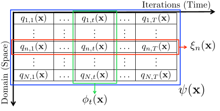
Figure 1: Graphical representation of the $J=NT$ proposal pdfs used in the generalized adaptive multiple IS scheme, spread through the state space $\mathcal{X}$ ($n=1,\ldots,N$) and adapted over time ($t=1,\ldots,T$). Three different mixtures are displayed: $\psi({\bf x})$ involving all the proposals, $\phi_{t}({\bf x})$ involving only the proposals at the $t$-th iteration, and $\xi_{n}({\bf x})$ considering the temporal evolution of the $n$-th proposal pdf.

In an AIS algorithm, one weight

$$w_{n,t}^{(m)}=\frac{\pi({\bf x}_{n,t}^{(m)})}{\Phi_{n,t}({\bf x}_{n,t}^{(m)})},$$ (22)

is associated to each sample ${\bf x}_{n,t}^{(m)}$. In a standard MIS approach, the function employed in the denominator is

$$\Phi_{n,t}({\bf x})=q_{n,t}({\bf x}).$$ (23)

In the complete DM-MIS case, the function $\Phi_{n,t}$ is

$$\Phi_{n,t}({\bf x})=\psi({\bf x})=\frac{1}{NT}\sum_{k=1}^{N}\sum_{r=1}^{T}q_{k,r}({\bf x}).$$ (24)

This case corresponds to the external blue rectangle in Fig. 1. Two natural alternatives of partial DM-MIS schemes appear in this scenario. The first one uses the following partial mixture

$$\Phi_{n,t}({\bf x})=\xi_{n}({\bf x})=\frac{1}{T}\sum_{r=1}^{T}q_{n,r}({\bf x}),$$ (25)

with $n=1,\ldots,N$, in the denominator of the IS weight. Namely, we consider the temporal evolution of the $n$-th single proposal $q_{n,t}$. Hence, we have $L=N$ mixtures, each one formed by $P=T$ components (horizontal red rectangle in Fig. 1). The other possibility is considering the mixture of all the $q_{n,t}$’s at the $t$-th iteration, i.e.,

$$\Phi_{n,t}({\bf x})=\phi_{t}({\bf x})=\frac{1}{N}\sum_{k=1}^{N}q_{k,t}({\bf x}),$$ (26)

for $t=1,\ldots,T$, so that we have $L=T$ mixtures, each one formed by $P=N$ components (vertical green rectangle in Fig. 1). The function $\Phi_{n,t}$ in Eq. (23) is used in the standard PMC scheme (Cappe04, ); Eq. (25) with $N=1$ has been considered in adaptive multiple importance sampling (AMIS) (CORNUET12, ). Eq. (26) has been applied in the adaptive population importance sampling (APIS) algorithm (APIS15, ), whereas in other techniques, such as Mixture PMC (pmc-cappe08, ; Douc07a, ; Douc07b, ), a similar strategy is employed but using a standard sampling of the mixture $\phi_{t}({\bf x})$.

Table 3: Summary of possible MIS strategies in an adaptive framework.

MIS approach	Function $\Phi_{n,t}({\bf x})$	${\bf J}$	${\bf L}$	${\bf P}$	Corresponding Algorithm
			$LP=J$
Standard MIS	$q_{n,t}({\bf x})$		$NT$	$1$	PMC (Cappe04, )
DM-MIS	$\psi({\bf x})=\frac{1}{NT}\sum_{n=1}^{N}\sum_{t=1}^{T}q_{n,t}({\bf x})$		$1$	$NT$	suggested in (LetterVictor, )
Partial DM-MIS	$\xi_{n}({\bf x})=\frac{1}{T}\sum_{t=1}^{T}q_{n,t}({\bf x})$	$NT$	$N$	$T$	AMIS (CORNUET12, ), with $N=1$
Partial DM-MIS	$\phi_{t}({\bf x})=\frac{1}{N}\sum_{n=1}^{N}q_{n,t}({\bf x})$		$T$	$N$	APIS (APIS15, ) and (pmc-cappe08, ; Douc07a, ; Douc07b, )
Partial DM-MIS	generic $\Phi_{n,t}({\bf x})$ in Eq. (27)		$L$	$P$	suggested in (LetterVictor, )

Table 3 summarizes all the possible cases discussed above. The last row corresponds to a generic grouping strategy of the proposal pdfs $q_{n,t}$. As previously described, we can also divide the $J=NT$ proposals into $L=\frac{NT}{P}$ disjoint groups forming $L$ mixtures with $P$ components. We denote the set of $P$ pairs of indices corresponding to the $\ell$-th mixture ($\ell=1,\ldots,L$) as $\mathcal{S}_{\ell}=\{(k_{\ell,1},r_{\ell,1}),\dots,(k_{\ell,P},r_{\ell,P})\}$, where $k_{\ell,p}\in\{1,\ldots,N\}$, $r_{\ell,p}\in\{1,\ldots,T\}$ (i.e., $|\mathcal{S}_{\ell}|=P$, with each element being a pair of indices), and $\mathcal{S}_{r}\cap\mathcal{S}_{\ell}=\emptyset$ for all $\ell=1,\ldots,L,$ and $r\neq\ell$. In this scenario, we have

$$\Phi_{n,t}({\bf x})=\frac{1}{P}\sum_{(k,r)\in\mathcal{S}_{\ell}}q_{k,r}({\bf x}),\quad\mbox{with}\quad(n,t)\in\mathcal{S}_{\ell}.$$ (27)

Note that, using $\psi({\bf x})$ and $\xi_{n}({\bf x})$, the computational cost per iteration increases as the total number of iterations $T$ grows. Indeed, at the $t$-th iteration all the previous proposals $q_{n,1},\ldots,q_{n,t-1}$ (for all $n$) must be evaluated at all the new samples ${\bf x}_{n,t}^{(m)}$. Hence, algorithms based on these proposals quickly become unfeasible as the number of iterations grows. On the other hand, using $\phi_{t}({\bf x})$ the computational cost per iteration is controlled by $N$, remaining invariant regardless of the number of adaptive steps performed.

Observe also that a suitable AIS scheme builds iteratively a global IS estimator which uses the normalized weights

$$\bar{\rho}_{n,t}^{(m)}=\frac{w_{n,t}^{(m)}}{\sum_{\tau=1}^{T}\sum_{n=1}^{N}\sum_{m=1}^{M}w_{n,\tau}^{(m)}},$$ (28)

for $n=1,\ldots,N$, $m=1,\ldots,M$, and $t=1,\ldots,T$.

Table 4 shows an iterative version of GAMIS. We remark that, at the $t$-th iteration, the weights of the samples previously generated need to be recalculated, as shown in step 2(c-3) of Table 4. The choices $\Phi_{n,t}({\bf x})=q_{n,t}({\bf x})$ or $\Phi_{n,t}({\bf x})=\phi_{t}({\bf x})$ allow avoiding completely this re-computation step of the weights. For simplicity, in Table 4 we have provided the output of the algorithms as weighted samples, i.e., all the pairs $\{{\bf x}_{n,t}^{(m)},\bar{\rho}_{n,t}^{(m)}\}$. However, the output can be equivalently expressed as an estimator of a specific moment of the target. In this case, the final IS estimators $\hat{I}_{T}$ and $\hat{Z}_{T}$ are

$$\begin{split}{\hat{I}}_{T}&=\sum_{\tau=1}^{T}\sum_{n=1}^{N}\sum_{m=1}^{M}\bar{\rho}_{n,\tau}^{(m)}f({\bf x}_{n,\tau}^{(m)}),\\ {\hat{Z}}_{T}&=\frac{1}{NMT}\sum_{\tau=1}^{T}\sum_{n=1}^{N}\sum_{m=1}^{M}w_{n,\tau}^{(m)},\end{split}$$ (29)

where $\bar{\rho}_{n,\tau}^{(m)}=\frac{w_{n,\tau}^{(m)}}{{NMT\hat{Z}}_{T}}$. Moreover, the final particle approximation is

$$\hat{\pi}^{(NMT)}({\bf x})=\frac{1}{NMT\hat{Z}_{T}}\sum_{\tau=1}^{T}\sum_{n=1}^{N}\sum_{m=1}^{M}w_{n,\tau}^{(m)}\delta({\bf x}-{\bf x}_{n,\tau}^{(m)}).$$ (30)

The estimators in Eq. (29) can be expressed recursively, thus providing an estimate at each iteration $t$, as stated before. Starting with $H_{0}=0$, ${\hat{I}}_{0}=0$, and setting $S_{t}=\sum_{n=1}^{N}\sum_{m=1}^{M}w_{n,t}^{(m)}$ and $H_{t}=H_{t-1}+S_{t}$, we have

$${\hat{I}}_{t} = \frac{1}{H_{t}}\left[H_{t-1}{\hat{I}}_{t-1}+\sum_{n=1}^{N}\sum_{m=1}^{M}w_{n,t}^{(m)}f({\bf x}_{n,t}^{(m)})\right],$$ (31)

$$= \frac{H_{t-1}}{H_{t-1}+S_{t}}{\hat{I}}_{t-1}+\frac{S_{t}}{H_{t-1}+S_{t}}{\hat{A}}_{t},$$

where ${\hat{A}}_{t}=\sum_{n=1}^{N}\sum_{m=1}^{M}\frac{w_{n,t}^{(m)}}{S_{t}}f({\bf x}_{n,t}^{(m)})$ is the partial IS estimator using only the samples drawn at the $t$-th iteration. Therefore, ${\hat{I}}_{t}$ can be seen as a convex combination of the two IS estimators ${\hat{I}}_{t-1}$ and ${\hat{A}}_{t}$ (for further explanations see Eqs. (46)-(47) in Appendix B.3). Finally, note that

$${\hat{Z}}_{t}=\frac{1}{t}\frac{1}{NM}H_{t}.$$ (32)

A brief discussion about the consistency of ${\hat{I}}_{t}$ and ${\hat{Z}}_{t}$ is provided in Appendix A.

Table 4: GAMIS scheme: iterative version.

1. Initialization: Set $t=1$, $H_{0}=0$ and choose $N$ initial proposal pdfs $q_{n,0}({\bf x})$. 2. For $t=1,\ldots,T$: (a) Adaptation: update the proposal pdfs $\{q_{n,t-1}\}_{n=1}^{N}$ providing $\{q_{n,t}\}_{n=1}^{N}$, using a preestablished procedure (e.g., see (Cappe04, ; pmc-cappe08, ; CORNUET12, ; APIS15, ) for some specific approaches). (b) Generation: Draw $M$ samples from each $q_{n,t}$, i.e., ${\bf x}_{n,t}^{(m)}\sim q_{n,t}({\bf x})$, with $n=1,\ldots,N$ and $m=1,\ldots,M$. (c) Weighting: (c-1) Update the function $\Phi_{n,t}({\bf x})$ given the current population $\{q_{1,t},\ldots,q_{N,t}\}$. (c-2) Assign the weights to the new samples ${\bf x}_{n,t}^{(m)}$, $$w_{n,t}^{(m)}=\frac{\pi({\bf x}_{n,t}^{(m)})}{\Phi_{n,t}({\bf x}_{n,t}^{(m)})},$$ (33) for $n=1,\ldots,N$, and $m=1,\ldots,M$. (c-3) Re-weight the previous samples ${\bf x}_{n,\tau}^{(m)}$ for $\tau=1,\ldots,t-1$ as $$w_{n,\tau}^{(m)}=\frac{\pi({\bf x}_{n,\tau}^{(m)})}{\Phi_{n,t}({\bf x}_{n,\tau}^{(m)})},$$ (34) with $\tau=1,\ldots,t-1$, $n=1,\ldots,N$, and $m=1,\ldots,M$. (d) Normalization: Set $S_{t}=\sum_{m=1}^{M}\sum_{n=1}^{N}w_{n,t}^{(m)}$, $H_{t}=H_{t-1}+S_{t}$ , and re-normalize all the weights, $$\bar{\rho}_{n,\tau}^{(m)}=\bar{\rho}_{n,\tau-1}^{(m)}\frac{H_{t-1}}{H_{t}},$$ (35) for $\tau=1,\ldots,t$, $n=1,\ldots,N$, and $m=1,\ldots,M$. (e) Output: Return all the pairs $\{{\bf x}_{n,\tau}^{(m)},\bar{\rho}_{n,\tau}^{(m)}\}$, for $\tau=1,\ldots,t$, $n=1,\ldots,N$, and $m=1,\ldots,M$.

5 Markov adaptation for GAMIS

In this section, we design efficient adaptive importance sampling (AIS) techniques by combining the main ideas discussed in the two previous sections. More specifically, we apply the hierarchical MC approach to adapt the proposal pdfs within a GAMIS scheme. Therefore, a Markov GAMIS technique, or simply Markov Adaptive Importance Sampling (MAIS) algorithm, consists of the following two layers:

• Upper level (Adaptation): Given the set of mean vectors,

  $$\mathcal{P}_{t-1}=\{{\bm{\mu}}_{1,t-1},\ldots,{\bm{\mu}}_{N,t-1}\},$$

  obtain the new set $\mathcal{P}_{t}=\{{\bm{\mu}}_{1,t},\ldots,{\bm{\mu}}_{N,t}\}$ according to MCMC transitions with $\bar{\pi}$ as invariant density. More specifically, a kernel $K({\bm{\mu}}_{1:N,t}|{\bm{\mu}}_{1:N,t-1})$ leaving invariant the distribution $\prod_{n=1}^{N}{\bar{\pi}}({\bm{\mu}}_{n})$ is applied.

• Lower level (MIS estimator): Given the population of proposals,

  $$q_{1,t}({\bf x}|{\bm{\mu}}_{1,t},{\bf C}_{1}),\ldots,q_{N,t}({\bf x}|{\bm{\mu}}_{N,t},{\bf C}_{N}),$$

  choose a function $\Phi_{n,t}({\bf x})$ for the computation of the weights in Eq. (22), and perform a MIS approximation of the target as described in Section 4.2.

5.1 Theoretical support: adaptation and consistency

The motivation behind the MCMC adaptation has been described in Section 3.2 and 3.3: the functions $q_{n,t}$, located at the ${\bm{\mu}}_{n,t}$’s, jointly provide a kernel estimate of the target ${\bar{\pi}}$.

Furthermore, we recall that the generation of the means, ${\bm{\mu}}_{n,t}$, is completely independent from the samples ${\bf x}_{n,t}$ drawn in the lower level. This is a key point from a theoretical and practical point of view. Indeed, the generic MAIS algorithm can be divided in two steps: (a) first generate all the means $\{{\bm{\mu}}_{n,t}\}_{t=1}^{T}$ for $n=1,\ldots,N$, (b) then perform the MIS estimation considering all the proposals $q_{n,t}({\bf x}|{\bm{\mu}}_{n,t},{\bf C}_{n})$, $\forall n$ and $\forall t$. Namely, any MAIS technique can be converted into a generalized static MIS scheme (see Section 4.1). As a consequence, the unique conditions required for ensuring the consistency of the corresponding estimators are ElviraMIS15 ; Robert04 :

• All the proposal pdfs, $q_{n,t}$, must have heavier tails than the target ${\bar{\pi}}$.

• A suitable function $\Phi_{n,t}({\bf x})$ for the denominator of the importance weights must be chosen. Namely, the use of $\Phi_{n,t}({\bf x})$ provides consistent estimators ElviraMIS15 , like the functions $\Phi_{n,t}({\bf x})$ described in Section 4.2.

Moreover, the independence of the upper level from the lower level of the hierarchical approach, helps the parallelization of the algorithms as we discuss later.

Table 5 compares different AIS schemes. In the standard AIS method Bugallo15 , the sequence of $\{{\bm{\mu}}_{n,t}\}$ converges to a unknown fixed vector as $t\rightarrow\infty$. In the standard PMC algorithm Cappe04 , the limiting distribution of $\{{\bm{\mu}}_{n,t}\}$ is unknown. Furthermore, in both cases, standard AIS and PMC, the adaptation depends on the previously generated samples ${\bf x}$’s. In MAIS techniques, the use of an ergodic chain (with invariant pdf ${\bar{\pi}}$) for generating the $n$-th mean vector ${\bm{\mu}}_{n,t}$ ensures that its asymptotic density is ${\bar{\pi}}({\bm{\mu}})$.

Table 5: Adaptation of the mean vectors $\{{\bm{\mu}}_{n,t}\}$ using different AIS techniques.

Features	Stand. AIS	PMC	MAIS
limiting	(unknown)	unknown
distribution of	fixed	(if/when	${\bar{\pi}}({\bm{\mu}})$
$\{{\bm{\mu}}_{n,t}\}$ for $t\rightarrow\infty$	vector	exists)
dependence of
the adaptation	yes	yes	no
w.r.t. the ${\bf x}$’s

5.2 The new class of algorithms

Markov GAMIS framework can lead to many different algorithms, depending on the MCMC strategy used to update the mean vectors and the specific choice of the function $\Phi_{n,t}$. Table 6 provides several examples of novel techniques determined by the value of $N$, the choice of $\Phi_{n,t}$, and the type of MCMC adaptation. Some of them are variants of well-known techniques like PMC (Cappe04, ) and AMIS (CORNUET12, ), where the Markov adaptation procedure is employed. Others, such as the Random Walk Importance Sampling (RWIS), the Parallel Interacting Markov Adaptive Importance Sampling (PI-MAIS) and Doubly Interacting Markov Adaptive Importance Sampling (I²-MAIS), are described below in detail. For these completely novel algorithms we have set $\Phi_{n,t}({\bf x})=\phi_{t}({\bf x})$, so that the computational cost is directly controlled by $N$ and the re-weighting step 2(c-3) in Table 4 is not required.

RWIS is the simplest possible Markov GAMIS algorithm. Specifically, for the MCMC adaptation we consider a standard MH technique, setting $N=1$ and choosing $\Phi_{n,t}({\bf x})=\phi_{t}({\bf x})=q_{n,t}({\bf x})$ (since $N=1$, the two cases coincide). Table 7 shows the RWIS algorithm, which is a special case of the more general scheme described in Table 8 when $N=1$. Note that we have a proposal pdf used for the MH adaptation, $\varphi({\bm{\mu}}|{\bm{\mu}}_{t-1},{\bf\Lambda})$, which is different from the proposal pdf used for the IS estimation, $q({\bf x}|{\bm{\mu}}_{t},{\bf C})$.

Table 6: Example of possible Markov GAMIS algorithms.

		Parallel adaptation	Interacting adaptation
Function $\bm{\Phi}_{n,t}({\bf x})$	${\bf N=1}$	${\bf N>1}$	${\bf N>1}$
$q_{n,t}({\bf x})$				RWIS	Markov PMC (related to (Cappe04, ))
	(see Table 7)
$\xi_{n}({\bf x})=\frac{1}{T}\sum_{t=1}^{T}q_{n,t}({\bf x})$	Markov AMIS	$N$ parallel	Population-based
	(related to (CORNUET12, ))	Markov AMIS (rel. to (CORNUET12, ))	Markov AMIS (rel. to (CORNUET12, ))
$\phi_{t}({\bf x})=\frac{1}{N}\sum_{n=1}^{N}q_{n,t}({\bf x})$	RWIS	PI-MAIS	I2-MAIS
	(see Table 7)	(see Section 5.3)	(see Section 5.3)
$\psi({\bf x})=\frac{1}{NT}\sum_{n=1}^{N}\sum_{t=1}^{T}q_{n,t}({\bf x})$	Markov AMIS	Full Markov GAMIS
	(related to (CORNUET12, ))
generic $\Phi_{n,t}({\bf x})$	Partial Markov GAMIS

Table 7: Random Walk Importance Sampling (RWIS) algorithm.

1. Initialization: start with $t=1$, $H_{0}=0$, choose the values $M$ and $T$, the initial location parameter ${\bm{\mu}}_{0}$, the scale parameters ${\bf C}$ and ${\bm{\Lambda}}$. 2. For $t=1,\ldots,T$: (a) MH step: (a-1) Draw ${\bm{\mu}}^{\prime}\sim\varphi({\bm{\mu}}|{\bm{\mu}}_{t-1},{\bm{\Lambda}})$. (a-2) Set ${\bm{\mu}}_{t}={\bm{\mu}}^{\prime}$ with probability α= min[1,π(μ’)φ(μt—μ’,Λ),π(μt)φ(μ’—μt-1,Λ)], otherwise set ${\bm{\mu}}_{t}={\bm{\mu}}_{t-1}$ (with probability $1-\alpha$). (b) IS steps: (b-1) Draw ${\bf x}_{t}^{(m)}\sim q_{t}({\bf x}|{\bm{\mu}}_{t},{\bf C}_{n})$ for $m=1,\ldots,M$. (b-2) Weight the samples as w_t^(m)=π(xt(m))qt(xt(m)—μt,Cn). (b-3) Set $S_{t}=\sum_{m=1}^{M}w_{t}^{(m)}$, $H_{t}=H_{t-1}+S_{t}$, and normalize the weights ¯ρ_t^(m)= wt(m)∑τ=1t∑r=1Mwτ(r)=¯ρ_t-1^(m) Ht-1Ht. (c) Output: Return all the pairs $\{{\bf x}_{\tau}^{(m)},\bar{\rho}_{\tau}^{(m)}\}$ for $m=1,\ldots,M$ and $\tau=1,\ldots,t$.

5.3 Population-based algorithms

The RWIS technique can be easily extended by using a population of $N$ proposal pdfs. In this case, we choose

$$\Phi_{n,t}({\bf x})=\phi_{t}({\bf x})=\frac{1}{N}\sum_{n=1}^{N}q_{n,t}({\bf x}),$$

so that the computational cost of evaluating the mixture $\Phi_{n,t}({\bf x})=\phi_{t}({\bf x})$ depends only on $N$, regardless of the number $t$ of iterations. Moreover, step 2(c-3) in Table 4 is not required in this case. Table 8 describes the corresponding algorithm without specifying the MCMC approach used for generating the population of means, ${\bf\mathcal{P}}_{t}=\{{\bm{\mu}}_{1,t},...,{\bm{\mu}}_{N,t}\}$, given ${\bf\mathcal{P}}_{t-1}$.

Two possible adaptation procedures via MCMC are discussed below. In the first one, we consider $N$ independent parallel chains for updating the $N$ mean vectors. We refer to this method as Parallel Interacting Markov Adaptive Importance Sampling (PI-MAIS). Although PI-MAIS is parallelizable, in the iterative version of Table 8 the $N$ independent processes cooperate together in Eq. (36) to provide unique global IS estimate. In the second adaptation scheme, we introduce the interaction also in the upper level. Hence, we refer to this method as Doubly Interacting Markov Adaptive Importance Sampling (I²-MAIS). In both cases, the corresponding technique provides an IS approximation of the target or, equivalently, the estimators $\hat{I}_{T}$ and $\hat{Z}_{T}$ in Eq. (29), using $NMT$ samples.

Table 8: Population-Based MAIS algorithms.

1. Initialization: Set $t=1$, $\hat{I}_{0}=0$ and $H_{0}=0$. Choose the initial population P_0={μ_1,0,…,μ_N,0}, and $N$ covariance matrices ${\bf C}_{n}$ ($n=1,\ldots,N$). Choose also the parametric form of the $N$ normalized proposals $q_{i,t}$ with parameters ${\bm{\mu}}_{n,t}$ and ${\bf C}_{n}$. Let $T$ be the total number of iterations. 2. For $t=1,\ldots,T$: (a) Update of the location parameters: Perform one transition of one or more MCMC techniques over the current population, P_t-1={μ_1,t-1,…,μ_N,t-1}, obtaining a new population, P_t={μ_1,t,…,μ_N,t}. (b) IS steps: (b-1) Draw ${\bf x}_{n,t}^{(m)}\sim q_{n,t}({\bf x}|{\bm{\mu}}_{n,t},{\bf C}_{n})$ for $m=1,\ldots,M$ and $n=1,\ldots,N$. (b-2) Compute the importance weights, $$w_{n,t}^{(m)}=\frac{\pi({\bf x}_{n,t}^{(m)})}{\frac{1}{N}\sum_{k=1}^{N}q_{k,t}({\bf x}_{n,t}^{(m)}|{\bm{\mu}}_{k,t},{\bf C}_{k})},$$ (36) with $n=1,\ldots,N$, and $m=1,\ldots,M$. (b-3) Set $S_{t}=\sum_{n=1}^{N}\sum_{m=1}^{M}w_{n,t}^{(m)}$, $H_{t}=H_{t-1}+S_{t}$, and normalize the weights $\displaystyle\bar{\rho}_{n,t}^{(m)}$ $\displaystyle=$ $\displaystyle\frac{w_{n,t}^{(m)}}{\sum_{\tau=1}^{t}\sum_{i=1}^{N}\sum_{r=1}^{M}w_{i,\tau}^{(r)}}$ $\displaystyle=$ $\displaystyle\bar{\rho}_{n,t-1}^{(m)}\frac{H_{t-1}}{H_{t}}.$ (c) Outputs: Return all the pairs $\{{\bf x}_{\tau}^{(m)},\bar{\rho}_{\tau}^{(m)}\}$ for $m=1,\ldots,M$ and $\tau=1,\ldots,t$.

5.3.1 MCMC adaptation for PI-MAIS

The simplest option is applying one iteration of $N$ parallel MCMC chains, one for each ${\bm{\mu}}_{n,t-1}$ returning ${\bm{\mu}}_{n,t}$, for $n=1,\ldots,N$. For instance, given $N$ parallel MH transitions, each one employing (possibly) a different proposal pdf $\varphi_{n}$ with covariance matrix ${\bf\Lambda}_{n}$, we have:

For $n=1,\ldots,N$:

1. Draw ${\bm{\mu}}^{\prime}\sim\varphi_{n}({\bm{\mu}}|{\bm{\mu}}_{n,t-1},{\bf\Lambda}_{n})$.

2. Set ${\bm{\mu}}_{n,t}={\bm{\mu}}^{\prime}$ with probability

   $$\alpha=\min\left[1,\frac{\pi({\bm{\mu}}^{\prime})\varphi_{n}({\bm{\mu}}_{n,t-1}|{\bm{\mu}}^{\prime},{\bf\Lambda}_{n})}{\pi({\bm{\mu}}_{n,t-1})\varphi_{n}({\bm{\mu}}^{\prime}|{\bm{\mu}}_{n,t-1},{\bf\Lambda}_{n})}\right],$$

   otherwise set ${\bm{\mu}}_{n,t}={\bm{\mu}}_{n,t-1}$ (with probability $1-\alpha$).

Figure 2(a) illustrates this scenario. Each mean vector ${\bm{\mu}}_{n,t}$ is updated independently from the rest. Therefore, in PI-MAIS, the interaction among the different processes occurs only in the underlying IS layer of the hierarchical structure: the importance weights in Eq. (36) are built using the partial DM-MIS strategy with $\phi_{t}({\bf x})=\frac{1}{N}\sum_{n=1}^{N}q_{n,t}({\bf x}|{\bm{\mu}}_{n,t},{\bf C}_{n})$. Considerations about the parallelization of PI-MAIS are given in Section 5.5.

           

(a) For PI-MAIS

(b) For I²-MAIS

(c) For I²-MAIS

(d) For I²-MAIS

Figure 2: Different possible adaptation procedures for Population-based MAIS schemes. (a) One transition of $N$ independent parallel MH chains (${\bm{\mu}}_{n,t}\in\mathbb{R}^{D_{x}}$) for PI-MAIS. (b) One transition of an MH method working in the extended space $[{\bm{\mu}}_{1,t},\ldots,{\bm{\mu}}_{N,t}]\in\mathbb{R}^{D_{x}\times N}$. (c) One transition of SMH (Liang10, , Chapter 5), considering the population of mean vectors $\mathcal{P}_{t}=\{{\bm{\mu}}_{1,t},...,{\bm{\mu}}_{N,t}\}$. (d) $N$ sequential transitions of (possibly) different MH kernels starting from ${\bm{\mu}}_{0,t}={\bm{\mu}}_{N,t-1}$.

5.3.2 MCMC adaptation for I²-MAIS

Let us consider an extended state space $\mathbb{R}^{D_{x}\times N}$ and an extended target pdf

$$\bar{\pi}_{g}({\bm{\mu}}_{1},\ldots,{\bm{\mu}}_{N})\propto\prod_{n=1}^{N}\pi({\bm{\mu}}_{n}),$$ (37)

where each marginal $\pi({\bm{\mu}}_{n})$, for $i=1,...,N$, coincides with the target in Eq. (2). In this section, we describe three interacting adaptation procedures for the mean vectors, which consider the generalized pdf in Eq. (37) as invariant density. They are represented graphically in Figs. 2(b), (c) and (d).

MH in the extended space $\mathbb{R}^{D_{x}\times N}$

The simplest possibility is applying directly a block-MCMC technique, transitioning from the matrix

$${\bf P}_{t-1}=[{\bm{\mu}}_{1,t-1},\ldots,{\bm{\mu}}_{N,t-1}],$$

to the matrix ${\bf P}_{t}=[{\bm{\mu}}_{1,t},\ldots,{\bm{\mu}}_{N,t}]$. Let us consider an MH method and a proposal pdf $\varphi({\bf P}_{t}|{\bf P}_{t-1}):\mathbb{R}^{D_{x}\times N}\rightarrow\mathbb{R}^{D_{x}\times N}$. For instance, one can consider a proposal of the type

$$\begin{split}\varphi({\bm{\mu}}_{1,t},\ldots,{\bm{\mu}}_{N,t}|{\bm{\mu}}_{1,t-1},\ldots,&{\bm{\mu}}_{N,t-1})\\ &=\prod_{n=1}^{N}\varphi_{n}({\bm{\mu}}_{n,t}|{\bm{\mu}}_{n,t-1},{\bf\Lambda}_{n}).\end{split}$$

Thus, one transition is formed by the following steps:

1. Draw ${\bf P}^{\prime}\sim\varphi({\bf P}|{\bf P}_{t-1})$, where ${\bf P}^{\prime}=[{\bm{\mu}}_{1}^{\prime},\ldots,{\bm{\mu}}_{N}^{\prime}]$.

2. Set ${\bf P}_{t}={\bf P}^{\prime}$ with probability

   $$\alpha=\min\left[1,\frac{\pi_{g}({\bf P}^{\prime})\varphi({\bf P}_{t-1}|{\bf P}^{\prime})}{\pi_{g}({\bf P}_{t-1})\varphi({\bf P}^{\prime}|{\bf P}_{t-1})}\right],$$

   otherwise set ${\bf P}_{t}={\bf P}_{t-1}$ (with probability $1-\alpha$).

At each iteration, $N$ new samples ${\bm{\mu}}_{n}^{\prime}$ are drawn (as in PI-MAIS) and therefore $N$ new evaluations of $\pi$ are required (i.e., one evaluation of $\pi_{g}$). When a new ${\bf P}^{\prime}$ is accepted, all the components of ${\bf P}_{t}$ differ from ${\bf P}_{t-1}$, unlike in the strategy described later. However, the probability of accepting a new population becomes very small for large values of $N$.

Sample Metropolis-Hastings (SMH) algorithm

SMH is a population-based MCMC technique, suitable for our purposes (Liang10, , Chapter 5). At each iteration $t$, given the previous set

$${\bf\mathcal{P}}_{t-1}=\{{\bm{\mu}}_{1,t-1},...,{\bm{\mu}}_{N,t-1}\},$$

a new possible parameter ${\bm{\mu}}_{0,t-1}$, drawn from an independent proposal $\varphi({\bm{\mu}})$, is tested to be interchanged with another parameter in ${\bf\mathcal{P}}_{t-1}=\{{\bm{\mu}}_{1,t-1},...,{\bm{\mu}}_{N,t-1}\}$. The underlying idea of SMH is to replace one “bad” sample in the population ${\bf\mathcal{P}}_{t-1}$ with a potentially “better” one, according to a certain suitable probability $\alpha$. The algorithm is designed so that, after a burn-in period, the elements in ${\bf\mathcal{P}}_{t}$ are distributed according to ${\bar{\pi}}_{g}({\bm{\mu}}_{1},\ldots,{\bm{\mu}}_{N})$. One iteration of SMH consists of the following steps:

1. Draw a candidate ${\bm{\mu}}_{0,t-1}\sim\varphi({\bm{\mu}})$.

2. Choose a “bad” sample, ${\bm{\mu}}_{k,t-1}$ with $k\in\{1,...,N\}$, from the population according to a probability proportional to $\frac{\varphi({\bm{\mu}}_{k,t-1})}{\pi({\bm{\mu}}_{k,t-1})}$, which corresponds to the inverse of the standard IS weights.

3. Accept the new population, $\mathcal{P}_{t}=\{{\bm{\mu}}_{1,t},\ldots,{\bm{\mu}}_{N,t}\}$ with ${\bm{\mu}}_{n,t}={\bm{\mu}}_{n,t-1}$ for all $n\neq k$ and ${\bm{\mu}}_{k,t}={\bm{\mu}}_{0,t-1}$, with probability

   $$\alpha(\mathcal{P}_{t-1},{\bm{\mu}}_{0,t-1})=\frac{\sum_{n=1}^{N}\frac{\varphi({\bm{\mu}}_{n,t-1})}{\pi({\bm{\mu}}_{n,t-1})}}{\sum_{i=0}^{N}\frac{\varphi({\bm{\mu}}_{i,t-1})}{\pi({\bm{\mu}}_{i,t-1})}-\min\limits_{0\leq i\leq N}\frac{\varphi({\bm{\mu}}_{i,t-1})}{\pi({\bm{\mu}}_{i,t-1})}}.$$

   Otherwise, set ${\bf\mathcal{P}}_{t}={\bf\mathcal{P}}_{t-1}$.

Unlike in the previous strategy, the difference between ${\bf\mathcal{P}}_{t-1}$ and ${\bf\mathcal{P}}_{t}$ is at most one sample. Observe that $\alpha$ depends on $\mathcal{P}_{t-1}$ and the candidate ${\bm{\mu}}_{0,t-1}$. However, at each iteration, only one new evaluation of $\pi$ (and $\varphi$) is needed at ${\bm{\mu}}_{0,t-1}$, since the rest of the weights have already been computed in the previous steps (except for the initial iteration).

MH within Gibbs

Another simple alternative, following an “MH within Gibbs” approach for sampling from ${\bar{\pi}}_{g}$, is to update sequentially each ${\bm{\mu}}_{n,t-1}$ using one MH step in $\mathbb{R}^{D_{x}}$. Hence, setting ${\bm{\mu}}_{0,t}={\bm{\mu}}_{N,t-1}$, we have:

For $n=1,\ldots,N$:

1. Draw ${\bm{\mu}}^{\prime}$ from a proposal pdf $\varphi_{n}({\bm{\mu}}|{\bm{\mu}}_{n-1,t},{\bf\Lambda}_{n})$.

2. Set ${\bm{\mu}}_{n,t}={\bm{\mu}}^{\prime}$ with probability

   $$\alpha=\min\left[1,\frac{\pi({\bm{\mu}}^{\prime})\varphi_{n}({\bm{\mu}}_{n-1,t}|{\bm{\mu}}^{\prime},{\bf\Lambda}_{n})}{\pi({\bm{\mu}}_{n-1,t})\varphi_{n}({\bm{\mu}}^{\prime}|{\bm{\mu}}_{n-1,t},{\bf\Lambda}_{n})}\right],$$

   otherwise set ${\bm{\mu}}_{n,t}={\bm{\mu}}_{n-1,t}$.

This scenario is illustrated in Fig. 2(d). In this case, after $T$iterations of the I²-MAIS scheme, we generate a unique MH chain with $NT$ total states, divided in $T$ parts of $N$ states. At each iteration of the I²-MAIS scheme, each block of $N$ states is employed as mean vector of the $N$ proposal pdfs used in the lower level.

5.4 Computational cost: comparison between PI-MAIS and I²-MAIS

In all cases, the total number of samples involved in the final estimation is $NMT$. The total number of evaluations of the target, $E$, is larger due to the MCMC implementation, i.e., $E>NMT$. More precisely, the total number of evaluations of the target is:

• $E=MNT+NT$, for PI-MAIS,

• $E=MNT+NT$, for I²-MAIS with MH in the extended space $\mathbb{R}^{D_{X}\times N}$,

• $E=MNT+T$, for I²-MAIS with SMH,

• $E=MNT+NT$, for I²-MAIS with the MH-within-Gibbs approach.

Note that we have taken into account that several evaluations of the target have been computed in the previous iterations. Moreover, the application of the MCMC techniques requires generation of $V$ additional uniform r.v.’s for performing the acceptance tests (and additional r.v.’s for choosing a “bad” candidate in SMH). Specifically, we need: $V=NT$ uniform r.v.’s in PI-MAIS and I²-MAIS with MH-within-Gibbs, $V=T$ uniform r.v.’s for I²-MAIS with MH in the extended space, and$V=2T$, $T$ uniform r.v. and $T$ multinomial r.v., for I²-MAIS with SMH. However, in practical applications, the main computational effort is usually required for the target evaluation. The computing time required in the multinomial sampling within SMH increases with $N$. Finally, we recall that we have used a deterministic mixture weighting scheme with $\Phi_{n,t}({\bf x})=\phi_{t}({\bf x})$, which requires $MN^{2}T$ evaluations of the proposal pdfs, $q_{n,t}({\bf x})$, for $n=1,\ldots,N$ and $t=1,\ldots,T$.

5.5 Non-iterative and parallel implementations

As remarked in Section 5.1, the choice of the means ${\bm{\mu}}_{n,t}$’s is completely independent from the estimation steps. Thus, all the means can be selected in advance (also in parallel if the strategy in Section 5.3.1 is used), and the MIS estimation steps can then be performed as in a completely static framework (i.e., as described in Section 4.1). This consideration is valid for any choice of $\Phi_{n,t}({\bf x})$.

Let us consider now the choice of $\Phi_{n,t}$’s as temporal mixtures, i.e., $\Phi_{n,t}=\frac{1}{T}\sum_{t=1}^{T}q_{n,t}({\bf x})$ or $\Phi_{n,t}({\bf x})=q_{n,t}({\bf x})$. Moreover, let us consider the use of $N$ parallel MCMC chains for adapting the means, i.e., one independent chain for each parameter ${\bm{\mu}}_{n,t}$, with $n=1,\ldots,N$. In this case, the corresponding algorithm is completely parallelizable. Indeed, it can be decomposed into $N$ parallel MAIS techniques, each one producing the partial estimators ${\hat{I}}_{n,T}$ and ${\hat{Z}}_{n,T}$, after $T$ iterations. The global estimators are then given by

$$\begin{split}{\hat{I}}_{T}&=\sum_{n=1}^{N}\frac{{\hat{Z}}_{n,T}}{\sum_{i=1}^{N}{\hat{Z}}_{i,T}}{\hat{I}}_{n,T},\\ {\hat{Z}}_{T}&=\frac{1}{N}\sum_{n=1}^{N}{\hat{Z}}_{n,T}.\end{split}$$ (38)

Furthermore, different strategies for sharing information among the parallel chains can also be applied (Craiu09, ; O-MCMC, ; Smelly, ; Geyer91, ; Marinari92, ; Neal01, ), or for reducing the total number of evaluations of the target Jacob11 (the scheme in Jacob11 can be applied if a unique independent proposal is employed, i.e., $\varphi_{n}({\bm{\mu}})=\varphi({\bm{\mu}})$ for all $n$).

6 Numerical simulations

In this section, we test the performance of the proposed scheme comparing them with other benchmark techniques. First of all, we tackle two challenging issues for adaptive Monte Carlo methods: multimodality in Section 6.1 and nonlinearity in Section 6.2. Furthermore, in Section 6.4 we consider an application of positioning and tuning model parameters in a wireless sensor network (Ali07, ; Ihler05, ; MartinoStatCo10, ).

6.1 Multimodal target distribution

In this section, we test the novel proposed algorithms in a multimodal scenario, comparing with several other methods. Specifically, we consider a bivariate multimodal target pdf, which is itself a mixture of $5$ Gaussians, i.e.,

$$\bar{\pi}({\bf x})=\frac{1}{5}\sum_{i=1}^{5}\mathcal{N}({\bf x};{\bf\nu}_{i},{\bf\Sigma}_{i}),\quad{\bf x}\in\mathbb{R}^{2},$$ (39)

with means ${\bf\nu}_{1}=[-10,-10]^{\top}$, ${\bf\nu}_{2}=[0,16]^{\top}$, ${\bf\nu}_{3}=[13,8]^{\top}$, ${\bf\nu}_{4}=[-9,7]^{\top}$, ${\bf\nu}_{5}=[14,-14]^{\top}$, and covariance matrices ${\bf\Sigma}_{1}=[2,\ 0.6;0.6,\ 1]$, ${\bf\Sigma}_{2}=[2,\ -0.4;-0.4,\ 2]$, ${\bf\Sigma}_{3}=[2,\ 0.8;0.8,\ 2]$, ${\bf\Sigma}_{4}=[3,\ 0;0,\ 0.5]$ and ${\bf\Sigma}_{5}=[2,\ -0.1;-0.1,\ 2]$. The main challenge in this example is the ability in discovering the $5$ different modes of $\bar{\pi}({\bf x})\propto\pi({\bf x})$. Since we know the moments of $\pi({\mathbf{x}})$, we can easily assess the performance of the different techniques.

Given a random variable (r.v.) ${\bf X}\sim{\bar{\pi}}({\bf x})$, we consider the problem of approximating via Monte Carlo the expected value $E[{\bf X}]=[1.6,1.4]^{\top}$ and the normalizing constant $Z=1$. Note that an adequate approximation of $Z$ requires the ability of learning about all the $5$ modes. We compare the performances of different sampling algorithms in terms of Mean Square Error (MSE): (a) the AMIS technique (CORNUET12, ), (b) three different PMC schemes, two of them proposed in (pmc-cappe08, ; Cappe04, ) and one PMC using a partial DM-MIS scheme with $\Phi_{n,t}({\bf x})=\phi_{t}({\bf x})$, (c) $N$ parallel independent MCMC chains and (d) the proposed PI-MAIS method. Moreover, we test two static MIS approaches, the standard MIS and a partial DM-MIS schemes with $\Phi_{n,t}({\bf x})=\phi_{t}({\bf x})$, computing iteratively the final estimator.

For a fair comparison, all the mentioned algorithms have been implemented in such a way that the number of total evaluations of the target is $E=2\cdot 10^{5}$. All the involved proposal densities are Gaussian pdfs. More specifically, in PI-MAIS, we use the following parameters: $N=100$, $M\in\{1,19,99\}$, $T\in\{20,100,1000\}$ in order to fulfill $E=MNT+NT=(M+1)NT=2\cdot 10^{5}$ (see Section 5.4). The proposal densities of the upper level of the hierarchical approach, $\varphi_{n}({\mathbf{x}}|{\bm{\mu}}_{n,t},{\bf\Lambda}_{n})$, are Gaussian pdfs with covariance matrices ${\bf\Lambda}_{n}=\lambda^{2}{\bf I}_{2}$ and $\lambda\in\{5,10,70\}$. The proposal densities used in the lower importance sampling level, $q_{n,t}({\mathbf{x}}|{\bm{\mu}}_{n,t},{\bf C}_{n})$ are Gaussian pdfs with covariance matrices ${\bf C}_{n}=\sigma^{2}{\bf I}_{2}$ and $\sigma\in\{0.5,1,2,5,10,20,70\}$. We also try different non-isotropic diagonal covariance matrices in both levels, i.e, ${\bf\Lambda}_{n}=\textrm{diag}(\lambda_{n,1}^{2},\lambda_{n,2}^{2})$, where $\lambda_{i,j}\sim\mathcal{U}([1,10])$, and ${\bf C}_{n}=\textrm{diag}(\sigma_{n,1}^{2},\sigma_{n,2}^{2})$, where $\sigma_{n,j}\sim\mathcal{U}([1,10])$ for $j\in\{1,2\}$ and $n=1,\ldots N$. We test all these techniques using two different initializations: first, we choose deliberately a “bad” initialization of the initial mean vectors, denoted as In1, in the sense that the initialization region does not contain the modes of $\pi$. Thus, we can test the robustness of the algorithms and their ability to improve the corresponding static approaches. Specifically, the initial mean vectors are selected uniformly within the following square

$${\bm{\mu}}_{n,0}\sim\mathcal{U}([-4,4]\times[-4,4]),$$

for $n=1,\ldots,N$. Different examples of this configuration are shown in Fig. 3 with squares. Secondly, we also consider a better initialization, denoted as In2, where the initialization region contains all the modes. Specifically, the initial mean vectors are selected uniformly within the following square

$${\bm{\mu}}_{n,0}\sim\mathcal{U}([-20,20]\times[-20,20]),$$

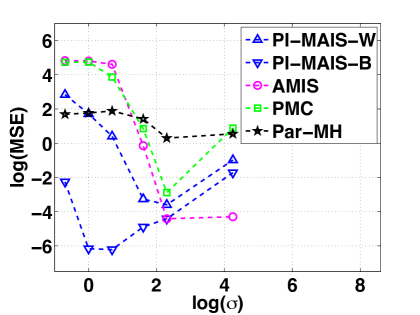
(a) Ex-Sect 6.1

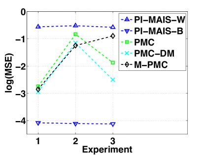
(b) Ex-Sect 6.4

Figure 6: (Ex-Sect 6.1-6.4) Summary of the results in Table 9 in Fig. (a), and Table 13 in Fig. (b): the curve $\log(\mbox{MSE})$ of the different methods as function of $\log(\sigma)$ in Fig. (a) ($\sigma\in\{0.5,1,2,5,10,70\}$), and as function of the different experiments in Fig. (b). The worst and best results of PI-MAIS are depicted with triangles up and down, respectively.

for $n=1,\ldots,N$. All the results are averaged over $2\cdot 10^{3}$ independent experiments. Tables 9 and 10 show the Mean Square Error (MSE) in the estimation of the first component of $E[{\bf X}]$, with the initialization In1 and In2 respectively. Table 11 provides the MSE in the estimation of $Z$ with In1. The best results in each column are highlighted in bold-face. In AMIS (CORNUET12, ), the mean vector and the covariance matrix of a single proposal (i.e., $N=1$) are adapted, using $\Phi_{1,t}({\bf x})=\xi_{1}({\bf x})$ in the computation of the IS weights. Hence, in AMIS, we have tested different values of samples per iterations $M\in\{500,10^{3},2\cdot 10^{3},5\cdot 10^{3},10^{4}\}$ and $T=\frac{E}{M}$. For the sake of simplicity, we directly show the worst and best results among the several simulations made with different parameters. PI-MAIS outperforms the other algorithms virtually for all the choices of the parameters, with both initializations. In general, a greater value of $T$ is needed since the proposal pdfs are initially bad localized. Moreover, PI-MAIS always improves the performance of the static approaches. These two consideration show the benefit of the Markov adaptation. Hence, PI-MAIS presents more robustness with respect to the initial values and the choice of the covariance matrices. Figure 6(a) providing a summary of the results in Table 9 showing the $\log(\mbox{MSE})$ as function of the $\log(\sigma)$, for the main compared methods. Figure 3 depicts the initial (squares) and final (circles) configurations of the mean vectors of the proposal densities for the standard PMC and the PI-MAIS methods, in a specific run and different values of $\sigma,\lambda\in\{3,5\}$. In both cases, PI-MAIS guarantees a better covering of the modes of $\pi({\bf x})$.

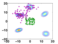
(a) PMC ($N=100$, $\sigma=3$)

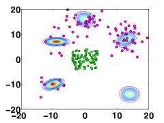
(b) PMC ($N=100$, $\sigma=5$)

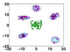
(c) PI-MAIS ($N=100$, $\lambda=3$)

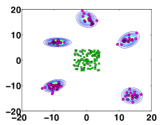
(d) PI-MAIS ($N=100$, $\lambda=5$)

Figure 3: Initial (squares) and final (circles) configurations of the mean vectors of the proposal densities for the standard PMC and the PI-MAIS methods, in different specific runs. The initial configuration corresponds to In1.

6.2 Nonlinear banana-shaped target distribution

Here we consider a bi-dimensional “banana-shaped” target distribution (Haario2001, ), which is a benchmark function in the literature due to its nonlinear nature. Mathematically, it is expressed as

$${\bar{\pi}}(x_{1},x_{2})\propto\exp\left(-\frac{1}{2\eta_{1}^{2}}\left(4-Bx_{1}-x_{2}^{2}\right)^{2}-\frac{x_{1}^{2}}{2\eta_{2}^{2}}-\frac{x_{2}^{2}}{2\eta_{3}^{2}}\right),$$

where, we have set $B=10$, $\eta_{1}=4$, $\eta_{2}=5$, and $\eta_{3}=5$. The goal is to estimate the expected value $E[{X}]$, where ${X}=[X_{1},X_{2}]\sim{\bar{\pi}}(x_{1},x_{2})$, by applying different Monte Carlo approximations. We approximately compute the true value $E[{X}]\approx[-0.4845,0]^{\top}$ using an exhaustive deterministic numerical method (with an extremely thin grid), in order to obtain the mean square error (MSE) of the following methods: standard PMC (Cappe04, ), the Mixture PMC (pmc-cappe08, ), the AMIS (CORNUET12, ), PI-MAIS and I²-MAIS with SMH adaptation.

We consider Gaussian proposal distributions for all the algorithms. The initialization has been performed by randomly drawing the parameters of the Gaussians, with the mean of the $n$-th proposal given by ${\bm{\mu}}_{n,0}\sim\mathcal{U}([-6,-3]\times[-4,4])$, and its covariance matrix given by ${\bf C}_{n}=[\sigma_{n,1}^{2}\quad 0;\ 0\quad\sigma_{n,2}^{2}]^{\top}$. We have considered two cases: an isotropic setting where $\sigma_{n,k}\in\{1,2,\ldots,10\}$ with $k=1,2$, and an anisotropic case with random selection of the parameters where $\sigma_{n,k}\sim\mathcal{U}([1,20])$, with $k=1,2$. Recall that in AMIS and Mixture PMC, the covariance matrices are also adapted.

For each algorithm, we test several combinations of parameters, keeping fixed the total number of target evaluations, $E=2\cdot 10^{5}$. In the standard PMC method, described in Section C), we consider $N\in\{50,100,10^{3},5\cdot 10^{3}\}$ and $T=\frac{E}{N}$ (here $M=1$). In Mixture PMC, we consider different number of component in the mixture proposal pdf $N\in\{10,50,100\}$, and different samples per proposal $S\in\{100,200,10^{3},2\cdot 10^{3},5\cdot 10^{3}\}$ at each iteration (here $T=\frac{E}{S}$). In AMIS, we test $S\in\{500,10^{3},2\cdot 10^{3},5\cdot 10^{3},10^{4}\}$ and $T=\frac{E}{S}$ (we recall $N=1$). The range of these values of parameters are chosen, after a preliminary study, in order to obtain the best performance from each technique. In PI-MAIS an I²-MAIS, we set $N\in\{50,100\}$. For the adaptation in PI-MAIS, we also consider Gaussian pdfs $\varphi_{n}({\mathbf{x}}|{\bm{\mu}}_{n,t},{\bf\Lambda}_{n})$, covariance matrices ${\bf\Lambda}_{n}=\lambda^{2}{\bf I}_{2}$ with $\lambda\in\{3,5,10,20\}$. In I²-MAIS, for the SMH method we use a Gaussian pdf with mean $[0,0]^{\top}$ and covariance matrix ${\bf\Lambda}=\lambda^{2}{\bf I}_{2}$ and again $\lambda\in\{3,5,10,20\}$. We test $M\in\{1,9,19\}$ for both, so that $T=\frac{E}{N(M+1)}$ for PI-MAIS and $T=\lfloor\frac{E}{NM+1}\rfloor$ for I²-MAIS (see Section 5.4).

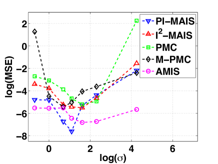
(a) Worst results.

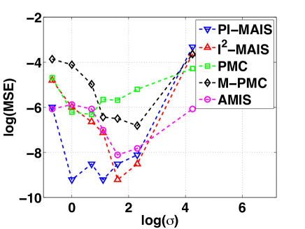
(b) Best results.

Figure 7: (Ex-Section-6.2) Graphical representation of the results in Table 12 (except for the last column): the curve $\log(\mbox{MSE})$ versus $\log(\sigma)$ with $\sigma\in\{0.5,1,2,3,5,10,70\}$ for the different methods, (a) worst and (b) best results.

The results are averaged $500$ over independent simulations, for each combination of parameters. Table 12 shows the smallest and highest MSE values obtained in the estimation of the expected value of the target, averaged between the two components of $E[{X}]$, achieved by the different methods. The smallest MSEs in each column (each $\sigma$) are highlighted in bold-face. PI-MAIS and I²-MAIS outperform the other techniques virtually for all the values of $\sigma$. In this example, AMIS also provides good results. Figure 7 show a graphical representation of the results in Table 12, with the exception of the last column.

Fig. 4 displays the initial (squares) and final (circles) configurations of the mean vectors of the proposals for the different algorithms, in one specific run. Since in Mixture PMC and AMIS the covariance matrices are also adapted, we show the shape of some proposals as ellipses representing approximately $85\%$ of probability mass. For, PMC we also depict a last resampling output with triangles, in order to show the loss in diversity. Unlike PMC, PI-MAIS ensures a better covering of the region of high probability.

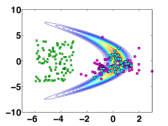
(a) PMC ($N=100$, $\sigma=1$)

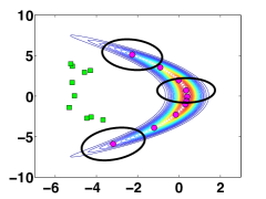
(b) Mixture PMC with 10 mixands ($\sigma=5$)

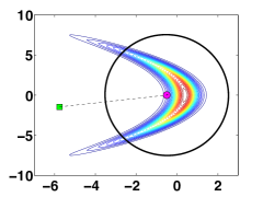
(c) AMIS ($\sigma=5$)

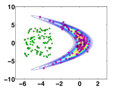
(d) PI-MAIS ($N=100$, $\lambda=3$)

Figure 4: Initial (squares) and final (circles) configurations of the mean vectors of the proposal densities for the banana-shaped target distribution, in one specific run for the different methods. The Mixture PMC (pmc-cappe08, ) and AMIS techniques (CORNUET12, ) also adapt the covariance matrices (the ellipses show approximately $85\%$ of the probability mass).

6.3 High dimensional target distribution

Let us consider again a mixture of isotropic Gaussians as target pdf, i.e.,

$$\bar{\pi}({\bf x})=\frac{1}{3}\sum_{k=1}^{3}\mathcal{N}({\bf x};{\bm{\nu}}_{k},{\bm{\Sigma}}_{k}),\quad{\bf x}\in\mathbb{R}^{D_{x}},$$ (40)

where ${\bm{\nu}}_{k}=[\nu_{k,1},\ldots,\nu_{k,D_{x}}]^{\top}$, and ${\bm{\Sigma}}_{k}=\chi_{k}^{2}{\bf I}_{D_{x}}$ for $k\in\{1,2,3\}$, with ${\bf I}_{D_{x}}$ being the $D_{x}\times D_{x}$ identity matrix. We set $\nu_{1,j}=-5$, $\nu_{2,j}=6$, $\nu_{3,j}=3$ for all $j=1,...,D_{x}$, and $\chi_{k}=8$ for all $k\in\{1,2,3\}$. The expected value of the target ${\pi}({\bf x})$ is then $E[{X_{j}}]=\frac{4}{3}$ for $j=1,\ldots,D_{x}$. In order to study the performance of the proposed scheme as the dimension of the state space increases, we vary the dimension of the state space in Eq. (40) testing different values of $D_{x}$ (with $2\leq D_{x}\leq 50$).

We consider the problem of approximating via Monte Carlo the expected value of the target density, and we compare the performance of different methods: (a) the standard PMC scheme (Cappe04, ), (b) $N$ parallel independent MH chains (Par-MH), (c) a standard Sequential Monte Carlo (SMC) scheme (Moral06, ) and (d) the proposed PI-MAIS method. We test the algorithms with $N\in\{100,500\}$. All the proposal pdfs involved in the experiments are Gaussians, with the same covariance matrices for all the techniques. The initial mean vectors in all techniques are selected randomly and independently as ${\bm{\mu}}_{n,0}\sim\mathcal{U}([-6\times 6]^{D_{x}})$ for $n=1,\ldots,N$.

Again, all the mentioned algorithms have been implemented in such a way that the number of total evaluations of the target is $E=2\cdot 10^{5}$. More specifically, in PI-MAIS, we use two sets of parameters: with $N=100$, $M=19$, $T=100$, and with $N=500$, $M=19$, $T=20$ in order to fulfill $E=(M+1)NT=2\cdot 10^{5}$ (see Section 5.4). The proposal pdf of the upper level of the hierarchical approach, $\varphi_{n}({\mathbf{x}}|{\bm{\mu}}_{n,t},{\bf\Lambda}_{n})$, are Gaussian pdfs with covariance matrices ${\bf\Lambda}_{n}=\lambda^{2}{\bf I}_{D_{x}}$ and $\lambda=10$. The proposal pdfs used in the lower importance sampling level, $q_{n,t}({\mathbf{x}}|{\bm{\mu}}_{n,t},{\bf C}_{n})$ are Gaussian pdfs with covariance matrices ${\bf C}_{n}=\sigma^{2}{\bf I}_{D_{x}}$ again with $\sigma=10$ (for a fair comparison with the other techniques). In PMC, Par-MH and SMC we use the same proposals with the same covariances and initial parameters. As described in App. C, in PMC the adaptation is carried out by resampling steps, in SMC an alternation of resampling and MH steps is performed whereas, in Par-MH, $N$ independent MH chains are carried out.

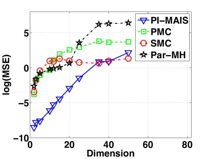
(a) $N=100$ and $E=2\cdot 10^{5}$.

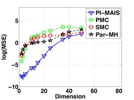
(b) $N=500$, keeping $E=2\cdot 10^{5}$.

Figure 8: (Ex-Section-6.3) The curve $\log(\mbox{MSE})$ as function of dimension of the problem, $D_{x}\in\{2,3,5,10,12,15,20,25,35,40,50\}$, for different methods. We test (a) $N=100$ and (b) $N=500$, keeping fixed the same number of evaluation of the target $E=2\cdot 10^{5}$. Hence the total number of iterations (of the different algorithms) is greater in Fig. 9(a) than in Fig. 9(b).

The results are averaged over $200$ independent simulations. Fig. 8 shows the log-MSE in the estimation of $E[{\bf X}]$ as a function of the dimension $D_{x}$ of the state-space. Fig. 8(a) compares the algorithms with $N=100$ proposal pdfs, whereas in Fig. 8(b) we have $N=500$, keeping fixed the number of total evaluations of the target $E=2\cdot 10^{5}$. We observe, as expected, the performance of all the methods degenerate as the dimension of the problem, $D_{x}$ increases, since we maintain fixed the computational cost $E=2\cdot 10^{5}$. PI-MAIS always provides the best results, with the exception for the cases corresponding to $N=100$ and $D_{x}=35,50$ where SMC obtains a lower MSE (for $N=100$ and $D_{x}=40$, they provide virtually the same MSE).

6.4 Localization problem in a wireless sensor network

We consider the problem of positioning a target in a $2$-dimensional space using range measurements. This problem appears frequently in localization applications in wireless sensor networks (Ali07, ; Ihler05, ; MartinoStatCo10, ). Namely, we consider a random vector $\textbf{X}=[X_{1},X_{2}]^{\top}$ to denote the target position in the plane $\mathbb{R}^{2}$. The position of the target is then a specific realization ${\bf X}={\bf x}$. The range measurements are obtained from $3$ sensors located at $\textbf{h}_{1}=[-10,2]^{\top}$, $\textbf{h}_{2}=[8,8]^{\top}$ and $\textbf{h}_{3}=[-20,-18]^{\top}$. The observation equations are given by

$$\begin{split}Y_{j}=a\log\left(\frac{||{\bf x}-{\bf h}_{j}||}{0.3}\right)+\Theta_{j},\quad j=1,\ldots,3,\\ \end{split}$$ (41)

where $\Theta_{j}$ are independent Gaussian variables with identical pdfs, $\mathcal{N}(\vartheta_{j};0,\omega^{2})$, $j=1,2$. We also consider a prior density over $\omega$, i.e., $\Omega\sim p(\omega)=\mathcal{N}(\omega;0,25)I(\omega>0),$ where $I(\omega>0)$ is $1$ if $\omega>0$ and $0$ otherwise. The parameter $A=a$ is also unknown and we again consider a Gaussian prior $A\sim p(a)=\mathcal{N}(a;0,25)$. Moreover, we also apply Gaussian priors over ${\bf X}$, i.e., $p(x_{i})=\mathcal{N}(x_{i};0,25)$ with $i=1,2$. Thus, the posterior pdf is

$$\bar{\pi}(x_{1},x_{2},a,\omega) = p(x_{1},x_{2},a,\omega|\textbf{y})$$

$$\propto \ell(\textbf{y}|x_{1},x_{2},a,\omega)p(x_{1})p(x_{2})p(a)p(\omega),$$

where ${\bf y}\in\mathbb{R}^{D_{y}}$ is the vector of received measurements. We simulate $d=30$ observations from the model ($D_{y}/3=10$ from each of the three sensors) fixing $x_{1}=3$, $x_{2}=3$, $a=-20$ and $\omega=5$. With $D_{y}=30$, the expected value of the target ($E[X_{1}]\approx 2.8749$, $E[X_{2}]\approx 3.0266$, $E[A]\approx 5.2344$, $E[\Omega]\approx 20.1582$) is quite close to the true values.

Our goal is computing the expected value of

$$(X_{1},X_{2},A,\Omega)\sim\bar{\pi}(x_{1},x_{2},a,\omega)$$

via Monte Carlo, in order to provide an estimate of the position of the target, the parameter $a$ and the standard deviation $\omega$ of the noise in the system. We apply PI-MAIS and three different PMC schemes (see example in Section 6.1, for a description), all using $N$ Gaussian proposals. We initialize the mean vectors so that they are randomly spread within the space of the variables of interest, i.e.,

$${\bm{\mu}}_{n,0}\sim\mathcal{N}({\bm{\mu}};{\bf 0},30^{2}{\bf I}_{4}),\quad n=1,...,N,$$

and the covariance matrices ${\bf C}_{n}=\mbox{diag}(\sigma_{n,1}^{2},\ldots,\sigma_{n,4}^{2}){\bf I}_{4}$ with $n=1,\ldots,N$. The values of the standard deviations $\sigma_{n,j}$ are chosen randomly for each Gaussian pdf. Specifically, $\sigma_{n,j}\sim\mathcal{U}([1,Q])$, $j=1,\ldots,4$, where we have considered three possible values for $Q$, i.e., $Q\in\{5,10,30\}$. For the adaptation process of PI-MAIS, we consider also Gaussian proposals with covariance matrices ${\bf\Lambda}_{n}=\lambda^{2}{\bf I}_{2}$ and $\lambda\in\{5,10,70\}$. We also try different non-isotropic diagonal covariance matrices, i.e, ${\bf\Lambda}_{n}=\textrm{diag}(\lambda_{n,1}^{2},\lambda_{i,2}^{2})$, where $\lambda_{n,j}\sim\mathcal{U}([1,30])$.

For a fair comparison, all the techniques have been simulated with sets of parameters that yield the same number of target evaluations, fixed to $E=2\cdot 10^{5}$. In PI-MAIS, we have chosen parameters $N=100$, $M=\{1,19,99\}$, $T=\{20,100,1000\}$. The PMC algorithms has been simulated with $N=100$ and $T=2000$. The MSE of the different estimators (averaged over $3000$ independent runs) are provided in Table 13 and the $\log(\mbox{MSE})$ in Figure 6(b). PI-MAIS outperforms always PMC when $\sigma_{n,j}\sim\mathcal{U}([1,5])$ and $\sigma_{n,j}\sim\mathcal{U}([1,10])$ whereas PMC provides better results for $\sigma_{n,j}\sim\mathcal{U}([1,30])$. Therefore, the results show jointly the robustness and flexibility of the proposed PI-MAIS technique.

7 Conclusions

In this work, we have introduced a layered (i.e., hierarchical) framework for designing adaptive Monte Carlo methods. In general terms, we have shown that such a hierarchical interpretation lies behind the good performance of two well-known algorithms; a random walk proposal within an MH scheme and the standard PMC method. Furthermore, we have used this approach to introduce a novel class of adaptive importance sampling (AIS) schemes. The novel class of AIS algorithms employs the determinist mixture (DM) idea (Owen00, ; Veach95, ) in order to reduce the variance of the resulting IS estimators. We have extended the use of the DM strategy with respect to other algorithms available in the literature, providing a more general and flexible framework. From an estimation perspective, this framework includes different schemes proposed in literature (CORNUET12, ; APIS15, ) as special cases, although they differ to an extent in terms of the employed adaptation procedure. Our framework also contains several other sampling schemes considering full or partial DM approaches. Finally, we have discussed several aspects of the trade-offs in terms of the computational cost and advantages due to improved accuracy of the resulting estimators. Numerical comparisons with different algorithms on benchmark models have confirmed the benefit of the layered adaptive sampling approaches.

Appendix A Consistency of GAMIS estimators

First of all, we remark that the complete analysis should take in account the chosen adaptive procedure since, in general, the adaptation uses the information of previous weighted samples. However, in this work we consider an adaption procedure completely independent of the estimation steps, as clarified in Sections 3.4-5.1. This simplifies substantially the analysis as described in Section 5.1.

The consistency of the global estimators in Eq. (29) provided by GAMIS can be considered when number of samples per time step ($M\times N$) and the number of iterations of the algorithm ($T$) grow to infinity. For some exhaustive studies of specific cases, see the analysis in [47, 17] and [34]. Here we provide some brief arguments for explaining why $\hat{I}_{T}$ and ${\hat{Z}}_{T}$ obtained by a GAMIS scheme are, in general, consistent. Let us assume that $q_{n,t}$’s have heavier tails than $\bar{\pi}({\bf x})\propto\pi({\bf x})$. Note that the global estimator $\hat{I}_{T}$ can be seen as a result of a static batch MIS estimator involving $L$ different mixture-proposals $\Phi_{n,t}({\bf x})$ and $J=NMT$ total number of samples. The weights $w_{n,t}^{(m)}$ built using $\Phi_{n,t}({\bf x})$ in the denominator of the IS ratio are suitable importance weights yielding consistent estimators, as explained in detail in AppendixB. Hence, for a finite number of iterations $T<\infty$, when $M\rightarrow\infty$ (or $N\rightarrow\infty$), the consistency can be guaranteed by standard IS arguments, since it is well known that $\hat{Z}_{T}\to Z$ and $\hat{I}_{T}\to I$ as $M\to\infty$, or $N\to\infty$ [47].

Furthermore, for $T\rightarrow\infty$ and $N,M<\infty$, we have a convex combination, given in Eq. (31), of conditionally independent (consistent but biased) IS estimators [47]. Indeed, although in an adaptive scheme the proposals depend on the previous configurations of the population, the samples drawn at each iteration are conditionally independent of the previous ones, and independent of each other drawn at the same iteration. The bias is due to unknown $Z$ (see Eq. (4)), and hat $\hat{Z}_{T}$ is used to replace $Z$. However, $\hat{Z}_{T}\to Z$ as $T\to\infty$, as discussed in [47, Chapter 14]: hence, $\hat{I}_{T}$ is asymptotically unbiased as $T\to\infty$.

Appendix B Importance sampling with multiple proposals

Recall that our goal is computing efficiently the integral $I=\frac{1}{Z}\int_{\mathcal{X}}f({\bf x})\pi({\bf x})d{\bf x}$ where $f$ is any square-integrable function (w.r.t. $\bar{\pi}({\bf x})$) of ${\bf x}$, and $Z=\int_{\mathcal{X}}\pi({\bf x})d{\bf x}<\infty$ with $\pi({\bf x})\geq 0$ for all ${\bf x}\in\mathcal{X}\subseteq\mathbb{R}^{D_{x}}$. Let us assume that we have two proposal pdfs, $q_{1}({\bf x})$ and $q_{2}({\bf x})$, from which we intend to draw $M_{1}$ and $M_{2}$ samples respectively:

$${\bf x}_{1}^{(1)},\ldots,{\bf x}_{1}^{(M_{1})}\sim q_{1}({\bf x})\quad\quad\mbox{ and }\quad\quad{\bf x}_{2}^{(1)},\ldots,{\bf x}_{2}^{(M_{2})}\sim q_{2}({\bf x}).$$

There are at least two procedures to build a joint IS estimator: the standard multiple importance sampling (MIS) approach and the full deterministic mixture (DM-MIS) scheme.

B.1 Standard IS approach

The simplest approach [47, Chapter 14] is computing the classical IS weights:

$$w_{1}^{(i)}=\frac{\pi({\bf x}_{1}^{(i)})}{q_{1}({\bf x}_{1}^{(i)})},\quad w_{2}^{(k)}=\frac{\pi({\bf x}_{2}^{(k)})}{q_{2}({\bf x}_{2}^{(k)})},$$ (42)

with $i=1,\ldots,M_{1}$ and $k=1,\ldots,M_{2}$. The IS estimator is then built by normalizing them jointly, i.e., computing

$$\hat{I}_{IS}=\frac{1}{S_{tot}}\left(\sum_{i=1}^{M_{1}}w_{1}^{(i)}f({\bf x}_{1}^{(i)})+\sum_{k=1}^{M_{2}}w_{2}^{(k)}f({\bf x}_{2}^{(k)})\right),$$ (43)

where $S_{tot}=\sum_{i=1}^{M_{1}}w_{1}^{(i)}+\sum_{k=1}^{M_{2}}w_{2}^{(k)}$. For $J>2$ proposal pdfs and ${\bf x}_{j}^{(1)},\ldots,{\bf x}_{j}^{(M_{j})}\sim q_{j}({\bf x})$, for $j=1,\ldots,J$, we have

$$\left\{\begin{split}w_{j}^{(m_{j})}&=\frac{\pi({\bf x}_{j}^{(m_{j})})}{q_{j}({\bf x}_{j}^{(m_{j})})},\quad\mbox{ and }\\ \hat{I}_{IS}&=\frac{1}{\sum_{n=1}^{J}\sum_{m_{j}=1}^{M_{j}}w_{j}^{(m_{j})}}\sum_{j=1}^{J}\sum_{m_{j}=1}^{M_{j}}w_{j}^{(m_{j})}f({\bf x}_{j}^{(m_{j})}).\end{split}\right.$$

In this case, $S_{tot}=\sum_{n=1}^{J}\sum_{m_{j}=1}^{M_{j}}w_{j}^{(m_{j})}$.

B.2 Deterministic mixture approach

An alternative approach is based on the deterministic mixture sampling idea [46, 50, 22]. Considering $N=2$ proposals $q_{1}$, $q_{2}$, and setting

$$\mathcal{Z}=\left\{{\bf x}_{1}^{(1)},\ldots,{\bf x}_{1}^{(M_{1})},{\bf x}_{2}^{(1)},\ldots,{\bf x}_{2}^{(M_{2})}\right\},$$

with ${\bf x}_{j}^{(m_{j})}\in\mathbb{R}^{D_{x}}$ ($n\in\{1,2\}$ and $1\leq m_{j}\leq M_{j}$), the weights are now defined as

$$w_{j}^{(m_{j})}=\frac{\pi({\bf x}_{j}^{(m_{j})})}{\frac{M_{1}}{M_{1}+M_{2}}q_{1}({\bf x}_{j}^{(m_{j})})+\frac{M_{2}}{M_{1}+M_{2}}q_{2}({\bf x}_{j}^{(m_{j})})}.$$ (44)

In this case, the complete proposal is considered to be a mixture of $q_{1}$ and $q_{2}$, weighted according to the number of samples drawn from each one. Note that, unlike in the standard procedure for sampling from a mixture, a deterministic and fixed number of samples are drawn from each proposal in the DM approach [22]. It can be shown that the set $\mathcal{Z}$ of samples drawn in this deterministic way is distributed according to the mixture $q({\bf z})=\frac{M_{1}}{M_{1}+M_{2}}q_{1}({\bf z})+\frac{M_{2}}{M_{1}+M_{2}}q_{2}({\bf z})$ [45, Chapter 9, Section 11]. The DM estimator is finally given by

$$\hat{I}_{DM}=\frac{1}{S_{tot}}\sum_{j=1}^{2}\sum_{m_{j}=1}^{M_{j}}{w_{j}^{(m_{j})}f({\bf x}_{j}^{(m_{j})})},$$ (45)

where $S_{tot}=\sum_{j=1}^{2}\sum_{m_{j}=1}^{M_{j}}w_{j}^{(m_{j})}$ and the $w_{j}^{(m_{j})}$ are given by (44). For $J>2$ proposal pdfs, the DM estimator can also be easily generalized:

$$\left\{\begin{split}w_{i}^{(m_{i})}&=\frac{\pi({\bf x}_{i}^{(m_{i})})}{\sum_{j=1}^{J}{\frac{M_{j}}{M_{tot}}q_{j}({\bf x}_{j}^{(m_{j})})}},\quad\mbox{ and }\\ \hat{I}_{DM}&=\frac{1}{\sum_{n=1}^{J}\sum_{m_{j}=1}^{M_{j}}w_{j}^{(m_{j})}}\sum_{j=1}^{J}\sum_{m_{j}=1}^{M_{j}}w_{j}^{(m_{j})}f({\bf x}_{j}^{(m_{j})}),\end{split}\right.$$

with $i=1,\ldots,J$, $M_{tot}=M_{1}+M_{2}+\ldots+M_{J}$ and $S_{tot}=\sum_{j=1}^{J}\sum_{m_{j}=1}^{M_{j}}w_{j}^{(m_{j})}$. On the one hand, the DM approach is more efficient than the IS method, thus providing a better performance in terms of a reduced variance of the corresponding estimator, as shown in the following section. On the other hand, it needs to evaluate every proposal $M_{tot}$ times instead of only $M_{j}$ times (in the standard MIS procedure), and therefore is more costly from a computational point of view. However, this increased computational cost is negligible when the proposal is much cheaper to evaluate than the target, as it often happens in practical applications.

B.3 Convex combination of partial IS estimators

Regardless the type of weights employed in the IS scheme (either as in Eq. (42) or as in Eq. (44)), the resulting estimators can be written as convex combination of simpler ones. First of all, let us consider again the use of $J=2$ proposals, $q_{1}$ and $q_{2}$. We draw $M_{j}$ samples from each one, ${\bf x}_{j}^{(1)},\ldots,{\bf x}_{j}^{(M_{j})}\sim q_{j}({\bf x})$, with $j\in\{1,2\}$. The two partial sums of the weights corresponding only to the samples drawn from $q_{1}$ and $q_{2}$, are given by $S_{1}=\sum_{i=1}^{M_{1}}w_{1}^{(i)}$ and $S_{2}=\sum_{k=1}^{M_{2}}w_{2}^{(k)}$. The partial IS estimators, obtained by considering only one proposal pdf, are $\hat{I}_{1}=\sum_{i=1}^{M_{1}}\bar{w}_{1}^{(i)}f({\bf x}_{1}^{(i)})$ and $\hat{I}_{2}=\sum_{k=1}^{M_{2}}\bar{w}_{2}^{(k)}f({\bf x}_{2}^{(k)})$ where the normalized weights are $\bar{w}_{1}^{(i)}=\frac{w_{1}^{(i)}}{S_{1}}$ and $\bar{w}_{2}^{(k)}=\frac{w_{2}^{(k)}}{S_{2}}$, respectively. The complete IS estimator, taking into account the $M_{1}+M_{2}$ samples jointly, is

$$\hat{I}_{tot} = \frac{1}{S_{1}+S_{2}}\left(S_{1}\hat{I}_{1}+S_{2}\hat{I}_{2}\right)$$ (46)

$$= \frac{S_{1}}{S_{1}+S_{2}}\hat{I}_{1}+\frac{S_{2}}{S_{1}+S_{2}}\hat{I}_{2}.$$

This procedure can be easily extended for $J>2$ different proposal pdfs, obtaining the complete estimator as the convex combination of the $N$ partial estimators:

$$\begin{split}\hat{I}_{tot}&=\frac{\sum_{j=1}^{J}{S_{j}\hat{I}_{j}}}{\sum_{j=1}^{J}{S_{j}}},\\ \hat{Z}_{tot}&=\frac{1}{\sum_{j=1}^{J}M_{j}}\sum_{j=1}^{J}{S_{j}}=\frac{1}{\sum_{j=1}^{J}M_{j}}\sum_{j=1}^{J}M_{j}{\hat{Z}_{j}},\end{split}$$ (47)

where ${\bf x}_{j}^{(1)},\ldots,{\bf x}_{j}^{(M_{j})}\sim q_{j}({\bf x})$, $\hat{I}_{j}=\sum_{k=1}^{M_{j}}{w_{j}^{(k)}f({\bf x}_{j}^{(k)})}$, $S_{j}=\sum_{k=1}^{M_{j}}{w_{j}^{(k)}}$ and $\hat{Z}_{j}=\frac{1}{M_{j}}\sum_{k=1}^{M_{j}}w_{j}^{(k)}$.

Appendix C Hierarchical interpretation of PMC

The standard Population Monte Carlo (PMC) [12] method can be interpreted as using a hierarchical procedure. Although it is possible to recognize the two different layers, there are some differences w.r.t. the hierarchical procedure in Section 3. The first one is that in PMC the generation of ${\bm{\mu}}$’s is not independent of the previously generated ${\bf x}$’s. The second one is that the prior is instead $h({\bm{\mu}})=\hat{\pi}_{t}^{(N)}({\bm{\mu}})$, where $\hat{\pi}_{t}^{(N)}$ is an approximation of the measure of $\bar{\pi}({\bm{\mu}})$ obtained using the previously generated samples ${\bf x}$’s (in the second level of the hierarchical approach). More specifically, a standard PMC method [12] is an adaptive importance sampler using a population of proposals $q_{1}$, $\ldots$, $q_{N}$. PMC consists of the following steps, given an initial set, ${\bm{\mu}}_{1,0}$, $\ldots$, ${\bm{\mu}}_{N,0}$, of mean vectors:

1. For $t=0,\ldots,T-1:$

   1. Draw ${\bf x}_{n,t}\sim q_{n,t}({\bf x}|{\bm{\mu}}_{n,t},{\bf C}_{n})$, for $n=1,\ldots,N$.

   2. Assign to each sample ${\bf x}_{n,t}$ the weights,

      $$w_{n,t}=\frac{\pi({\bf x}_{n,t})}{q_{n,t}({\bf x}_{n,t}|{\bm{\mu}}_{n,t},{\bf C}_{n})}.$$ (48)

   3. Resampling: draw $N$ independent samples ${\bm{\mu}}_{n,t+1}$, $n=1,\ldots,N$, according to the particle approximation

      $$\hat{\pi}_{t}^{(N)}({\bm{\mu}}|{\bf x}_{1:N,t})=\frac{1}{\sum_{n=1}^{N}w_{n,t}}\sum_{n=1}^{N}w_{n,t}\delta({\bm{\mu}}-{\bf x}_{n,t}),$$ (49)

      where we have denoted ${\bf x}_{1:N,t}=[{\bf x}_{1,t},\ldots,{\bf x}_{N,t}]^{\top}$. Note that each ${\bm{\mu}}_{n,t+1}\in\{{\bf x}_{1,t},\ldots,{\bf x}_{N,t}\}$, for all $n$.

2. Return all the pairs $\{{\bf x}_{n,t},w_{n,t}\}$, $n=1,\ldots,N$ and $t=0,\ldots,T-1$.

Fixing an iteration $t$, the generating procedure used in one iteration of the standard PMC method can be cast in the hierarchical formulation:

1. Draw $N$ samples ${\bm{\mu}}_{1,t},\ldots,{\bm{\mu}}_{N,t}$ from $\hat{\pi}_{t-1}^{(N)}({\bm{\mu}}|{\bf x}_{1:N,t-1})$.

2. Draw ${\bf x}_{n,t}\sim q_{n,t}({\bf x}|{\bm{\mu}}_{n,t},{\bf C}_{n})$, for $n=1,\ldots,N$.

Note that $\hat{\pi}_{t-1}^{(N)}$ plays the role of the prior $h$ in the hierarchical scheme above. Differently from the novel proposed scheme, the two levels of hierarchical procedure are not independent since the pdf $\hat{\pi}_{t}^{(N)}({\bm{\mu}}|{\bf x}_{1:N,t})$ depends on the samples drawn in the lower level. Furthermore, $\hat{\pi}_{t}^{(N)}$ also varies with $t$ and $N$, whereas in our procedure we consider a fixed prior $h$. However, note that $\hat{\pi}_{t}^{(N)}$ is an empirical measure approximation of ${\bar{\pi}}$ that improves when $N$ grows. An equivalent formulation of the hierarchical scheme for PMC is given below, involving a probability of generating a new mean ${\bm{\mu}}$ given the previous ones ${\bm{\mu}}_{1:N,t-1}=[{\bm{\mu}}_{1,t-1},\ldots,{\bm{\mu}}_{N,t-1}]^{\top},$ denoted as $K_{t}^{(N)}({\bm{\mu}}|{\bm{\mu}}_{1:N,t-1})$.

C.1 Distribution after one resampling step

Consider the $t$-th iteration of PMC. Let us define as

$${\bf m}_{\neg n}=[{\bf x}_{1,t},\ldots,{\bf x}_{n-1,t},{\bf x}_{n+1,t},\ldots,{\bf x}_{N,t}]^{\top},$$

the vector containing all the generated samples except for the $n$-th. Let us also denote as ${\bm{\mu}}_{i,t+1}\in\{{\bf x}_{1,t}\ldots,{\bf x}_{N,t}\}$, a generic mean vector, i.e. $i\in\{1,\ldots,N\}$ at the iteration $t+1$, after applying one resampling step (i.e., a multinomial sampling according to the normalized weights). Hence, the distribution of ${\bm{\mu}}$ given the previous means ${\bm{\mu}}_{1:N,t-1}$ is

$$\begin{split}&K_{t+1}^{(N)}({\bm{\mu}}_{i,t+1}|{\bm{\mu}}_{1,t},\dots,{\bm{\mu}}_{N,t})=\\ &=\int_{\mathcal{X}^{N}}\hat{\pi}_{t}^{(N)}({\bm{\mu}}_{i,t+1}|{\bf x}_{1:N,t})\left[\prod_{n=1}^{N}{q_{n,t}({\bf x}_{n,t}|{\bm{\mu}}_{n,t},{\bf C}_{n})}\right]d{\bf x}_{1:N,t},\end{split}$$ (50)

where $\hat{\pi}_{t}^{(N)}({\bm{\mu}}|{\bf x}_{1:N,t})$ is given in Eq. (49). For simplicity, below we denote

$$q_{n}({\bf x})=q_{n,t}({\bf x}|{\bm{\mu}}_{n,t},{\bf C}_{n}),\quad\mbox{ and }{\bm{\mu}}={\bm{\mu}}_{i,t}.$$

Then, after some straightforward rearrangements, Eq. (50) can be rewritten as

$$K_{t+1}^{(N)}({\bm{\mu}}|{\bm{\mu}}_{1,t},\dots,{\bm{\mu}}_{N,t})=$$

$$= \sum_{j=1}^{N}\left(\int_{\mathcal{X}^{N-1}}\frac{\pi({\bf x}_{j,t})}{\sum_{n=1}^{N}{\frac{\pi({\bf x}_{n,t})}{q_{n}({\bf x}_{n,t})}}}\left[\prod_{\begin{subarray}{c}n=1\\ n\neq j\end{subarray}}^{N}{q_{n}({\bf x}_{n,t})}\right]d{\bf m}_{\neg j}\right)\delta({\bm{\mu}}-{\bf x}_{j,t}).$$

Finally, we can write

$$K_{t+1}^{(N)}({\bm{\mu}}|{\bm{\mu}}_{1,t},\dots,{\bm{\mu}}_{N,t})=$$

$$\pi({\bm{\mu}})\sum_{j=1}^{N}\left({\int_{\mathcal{X}^{N-1}}\frac{1}{N\hat{Z}}\left[\prod_{\begin{subarray}{c}n=1\\ n\neq j\end{subarray}}^{N}q_{n}({\bf x}_{n,t})\right]d{\bf m}_{\neg j}}\right),$$ (51)

where $\hat{Z}=\frac{1}{N}\sum_{n=1}^{N}\frac{\pi({\bf x}_{n})}{q_{n}({\bf x}_{n})}$ is the estimate of the normalizing constant of the target obtained using the classical IS weights. The hierarchical formulation of PMC can be rewritten as:

1. Draw $N$ samples ${\bm{\mu}}_{1,t},\ldots,{\bm{\mu}}_{N,t}$ from $K_{t}^{(N)}({\bm{\mu}}|{\bm{\mu}}_{1:N,t-1})$ in Eq. (50) or (51).

2. Draw ${\bf x}_{n,t}\sim q_{n,t}({\bf x}|{\bm{\mu}}_{n,t},{\bf C}_{n})$, for $n=1,\ldots,N$.

When $N\to\infty$, then $\hat{Z}\to Z$ [47], and thus $K_{t}^{(N)}({\bm{\mu}}|{\bm{\mu}}_{1:N,t-1})\to\frac{1}{Z}\pi({\bm{\mu}})=\bar{\pi}({\bm{\mu}})$, for all $t=1\ldots,T$. Namely, when $N$ grows, the hierarchical scheme above tends to have $h({\bm{\mu}})={\bar{\pi}}({\bm{\mu}})$ as prior in the upper level. Figures 5 show three different examples of the conditional pdf $K_{t}^{(N)}$ (obtained via numerical approximation) for a fixed $t$ and different $N\in\{2,20,1000\}$. We can observe that $K_{t}^{(N)}$ becomes closer to the target $\bar{\pi}$ (depicted in solid line) as $N$ grows.

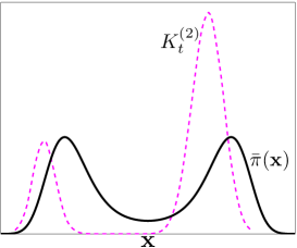
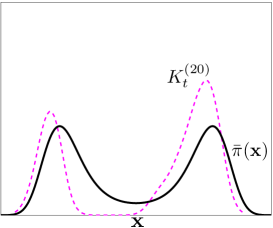
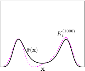
Figure 5: Examples of $K_{t}^{(N)}({\bm{\mu}}|{\bm{\mu}}_{1:N,t-1})$ (approximated numerically and shown with dashed line) and a bimodal target pdf ${\bar{\pi}}({\bf x})$ (solid line), fixing an iteration $t$ within a PMC method and for different $N$: (a) $N=2$, (b) $N=20$ and (c) $N=1000$.

C.1.1 Differences between PMC and MAIS algorithms

In the Markov adaptive importance sampling (MAIS) schemes described in Section 5, since we are using MCMC methods for drawing from $h({\bm{\mu}})={\bar{\pi}}({\bm{\mu}})$, actually we have also a current prior $K_{t}^{(N)}({\bm{\mu}}_{1:N,t}|{\bm{\mu}}_{1:N,t-1})$, determined for the kernels of the considered MCMC algorithms. For instance, in PI-MAIS we have

$$K_{t}^{(N)}({\bm{\mu}}_{1:N,t}|{\bm{\mu}}_{1:N,t-1})=\prod_{n=1}^{N}A_{n}({\bm{\mu}}_{n,t}|{\bm{\mu}}_{n,t-1}),$$

where $A_{n}({\bm{\mu}}_{n,t}|{\bm{\mu}}_{n,t-1})$ is the kernel of the $n$-th chain. Unlike in PMC, since we are using ergodic chains with invariant pdf ${\bar{\pi}}$, we know that $K_{t}^{(N)}({\bm{\mu}}_{1:N,t}|{\bm{\mu}}_{1:N,t-1})\rightarrow\prod_{n=1}^{N}{\bar{\pi}}({\bm{\mu}}_{n})$ for $t\rightarrow\infty$, with a fixed $N$. Whereas PMC requires to increase $N$ for obtaining the same result.

Algorithm			$\sigma=0.5$	$\sigma=1$	$\sigma=2$	$\sigma=5$	$\sigma=10$	$\sigma=70$	$\sigma_{n,j}\sim\mathcal{U}([1,10])$
	$\lambda=5$	$M=99,T=20$	1.2760	0.5219	0.5930	0.0214	0.0139	0.1815	0.0107
		$M=19,T=100$	0.2361	0.1205	0.0422	0.0087	0.0140	0.1868	0.0052
		$M=1,T=1000$	0.1719	0.0019	0.0155	0.0103	0.0273	0.3737	0.0070
	$\lambda=10$	$M=99,T=20$	1.0195	0.1546	0.2876	0.0178	0.0133	0.1789	0.0098
		$M=19,T=100$	0.1750	0.0120	0.0528	0.0086	0.0136	0.1856	0.0050
PI-MAIS ($N=100$)		$M=1,T=1000$	0.1550	0.0021	0.0020	0.0095	0.0252	0.3648	0.0066
	$\lambda=70$	$M=99,T=20$	16.9913	5.5790	1.4925	0.0382	0.0128	0.1834	0.0252
		$M=19,T=100$	2.6693	0.9182	0.1312	0.0147	0.0143	0.1844	0.0120
		$M=1,T=1000$	0.3014	0.1042	0.0136	0.0115	0.0267	0.3697	0.0093
	$\lambda_{n,j}\sim\mathcal{U}([1,10])$	$M=99,T=20$	1.0707	0.5364	0.3523	0.0199	0.0121	0.1919	0.0094
		$M=19,T=100$	0.2481	0.0595	0.1376	0.0075	0.0144	0.1899	0.0049
		$M=1,T=1000$	0.1046	0.0037	0.0045	0.0099	0.0274	0.3563	0.0065
Static standard MIS	$\Phi_{n,t}({\bf x})=q_{n,t}({\bf x})$		29.56	41.95	64.51	2.17	0.0147	0.1914	4.55
Static partial DM-MIS	$\Phi_{n,t}({\bf x})=\phi_{t}({\bf x})$		29.28	47.74	75.22	0.2424	0.0124	0.1789	0.0651
AMIS [15]	(best results)		124.22	121.21	100.23	0.8640	0.0121	0.0136	0.7328
	(worst results)		125.43	123.38	114.82	16.92	0.0128	18.66	13.49
PMC [12]			112.99	114.11	47.97	2.34	0.0559	2.41	0.3017
PMC with partial DM-MIS	$N=100$, $T=2000$		111.92	107.58	26.86	0.6731	0.0744	2.42	0.0700
Mixture PMC [11]			110.17	113.11	50.23	2.75	0.0521	2.57	0.6194
Parallel Indep. MH chains	$N=100$,$T=2000$		1.6910	1.7640	1.8832	1.4133	0.2969	0.5475	7.3446

Table 9: (Ex-Sect 6.1) MSE of the estimator of the $E[{\bf X}]$ (first component) with the initialization In1. For all the techniques, the total number of evaluations of the target is $E=2\cdot 10^{5}$. We recall that, in AMIS [15], $N=1$ and $\Phi_{1,t}({\bf x})=\xi_{1}({\bf x})$. The last row corresponds to the application of $N=100$ (as in PI-MAIS) parallel MH chains where the random walk proposals have covariance matrices ${\bf C}=\sigma^{2}{\bf I}_{2}$. The lengths of the chains, as well as of the PMC runs, is $T=2000$ for keeping $E=2\cdot 10^{5}$. For the techniques which adapt the covariance matrices of the proposal pdfs, the values of $\sigma$ have been employed as initial scale values for the covariance matrices. For AMIS, we show the best and worst results obtained testing different combinations of $M$ and $T=\frac{E}{M}$. The best results, in each column, are highlighted with bold-faces.

Algorithm			$\sigma=0.5$	$\sigma=1$	$\sigma=2$	$\sigma=5$	$\sigma=10$	$\sigma=70$	$\sigma_{n,j}\sim\mathcal{U}([1,10])$
										$\lambda=5$	$M=99,T=20$	0.6096	0.0657	0.0023	0.0056	0.0124	0.1768	0.0051
		$M=19,T=100$	0.2878	0.0358	0.0010	0.0050	0.0127	0.1802	0.0038
		$M=1,T=1000$	0.1244	0.0011	0.0014	0.0091	0.0242	0.3510	0.0064
	$\lambda=10$	$M=99,T=20$	0.9236	0.0543	0.0021	0.0062	0.0137	0.1815	0.0054
		$M=19,T=100$	0.2294	0.0077	0.0012	0.0054	0.0132	0.1890	0.0044
PI-MAIS ($N=100$)		$M=1,T=1000$	0.0786	0.0042	0.0014	0.0086	0.0256	0.3503	0.0066
	$\lambda=70$	$M=99,T=20$	5.9889	0.3662	0.0082	0.0089	0.0140	0.1841	0.0093
		$M=19,T=100$	1.6670	0.0871	0.0045	0.0080	0.0139	0.1971	0.0074
		$M=1,T=1000$	0.2579	0.0134	0.0024	0.0097	0.0258	0.3543	0.0082
	$\lambda_{n,j}\sim\mathcal{U}([1,10])$	$M=99,T=20$	0.5623	0.0417	0.0025	0.0059	0.0124	0.1848	0.0056
		$M=19,T=100$	0.2704	0.0204	0.0011	0.0048	0.0136	0.1726	0.0037
		$M=1,T=1000$	0.0750	0.0014	0.0013	0.0089	0.0247	0.3540	0.0066
Static standard MIS	$\Phi_{n,t}({\bf x})=q_{n,t}({\bf x})$		12.00	9.40	10.26	7.67	0.5443	0.1764	4.37
Static partial DM-MIS	$\Phi_{n,t}({\bf x})=\phi_{t}({\bf x})$		10.14	0.9469	0.0139	0.0100	0.0146	0.1756	0.0106
AMIS [15]	(best results)		113.97	112.70	107.85	44.93	0.7404	0.0141	31.02
	(worst results)		116.66	115.62	111.83	70.62	9.43	18.62	58.63
PMC [12]			111.54	110.78	90.21	2.29	0.0631	2.42	0.3082
PMC with partial DM-MIS	$N=100$, $T=2000$		23.16	7.43	7.56	0.6420	0.0720	2.37	0.0695
Mixture PMC [11]			25.43	10.68	6.29	0.6142	0.0727	2.55	0.1681
Parallel Indep. MH chains	$N=100$,$T=2000$		1.3813	1.3657	1.2942	1.0178	0.3644	1.0405	5.3211

Table 10: (Ex-Sect 6.1) MSE of the estimator of the expected value (first component). For all the techniques, the total number of evaluations of the target is again $E=2\cdot 10^{5}$. In this case, we have applied the initialization In2, differently from Table 9. The best results, in each column, are highlighted with bold-faces.

Algorithm			$\sigma=0.5$	$\sigma=1$	$\sigma=2$	$\sigma=5$	$\sigma=10$	$\sigma=70$	$\sigma_{n,j}\sim\mathcal{U}([1,10])$
	$\lambda=5$	$M=99,T=20$	0.0388	0.0120	0.0070	0.0002	0.0001	0.0016	0.0001
		$M=19,T=100$	0.0031	0.0013	0.0004	0.0001	0.0001	0.0017	0.0001
		$M=1,T=1000$	0.0016	0.0001	0.0001	0.0001	0.0002	0.0031	0.0001
	$\lambda=10$	$M=99,T=20$	0.0217	0.0046	0.0040	0.0001	0.0001	0.0016	0.0002
		$M=19,T=100$	0.0019	0.0002	0.0005	0.0001	0.0001	0.0017	0.0001
PI-MAIS ($N=100$)		$M=1,T=1000$	0.0016	0.0001	0.0001	8 ${\bf\cdot 10^{-5}}$	0.0002	0.0031	0.0001
	$\lambda=70$	$M=99,T=20$	6.3732	0.2713	0.0226	0.0003	0.0001	0.0016	0.0002
		$M=19,T=100$	0.1082	0.0114	0.0019	0.0001	0.0001	0.0017	0.0001
		$M=1,T=1000$	0.0038	0.0009	0.0001	0.0001	0.0002	0.0033	0.0001
	$\lambda_{n,j}\sim\mathcal{U}([1,10])$	$M=99,T=20$	0.0350	0.0101	0.0043	0.0001	0.0001	0.0015	0.0001
		$M=19,T=100$	0.0029	0.0007	0.0010	8 ${\bf\cdot 10^{-5}}$	9 $\cdot 10^{-5}$	0.0017	9 ${\bf\cdot 10^{-5}}$
		$M=1,T=1000$	0.0014	0.0001	${\bf 9\cdot 10^{-5}}$	0.0001	0.0002	0.0036	0.0001
Static standard MIS	$\Phi_{n,t}({\bf x})=q_{n,t}({\bf x})$		3.94 $\cdot 10^{4}$	7.12 $\cdot 10^{7}$	1.07 $\cdot 10^{3}$	0.0113	0.0001	0.0016	0.2190
Static partial DM-MIS	$\Phi_{n,t}({\bf x})=\phi_{t}({\bf x})$		9.51$\cdot 10^{8}$	4.60 $\cdot 10^{5}$	15.34	0.0016	0.0001	0.0016	0.0005
AMIS [15]	(best results)		15.92	15.66	12.81	0.0069	8 ${\bf\cdot 10^{-5}}$	0.0001	0.0002
	(worst results)		15.97	15.92	14.87	0.4559	0.0001	1.62	0.0084
PMC [12]			33.53	17.10	14.42	0.4249	0.0015	0.0016	0.3542
PMC with partial DM-MIS	$N=100$, $T=2000$		15.85	14.31	1.81	0.0402	0.0002	0.0016	0.0004
Mixture PMC [11]			14.51	12.09	3.56	0.0287	0.0002	0.0015	0.0010

Table 11: (Ex-Sect 6.1) MSE of the estimator of the normalizing constant $Z$ with the initialization In1. For all the techniques, the total number of evaluations of the target is $E=2\cdot 10^{5}$. The smallest MSE for each $\sigma$ is bold-faced.

Algorithm		$\sigma=0.5$	$\sigma=1$	$\sigma=2$	$\sigma=3$	$\sigma=5$	$\sigma=10$	$\sigma=70$	$\sigma_{i,j}\sim\mathcal{U}([1,20])$
PI-MAIS	Worst	0.0083	0.0081	0.0012	0.0005	0.0050	0.0126	0.1126	0.0218
	Best	0.0025	0.0001	0.0002	0.0001	0.0002	0.0003	0.0361	0.0004
I2-MAIS	Worst	0.0335	0.0227	0.0053	0.0044	0.0041	0.0096	0.2130	0.0181
	Best	0.0082	0.0025	0.0013	0.0008	0.0001	0.0002	0.0265	0.0003
PMC [12]	Worst	0.0670	0.0461	0.0209	0.0093	0.0055	0.0072	9.4749	0.1065
	Best	0.0210	0.0164	0.0069	0.0016	0.0015	0.0011	0.0262	0.0026
Mixture PMC [11]	Worst	3.5772	0.0113	0.0044	0.0066	0.0174	0.0267	0.0913	0.0103
	Best	0.0092	0.0020	0.0018	0.0035	0.0034	0.0055	0.0138	0.0025
AMIS [15]	Worst	0.0040	0.0039	0.0040	0.0016	0.0011	0.0012	0.0035	0.0013
	Best	0.0023	0.0028	0.0023	0.0009	0.0003	0.0004	0.0023	0.0007

Table 12: (Ex-Section-6.2) Bi-dimensional banana-shaped distribution example: Best and worst results in terms of MSE, obtained with the different techniques for different values of $\sigma$. The smallest MSE for each $\sigma$ is bold-faced.

Algorithm			$\sigma_{i,j}\sim\mathcal{U}([1,5])$	$\sigma_{i,j}\sim\mathcal{U}([1,10])$	$\sigma_{i,j}\sim\mathcal{U}([1,30])$
PI-MAIS	$\lambda=5$	$M=99,T=20$	0.3819	0.3508	0.3626
		$M=19,T=100$	0.0728	0.0738	0.0710
		$M=1,T=1000$	0.0173	0.0164	0.0171
	$\lambda=10$	$M=99,T=20$	0.5701	0.5943	0.5605
		$M=19,T=100$	0.1389	0.1429	0.1425
		$M=1,T=1000$	0.0401	0.0408	0.0393
	$\lambda_{i,j}\sim\mathcal{U}([1,30])$	$M=99,T=20$	0.3758	0.3795	0.4028
		$M=19,T=100$	0.0741	0.0793	0.0771
		$M=1,T=1000$	0.0169	0.0167	0.0162
PMC [12]			0.0642	0.4345	0.1533
PMC with partial DM-MIS	$N=100$, $T=2000$		0.0524	0.3163	0.0817
Mixture PMC [11]			0.0577	0.2870	0.4083

Table 13: (Ex-Sect 6.4) MSE of the estimator of $E[(X_{1},X_{2},A,\Omega)]$ using different techniques, keeping constant the total number of target evaluation, $E=2\ 10^{5}$. The best results, in each column, are highlighted with bold-faces.

References

- [1] A. M. Ali, K. Yao, T. C. Collier, E. Taylor, D. Blumstein, and L. Girod. An empirical study of collaborative acoustic source localization. Proc. Information Processing in Sensor Networks (IPSN07), Boston, April 2007.
- [2] C. Andrieu, N. de Freitas, A. Doucet, and M. Jordan. An introduction to MCMC for machine learning. Machine Learning, 50:5–43, 2003.
- [3] C. Andrieu, A. Doucet, and R. Holenstein. Particle Markov chain Monte Carlo methods. Journal of the Royal Statistical Society B, 72(3):269–342, 2010.
- [4] C. Andrieu and J. Thoms. A tutorial on adaptive mcmc. Statistics and Computing, 18:343 373, 2015.
- [5] F. Beaujean and Caldwell A. Initializing adaptive importance sampling with Markov chains. arXiv:1304.7808, 2013.
- [6] Z. I. Botev and D. P. Kroese. An efficient algorithm for rare-event probability estimation, combinatorial optimization, and counting. Methodology and Computing in Applied Probability, 10(4):471–505, December 2008.
- [7] Z. I. Botev, P. L Ecuyer, and B. Tuffin. Markov chain importance sampling with applications to rare event probability estimation. Statistics and Computing, 23:271–285, 2013.
- [8] A. Brockwell, P. Del Moral, and A. Doucet. Interacting Markov chain Monte Carlo methods. The Annals of Statistics, 38(6):3387–3411, 2010.
- [9] M. F. Bugallo, L. Martino, and J. Corander. Adaptive importance sampling in signal processing. Digital Signal Processing, 47:36–49, 2015.
- [10] A. Caldwell and C. Liu. Target density normalization for Markov Chain Monte Carlo algorithms. arXiv:1410.7149, 2014.
- [11] O. Cappé, R. Douc, A. Guillin, J. M. Marin, and C. P. Robert. Adaptive importance sampling in general mixture classes. Statistics and Computing, 18:447–459, 2008.
- [12] O. Cappé, A. Guillin, J. M. Marin, and C. P. Robert. Population Monte Carlo. Journal of Computational and Graphical Statistics, 13(4):907–929, 2004.
- [13] S. Chib and I. Jeliazkov. Marginal likelihood from the metropolis-hastings output. Journal of the American Statistical Association, 96:270–281, 2001.
- [14] N. Chopin. A sequential particle filter for static models. Biometrika, 89:539–552, 2002.
- [15] J. M. Cornuet, J. M. Marin, A. Mira, and C. P. Robert. Adaptive multiple importance sampling. Scandinavian Journal of Statistics, 39(4):798–812, December 2012.
- [16] R. Craiu, J. Rosenthal, and C. Yang. Learn from thy neighbor: Parallel-chain and regional adaptive MCMC. Journal of the American Statistical Association, 104(448):1454–1466, 2009.
- [17] G.R. Douc, J.M. Marin, and C. Robert. Convergence of adaptive mixtures of importance sampling schemes. Annals of Statistics, 35:420–448, 2007.
- [18] G.R. Douc, J.M. Marin, and C. Robert. Minimum variance importance sampling via population Monte Carlo. ESAIM: Probability and Statistics, 11:427–447, 2007.
- [19] A. Doucet and A. M. Johansen. A tutorial on particle filtering and smoothing: fifteen years later. technical report, 2008.
- [20] A. Doucet and X. Wang. Monte Carlo methods for signal processing. IEEE Signal Processing Magazine, 22(6):152–170, Nov. 2005.
- [21] V. Elvira, L. Martino, D. Luengo, and M. Bugallo. Efficient multiple importance sampling estimators. IEEE Signal Processing Letters, 22(10):1757–1761, 2015.
- [22] V. Elvira, L. Martino, D. Luengo, and M. F. Bugallo. Generalized multiple importance sampling. arXiv:1511.03095, 2015.
- [23] P. Fearnhead and B. M. Taylor. An adaptive Sequential Monte Carlo sampler. Bayesian Analysis, 8(2):411–438, 2013.
- [24] W. J. Fitzgerald. Markov chain Monte Carlo methods with applications to signal processing. Signal Processing, 81(1):3–18, January 2001.
- [25] N. Friel and J. Wyse. Estimating the model evidence: a review. arXiv:1111.1957, 2011.
- [26] C. J. Geyer. Markov Chain Monte Carlo maximum likelihood. Computing Science and Statistics: Proceedings of the 23rd Symposium on the Interface, pages 156–163, 1991.
- [27] H. Haario, E. Saksman, and J. Tamminen. An adaptive Metropolis algorithm. Bernoulli, 7(2):223–242, April 2001.
- [28] A. T. Ihler, J. W. Fisher, R. L. Moses, and A. S. Willsky. Nonparametric belief propagation for self-localization of sensor networks. IEEE Transactions on Selected Areas in Communications, 23(4):809–819, April 2005.
- [29] P. Jacob, C. P. Robert, and M. H. Smith. Using parallel computation to improve Independent Metropolis-Hastings based estimation. Journal of Computational and Graphical Statistics, 3(20):616–635, 2011.
- [30] F. Liang, C. Liu, and R. Caroll. Advanced Markov Chain Monte Carlo Methods: Learning from Past Samples. Wiley Series in Computational Statistics, England, 2010.
- [31] R. Liesenfeld and J. F.Richard. Improving MCMC, using efficient importance sampling. Computational Statistics and Data Analysis, 53:272–288, 2008.
- [32] J. S. Liu, F. Liang, and W. H. Wong. The multiple-try method and local optimization in metropolis sampling. Journal of the American Statistical Association, 95(449):121–134, March 2000.
- [33] D. Luengo and L. Martino. Fully adaptive Gaussian mixture Metropolis-Hastings algorithm. Proceedings of IEEE International Conference on Acoustics, Speech, and Signal Processing (ICASSP), 2013.
- [34] J. M. Marin, P. Pudlo, and M. Sedki. Consistency of the adaptive multiple importance sampling. arXiv:1211.2548, 2012.
- [35] E. Marinari and G. Parisi. Simulated tempering: a new Monte Carlo scheme. Europhysics Letters, 19(6):451–458, July 1992.
- [36] L. Martino, V. Elvira, D. Luengo, A. Artes, and J. Corander. Orthogonal MCMC algorithms. IEEE Workshop on Statistical Signal Processing (SSP), pages 364–367, June 2014.
- [37] L. Martino, V. Elvira, D. Luengo, A. Artes, and J. Corander. Smelly parallel MCMC chains. IEEE International Conference on Acoustics, Speech, and Signal Processing (ICASSP), 2015.
- [38] L. Martino, V. Elvira, D. Luengo, and J. Corander. An adaptive population importance sampler: Learning from the uncertanity. IEEE Transactions on Signal Processing, 63(16):4422–4437, 2015.
- [39] L. Martino, V. Elvira, D. Luengo, and J. Corander. MCMC-driven adaptive multiple importance sampling. Interdisciplinary Bayesian Statistics Springer Proceedings in Mathematics & Statistics (Chapter 8), 118:97–109, 2015.
- [40] L. Martino and J. Míguez. A generalization of the adaptive rejection sampling algorithm. Statistics and Computing, 21(4):633–647, July 2011.
- [41] E. F. Mendes, M. Scharth, and R. Kohn. Markov Interacting Importance Samplers. arXiv:1502.07039, 2015.
- [42] P. Del Moral, A. Doucet, and A. Jasra. Sequential Monte Carlo samplers. Journal of the Royal Statistical Society: Series B (Statistical Methodology), 68(3):411–436, 2006.
- [43] R. Neal. MCMC using ensembles of states for problems with fast and slow variables such as Gaussian process regression. arXiv:1101.0387, 2011.
- [44] R. M. Neal. Annealed importance sampling. Statistics and Computing, 11(2):125–139, 2001.
- [45] A. Owen. Monte Carlo theory, methods and examples. http://statweb.stanford.edu/owen/mc/, 2013.
- [46] A. Owen and Y. Zhou. Safe and effective importance sampling. Journal of the American Statistical Association, 95(449):135–143, 2000.
- [47] C. P. Robert and G. Casella. Monte Carlo Statistical Methods. Springer, 2004.
- [48] C. Schäfer and N. Chopin. Sequential Monte Carlo on large binary sampling spaces. Statistics and Computing, 23(2):163–184, 2013.
- [49] J. Skilling. Nested sampling for general Bayesian computation. Bayesian Analysis, 1(4):833–860, June 2006.
- [50] E. Veach and L. Guibas. Optimally combining sampling techniques for Monte Carlo rendering. In SIGGRAPH 1995 Proceedings, pages 419–428, 1995.
- [51] M.P. Wand and M.C. Jones. Kernel Ssoothing. Chapman and Hall, 1994.
- [52] X. Wang, R. Chen, and J. S. Liu. Monte Carlo Bayesian signal processing for wireless communications. Journal of VLSI Signal Processing, 30:89–105, 2002.
- [53] M. D. Weinberg. Computing the Bayes factor from a Markov chain Monte Carlo simulation of the posterior distribution. arXiv:0911.1777, 2010.
- [54] X. Yuan, Z. Lu, and C. Z. Yue. A novel adaptive importance sampling algorithm based on Markov chain and low-discrepancy sequence. Aerospace Science and Technology, 29:253–261, 2013.