Existence of a weak solution to a fluid-elastic structure interaction problem with the Navier slip boundary condition

Abstract

We study a nonlinear, moving boundary fluid-structure interaction (FSI) problem between an incompressible, viscous Newtonian fluid, modeled by the 2D Navier-Stokes equations, and an elastic structure modeled by the shell or plate equations. The fluid and structure are coupled via the Navier slip boundary condition and balance of contact forces at the fluid-structure interface. The slip boundary condition might be more realistic than the classical no-slip boundary condition in situations, e.g., when the structure is “rough”, and in modeling FSI dynamics near, or at a contact. Cardiovascular tissue and cell-seeded tissue constructs, which consist of grooves in tissue scaffolds that are lined with cells, are examples of “rough” elastic interfaces interacting with an incompressible, viscous fluid. The problem of heart valve closure is an example of a FSI problem with a contact involving elastic interfaces. We prove the existence of a weak solution to this class of problems by designing a constructive proof based on the time discretization via operator splitting. This is the first existence result for fluid-structure interaction problems involving elastic structures satisfying the Navier slip boundary condition.

1 Introduction

We study a nonlinear, moving boundary fluid-structure interaction (FSI) problem between a viscous, incompressible Newtonian fluid, modeled by the Navier-Stokes equations, and an elastic shell or plate. The fluid and structure are coupled through two coupling conditions: the Navier slip boundary condition and the continuity of contact forces at the fluid-structure interface. The Navier slip boundary condition states that the difference, i.e., the slip between the tangential components of the fluid and structure velocities is proportional to the tangential component of the fluid normal stress evaluated at the fluid-structure interface, while the normal components of the fluid and structure velocities are continuous. The main motivation for using the Navier slip boundary condition comes from fluid-structure interaction (FSI) problems involving elastic structures with “rough” boundaries, and from studying FSI problems near a contact.

FSI problems involving elastic structures with rough boundaries appear, for example when studying FSI between blood flow and cardiovascular tissue, whether natural or bio-artificial, which is lined with cells that are in direct contact with blood flow. Bio-artificial vascular tissue constructs (i.e., vascular grafts) often times involve cells seeded on tissue scaffolds with grooved microstructure, which interacts with blood flow. See Figure 1. To filter out the small scales of the rough fluid domain boundary, effective boundary conditions based on the Navier slip condition have been used in various applications, see e.g., a review paper by Mikelić [41], and [21, 6, 31]. Instead of using the no-slip condition at the groove-scale on the rough boundary, the Navier slip condition is applied at the smooth boundary instead.

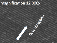
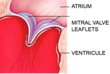
Figure 1: Two examples of fluid-elastic structure interaction problems where the Navier slip condition may be more appropriate. Left: An image of a nano-patterned film surface for vascular tissue engineering [58] giving rise to a “rough” surface interacting with blood flow. The grooves in this tissue construct are to be lined with cells, producing a bio-artificial vascular graft for a replacement of diseased arteries. The grooves are perpendicular to the direction of blood flow. Right: A sketch of a closed mitral valve interacting with blood flow. Modeling the contact between leaflets with the no-slip condition gives rise to leaky valves due to the no-slip condition paradox in collision of smooth bodies [49, 26, 27, 52].

Another motivation for using the Navier slip boundary condition comes from studying problems near or at a contact (or collision). It has been shown recently that the no-slip condition is not a realistic physical condition to model contact between smooth rigid bodies immersed in an incompressible fluid [49, 26, 27, 52]. It was shown that two smooth rigid bodies cannot touch each other if the no-slip boundary condition is considered. One solution to this no-collision paradox is to consider bodies with “non-smooth” boundaries, in which case collisions can occur [18]. The other explanation for the no-collision paradox is that the no-slip boundary condition does not describe near-contact dynamics well, and a new model and/or a different boundary condition, such as for example, the Navier slip boundary condition, need to be employed to model contact between bodies/structures interacting while immersed in an incompressible, viscous fluid [47]. Examples include applications in cardiovascular sciences, for example, modeling the closure of heart valves. It is well known that numerical simulation of heart valve closure suffers from the “numerical” leakage of blood through a “closed” heart valve whenever the no-slip boundary condition is used. Different kinds of “gap” boundary conditions have been used to get around this difficulty, see e.g., [15]. Considering the Navier slip boundary condition near or at the closure would provide a more realistic modeling of the problem.

From the mathematical analysis point of view, the fist step in the direction of studying the Navier slip boundary condition near or at a contact was made by Neustupa and Penel [47] who proved that when the no-slip boundary condition is replaced with the slip boundary condition, collision can occur for a prescribed movement of rigid bodies. Recently, Gérard-Varet and Hillairet considered an FSI problem involving a movement of a rigid solid immersed in an incompressible Navier-Stokes flow with the slip boundary condition and proved the existence of a weak solution up to collision [19]. In a subsequent work [20] they proved that prescribing the slip boundary condition on both the rigid body boundary and the boundary of the domain, allows collision of the rigid body with the boundary. The existence of a global weak solution which permits collision of a “smooth” rigid body with a “smooth” fluid domain boundary was proved in [11]. For completeness, we also mention several recent works where the slip boundary condition was considered in various existence results for FSI problems involving rigid bodies and Newtonian fluids [46, 48, 57]. All the above-mentioned works consider FSI between rigid bodies and an incompressible, viscous fluid. To the best of our knowledge there are no existence results for non-linear moving boundary FSI problems involving elastic structures satisfying the Navier slip boundary condition. The present work is the first existence result involving the Navier slip boundary condition for a fluid-structure interaction problem with elastic structures.

Classical FSI problems with the no-slip boundary condition have been extensively studied from both the analytical and numerical point of view (see e.g. [5, 17, 42] and the references within). Earlier works have focused on problems in which the coupling between the fluid and structure was calculated at a fixed fluid domain boundary, see [16], and [2, 3, 35], where an additional nonlinear coupling term was added and calculated at a fixed fluid interface. A study of well-posedness for FSI problems between an incompressible, viscous fluid and an elastic/viscoelastic structure satisfying the no-slip boundary condition, with the coupling evaluated at a moving interface, started with the result of daVeiga [4], where existence of a strong solution was obtained locally in time for an interaction between a $2D$ fluid and a $1D$ viscoelastic string, assuming periodic boundary conditions. This result was extended by Lequeurre in [37, 38], where the existence of a unique, local in time, strong solution for any data, and the existence of a global strong solution for small data, was proved in the case when the structure was modeled as a clamped viscoelastic beam.

D. Coutand and S. Shkoller proved existence, locally in time, of a unique, regular solution for an interaction between a viscous, incompressible fluid in $3D$ and a $3D$ structure, immersed in the fluid, where the structure was modeled by the equations of linear elasticity satisfying no-slip at the interface [13]. In the case when the structure (solid) is modeled by a linear wave equation, I. Kukavica et al. proved the existence, locally in time, of a strong solution, assuming lower regularity for the initial data [32, 33, 29]. A similar result for compressible flows can be found in [34]. In [51] Raymod et al. considered a FSI problem between a linear elastic solid immersed in an incompressible viscous fluid, and proved the existence and uniqueness of a strong solution. All the above mentioned existence results for strong solutions are local in time. Recently, in [30] a global existence result for small data was obtained for a similar moving boundary FSI problem but with additional interface and structure damping terms.

In the context of weak solutions incorporating the no-slip condition, the following results have been obtained. Existence of a weak solution for a FSI problem between a $3D$ incompressible, viscous fluid and a $2D$ viscoelastic plate was shown by Chambolle et al. in [10], while Grandmont improved this result in [22] to hold for a $2D$ elastic plate. These results were extended to a more general geometry in [36], and to a non-Newtonian shear dependent fluid in [40]. In these works existence of a weak solution was proved for as long as the elastic boundary does not touch ”the bottom” (rigid) portion of the fluid domain boundary.

Muha and Čanić recently proved the existence of a weak solution to a class of FSI problems modeling the flow of an incompressible, viscous, Newtonian fluid flowing through a 2D cylinder whose lateral wall was modeled by either the linearly viscoelastic, or by the linearly elastic Koiter shell equations [42], assuming nonlinear coupling at the deformed fluid-structure interface. These results were extended by the same authors to a 3D FSI problem involving a cylindrical Koiter shell [43], and to a semi-linear cylindrical Koiter shell [45]. The main novelty in these works was a design of a constructive existence proof based on the Lie operator splitting scheme, which has been used in numerical simulation of several FSI problems [24, 7, 42, 8, 28, 40], and has proven to be a robust method for a design of constructive existence proofs for an entire class of FSI problems.

In the present work a further non-trivial extension of the Lie operator splitting scheme is introduced to deal with the Navier slip boundary condition and with the non-zero longitudinal displacement of the structure. Dealing with the Navier slip condition and non-zero longitudinal displacement introduces several mathematical difficulties. In contrast with the no-slip boundary condition which “transmits” the regularizing mechanism by the viscous fluid dissipation onto the fluid-structure interface, in the Navier slip condition the tangential components of the fluid and structure velocities are no longer continuous, and thus information is lost in the tangential direction. As a result, new compactness arguments had to be designed in the existence proof to control the tangential velocity components at the interface. The compactness arguments are based on Simon’s characterization of compactness in $L^{2}(0,T;B)$ spaces [53], and on interpolation of the classical Sobolev spaces with real exponents $H^{s}$ (or alternatively Nikolskii spaces $N^{s,p}\cite[cite]{[\@@bibref{}{Simon2}{}{}]})$. This is new. If we had worked with continuous energy estimate, we would have been able to obtain structure regularity in the standard space $L^{\infty}(0,T;H^{2}(\Gamma))$. The time-discretization via operator splitting, however, enabled us to obtain an additional estimate in time that is due to the dissipative term in the backward Euler approximation of the time derivative of the structure velocity. The uniform boundedness of this term enabled us to obtain structure regularity in $H^{s}(0,T;H^{2}(\Gamma))$, $s<1/2$. This was crucial for the existence proof. This approach in general brings new information about the time-behavior of weak solutions to the elastic structure problems.

Furthermore, to deal with the non-zero longitudinal displacement and keep the behavior of fluid-structure interface “under control”, we had to consider higher-order terms in the structure model given by the bending rigidity of shells. The linearly elastic membrane model was not tractable. Due to the non-zero longitudinal displacement additional nonlinearities appear in the problem that track the geometric quantities such as the fluid-structure interface surface measure, the interface tangent and normal, and the change in the moving fluid domain measure (given by the Jacobian of the ALE mapping mapping the moving domain onto a fixed, reference domain). These now appear explicitly in the weak formulation of the problem, and cause various difficulties in the analysis. This is one of the reasons why our existence result is local in time, i.e., it holds for the time interval $(0,T)$ for which we can guarantee that the fluid domain does not degenerate in the sense that the ALE mapping remains injective in time as the fluid domain moves, and the Jacobian of the ALE mapping remains strictly positive, see Figure 3. Therefore, in this manuscript we prove the existence, locally in time, of a weak solution, to a nonlinear moving-boundary problem between an incompressible, viscous Newtonian fluid and an elastic shell or plate, satisfying the Navier slip condition at the fluid-structure interface, and balance of forces at the fluid-structure interface.

2 Problem description

We study the flow of an incompressible, viscous fluid through a 2D fluid domain whose boundary contains an elastic, thin structure. The fluid and structure are fully coupled through two coupling conditions: the Navier slip boundary condition, and the dynamic coupling condition describing the balance of forces at the elastic structure interface. The flow is driven by the data, which includes the case of the time-dependent dynamic pressure data prescribed at the “inlet and outlet” portion of the fixed boundary, denoted in Figure 2 as $\Gamma_{1}$ and $\Gamma_{3}$. The reference fluid domain, denoted by $\Omega\subset{\mathbb{R}}^{2}$, is considered to be a polygon with angles less than of equal to $\pi$, see Figure 2. If we denote by $\Gamma_{i},i=0,\dots,m$ the faces of $\Omega$, without the loss of generality we can assume that $\Gamma_{0}$ is compliant, and $\Gamma_{1},\dots,m$ is the rigid portion. We denote the rigid portion by ${\Sigma=\bigcup_{i=1}^{m}\overline{\Gamma_{i}}}$, and the compliant portion by $\Gamma=\Gamma_{0}=(0,L)$.

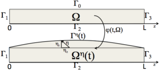
Figure 2: An example of fluid and structure domains.

As the fluid flows through the compliant domain, the elastic part of the boundary deforms, giving rise to a time-dependent fluid domain which is not known a priori. We denote by $\boldsymbol{\varphi}(t,.):\Omega\to{\mathbb{R}}^{2}$, $t\in[0,T)$ the time-dependent deformation of the fluid domain determined by the interaction between fluid flow and the elastic part of the fluid domain boundary. We will be assuming that $\boldsymbol{\varphi}$ is such that the rigid portion $\Sigma$ of the fluid domain remains fixed, and that the fluid domain does not degenerate in the sense that the elastic structure does not touch any part of the boundary during deformation. More precisely, we will be assuming that $\boldsymbol{\varphi}$ is a $C^{1}$ diffeomorphism such that

$$\boldsymbol{\varphi}_{|\Sigma}={\bf id}\ {\rm and}\ {\rm det}\nabla\boldsymbol{\varphi}(t,{\bf x})>0,\ (t,{\bf x})\in[0,T)\times\overline{\Omega}.$$

We denote the displacement of the elastic part of the boundary $\Gamma_{0}$ by $\boldsymbol{\eta}(t,{\bf x})=\boldsymbol{\varphi}(t,{\bf x})-{\bf x},\;{\bf x}\in\Gamma_{0}$. Since $\Gamma_{0}$ can be identified by the interval $(0,L)$, as mentioned above, $\boldsymbol{\eta}$ is defined as a mapping $\boldsymbol{\eta}:[0,T)\times[0,L]\to{\mathbb{R}}^{2}$, with

$$\boldsymbol{\eta}(t,z)=(\eta_{z}(t,z),\eta_{r}(t,z)),\;z\in[0,L],\;\eta(0)=\partial_{z}\eta(0)=\eta(L)=\partial_{z}\eta(L)=0.$$ (1)

Here $\eta_{z}$ and $\eta_{r}$ denote the tangential and normal components of displacement with respect to the reference configuration $\Gamma_{0}$, respectively, and the last set of conditions in (1) state that the elastic structure is clamped at the points at which it meets the rigid portion of the boundary $\Sigma$. We denote by $\Omega^{\eta}(t)=\boldsymbol{\varphi}(t,\Omega)$ the deformed fluid domain at time $t$, and by $\Gamma^{\eta}(t)=\boldsymbol{\varphi}(t,\Gamma_{0})$ the corresponding deformed elastic part of the boundary of $\Omega^{\eta}(t)$. We chose to include $\boldsymbol{\eta}$ as a superscript in the notation for the deformed fluid domain and for the deformed elastic structure to emphasize that they both depend on one of the unknowns in the problem, which is the structure displacement $\boldsymbol{\eta}$. The following notation will be useful in subsequent calculations. The surface element of the deformed structure will be denoted by:

$$d\Gamma^{\eta}=\sqrt{(1+\partial_{z}\eta_{z}(t,z))^{2}+(\partial_{r}\eta_{r}(t,z))^{2}}dz=S^{\eta}(t,z)dz,$$

the tangent vector to the deformed structure will be denoted by ${\boldsymbol{\tau}}^{\eta}(t,z)=\partial_{z}\boldsymbol{\varphi}^{\eta}(t,z)$, and the outer unit normal on $\Gamma^{\eta}(t)$ at point $\boldsymbol{\varphi}(t,z)$ will be denoted by $\boldsymbol{\nu}^{\eta}(t,z)$.

The fluid. The fluid flow is governed by the Navier-Stokes equations for an incompressible, viscous fluid defined on the family of time-dependent domains $\Omega^{\eta}(t)$:

$$\left.\begin{array}[]{rcl}\rho_{F}(\partial_{t}{\bf u}+{\bf u}\cdot\nabla{\bf u})&=&\nabla\cdot\boldsymbol{\sigma},\\ \nabla\cdot{\bf u}&=&0,\end{array}\right\}\ {\rm in}\ \Omega^{\eta}(t),\ t\in(0,T),$$ (2)

where $\rho_{F}$ denotes the fluid density, ${\bf u}$ is the fluid velocity, $\boldsymbol{\sigma}=-p{\bf I}+2\mu{\bf D}({\bf u})$ is the fluid Cauchy stress tensor, $p$ is the fluid pressure, $\mu$ is the kinematic viscosity coefficient, and ${\bf D}({\bf u})=\frac{1}{2}(\nabla{\bf u}+\nabla^{\tau}{\bf u})$ is the symmetrized gradient of ${\bf u}$.

The approach presented in this manuscript can handle different types of boundary conditions prescribed on the rigid boundary $\Sigma$. More precisely, on each face $\Gamma_{i}$ of the rigid boundary $\Sigma$ we prescribe one of the following four types of boundary conditions:

1. Dynamic pressure: $p+\frac{\rho_{F}}{2}|{\bf u}|^{2}=P_{i},{\bf u}\cdot\boldsymbol{\tau}=0$, prescribed on $\Gamma_{i},i\in I$,

2. Velocity (no-slip): ${\bf u}={\bf 0}$, prescribed on $\Gamma_{i},i\in II$,

3. The Navier slip boundary condition: ${\bf u}\cdot\boldsymbol{\nu}=0,{\bf u}\cdot\boldsymbol{\tau}+\alpha_{i}\boldsymbol{\sigma}\boldsymbol{\nu}\cdot\boldsymbol{\tau}=0$, prescribed on $\Gamma_{i},i\in III$,

4. The symmetry boundary condition: ${\bf u}\cdot\boldsymbol{\nu}=0,\;\partial_{\nu}u_{\tau}=0$, prescribed on $\Gamma_{i},i\in IV$,

where $I$, $II$, $III$ and $IV$ denote the subsets of the set of indices $\{1,\dots,m\}$ such that the boundary condition of type $1$, $2$, $3$ or $4$ is satisfied. We note that non-homogeneous boundary conditions can also be handled with additional care.

The problem is supplemented with the initial condition:

$$\begin{array}[]{c}{\bf u}(0,.)={\bf u}_{0}.\end{array}$$ (3)

To close the problem, it remains to specify the boundary conditions on the elastic part of the boundary $\Gamma^{\eta}(t)$. For this purpose we introduce the elastodynamics equations modeling the motion of the elastic structure, and the two-way coupling between the structure and the fluid motion.

The structure. The elasto-dynamics of thin structure $\Gamma^{\eta}(t)$ will be given in terms of displacement with respect to the reference configuration $\Gamma=\Gamma_{0}=(0,L)$ (Lagrangian formulation). To include different shell models, we formulate the elastodynamics problem in terms of a general continuous, self-adjoint, coercive, linear operator ${\cal L}_{e}$, defined on $H_{0}^{2}(0,L)$, for which there exists a constant $c>0$ such that

$$\left<{\cal{L}}_{e}\boldsymbol{\eta},\boldsymbol{\eta}\right>\geq c\|\boldsymbol{\eta}\|^{2}_{H_{0}^{2}(\Gamma)},\quad\forall\boldsymbol{\eta}\in H_{0}^{2}(\Gamma),$$ (4)

where $\left<\cdot,\cdot\right>$ is the duality pairing between $H_{0}^{2}$ and $H^{-2}$. The structure elastodynamics problem is then given by:

$$\rho_{S}h\partial_{tt}\boldsymbol{\eta}=-{\cal L}_{e}\boldsymbol{\eta}+{\bf f},\quad z\in\Gamma=(0,L),\ t\in(0,T),$$ (5)

$$\boldsymbol{\eta}(t,0)=\partial_{z}\boldsymbol{\eta}(t,0)=\boldsymbol{\eta}(t,L)=\partial_{z}\boldsymbol{\eta}(t,L)=0,\; t\in(0,T),$$ (6)

$$\boldsymbol{\eta}(0,z)=\boldsymbol{\eta}_{0},\;\partial_{t}\boldsymbol{\eta}(0,z)={\bf v}_{0},; z\in\Gamma=(0,L).$$

where $\rho_{S}$ is the structure density, $h$ the elastic shell thickness, ${\bf f}$ is linear force density acting on the shell, $\boldsymbol{\eta}=(\eta_{z},\eta_{r})$ is the shell displacement, and $\boldsymbol{\eta}_{0}$ and ${\bf v}_{0}$ are the initial structure displacement and the initial structure velocity, respectively.

The fluid and structure equations are coupled via the following two sets of coupling conditions:

• The  kinematic  coupling condition (Navier slip condition):

  $$\begin{array}[]{l}{\rm Continuity\ of\ normal\ velocity\;on\;}\Gamma^{\eta}(t):\\ \displaystyle{\partial_{t}\boldsymbol{\eta}(t,z)\cdot\boldsymbol{\nu}^{\eta}(t,z)}=\boldsymbol{u}(\boldsymbol{\varphi}(t,z))\cdot\boldsymbol{\nu}^{\eta}(t,z),\quad(t,z)\in(0,T)\times\Gamma,\\ \\ {\rm The\ slip\ condition\ between\ the\ fluid\ and\ thin\ structure\;on\;}\Gamma^{\eta}(t):\\ \displaystyle{(\partial_{t}\boldsymbol{\eta}(t,z)-{\bf u}(\boldsymbol{\varphi}(t,z)))\cdot\boldsymbol{\tau}^{\eta}(t,z)}\\ \displaystyle{=\alpha\boldsymbol{\sigma}\big{(}\phi(t,z)\big{)}\boldsymbol{\nu}^{\eta}(t,z)\cdot\boldsymbol{\tau}}^{\eta}(t,z),\quad(t,z)\in(0,T)\times\Gamma.\end{array}$$ (7)

• The  dynamic  coupling condition:

  $$\rho_{S}h\partial_{tt}\boldsymbol{\eta}(t,z)=-{\mathcal{L}}_{e}\boldsymbol{\eta}(t,z)-S^{\eta}(t,z)\boldsymbol{\sigma}\big{(}\boldsymbol{\varphi}(t,z)\big{)}\boldsymbol{\nu}^{\eta}(t,z),\;(t,z)\in(0,T)\times\Gamma,$$ (8)

  stating that the structure interface elastodynamics is driven by the jump in the normal stress across the interface, where we have assumed, without the loss of generality, that the normal stress on the outside of the structure is equal to zero. The term $S^{\eta}$, which multiplies the normal fluid stress $\boldsymbol{\sigma}\boldsymbol{\nu}^{\eta}$, is the Jacobian of the transformation between the Eulerian and Lagrangian formulations of the fluid and structure problems, respectively.

Notice that there is no pressure contribution in the slip condition (7). The pressure contributes only through the dynamic coupling condition (8).

In summary, we study the following problem.

Find $({\bf u},\boldsymbol{\eta})$ such that the following holds: The fluid equations: $$\left.\begin{array}[]{rcl}\rho_{F}(\partial_{t}{\bf u}+{\bf u}\cdot\nabla{\bf u})&=&\nabla\cdot\boldsymbol{\sigma},\\ \nabla\cdot{\bf u}&=&0,\end{array}\right\}\ {\rm in}\ \Omega^{\eta}(t),\ t\in(0,T);$$ (9) The elastic structure (boundary conditions on $(0,T)\times\Gamma$): $\displaystyle\rho_{S}h\partial_{tt}\boldsymbol{\eta}(t,z)+{\mathcal{L}}_{e}\boldsymbol{\eta}(t,z)$ $\displaystyle=$ $\displaystyle-S^{\eta}(t,z)\boldsymbol{\sigma}\big{(}\boldsymbol{\varphi}(t,z)\big{)}\boldsymbol{\nu}^{\eta}(t,z),$ (10) $\displaystyle\displaystyle{\partial_{t}\boldsymbol{\eta}(t,z)\cdot\boldsymbol{\nu}^{\eta}(t,z)}$ $\displaystyle=$ $\displaystyle\boldsymbol{u}(\boldsymbol{\varphi}(t,z))\cdot\boldsymbol{\nu}^{\eta}(t,z),$ (11) $\displaystyle\displaystyle{(\partial_{t}\boldsymbol{\eta}(t,z)-{\bf u}(\boldsymbol{\varphi}(t,z))\cdot\boldsymbol{\tau}^{\eta}(t,z)}$ $\displaystyle=$ $\displaystyle\alpha\boldsymbol{\sigma}\big{(}\boldsymbol{\varphi}(t,z)\big{)}\boldsymbol{\nu}^{\eta}(t,z)\cdot\boldsymbol{\tau}^{\eta}(t,z),$ (12) with $$\boldsymbol{\eta}(t,0)=\partial_{z}\boldsymbol{\eta}(t,0)=\boldsymbol{\eta}(t,L)=\partial_{z}\boldsymbol{\eta}(t,L)=0,\;t\in(0,T);$$ Boundary conditions on $\Sigma$: $$\begin{array}[]{rl}p+\frac{\rho_{F}}{2}|{\bf u}|^{2}=P_{i},\;{\bf u}\cdot\boldsymbol{\tau}=0&{\rm on}\;\Gamma_{i},\;i\in I,\\ {\bf u}={\bf 0}&{\rm on}\;\Gamma_{i},\;i\in II,\\ {\bf u}\cdot\boldsymbol{\nu}=0,{\bf u}\cdot\boldsymbol{\tau}+\alpha_{i}\boldsymbol{\sigma}\boldsymbol{\nu}\cdot\boldsymbol{\tau}=0&{\rm on}\;\Gamma_{i},\;i\in III,\\ {\bf u}\cdot{\bf n}=0,\;\partial_{\nu}u_{\tau}=0&{\rm on}\;\Gamma_{i},\;i\in IV;\end{array}$$ (13) with $u_{\tau}$ denoting the tangental component of velocity $\bf u$. Initial conditions: $${\bf u}(0,.)={\bf u}_{0},\;\boldsymbol{\eta}(0,.)=\boldsymbol{\eta}_{0},\;\partial_{t}\boldsymbol{\eta}(0,.)={\bf v}_{0}.$$ (14) The initial data must satisfy the following compatibility conditions:

• The initial fluid velocity must satisfy:

  $$\begin{array}[]{ll}{\bf u}_{0}\in L^{2}(\Omega_{0})^{2},\;\nabla\cdot{\bf u}_{0}=0,&{\rm in}\;\Omega^{0},\\ {\bf u}_{0}\cdot\nu=0,&{\rm on}\;\Gamma_{i},\;i\in II\cup III\cup IV,\\ {\bf u}_{0}\cdot\boldsymbol{\nu}_{0}={\bf v}_{0}\cdot\boldsymbol{\nu}_{0},&{\rm on}\;\Gamma^{0},\end{array}$$ (15)

  where $\Omega^{0}=\Omega^{\eta}(0)$, $\Gamma^{0}=\Gamma^{\eta}(0)$, $\boldsymbol{\nu}_{0}=\boldsymbol{\nu}^{\eta}(0,.)$.

• The initial domain must be such that there exists a diffeomorphism $\boldsymbol{\varphi}^{0}\in C^{1}(\overline{\Omega})$ such that

  $$\begin{array}[]{c}\boldsymbol{\varphi}^{0}(\Omega)=\Omega^{0},\;\det\nabla\boldsymbol{\varphi}^{0}>0,(\boldsymbol{\varphi}-{\bf I})_{|\Gamma}=\boldsymbol{\eta}_{0},\end{array}$$ (16)

  and the initial displacement $\boldsymbol{\eta}_{0}$ is such that

  $$\|\boldsymbol{\eta}_{0}\|_{H^{11/6}}\leq c,\ {\rm where}\ c\ {\rm is\ small}.$$ (17)

We aim at proving the existence of a weak solution to this nonlinear moving boundary problem.

Before we continue, we note that condition (17) on the smallness of the $H^{11/6}$ norm of $\boldsymbol{\eta}_{0}$ is somewhat artificial, and is stated for technical purposes. This condition simplifies the analysis presented in this paper which uses Grisvards’s regularity results for elliptic problems on polygonal domains $\Omega$, which includes our reference domain. With some additional technicalities, we could have obtained the same existence result by considering the reference domain to be the initial configuration of the fluid domain, which may not be a polygon. In that case we would not need condition (17), but the existence proof would become more technical.

3 Weak formulation

3.1 A Formal Energy Inequality

To motivate the solution spaces for the weak solution of problem (9)-(14) we present here a preliminary version of the formal energy estimate, which shows that for any smooth solution of problem (9)-(14) the total energy of the problem is bounded by the data of the problem. The formal energy estimate is derived in a standard way, by multiplying equations (2) and (5) by a solution $\bf u$ and $\boldsymbol{\eta}$, respectively, and integrating by parts. The coupling conditions (10) and (12) are used at the boundary $\Gamma^{\eta}(t)$, and boundary conditions (13) are used on the fixed portion of the boundary $\Sigma=\cup\Gamma_{i}$. We will use $u_{\tau}$ and $\eta_{\tau}$ to denote the tangential components of the trace of fluid velocity and of displacement at the moving boundary, respectively. We obtain that any smooth solution $({\bf u},\boldsymbol{\eta})$ of problem (9)-(14) satisfies the following energy estimate:

$$\begin{array}[]{c}\displaystyle{\frac{1}{2}\frac{d}{dt}\big{(}\rho_{F}\|{\bf u}\|^{2}_{L^{2}(\Omega^{\eta}(t))}+\rho_{S}h\|\partial_{t}\boldsymbol{\eta}\|^{2}_{L^{2}(\Gamma)}+c\|\boldsymbol{\eta}\|^{2}_{H^{2}(\Gamma)}\big{)}+\mu\|{\bf D}({\bf u})\|^{2}_{L^{2}(\Omega^{\eta}(t))}}\\ \\ \displaystyle{+\frac{1}{\alpha}\|u_{\tau}-\partial_{t}\eta_{\tau}\|^{2}_{L^{2}(\Gamma^{\eta}(t))}+\sum_{i\in III}\frac{1}{\alpha_{i}}\|u_{\tau}\|^{2}_{L^{2}(\Gamma_{i})}\leq{\bf C},}\end{array}$$ (18)

where ${\bf C}$ depends on the initial and boundary data, and constant $c$ in front of the $H^{2}$-norm of $\boldsymbol{\eta}$ is associated with the coercivity of the structure operator ${\cal{L}}_{e}$, see equation (4).

Before we can define weak solutions to problem (9)-(14) we notice that one of the main difficulties associated with studying problem (9)-(14) is the moving fluid domain, which is not known a priori. To deal with this difficulty a couple of approaches have been proposed in the literature. One approach is to reformulate the problem in Lagrangian coordinates (see e.g. [13, 32]). Unfortunately, since problem (9)-(14) is given on a fixed, control volume, with the “inlet” and “outlet” boundary data, Lagrangian coordinates cannot be used. In this manuscript we adopt the second classical approach and use the so-called Arbitrary Lagrangian Eulerian (ALE) mapping (see e.g. [7, 14, 50]) to transform problem (9)-(14) to the fixed reference domain $\Omega$. This will introduce additional nonlinearities in the problem, which will depend on the ALE mapping. In the next section we construct the appropriate ALE mapping and study its regularity properties, which we will need in the proof of the main theorem.

3.2 Construction and regularity of the ALE mappping

Definition of the ALE mapping. Motivated by the energy inequality (18) we assume that displacement $\boldsymbol{\eta}$ satisfies

$$\boldsymbol{\eta}\in L^{\infty}(0,T;H_{0}^{2}(\Gamma)^{2}\cap W^{1,\infty}(0,T;L^{2}(\Gamma))^{2}\hookrightarrow C^{0,1-\beta}(0,T;H^{2\beta}_{0}(\Gamma))^{2},$$ (19)

for $0<\beta<1$. The inclusion above is a direct consequence of the standard Hilbert interpolation inequalities (see e.g. [39]). We denote the corresponding deformation of the elastic boundary by $\boldsymbol{\varphi}^{\eta}$, i.e.

$$\boldsymbol{\varphi}^{\eta}(t,z)={\bf id}+\boldsymbol{\eta}(t,z),\quad(t,z)\in[0,T]\times\Gamma.$$

We consider a family of ALE mappings ${\bf A}_{\eta}$ parameterized by $\eta$,

$${\bf A}_{\eta}(t):\Omega\to\Omega^{\eta}(t),$$

defined for each $\boldsymbol{\eta}$ as a harmonic extension of deformation $\boldsymbol{\varphi}^{\eta}$, i.e. ${\bf A}_{\eta}(t)$ is defined as the solution of the following boundary value problem defined on the reference domain $\Omega$:

$$\begin{array}[]{rcl}\Delta{\bf A}_{\eta}(t,\cdot)&=&0\;{\rm in}\;{\Omega},\\ {\bf A}_{\eta}(t)_{|\Gamma}&=&\boldsymbol{\varphi}^{\eta}(t,.),\\ {\bf A}_{\eta}(t)_{|\Sigma}&=&{\bf id}.\end{array}$$ (20)

Regularity of the ALE mapping. Since domain $\Omega$ is a polyhedral domain with maximal angle $\pi$, we can apply Theorem 5.1.3.1 from Grisvard [23], p. 261, to obtain the following regularity of the ALE mapping:

$$\|{\bf A}_{\eta}(t)\|_{W^{2,3}(\Omega)}\leq C\|\boldsymbol{\eta}(t,.)\|_{W^{5/3,3}(\Gamma)}.$$

We can further estimate the right hand-side by the Sobolev Embedding Theorem

$$\|\boldsymbol{\eta}(t,.)\|_{W^{5/3,3}(\Gamma)}\leq C\|\boldsymbol{\eta}\|_{H^{s}(\Gamma)},s\geq 11/6,$$ (21)

and so

$$\|{\bf A}_{\eta}(t)\|_{W^{2,3}(\Omega)}\leq C\|\boldsymbol{\eta}(t,.)\|_{W^{5/3,3}(\Gamma)}\leq\tilde{C}\|\boldsymbol{\eta}(t,.)\|_{H^{s}(\Gamma)},\;s\geq 11/6.$$ (22)

By using the Sobolev Embedding Theorem to estimate the $W^{2,3}$-norm of ${\bf A}_{\eta}(t)$ we obtain that ${\bf A}_{\eta}$ has a Hölder continuous derivative, namely

$$\|{\bf A}_{\eta}(t)\|_{C^{1,1/3}(\Omega)}\leq\tilde{C}\|\boldsymbol{\eta}(t,.)\|_{H^{s}(\Gamma)},\;s\geq 11/6.$$ (23)

Finally, we notice that time $t$ is only a parameter in the linear problem (20), thus the regularity properties of ${\bf A}_{\eta}$ with respect to time are the same as the regularity properties of $\boldsymbol{\eta}$. Now, since $\boldsymbol{\eta}\in C^{0,1/12}(0,T;H_{0}^{11/6}(0,L))^{2}$, as shown in (19) for $\beta=11/6$, and from the inequality (23) with $s=11/6$, we have

$$1. {\bf A}_{\eta}\in C^{0,1/12}(0,T;C^{1,1/3}(\Omega))^{2},\ {\rm and}$$ (24)

$$2. \displaystyle{\|{\bf A}_{\eta}\|_{C^{0,1/12}(0,T;C^{1,1/3}(\Omega))}\leq C\|\boldsymbol{\eta}\|_{C^{0,1/12}(0,T;H^{11/6}(\Gamma))}.}$$ (25)

This regularity result is not optimal, but it is sufficient for the remainder of the proof.

The ALE velocity. The ALE velocity is defined by

$${\bf w}^{\eta}=\frac{d}{dt}{\bf A}_{\eta}.$$ (26)

From the regularity of $\boldsymbol{\eta}$ in (19) we see that ${\bf w}^{\eta}\in L^{2}(0,T;H^{1/2}(\Omega))^{2}$ with

$$\|{\bf w}^{\eta}\|_{L^{\infty}(0,T;H^{1/2}(\Omega))}\leq C\|\partial_{t}\boldsymbol{\eta}\|_{L^{\infty}(0,T;L^{2}(\Gamma))}.$$ (27)

Furthermore, the following estimate holds:

$$\|{\bf w}^{\eta}\|_{H^{1}(0,T;H^{s+1/2}(\Omega))}\leq C\|\partial_{t}\boldsymbol{\eta}\|_{L^{2}(0,T;H^{s}(\Gamma))},\;s<1.$$ (28)

We shall see later in Proposition 7 that the right hand-side of this inequality is, indeed, bounded. More precisely, we will show that $\boldsymbol{\eta}\in H^{1}(0,T;H^{s}(\Gamma))$, $s<1$.

The Jacobian of the ALE mapping. Let us now consider the Jacobian of the ALE mapping

$$J^{\eta}(t,.)=\det\nabla{\bf A}_{\eta}(t).$$ (29)

From the regularity property (24) of ${\bf A}_{\eta}$ we have

$$J^{\eta}\in C^{0,1/12}(0,T;C^{0,1/3}(\Omega)).$$

Now, from the compatibility condition (16) we have that the Jacobian at $t=0$ satisfies $J(0,{\bf x})\geq C>0$, ${\bf x}\in\Omega$. By the continuity of the Jacobian as a function of time, this implies the existence of a time interval $(0,T^{\prime})$ such that $J^{\eta}$ is strictly positive on $(0,T^{\prime})$, i.e. we have:

$$J^{\eta}\geq C>0,\quad{\rm on}\;(0,T^{\prime})\times\Omega.$$ (30)

Injectivity of $A_{\eta}$. In order to be able to use the above-constructed ALE mapping to transform the problem onto the fixed reference domain, it remains to show that $A_{\eta}$ is an injection. A sufficient condition for the injectivity of $\boldsymbol{\eta}$ is given by the following proposition.

Proposition 1.

Let $\boldsymbol{\eta}\in L^{\infty}(0,T;H^{2}(\Gamma))\cap W^{1,\infty}(0,L;L^{2}(\Gamma))$ be such that $\boldsymbol{\eta}(0,.)=\boldsymbol{\eta}_{0}$, and $\boldsymbol{\eta}_{0}$ satisfies conditions (16) and (17). Then there exists a $T^{\prime\prime}>0$ such that for every $t\in[0,T^{\prime\prime}]$ the ALE mapping ${\bf A}_{\eta}(t)$ is an injection.

Proof.

First we notice that because of the linearity of problem (20) and the definition of deformation $\boldsymbol{\varphi}^{\eta}$, we can write the ALE mapping in the following form:

$${\bf A}_{\eta}(t)={\bf id}+{\bf B}_{\eta}(t),$$

where ${\bf B}_{\eta}$ is the solution of the following boundary value problem:

$$\begin{array}[]{rcl}\Delta{\bf B}_{\eta}(t,)&=&0\;{\rm in}\;{\Omega},\\ {\bf B}_{\eta}(t)_{|\Gamma}&=&\boldsymbol{\eta}^{\eta}(t,.),\\ {\bf B}_{\eta}(t)_{|\partial\Omega\setminus\Gamma}&=&0.\end{array}$$

Now, we see that the regularity of ${\bf B}_{\eta}$ follows in the same way as the regularity of ${\bf A}_{\eta}$ with analogous estimates in terms of $\boldsymbol{\eta}$ in the same norms. Therefore, ${\bf B}_{\eta}$ satisfies (25), which implies, among other things, that

$$\sup_{\bar{\Omega}}|\nabla{\bf B}_{\eta}|\leq c(\Omega).$$

We now use Theorem 5.5-1 from [12] (pp. 222), which we state here for completeness:

Theorem 1.

(Sufficient conditions for preservation of injectivity and orientation [12]) (A) Let ${\boldsymbol{\varphi}}={\bf id}+\boldsymbol{\psi}:\Omega\subset{\mathbb{R}}^{n}\to{\mathbb{R}}^{n}$ be a mapping differentiable at a point ${\bf x}\in\Omega$. Then:

$$|\nabla\boldsymbol{\psi}|<1\rightarrow{\rm det}\nabla\boldsymbol{\varphi}>0.$$

(B) Let $\Omega$ be a domain in ${\mathbb{R}}^{n}$. There exists a constant $c(\Omega)>0$ such that any mapping ${\boldsymbol{\varphi}}={\bf id}+\boldsymbol{\psi}\in C^{1}(\bar{\Omega},R^{n})$ satisfying

$$\sup_{\bar{\Omega}}|\nabla\boldsymbol{\psi}|\leq c(\Omega)$$ (31)

is injective.

Statement (B) of the theorem says that every domain has as associated constant $c(\Omega)$ such that whenever (31) holds, the mapping ${\boldsymbol{\varphi}}$ is injective.

We use this theorem, together with the assumptions (16) and (17), to see that there exists a $T^{\prime\prime}>0$ such that the ALE mapping ${\bf A}_{\eta}(t)$ is an injection for every $t\in[0,T^{\prime\prime}]$.

∎

We now take the minimum between $T^{\prime}$ and $T^{\prime\prime}$, and call this new time $T$ again, i.e.,

$$T=\min\{T^{\prime},T^{\prime\prime}\},$$ (32)

where $T^{\prime}$ is determined from the positivity of the Jacobian $J^{\eta}$, see (30), and $T^{\prime\prime}$ is determined from the injectivity of ${\bf A}_{\eta}$, see Proposition 1. This new time determines the existence time interval for the weak solution. Our existence result will be local in time in the sense that the maximum $T$ for which we can show that a solution exists is determined by the time at which the fluid domain degenerates in the sense that either the Jacobian of the ALE mapping becomes zero, or the ALE mapping ceases to be injective. Examples showing two types of domain degeneration are shown in Figure 3. The degeneration of the fluid domain due to the loss of injectivity of ${\bf A}_{\eta}$ shown in Figure 3 left can occur because the longitudinal displacement is non-zero. The degeneration of the fluid domain shown in Figure 3 right, associated with the loss of injectivity of ${\bf A}_{\eta}$ and loss of strict positivity of the Jacobian $J^{\eta}$, can occur even if one assumes that the longitudinal displacement of the structure is zero.

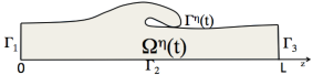
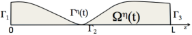
Figure 3: Two ways a fluid domain can degenerate. Left: loss of injectivity of the ALE mapping ${\bf A}_{\eta}$. Right: loss of injectivity of the ALE mapping ${\bf A}_{\eta}$ and loss strict positivity of the Jacobian $J^{\eta}$.

3.3 The weak ALE formulation

As mentioned earlier, we will prove the existence of a weak solution to problem (9)-(14) by mapping the problem defined on the moving domain $\Omega^{\eta}(t)$ onto a fixed, reference domain $\Omega$, and study the transformed problem on $\Omega$. For this purpose we map the functions defined on the moving domain $\Omega^{\eta}(t)$ onto the reference domain using the ALE mapping introduced above. We will use super-script $\eta$ to denote that those functions now depend (implicitly) on $\boldsymbol{\eta}$. More precisely, let ${\bf f}$ be a (scalar or vector) function defined on $\Omega^{\eta}(t)$. Then ${\bf f}^{\eta}$, defined on $\Omega$, is given by:

$${\bf f}^{\eta}(t,z,r)={\bf f}\big{(}t,{\bf A}_{\eta}(t)(z,r)\big{)}={\bf f}(t,x,y),$$

where $(x,y)={\bf A}_{\eta}(t)(z,r)\in\Omega^{\eta}(t)$ denotes the coordinates in $\Omega^{\eta}(t)$. Furthermore, we define the transformed gradient and divergence operators by

$$\nabla^{\eta}{\bf f}^{\eta}(t):=(\nabla{\bf f}(t))^{\eta}=\nabla{\bf f}^{\eta}(\nabla A_{\eta}(t))^{-1},\;\nabla^{\eta}\cdot{\bf f}^{\eta}={\rm tr}\big{(}\nabla^{\eta}{\bf f}^{\eta}\big{)}.$$ (33)

It will be useful in the remainder of the paper to obtain a relationship between the gradient $\nabla^{\eta}$ and symmetrized gradient ${\bf D}^{\eta(t,.)}$ of the fluid velocity ${\bf u}$ defined on $\Omega$. This is typically given via Korn’s inequality. However, the problem is that the fluid velocity ${\bf u}^{\eta}(t,z,r)$ for $t\in(0,T)$, which is defined on the fixed domain $\Omega$, is coming from a family of velocities ${\bf u}$ defined on domains $\Omega^{\eta}(t)$ for $t\in(0,T)$, via a family of ALE mappings, all depending on $\boldsymbol{\eta}$. We now show that if $\boldsymbol{\eta}$ is “nice enough”, there exists a uniform Korn’s constant, independent of the family of domains, such that a version of Korn’s inequality holds. More precisely, the following Lemma holds true.

Lemma 1.

(The “transformed” Korn’s inequality) Let

1. $\boldsymbol{\eta}\in L^{\infty}(0,T;H^{2}(\Gamma))\cap W^{1,\infty}(0,L;L^{2}(\Gamma))$, and

2. $\boldsymbol{\eta}(0,.)=\boldsymbol{\eta}_{0}$ where $\boldsymbol{\eta}_{0}$ satisfies conditions (16) and (17).

Then there exists a time $T^{\prime}>0$ and constants $C,c>0$ depending only on $\|\boldsymbol{\eta}\|_{L^{\infty}(H^{2})\cap W^{1,\infty}(L^{2})}$, such that for every ${\bf u}^{\eta}\in H^{1}(\Omega)^{2}$ satisfying boundary condition (13) on $\Sigma$, the following transformed version of Korn’s inequality holds:

$$c\|{\bf D}^{\eta(t,.)}({\bf u})\|_{L^{2}(\Omega)}\leq\|\nabla^{\eta(t,.)}({\bf u})\|_{L^{2}(\Omega)}\leq C\|{\bf D}^{\eta(t,.)}({\bf u})\|_{L^{2}(\Omega)},\;t\in[0,T^{\prime}].$$

The time $T^{\prime}>0$ is determined by the injectivity of the ALE mapping ${\bf A}_{\eta}$.

Proof.

From Proposition 1 we deduce the existence of a $T^{\prime}>0$ such that ${\bf A}_{\eta}(t)$ is injective for every $t\in[0,T^{\prime}]$. Now, the statement of the Lemma follows from the results in [56] (Lemma 1 and Remark 6) in the same way as in [42]. Namely, for each fixed $t\in(0,T^{\prime})$ we map ${\bf u}$ back to the physical domain $\Omega^{\eta}(t)$ and apply Korn’s inequality there in a standard way, using the classical Korn’s constant which depends on domain $\Omega^{\eta}(t)$ defined by $\boldsymbol{\eta}$. Due to the regularity of $\boldsymbol{\eta}$ given by conditions 1. and 2. in the statement of the Lemma, and due to the uniform (in $t$) estimate (25), it follows that the set $\{{\bf A}_{\eta}(t):t\in(0,T^{\prime})\}$ is compact in $W^{1,\infty}(\Omega)^{2}$, from which the existence of universal Korn constants $c$ and $C$ follows. ∎

To define the ALE formulation of problem (9)-(14) we recall the definition of the ALE velocity given in (26) and define the ALE derivative as a time derivative evaluated on the fixed reference domain:

$$\partial_{t}{\bf f}_{|\Omega}=\partial_{t}{\bf f}+({\bf w}^{\eta}\cdot\nabla){\bf f}.$$ (34)

Using the ALE mapping we can rewrite the Navier-Stokes equations in the ALE formulation as follows:

$$\partial_{t}{\bf u}_{|\Omega}+({\bf u}-{\bf w}^{\eta})\cdot\nabla{\bf u}=\nabla\cdot\boldsymbol{\sigma}\quad{\rm in}\;\Omega^{\eta}(t).$$ (35)

Here, the terms $\partial_{t}{\bf u}_{|\Omega}$ and ${\bf w}^{\eta}$, which are originally defined on $\Omega$, are composed with the inverse of the ALE mapping, which maps them back to the moving domain $\Omega^{\eta}(t)$.

Our goal is to define weak solutions to problem (9)-(14) on the fixed, reference domain $\Omega$. The first step is to introduce the necessary function spaces on $\Omega$. For this purpose we notice that the incompressibility condition in moving domains $\nabla\cdot{\bf u}=0$ transforms into the following condition on $\Omega$:

$$\nabla^{\eta}\cdot{\bf u}^{\eta}=0,$$

which we will call the transformed divergence-free condition.

Motivated by the energy inequality (18) we can now define the function spaces associated with weak solutions of problem (9)-(14). We define the analogue of the classical function space for the fluid velocity with the transformed divergence-free condition:

$${\mathcal{V}}_{F}^{\eta}=\{{\bf u}^{\eta}=(u_{z}^{\eta},u_{r}^{\eta})\in H^{1}(\Omega)^{2}:\nabla^{\eta}\cdot{\bf u}^{\eta}=0,{\bf u}^{\eta}\cdot\boldsymbol{\tau}^{\eta}=0,\;{\rm on}\ \Gamma_{i},\;i\in I,\;$$

$${\bf u}^{\eta}=0\ {\rm on}\ \Gamma_{i},\;i\in II,\;{\bf u}^{\eta}\cdot\boldsymbol{\nu}^{\eta}=0,\;{\rm on}\ \Gamma_{i},\;i\in III\cup IV\}.$$

The corresponding space involving time is given by:

$${\mathcal{W}}_{F}^{\eta}(0,T)=L^{\infty}(0,T;L^{2}(\Omega))\cap L^{2}(0,T;{\cal V}_{F}^{\eta}).$$ (36)

The structure function spaces are classical:

$${\mathcal{W}}_{S}(0,T)=W^{1,\infty}(0,T;L^{2}(0,L))^{2}\cap L^{\infty}(0,T;H^{2}_{0}(\Gamma))^{2}.$$ (37)

The solution space for our problem with the slip boundary condition must incorporate the continuity of normal velocities:

$${\mathcal{W}^{\eta}}(0,T)=\{({\bf u}^{\eta},\boldsymbol{\eta})\in{\cal W}_{F}^{\eta}(0,T)\times{\cal W}_{S}(0,T):{\bf u}^{\eta}_{|\Gamma}\cdot\boldsymbol{\nu}^{\eta}=\partial_{t}\boldsymbol{\eta}\cdot\boldsymbol{\nu}^{\eta}\}.$$ (38)

The corresponding test space is defined by

$${\mathcal{Q}^{\eta}}(0,T)=\{({\bf q}^{\eta},\boldsymbol{\psi})\in C^{1}_{c}([0,T);{\cal V}_{F}^{\eta}\times H_{0}^{2}(\Gamma)^{2}):{\bf q}^{\eta}_{|\Gamma}\cdot\boldsymbol{\nu}^{\eta}=\boldsymbol{\psi}(t,z)\cdot\boldsymbol{\nu}^{\eta}\}.$$ (39)

To obtain the weak formulation on $\Omega$ we first consider our problem defined on moving domains $\Omega^{\eta}(t)$. Take a test function ${\bf q}$ defined on $\Omega^{\eta}(t)$ for some $\boldsymbol{\eta}$, such that the corresponding test function ${\bf q}^{\eta}$ defined on the fixed domain belongs to the test space ${\mathcal{Q}^{\eta}}(0,T)$, namely, $({\bf q}^{\eta},\boldsymbol{\psi})\in{\mathcal{Q}^{\eta}}(0,T)$. Multiply (35) by ${\bf q}$, integrate over $\Omega^{\eta}(t)$, and formally integrate by parts. We obtain the following. For the convective term we have:

$$\int_{\Omega^{\eta}(t)}(({\bf u}-{\bf w}^{\eta})\cdot\nabla){\bf u}\cdot{\bf q}=\displaystyle{\frac{1}{2}\int_{\Omega^{\eta}(t)}(({\bf u}-{\bf w}^{\eta})\cdot\nabla){\bf u}\cdot{\bf q}-\frac{1}{2}\int_{\Omega^{\eta}(t)}(({\bf u}-{\bf w}^{\eta})\cdot\nabla){\bf q}\cdot{\bf u}}$$

$$\displaystyle{+\frac{1}{2}\int_{\Gamma^{\eta}(t)}({\bf u}-{\bf w}^{\eta})\cdot\boldsymbol{\nu}^{\eta}({\bf u}\cdot{\bf q})d\Gamma^{\eta}+\frac{1}{2}\int_{\Omega^{\eta}(t)}(\nabla\cdot{\bf w}^{\eta}){\bf u}\cdot{\bf q}-\frac{1}{2}\sum_{i\in I}\int_{\Gamma_{i}}|{\bf u}|^{2}q_{\nu}}.$$

For the diffusive part of the Navier-Stokes equations we have:

$$-\int_{\Omega^{\eta}(t)}(\nabla\cdot\boldsymbol{\sigma})\cdot{\bf q}=2\mu\int_{\Omega^{\eta}(t)}{\bf D}({\bf u}):{\bf D}({\bf q})-\int_{\partial\Omega^{\eta}(t)}\boldsymbol{\sigma}\boldsymbol{\nu}^{\eta}\cdot{\bf q},$$

where the second term on the right hand side can be expressed as follows:

$$\int_{\partial\Omega^{\eta}(t)}\boldsymbol{\sigma}\boldsymbol{\nu}^{\eta}\cdot{\bf q} =\int_{\Gamma^{\eta}(t)}\Big{(}(\boldsymbol{\sigma}\boldsymbol{\nu}^{\eta}\cdot\boldsymbol{\nu}^{\eta}){\bf q}\cdot\boldsymbol{\nu}^{\eta}+(\boldsymbol{\sigma}\boldsymbol{\nu}^{\eta}\cdot\boldsymbol{\tau}^{\eta}){\bf q}\cdot\boldsymbol{\tau}^{\eta}\Big{)}d\Gamma^{\eta}$$

$$+\sum_{i\in I}\int_{\Gamma_{i}}pq_{\nu}+\sum_{i\in III}\int_{\Gamma_{i}}(\boldsymbol{\sigma}\boldsymbol{\nu}\cdot\boldsymbol{\tau}){\bf q}\cdot\boldsymbol{\tau}$$

$$=\int_{\Gamma^{\eta}(t)}\Big{(}(\boldsymbol{\sigma}\boldsymbol{\nu}^{\eta}\cdot\boldsymbol{\nu}^{\eta})\boldsymbol{\psi}\cdot\boldsymbol{\nu}^{\eta}+\frac{1}{\alpha}(\partial_{t}\boldsymbol{\eta}-{\bf u})\cdot\boldsymbol{\tau}^{\eta}({\bf q}\cdot\boldsymbol{\tau}^{\eta})\Big{)}d\Gamma^{\eta}$$

$$+\sum_{i\in I}\int_{\Gamma_{i}}pq_{\nu}-\sum_{i\in III}\int_{\Gamma_{i}}\frac{1}{\alpha_{i}}u_{\tau}q_{\tau}.$$

We sum all the integrals, and take into account the coupling conditions (10)-(12) holding along $\Gamma^{\eta}(t)$, and boundary conditions (13) holding along $\Sigma$. To deal with the non-zero data on $\Gamma_{i},i\in I$ we introduce the “source term functional” ${\bf R}$ which will collect the two terms corresponding to dynamic pressure data defined on $\Gamma_{i},i\in I$:

$$\langle{\bf R},{\bf q}\rangle:=\sum_{i\in I}\int_{\Gamma_{i}}P_{i}{\bf q}\cdot{\boldsymbol{\nu}},\quad\forall{\bf q}\in C_{c}^{1}([0,T)\times\overline{\Omega}),$$ (40)

where $\boldsymbol{\nu}$ is the unit outward normal to the boundary $\Gamma_{i},i\in I$. Then we integrate the entire expression with respect to time over $(0,T)$ to obtain the following weak ALE formulation of problem (9)-(14) defined on $\Omega^{\eta}(t)$:

$$\begin{array}[]{c}\displaystyle{\rho_{F}\int_{0}^{T}\int_{\Omega^{\eta}(t)}\left(\partial_{t}{\bf u}^{\eta}_{|\Omega}\cdot{\bf q}+\frac{1}{2}\big{(}(({\bf u}-{\bf w}^{\eta})\cdot\nabla){\bf u}\cdot{\bf q}-(({\bf u}-{\bf w}^{\eta})\cdot\nabla){\bf q}\cdot{\bf u}\big{)}+\frac{1}{2}(\nabla\cdot{\bf w}^{\eta}){\bf u}\cdot{\bf q}\right)}\\ \displaystyle{+\int_{0}^{T}\left\{2\mu\int_{\Omega^{\eta}(t)}{\bf D}({\bf u}):{\bf D}({\bf q})+\sum_{i\in III}\int_{\Gamma_{i}}\frac{1}{\alpha_{i}}u_{\tau}q_{\tau}+\frac{1}{\alpha}\int_{\Gamma^{\eta}(t)}(u_{\tau^{\eta}}-\partial_{t}\eta_{\tau^{\eta}})q_{\tau^{\eta}}d\Gamma^{\eta}(t)\right\}dt}\\ \displaystyle{+\rho_{S}h\int_{0}^{T}\int_{\Gamma}\partial^{2}_{t}\boldsymbol{\eta}\boldsymbol{\psi}dzdt}\displaystyle{+\int_{0}^{T}\langle{\mathcal{L}}_{e}\boldsymbol{\eta},\boldsymbol{\psi}\rangle dt+\frac{1}{\alpha}\int_{0}^{T}\int_{\Gamma}(\partial_{t}\eta_{\tau^{\eta}}-u_{\tau^{\eta}})\phi_{\tau^{\eta}}S^{\eta}dzdt=\int_{0}^{T}\langle{\bf R},{\bf q}\rangle},\end{array}$$ (41)

for all $({\bf q},\boldsymbol{\psi})$ such that $({\bf q}^{\eta},\boldsymbol{\psi})\in{\mathcal{Q}}^{\eta}(0,T)$, where $g_{\tau^{\eta}}={\bf q}\cdot\boldsymbol{\tau}^{\eta}$ and $g_{\nu^{\eta}}={\bf q}\cdot\boldsymbol{\nu}^{\eta}$ denotes the tangential and normal component of ${\bf q}$, respectively, and the source term functional ${\bf R}$ is defined in (40) to account for the non-zero dynamic pressure boundary condition on $\Gamma_{i},i\in I$.

We now transform (41) to the fixed reference domain via the ALE mapping ${\bf A}_{\eta}$. To do that we first compute the integral involving the ALE derivative $\partial_{t}{\bf u}^{\eta}_{|\Omega}$:

$$\int_{0}^{T}\int_{\Omega^{\eta}(t)}\partial_{t}{\bf u}^{\eta}_{|\Omega}\cdot{\bf q} =\int_{0}^{T}\int_{\Omega}J^{\eta}\partial_{t}{\bf u}^{\eta}\cdot{\bf q}^{\eta}$$

$$= -\int_{0}^{T}\int_{\Omega}\partial_{t}J^{\eta}{\bf u}^{\eta}\cdot{\bf q}^{\eta}-\int_{0}^{T}\int_{\Omega}J^{\eta}{\bf u}^{\eta}\cdot\partial_{t}{\bf q}^{\eta}-\int_{\Omega}J_{0}{\bf u}_{0}\cdot{\bf q}^{\eta}(0,.).$$

Now, since

$$\partial_{t}J^{\eta}=J^{\eta}\nabla^{\eta}\cdot{\bf w}^{\eta}$$ (42)

(see e.g. [25], p. 77), the above expression reads

$$\int_{0}^{T}\int_{\Omega^{\eta}(t)}\partial_{t}{\bf u}^{\eta}_{|\Omega}\cdot{\bf q}=-\int_{0}^{T}\int_{\Omega}\left\{J^{\eta}\left(\nabla^{\eta}\cdot{\bf w}^{\eta}\right)\left({\bf u}^{\eta}\cdot{\bf q}^{\eta}\right)-J^{\eta}{\bf u}^{\eta}\cdot\partial_{t}{\bf q}^{\eta}\right\}-\int_{\Omega}J_{0}{\bf u}_{0}\cdot{\bf q}^{\eta}(0,.).$$

Now, we can define the weak solution on the fixed reference domain.

NOTATION. To simplify notation, from this point on we will omit the superscript $\eta$ in ${\bf u}^{\eta}$ and ${\bf q}^{\eta}$ since everything will be happening only on the fixed, reference domain, and there will be no place for confusion.

Definition 1.

(Weak solution) We say that $({\bf u},\boldsymbol{\eta})\in{\mathcal{W}}^{\eta}(0,T)$ is a weak solution to problem (9)-(14) defined on the reference domain $\Omega$, if for every $({\bf q},\boldsymbol{\psi})\in{\mathcal{Q}}^{\eta}(0,T)$ the following equality holds:

$$\begin{array}[]{c}\displaystyle{\frac{\rho_{F}}{2}\int_{0}^{T}\int_{\Omega}J^{\eta}\Big{(}(({\bf u}-{\bf w}^{\eta})\cdot\nabla^{\eta}){\bf u}\cdot{\bf q}-(({\bf u}-{\bf w}^{\eta})\cdot\nabla^{\eta}){\bf q}\cdot{\bf u}}-(\nabla^{\eta}\cdot{\bf w}^{\eta}){\bf q}\cdot{\bf u}\Big{)}\\ \\ \displaystyle{-\rho_{F}\int_{0}^{T}\int_{\Omega}J^{\eta}{\bf u}\cdot\partial_{t}{\bf q}+\int_{0}^{T}2\mu\int_{\Omega}J^{\eta}{\bf D}^{\eta}({\bf u}):{\bf D}^{\eta}({\bf q})+\sum_{i\in III}\int_{0}^{T}\int_{\Gamma_{i}}\frac{1}{\alpha_{i}}u_{\tau}q_{\tau}}\\ \\ \displaystyle{+\frac{1}{\alpha}\int_{0}^{T}\int_{\Gamma}(u_{\tau^{\eta}}-\partial_{t}\eta_{\tau^{\eta}})q_{\tau^{\eta}}S^{\eta}dzdt-\rho_{S}h\int_{0}^{T}\int_{\Gamma}\partial_{t}\boldsymbol{\eta}\partial_{t}\boldsymbol{\psi}dzdt+\int_{0}^{T}\langle{\mathcal{L}}_{e}\boldsymbol{\eta},\boldsymbol{\psi}\rangle}\\ \\ \displaystyle{+\frac{1}{\alpha}\int_{0}^{T}\int_{\Gamma}(\partial_{t}\eta_{\tau^{\eta}}-u_{\tau^{\eta}})\psi_{\tau^{\eta}}S^{\eta}dzdt=\int_{0}^{T}\langle{\bf R},{\bf q}\rangle+\int_{\Omega}J_{0}{\bf u}_{0}\cdot{\bf q}(0)+\int_{\Gamma}{\bf v}_{0}\cdot\boldsymbol{\psi}},\end{array}$$ (43)

where $J^{\eta}$ is the determinant of the Jacobian of ALE mapping, defined in (29), and ${\bf w}^{\eta}$ is the ALE velocity, defined in (26).

We note that Definition 1 makes sense even in the case when the ALE mapping ${\bf A}_{\eta}$ is not injective. However, in that case the weak formulation (43) is not equivalent to problem (9)-(14) even for smooth solutions.

4 Main Result

We are now in a position to state the main result of this work. For this purpose we shall assume that all the moving domains $\Omega^{\eta}(t)$ are contained in a larger domain $\Omega_{\rm max}$. Indeed, it will be shown later, see Corollary 2, that this will be the case. We note that the only reason for this assumption is to assume a certain regularity of the source term ${\bf R}$, associated with the non-zero boundary data on $\Sigma$. Namely, we will be assuming that ${\bf R}\in L^{2}(0,T;H^{1}(\Omega_{\rm max})^{\prime})$, where $(H^{1})^{\prime}$ denotes the dual space of $H^{1}$. In the case when only the dynamic pressure boundary data is different from zero, the introduction of the source term ${\bf R}$ is not necessary. However, we state the Main Result in general terms, and consider $\Omega_{\rm max}$ to be the union of all the moving domains $\Omega^{\eta}(t)$.

Theorem 2.

(Main result) Let all the parameters in the problem be positive (this includes the fluid and structure densities $\rho_{F}$ and $\rho_{S}$, structure thickness $h$, and the slip-condition friction constants $\alpha$ on the moving boundary $\Gamma^{\eta}(t)$, and $\alpha_{i}$’s on the rigid boundary $\Gamma_{III}$). Moreover, let the source term functional ${\bf R}$, defined in (40), be such that ${\bf R}\in L^{2}(0,\infty;H^{1}(\Omega_{\rm max})^{\prime})$. If the initial data ${\bf u}_{0}\in L^{2}(\Omega^{0})$ and $\boldsymbol{\eta}_{0}\in H^{2}_{0}(\Gamma)$ are such that compatibility conditions (15), (16) and (17) are satisfied, then there exists a $T>0$ and a weak solution $({\bf u},\boldsymbol{\eta})$ to problem (9)-(14) defined on $(0,T)$, such that the following energy estimate is satisfied:

$$\begin{array}[]{c}\displaystyle{\frac{1}{2}\big{(}\rho_{F}\|{\bf u}\|^{2}_{L^{\infty}(0,T;L^{2}(\Omega^{\eta}(t))}+\rho_{S}h\|\partial_{t}\boldsymbol{\eta}\|^{2}_{L^{\infty}(0,T;L^{2}(\Gamma))}+c\|\boldsymbol{\eta}\|^{2}_{L^{\infty}(0,T;H^{2}(\Gamma))}\big{)}+\mu\|{\bf D}({\bf u})\|^{2}_{L^{2}(0,T;L^{2}(\Omega^{\eta}(t)))}}\\ \\ \displaystyle{+\frac{1}{\alpha}\|u_{\tau}-\partial_{t}\eta_{\tau}\|^{2}_{L^{2}(0,T;L^{2}(\Gamma^{\eta}(t)))}+\sum_{i\in III}\frac{1}{\alpha_{i}}\|u_{\tau}\|^{2}_{L^{2}(0,T;L^{2}(\Gamma_{i}))}\leq E_{0}+C\|{\bf R}\|^{2}_{L^{2}(0,T;H^{1}(\Omega^{\eta}(t))^{\prime})},}\end{array}$$ (44)

where $C$ depends only on the initial data and on the parameters in the problem, and $E_{0}$ is the kinetic and elastic energy of the initial data.

The proof of this theorem is based on the following approach. We design a partitioned time-marching scheme by using the time-discretization via Lie operator spitting. We first separate the fluid and structure subproblems and then semi-discretize the resulting sub-problems with respect to time. The time interval $(0,T)$ is subdivided into $N$ sub-intervals $(0,t_{1}),\cdots,(t_{N-1},t_{N})$ each of width $\Delta t$, and the fluid and structure sub-problems are solved on each sub-interval. First, the structure sub-problem is solved on $(t_{i-1},t_{i})$ using for the initial data the solution of the fluid sub-problem from the previous time step, and then the fluid sub-problem is solved on $(t_{i-1},t_{i})$ using for the initial data the solution of the just calculated structure sub-problem. The process is repeated for each sub-interval of $(0,T)$. This defines an approximation of the solution of the coupled FSI problem on $(0,T)$. On each sub-interval $(t_{i-1},t_{i})$ the transfer of information between the two sub-problems is achieved via the “initial data” at $t_{i-1}$. At each time step only one iteration for the fluid sub-problem and one for the structure sub-problem are sufficient to obtain a stable and convergent algorithm. The goal is to show that as the time-discretization step $\Delta t\to 0$, the sequence of approximate solutions, described above, converges to a weak solution of the coupled FSI problem.

A crucial step in this approach is the way how the fluid and structure sub-problems are designed. In particular, we had to be careful to take into account the well-known problems related to the so called “added mass effect” [9] to design the fluid sub-problem in such a way that the fluid and structure inertia are kept close together via a Robin-type boundary condition for the fluid sub-problem. In contrast with the no-slip boundary condition, the slip boundary condition is more tricky to deal with because of the lack of continuity in the tangential component of the velocity at the fluid-structure interface, and so the smoothing of the interface due to the viscous fluid dissipation is no longer transferred to the structure in the tangential direction. New compactness arguments based on the theorem of Simon [53] and on interpolation of classical Sobolev spaces with real exponents $H^{s}$ (or alternatively Nikolskii spaces) will be used to obtain the existence result. Details are presented next.

5 Approximate solutions

We construct approximate solutions to problem (9)-(14) by using the time-discretization via Lie operator splitting.

5.1 Operator splitting scheme

Let ${\Delta t}=T/N$ be the time-discretization parameter so that the time interval $(0,T)$ is sub-divided into $N$ sub-intervals of width $\Delta t$. On each sub-interval we split the problem into a fluid and structure sub-problem, and linearize each sub-problem appropriately. Each of the sub-problems will be discretized in time using the Backward Euler scheme.

To perform the Lie splitting we must rewrite problem (9)-(14) as a first-order system in time

$$\frac{d{\bf X}}{dt} =A{\bf X},\ t\in(0,T),$$

$${\bf X}|_{t=0} ={\bf X}^{0},$$ (45)

where $A$ is an operator on a Hilbert space, such that $A$ can be split into a non-trivial decomposition $A=A_{1}+A_{2}$. For this purpose introduce the substitution ${\bf v}=\partial_{t}\boldsymbol{\eta}$, and rewrite the structure acceleration in terms of the first-order derivative of structure velocity. The initial approximation of the solution will be the initial data in the problem, namely, ${\bf u}^{0}={\bf u}_{0}$, $\boldsymbol{\eta}^{0}=\boldsymbol{\eta}_{0}$, and ${\bf v}^{0}={\bf v}_{0}$. For every sub-division of $(0,T)$ containing $N\in{\mathbb{N}}$ sub-intervals, we recursively define the vector of unknown approximate solutions

$${\bf X}_{\Delta t}^{n+\frac{i}{2}}=\left(\begin{array}[]{c}{\bf u}_{\Delta t}^{n+\frac{i}{2}}\\ {\bf v}_{\Delta t}^{n+\frac{i}{2}}\\ \boldsymbol{\eta}_{\Delta t}^{n+\frac{i}{2}}\end{array}\right),n=0,1,\dots,N-1,\,\ i=1,2,$$ (46)

where $i=1,2$ denotes the solution of sub-problems defined by $A_{1}$ or $A_{2}$, respectively. The initial condition is given by the initial data in the problem. ${\bf X}^{0}=({\bf u}_{0},{\bf v}_{0},\boldsymbol{\eta}_{0})^{T}.$

A crucial ingredient for the existence proof is that the semi-discretization of the split problem be performed in such a way that a semi-discrete version of the energy inequality (44) is preserved at every time step. This is associated with successfully dealing with the “added mass effect” [9, 42]. For this purpose we define a semi-discrete version of the total energy and dissipation at time $n\Delta t$ as follows:

$$E^{n+i/2}_{\Delta t}=\frac{\rho_{F}}{2}\int_{\Omega}J^{n}|{\bf u}^{n}_{\Delta t}|^{2}+\frac{\rho_{S}h}{2}\big{(}\|{\bf v}^{n+i/2}_{\Delta t}\|^{2}_{L^{2}(\Gamma)}+\langle{\mathcal{L}}_{e}\boldsymbol{\eta}^{n+i/2}_{\Delta t},\boldsymbol{\eta}^{n+i/2}_{\Delta t}\rangle\big{)},\;i=0,1;$$ (47)

$$D^{n}_{\Delta t}={\Delta t}\mu\int_{\Omega}J^{n}{\bf D}({\bf u}^{n}_{\Delta t}):{\bf D}({\bf u}^{n}_{\Delta t})+\frac{\Delta t}{2}\sum_{i\in III}\int_{\Gamma_{i}}\frac{1}{\alpha_{i}}({u^{n}_{\Delta t}})_{\tau}({u^{n}_{\Delta t}})_{\tau}+\frac{\Delta t}{\alpha}\|(v^{n}_{\Delta t})_{\tau}-(u^{n}_{\Delta t})_{\tau}\|^{2}_{L^{2}(\Gamma)}.\;$$ (48)

Throughout the rest of this section, we keep the time step $\Delta t$ fixed, and define the semi-discretized fluid and structure sub-problems. To simplify notation, we will omit the subscript $\Delta t$ and write $({\bf u}^{n+\frac{i}{2}},{\bf v}^{n+\frac{i}{2}},\boldsymbol{\eta}^{n+\frac{i}{2}})$ instead of $({\bf u}^{n+\frac{i}{2}}_{\Delta t},{\bf v}^{n+\frac{i}{2}}_{\Delta t},\boldsymbol{\eta}^{n+\frac{i}{2}}_{\Delta t})$.

THE STRUCTURE SUB-PROBLEM (Differential formulation):

$$\left.\begin{array}[]{c}\displaystyle{\rho_{S}h\frac{{\bf v}^{n+1/2}-{\bf v}^{n}}{\Delta t}+{\mathcal{L}}_{e}\boldsymbol{\eta}^{n+1}=0,}\\ \\ \displaystyle{\frac{\boldsymbol{\eta}^{n+1}-\boldsymbol{\eta}^{n}}{\Delta t}={\bf v}^{n+1/2},}\end{array}\right\}\;{\rm on}\;\Gamma,$$ (49)

$$\boldsymbol{\eta}^{n+1}(0)=\partial_{z}\boldsymbol{\eta}^{n+1}(0)=\boldsymbol{\eta}^{n+1}(L)=\partial_{z}\boldsymbol{\eta}^{n+1}(L)=0.$$

The weak formulation is given by: find $({\bf v}^{n+1/2},\boldsymbol{\eta}^{n+1})\in H^{2}_{0}(\Gamma)^{4}$ such that

$$\begin{array}[]{c}\displaystyle{\rho_{S}h\int_{\Gamma}\frac{{\bf v}^{n+1/2}-{\bf v}^{n}}{\Delta t}\cdot\boldsymbol{\psi}+\langle{\mathcal{L}}_{e}\boldsymbol{\eta}^{n+1},\boldsymbol{\psi}\rangle=0,\quad\boldsymbol{\psi}\in[H^{2}_{0}(\Gamma)]^{2},}\\ \displaystyle{\int_{\Gamma}\frac{\boldsymbol{\eta}^{n+1}-\boldsymbol{\eta}^{n}}{\Delta t}\cdot{\boldsymbol{\varphi}}=\int_{\Gamma}{\bf v}^{n+1/2}\cdot\boldsymbol{\varphi},}\quad\boldsymbol{\varphi}\in[L^{2}(\Gamma)]^{2}.\end{array}$$ (50)

This problem is similar to the structure sub-problem for the fluid-structure interaction problem studied in [42], where the no-slip boundary condition was considered, and only the radial displacement of the thin structure was assumed to be different from zero. Using the same ideas as in [42] one can show that the following existence result and energy estimate hold for problem (50):

Proposition 2.

For each fixed $\Delta t>0$, problem (50) has a unique solution $({\bf v}^{n+\frac{1}{2}},\boldsymbol{\eta}^{n+\frac{1}{2}})\in[H^{2}_{0}(\Gamma)]^{2}\times[H_{0}^{2}(\Gamma)]^{2}$. Moreover, the solution of problem (50) satisfies the following discrete energy inequality:

$$\begin{array}[]{c}\displaystyle{E_{\Delta t}^{n+\frac{1}{2}}+\frac{1}{2}\big{(}\rho_{s}h\|{\bf v}^{n+\frac{1}{2}}-{\bf v}^{n}\|^{2}+c\|\boldsymbol{\eta}^{n+\frac{1}{2}}-\boldsymbol{\eta}^{n}\|^{2}_{H^{2}_{0}}\big{)}\leq E_{\Delta t}^{n},}\end{array}$$ (51)

where the kinetic energy $E_{\Delta t}^{n}$ is defined in (47), and $c$ is the coercivity constant defined in (4).

Proof.

The proof of this proposition is similar to the proof in Propositions 1 and 2 in [42]. The existence of a unique weak solution follows from the Lax-Milgram Lemma as in [42].

The energy inequality is obtained by using ${\bf v}^{n+1/2}$ in place of the structure velocity test function $\boldsymbol{\psi}$ in the first term in the first equation in (50), and by using $\frac{\boldsymbol{\eta}^{n+1/2}-\boldsymbol{\eta}^{n}}{\Delta t}$ in place of the structure velocity test function $\boldsymbol{\psi}$ in the second term in the first equation in (50). After a calculation incorporating the equality $|(a-b)a|=\frac{1}{2}(|a|^{2}+|a-b|^{2}-|b|^{2})$, one gets

$$\frac{\rho_{S}h}{2}\|{\bf v}^{n+1/2}\|^{2}_{L^{2}}+\frac{\rho_{S}h}{2}\|{\bf v}^{n+1/2}-{\bf v}^{n}\|^{2}_{L^{2}}+ \frac{1}{2}\langle{\cal{L}}_{e}\boldsymbol{\eta}^{n+1/2},\boldsymbol{\eta}^{n+1/2}\rangle+\frac{1}{2}\langle{\cal{L}}_{e}(\boldsymbol{\eta}^{n+1/2}-\boldsymbol{\eta}^{n}),(\boldsymbol{\eta}^{n+1/2}-\boldsymbol{\eta}^{n})\rangle$$

$$=\frac{\rho_{S}h}{2}\|{\bf v}^{n}\|^{2}_{L^{2}}+\frac{1}{2}\langle{\cal{L}}_{e}\boldsymbol{\eta}^{n},\boldsymbol{\eta}^{n}\rangle.$$

We add the term $\frac{\rho_{f}}{2}\int_{\Omega}J^{n}|{\bf u}_{\Delta t}^{n}|^{2}$ on both sides of the above equality, and use the coercivity property of ${\cal{L}}_{e}$ to obtain the energy inequality (51). ∎

Remark. We would like to draw the attention of the reader to the fact that the estimate of the term $\|\boldsymbol{\eta}^{n+\frac{1}{2}}-\boldsymbol{\eta}^{n}\|^{2}_{H^{2}_{0}}$ was made possible by the fact that we are performing the time-discretization via operator splitting, and study semi-discretized problems in time. As a result, the approximation of the structure velocity, which was semi-disretized using the backward Euler method, gives rise to the term $\|\boldsymbol{\eta}^{n+\frac{1}{2}}-\boldsymbol{\eta}^{n}\|^{2}_{H^{2}_{0}}$, which corresponds to the well-known numerical dissipation term. By the iterative application of inequality (51), the sum with respect to $n$ of the differences $\|\boldsymbol{\eta}^{n+\frac{1}{2}}-\boldsymbol{\eta}^{n}\|^{2}_{H^{2}_{0}}$ is uniformly bounded by a constant, which only depends on the initial kinetic energy and the inlet and outlet boundary data, as stated in Proposition 4 below. This estimate gives additional information about the behavior in time of the structure displacement, which will be crucial for the compactness arguments established in Section 6.2.

The structure sub-problem updates the position of the elastic boundary $\boldsymbol{\eta}^{n+1}$, based on which we can now calculate the ALE mapping ${\bf A}^{n+1}$ as the harmonic extension of $\boldsymbol{\eta}^{n+1}$, i.e. ${\bf A}^{n+1}={\bf id}+{\bf B}^{n+1}$ where ${\bf B}^{n+1}$ is defined as the solution of the following boundary value problem:

$${\Delta{\bf B}^{n+1}=0\;{\rm in}\;\Omega,\;{\bf B}^{n+1}_{|\Gamma}=\boldsymbol{\eta}^{n+1},\;{\bf B}^{n+1}_{|\Sigma}=0.}$$ (52)

The corresponding discrete version of the ALE velocity and the Jacobian of the ALE mapping are defined by:

$${\bf w}^{n+1}=\frac{{\bf A}^{n+1}-{\bf A}^{n}}{\Delta t},\;J^{n+1}=\det\nabla{\bf A}^{n+1}.$$ (53)

THE FLUID SUB-PROBLEM (Differential formulation):

$$\left.\begin{array}[]{rcl}\rho_{F}\displaystyle{\frac{{\bf u}^{n+1}-{\bf u}^{n}}{\Delta t}+\rho_{F}(({\bf u}^{n}-{\bf w}^{n+1})\cdot\nabla^{\eta^{n+1}}){\bf u}^{n+1}}&=&\displaystyle{\nabla^{\eta^{n+1}}\cdot\boldsymbol{\sigma}^{\eta^{n+1}}({\bf u}^{n+1},p^{n+1})}+{\bf R}^{n+1}\\ {\rm where}\ \displaystyle{{\bf R}^{n+1}}&=&\displaystyle{\frac{1}{\Delta t}\int_{n\Delta t}^{(n+1)\Delta t}{\bf R}}\end{array}\right\}\quad{\rm in}\ \Omega$$ (54)

$$\left.\begin{array}[]{rcl}\displaystyle{\frac{{\bf v}^{n+1}-{\bf v}^{n+1/2}}{\Delta t}}&=&\displaystyle{-S^{\eta^{n+1}}\boldsymbol{\sigma}^{\eta^{n+1}}({\bf u}^{n+1},p^{n+1})\boldsymbol{\nu}^{\eta^{n+1}}}\\ \displaystyle{({\bf u}^{n+1}-{\bf v}^{n+1})\cdot\boldsymbol{\nu}^{\eta^{n+1}}}&=&\displaystyle{0}\\ \displaystyle{\alpha\boldsymbol{\sigma}^{\eta^{n+1}}({\bf u}^{n+1},p^{n+1})\boldsymbol{\nu}^{\eta^{n+1}}\cdot\boldsymbol{\tau}^{\eta^{n+1}}}&=&\displaystyle{({\bf v}^{n+1}-\textbf{u}^{n+1})\cdot\boldsymbol{\tau}^{\eta^{n+1}}}\end{array}\right\}\quad{\rm on}\;\Gamma,$$ (55)

This system is supplemented with boundary conditions (13).

Before we state the corresponding weak formulation, we introduce the following abbreviations to simplify notation:

$$\nabla^{n}:=\nabla^{\eta^{n}},\;\boldsymbol{\sigma}^{n}:=\boldsymbol{\sigma}^{\eta^{n}},\;\boldsymbol{\nu}^{n}:=\boldsymbol{\nu}^{\eta^{n}},\;\boldsymbol{\tau}^{n}:=\boldsymbol{\tau}^{\eta^{n}},\;u^{n}_{\nu}:={\bf u}^{n}\cdot\boldsymbol{\nu}^{n},\;u^{n}_{\tau}:={\bf u}^{n}\cdot\boldsymbol{\tau}^{n}.$$ (56)

We now define the weak solution function space for the fluid sub-problem given in terms of the fluid velocity ${\bf u}$ and its trace ${\bf v}$ on $\Gamma$ as:

$${\mathcal{V}}^{n}=\{({\bf u},{\bf v})\in H^{1}(\Omega)^{2}\times L^{2}(\Gamma)^{2}:\nabla^{n}\cdot{\bf u}=0,\;({\bf u}-{\bf v})\cdot\boldsymbol{\nu}^{n}=0,$$

$${\bf u}\cdot\boldsymbol{\tau}=0,\;{\rm on}\ \Gamma_{i},\;i\in I,\;{\bf u}=0\ {\rm on}\ \Gamma_{i},\;i\in II,\;{\bf u}\cdot\boldsymbol{\nu}=0,\;{\rm on}\ \Gamma_{i},\;i\in III\cup IV\}.$$

The weak formulation is defined as follows: find $({\bf u}^{n+1},{\bf v}^{n+1})\in{\mathcal{V}}^{n}$ such that

$$\begin{array}[]{c}\displaystyle{\rho_{F}\int_{\Omega}J^{n}\frac{{\bf u}^{n+1}-{\bf u}^{n}}{\Delta t}\cdot{\bf q}+\frac{\rho_{F}}{2}\int_{\Omega}\frac{J^{n+1}-J^{n}}{\Delta t}{\bf u}^{n+1}\cdot{\bf q}+\frac{\rho_{F}}{2}\int_{\Omega}J^{n+1}\Big{(}(({\bf u}^{n}-{\bf w}^{n+1})\cdot\nabla^{n+1}){\bf u}^{n+1}\cdot{\bf q}}\\ \\ \displaystyle{-(({\bf u}^{n}-{\bf w}^{n+1})\cdot\nabla^{n+1}){\bf q}\cdot{\bf u}^{n+1}\Big{)}+2\mu\int_{\Omega}J^{n+1}{\bf D}({\bf u}^{n+1}):{\bf D}({\bf q})+\sum_{i\in III}\int_{\Gamma_{i}}\frac{1}{\alpha_{i}}{u}^{n+1}_{\tau}q_{\tau}}\\ \\ \displaystyle{+\frac{1}{\alpha}\int_{\Gamma}(u_{\tau}^{n+1}-v_{\tau}^{n+1})q_{\tau^{n+1}}S^{n+1}dz}\displaystyle{+\rho_{S}h\int_{\Gamma}\frac{{\bf v}^{n+1}-{\bf v}^{n+1/2}}{\Delta t}\boldsymbol{\psi}+\frac{1}{\alpha}\int_{\Gamma}({v}^{n+1}_{\tau}-u^{n+1}_{\tau})\psi_{\tau^{n+1}}S^{n+1}dz}\\ \\ \displaystyle{=\langle{\bf R}^{n+1},{\bf q}\rangle,\quad({\bf q},\boldsymbol{\psi})\in{\mathcal{V}}^{n}.}\end{array}$$ (57)

This is obtained by considering (43) and by using formula (42) to express $J^{\eta}(\nabla^{\eta}\cdot{\bf w}^{\eta})=\partial_{t}J^{\eta}$. Furthermore, in the third and fourth integral we replaced $J^{n}$ with $J^{n+1}$ for higher accuracy. This, however, does not influence the existence proof. Either choice works well.

Proposition 3.

Let $\Delta t>0$, and $J^{n+1}\geq c>0$. Then there exists a unique solution $({\bf u}^{n+1},{\bf v}^{n+1})$ to the fluid sub-problem (57). Furthermore, the solution satisfies the following semi-discrete energy inequality:

$$\begin{array}[]{c}\displaystyle{E^{n+1}_{\Delta t}+\frac{\rho_{F}}{2}\int_{\Omega}J^{n}\|{\bf u}^{n+1}-{\bf u}^{n}\|^{2}_{L^{2}(\Omega)}+\frac{\rho_{S}h}{2}\|{\bf v}^{n+1}-{\bf v}^{n+1/2}\|^{2}_{L^{2}(\Gamma)}}\\ \\ \displaystyle{+D^{n+1}_{\Delta t}\leq E^{n+1/2}_{\Delta t}+C\Delta t\|{\bf R}^{n+1}\|^{2}_{(H^{1}(\Omega))^{\prime}},}\end{array}$$ (58)

where $(H^{1}(\Omega))^{\prime}$ is the dual space of $H^{1}(\Omega)$.

Proof.

The existence proof follows from the Lax-Milgram Lemma and the transformed Korn’s inequality stated in Lemma 1, see [42].

The semi-discrete energy inequality (58) is a consequence of the fact that we have discretized our fluid sub-problem given by (57) so that the discrete version of the geometric conservation law is satisfied. More precisely, by taking ${\bf q}={\bf u}^{n+1}$ in the following two terms in the weak formulation (57):

$$\rho_{F}\int_{\Omega}J^{n}\frac{{\bf u}^{n+1}-{\bf u}^{n}}{\Delta t}\cdot{\bf q}+\frac{\rho_{F}}{2}\int_{\Omega}\frac{J^{n+1}-J^{n}}{\Delta t}{\bf u}^{n+1}\cdot{\bf q}$$

we see that with this kind of discretization a semi-discrete version of the geometric conservation law is exactly satisfied, i.e. we have:

$$\frac{\rho_{F}}{2}\Big{(}\int_{\Omega}J^{n+1}|{\bf u}^{n+1}|^{2}+\int_{\Omega}J^{n}|{\bf u}^{n+1}-{\bf u}^{n}|^{2}\Big{)}=\frac{\rho_{F}}{2}\int_{\Omega}J^{n}|{\bf u}^{n}|^{2}.$$ (59)

Thus, the fluid kinetic energy at time $(n+1)\Delta t$ plus the kinetic energy due to the fluid domain motion, is exactly equal to the fluid kinetic energy at time $n\Delta t$. The two terms on the left hand-side in (59) appear on the left hand-side in the energy estimate (58), while the term on the right hand-side in (59) appears on the right hand-side in the energy estimate (58). ∎

Proposition 4.

(Uniform semi-discrete energy estimates) Let $\Delta t>0$ and $N=T/\Delta t>0$. Furthermore, let $E_{\Delta t}^{n+\frac{1}{2}},E_{\Delta t}^{n+1}$, and $D_{\Delta t}^{n}$ be the kinetic energy and dissipation given by (47) and (48), respectively. There exists a constant $C>0$ independent of $\Delta t$, which depends only on the parameters in the problem, on the kinetic energy of the initial data $E_{0}$, and on the norm of the right-hand side $\|{\bf R}\|_{L^{2}(0,T;H^{1}(\Omega)^{\prime})}^{2}$ (i.e. on the boundary data), such that the following estimates hold: 1. $\displaystyle{E_{\Delta t}^{n+\frac{1}{2}}\leq C,E_{\Delta t}^{n+1}\leq C}$, for all $n=0,...,N-1,$
2. $\displaystyle{\sum_{n=1}^{N}D_{\Delta t}^{n}\leq C},$
3. $\displaystyle{\sum_{n=0}^{N-1}\Big{(}\int_{\Omega}J^{n}_{\Delta t}}|{\bf u}_{\Delta t}^{n+1}-{\bf u}_{\Delta t}^{n}|^{2}+\|{\bf v}_{\Delta t}^{n+1}-{\bf v}_{\Delta t}^{n+\frac{1}{2}}\|^{2}_{L^{2}(\Gamma)}+c\|\boldsymbol{\eta}_{\Delta t}^{n+1}-\boldsymbol{\eta}_{\Delta t}^{n}\|^{2}_{H^{2}(\Gamma)}+\|{\bf v}_{\Delta t}^{n+\frac{1}{2}}-{\bf v}_{\Delta t}^{n}\|^{2}_{L^{2}(\Gamma)}\Big{)}\leq C.$ In fact, $C=E_{0}+\tilde{C}\|{\bf R}\|^{2}_{L^{2}(0,T;H^{1}(\Omega)^{\prime})}$, where $\tilde{C}$ is a constant which depends only on the parameters in the problem, and ${\bf R}$ is the term, defined in (40), coming from the dynamic pressure data.

Proof.

The proof of Proposition 4 follows directly from the energy estimates (51) and (58), and from the Hölder inequality applied to the source term ${\bf R}$. More precisely, the statements in Proposition 4 are obtained after summing the combined energy estimates (51) and (58) over $n=0,\cdots,N-1$, and after taking into account that

$$\Delta t\sum_{n=0}^{N-1}\|{\bf R}^{n+1}\|^{2}_{(H^{1}(\Omega))^{\prime}}=\Delta t\sum_{n=0}^{N-1}\|\frac{1}{\Delta t}\int_{n\Delta t}^{{n+1}\Delta t}{\bf R}\|^{2}\leq\tilde{C}\|{\bf R}\|^{2}_{L^{2}(0,T;(H^{1}(\Omega))^{\prime})}.$$

∎

This is a crucial estimate which will provide uniform boundedness of approximating solutions to problem (9)-(14), constructed using our semi-discretized scheme based on Lie splitting. However, notice that we have so far only defined the approximate values of our solution at discrete points in time, given by $n\Delta t$. We want to define approximate solutions to be defined at all the points in $(0,T)$. For this purpose we define approximate solutions to be the functions which are piece-wise constant on each sub-interval $((n-1)\Delta t,n\Delta t],\ n=1\dots$ of $(0,T)$, such that for $t\in((n-1)\Delta t,n\Delta t],\ n=1\dots N,$

$${\bf u}_{\Delta t}(t,.)={\bf u}_{\Delta t}^{n},\ \eta_{\Delta t}(t,.)=\eta_{\Delta t}^{n},\ {\bf v}_{\Delta t}(t,.)={\bf v}_{\Delta t}^{n},\ v^{*}_{\Delta t}(t,.)={\bf v}^{n-\frac{1}{2}}_{\Delta t}.$$ (60)

See Figure 4. We define other approximate quantities in analogous way, i.e.

$${\bf A}_{\Delta t}(t,.)={\bf A}_{\Delta t}^{n},\ \boldsymbol{\nu}_{\Delta t}(t,.)=\boldsymbol{\nu}_{\Delta t}^{n},\ \boldsymbol{\tau}_{\Delta t}(t,.)=\boldsymbol{\tau}_{\Delta t}^{n},\;{\bf w}_{\Delta t}(t,.)={\bf w}^{n}_{\Delta t},\ S_{\Delta t}(t,.)=S_{\Delta t}^{n},\ J_{\Delta t}(t,.)=J_{\Delta t}^{n}.$$

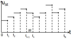
Figure 4: A sketch of $u_{\Delta t}$.

Our goal is to show that there exists a subsequence of the sequence of approximating solutions defined above, which converges to a weak solution of problem (9)-(14).

6 Convergence of approximate solutions

6.1 Weak and weak* convergence

We now focus on the sequences of approximate solutions $(\boldsymbol{\eta}_{\Delta t})_{\Delta t}$, $({\bf u}_{\Delta t})_{\Delta t}$, and $({\bf v}_{\Delta t})_{\Delta t}$, as $\Delta t\to 0$ (or, equivalently, as $N\to\infty$). We first show that these sequences are uniformly bounded, independently of $\Delta t$, in the appropriate function norms. The main ingredient in showing the uniform estimates will be the results of Proposition 4.

Proposition 5.

The sequence $(\boldsymbol{\eta}_{\Delta t})_{\Delta t}$ is uniformly bounded in $L^{\infty}(0,T;H_{0}^{2}(\Gamma))^{2}$. Moreover, there exists a $T$ small enough such that ${\bf A}_{\Delta t}^{n}$ is an injection, and

$$J^{n}_{\Delta t}=\det\nabla{\bf A}_{\Delta t}^{n}>0,\quad\Delta t>0,n=1,\dots N.$$

Proof.

From Proposition 4 we have that $E_{\Delta t}^{n}\leq C$, where $C$ is independent of $\Delta t$. This implies

$$\|\boldsymbol{\eta}_{\Delta t}\|_{L^{\infty}(0,T;H_{0}^{2}(\Gamma))}\leq C.$$

To show that ${\bf A}_{\Delta t}^{n}$ is injective we again use Theorem 5.5.-1 from [12], stated as Theorem 1 in this manuscript, in the analogous way as in Proposition 1. First, we fix $\Delta t$ and consider the $H^{2}_{0}$-norm of the difference between the initial data and the approximate solution at time $n\Delta t$, to notice that

$$\|\boldsymbol{\eta}^{n}_{\Delta t}-\boldsymbol{\eta}_{0}\|_{H_{0}^{2}(\Gamma)}\leq\|\boldsymbol{\eta}^{n}_{\Delta t}\|_{H_{0}^{2}(\Gamma)}+\|\boldsymbol{\eta}_{0}\|_{H_{0}^{2}(\Gamma)}\leq 2C,\;n=1,\dots,N.$$

Furthermore, we calculate

$$\|\boldsymbol{\eta}^{n}_{\Delta t}-\boldsymbol{\eta}_{0}\|_{L^{2}(\Gamma)}\leq\sum_{i=0}^{n-1}\|\boldsymbol{\eta}^{i+1}_{\Delta t}-\boldsymbol{\eta}^{i}_{\Delta t}\|_{L^{2}(\Gamma)}=\Delta t\sum_{i=0}^{n-1}\|{\bf v}^{i+\frac{1}{2}}_{\Delta t}\|_{L^{2}(\Gamma)}\leq CT,$$

where we used that $\boldsymbol{\eta}^{0}_{\Delta t}=\boldsymbol{\eta}_{0}$, and Proposition 4, estimate $E_{\Delta t}^{n+\frac{1}{2}}\leq C$, where $C$ is independent of $\Delta t$, to bound

$$\|\boldsymbol{\eta}^{n}_{\Delta t}-\boldsymbol{\eta}_{0}\|_{L^{2}(\Gamma)}\leq Cn\Delta t\leq CT,\;n=1,\dots,N.$$

Now, we have uniform bounds for $\|\boldsymbol{\eta}^{n}_{\Delta t}-\boldsymbol{\eta}_{0}\|_{L^{2}(\Gamma)}$ and $\|\boldsymbol{\eta}^{n}_{\Delta t}-\boldsymbol{\eta}_{0}\|_{H_{0}^{2}(\Gamma)}$. Therefore, we can use the interpolation inequality for Sobolev spaces (see for example [1], Thm. 4.17, p. 79) to get

$$\|\boldsymbol{\eta}^{n}_{\Delta t}-\boldsymbol{\eta}_{0}\|_{H^{11/6}(\Gamma)}\leq 2CT^{1/12},\;n=1,\dots,N.$$

Now from (23) and the construction of the ALE mapping we have

$$\|\nabla{\bf A}_{\Delta t}^{n}-{\bf I}\|_{C^{0,1/3}(\Omega)}\leq\tilde{C}\|\boldsymbol{\eta}^{n}_{\Delta t}\|_{H^{11/6}(\Gamma)}\leq\|\boldsymbol{\eta}_{0}\|_{H^{11/6}(\Gamma)}+2CT^{1/12},$$

where ${\bf I}$ is the identity matrix.

We want to show that the right hand-side is bounded by a constant which is smaller than or equal to the constant $c(\Omega)$ given by (31) in Theorem 1 (B), which guarantees injectivity of the ALE mapping. Indeed, from Proposition 4 we see that $C$ above depends on $T$ through the norms of the inlet and outlet data in such a way that $C$ is an increasing function of $T$. Therefore by choosing $T$ small, we can make $\|\boldsymbol{\eta}^{n}_{\Delta t}-\boldsymbol{\eta}_{0}\|_{H^{11/6}(\Gamma)}$ arbitrarily small for $n=1,.\dots,N$. Furthermore, by using the assumption (17) on the smallness of the initial domain displacement, we see that we can choose a $T^{\prime\prime}>0$ small enough, independent of $\Delta t$, such that there exists a constant $\tilde{c}>0$ giving

$$\|\nabla{\bf A}_{\Delta t}^{n}-{\bf I}\|_{C^{0,1/3}(\Omega)}\leq\tilde{c},$$

where $\tilde{c}$ is smaller than or equal to the constant $c(\Omega)$ from Theorem 1 (B), which implies injectivity of the ALE mapping $\nabla{\bf A}_{\Delta t}^{n}$.

Finally, from condition (16) requiring that the “initial” Jacobian of $\boldsymbol{\varphi}^{0}$ is strictly positive, we see that there exists a $T^{\prime}>0$ small, independent of $\Delta t$, such that the Jacobian $J_{\Delta t}^{n}$ is strictly positive. By taking

$$T={\rm min}\{T^{\prime},T^{\prime\prime}\},$$ (61)

we obtain the proof of the proposition. ∎

We note that it is this $T$, given by Proposition 5, that determines the time interval of existence of a weak solution to problem (9)-(14), since $T$ given in (61) is independent of $\Delta t$. The time given in (32) is a continuous version of the time given by (61).

Next, we show uniform boundedness of the approximating sequences for the fluid and structure velocities.

Proposition 6.

The following statements hold:

1. $({\bf v}_{\Delta t})_{\Delta t}$, $({\bf v}_{\Delta t}^{*})_{\Delta t}$ are uniformly bounded in $L^{\infty}(0,T;L^{2}(\Gamma))$,

2. $({\bf u}_{\Delta t})_{\Delta t}$ is uniformly bounded in $L^{\infty}(0,T;L^{2}(\Omega))\cap L^{2}(0,T;H^{1}(\Omega))$.

Proof.

The proof follows from Propositions 4 and 5 and from the uniform Korn’s inequality stated in Lemma 1. Namely, statement 2 of Proposition 4 implies that ${\bf D}^{\eta_{\Delta t}}({\bf u}_{\Delta t})$ is bounded in $L^{2}(0,T;L^{2}(\Omega))$. Now, we can use the uniform bound for $\boldsymbol{\eta}_{\Delta t}$ and the uniform Korn’s inequality from Lemma 1 to finish the proof. ∎

Lemma 2.

(Weak and weak* convergence results) There exist subsequences $(\boldsymbol{\eta}_{\Delta t})_{\Delta t},({\bf v}_{\Delta t})_{\Delta t},({\bf v}^{*}_{\Delta t})_{\Delta t},$ and $({\bf u}_{\Delta t})_{\Delta t}$, and the functions $\eta\in L^{\infty}(0,T;H^{2}_{0}(\Gamma))$, ${\bf v}\in L^{\infty}(0,T;L^{2}(\Gamma))$, ${\bf v}^{*}\in L^{\infty}(0,T;L^{2}(\Gamma))$, and ${\bf u}\in L^{\infty}(0,T;L^{2}(\Omega))\cap L^{2}(0,T;H^{1}(\Omega))$, such that

$$\begin{array}[]{rcl}\boldsymbol{\eta}_{\Delta t}&\rightharpoonup&\boldsymbol{\eta}\;{\rm weakly*}\;{\rm in}\;L^{\infty}(0,T;H^{2}_{0}(\Gamma)),\\ {\bf v}_{\Delta t}&\rightharpoonup&{\bf v}\;{\rm weakly*}\;{\rm in}\;L^{\infty}(0,T;L^{2}(\Gamma)),\\ {\bf v}^{*}_{\Delta t}&\rightharpoonup&{\bf v}^{*}\;{\rm weakly*}\;{\rm in}\;L^{\infty}(0,T;L^{2}(\Gamma)),\\ {\bf u}_{\Delta t}&\rightharpoonup&{\bf u}\;{\rm weakly*}\;{\rm in}\;L^{\infty}(0,T;L^{2}(\Omega)),\\ {\bf u}_{\Delta t}&\rightharpoonup&{\bf u}\;{\rm weakly}\;{\rm in}\;L^{2}(0,T;H^{1}(\Omega)).\end{array}$$ (62)

Furthermore,

$${\bf v}={\bf v}^{*}.$$ (63)

Since our problem is nonlinear, we need strong convergence of approximating sub-sequences to be able to pass to the limit, and show that the limiting functions satisfy the weak formulation of the problem. For this purpose we need a compactness result, which we present next.

6.2 Compactness

Compactness arguments in the case when the boundary condition on $\Gamma(t)$ is the slip condition is different from the compactness argument for the problem in which the boundary condition on $\Gamma(t)$ is no-slip. In the no-slip case the viscous dissipation of the fluid smooths out the interface providing spatial regularity of the interface velocity ${\bf v}_{\Delta t}$, which is no longer available in the slip condition case, since the fluid and structure velocities are no longer equal at the fluid-structure interface. We will have some help from the viscous fluid dissipation in the estimates for the normal component of structure velocity, but the tangential component no longer “feels” fluid dissipation as before. It is because of this that we need to construct a different compactness argument, which we present next.

To investigate compactness (regularization) in time we introduce the translation in time by $h$ of a function $f$, denoted by $T_{h}$, as:

$$T_{h}f(t,.)=f(t-h,.),\ h\in{\mathbb{R}}.$$ (64)

The following estimates hold for our approximate solutions as they are shifted in time by $h$:

Lemma 3.

There exists a constant $C>0$, independent of $\Delta t$, such that for every $h>0$ we have:

$$\|T_{h}{\bf u}_{\Delta t}-{\bf u}_{\Delta t}\|_{L^{2}(h,T;L^{2}(\Omega))}\leq C\sqrt{h},$$

$$\|T_{h}{\bf v}_{\Delta t}-{\bf v}_{\Delta t}\|_{L^{2}(h,T;L^{2}(\Gamma))}\leq C\sqrt{h},$$

$$\|T_{h}{\bf v}^{*}_{\Delta t}-{\bf v}^{*}_{\Delta t}\|_{L^{2}(h,T;L^{2}(\Gamma))}\leq C\sqrt{h},$$

$$\|T_{h}\boldsymbol{\eta}_{\Delta t}-\boldsymbol{\eta}_{\Delta t}\|_{L^{2}(h,T;H^{2}(\Gamma))}\leq C\sqrt{h},\;\Delta t>0.$$

Proof.

The proof is analogous to the proof of Theorem 2 in [42]. A summary of the main steps is the following. We focus on the first statement given in terms of ${\bf u}_{\Delta t}$, while the proofs for the other two are analoguous. First, from Proposition 4 we immediately have:

$$\|T_{\Delta t}{\bf u}_{\Delta t}-{\bf u}_{\Delta t}\|_{L^{2}(\Delta t,T;L^{2}(\Omega))}^{2}=\sum_{n}\|{\bf u}_{\Delta t}^{n+1}-{\bf u}_{\Delta t}^{n}\|^{2}_{L^{2}(\Omega)}\Delta t\leq C\Delta t.$$

This implies that the first estimate in the above Lemma holds for “the diagonal” terms for which the translation is performed by $h$ that is exactly equal to $\Delta t$. However, we would like to prove the statement for an arbitrary translation by $h>0$. Let us fix $\Delta t>0$ and consider the following two cases: $0<h<\Delta t$ and $0<\Delta t<h$. We obtain the desired estimates by calculating the following.

1. For $0<h<\Delta t$ we have

   $$\|T_{h}{\bf u}_{\Delta t}-{\bf u}_{\Delta t}\|_{L^{2}(h,T;L^{2}(\Omega))}^{2}=\sum_{n}\int_{n\Delta t-h}^{n\Delta t}\|{\bf u}_{\Delta t}^{n+1}-{\bf u}_{\Delta t}^{n}\|^{2}_{L^{2}(\Omega)}$$

   $$=h\sum_{n}\|{\bf u}_{\Delta t}^{n+1}-{\bf u}_{\Delta t}^{n}\|^{2}_{L^{2}(\Omega)}\leq Ch.$$

2. For $0<\Delta t<h$ we write $h=l\Delta t+s$ for some $l\in{\mathbb{N}}$ and $0\leq s<\Delta t$, and use the triangle inequality to get

   $$\|T_{h}{\bf u}_{\Delta t}-{\bf u}_{\Delta t}\|_{L^{2}(h,T;L^{2}(\Omega))}^{2}\leq\Delta t\sum_{n}\sum_{i=1}^{l+1}\|{\bf u}_{\Delta t}^{j+i-1}-{\bf u}_{\Delta t}^{j+i}\|^{2}_{L^{2}\Gamma}\leq C(l+1)\Delta t\leq Ch.$$

∎

In what follows, it will be useful to introduce a slightly different set of approximate functions for $\mathbf{u}$, $v$, and $\eta$ by extending the values of those functions at points $n\Delta t$ to the time sub-interval $[(n-1)\Delta t,n\Delta t]$ not in a piece-wise constant fashion as before, but linearly. Namely, for each fixed $\Delta t$, define $\tilde{\bf u}_{N}$, $\tilde{\boldsymbol{\eta}}_{\Delta t}$ and $\tilde{{\bf v}}_{\Delta t}$ to be continuous, linear on each sub-interval $[(n-1)\Delta t,n\Delta t]$, and such that

$$\tilde{\bf u}_{\Delta t}(n\Delta t,.)={\bf u}_{\Delta t}(n\Delta t,.),\ \tilde{{\bf v}}_{\Delta t}(n\Delta t,.)={{\bf v}}_{\Delta t}(n\Delta t,.),\ \tilde{\boldsymbol{\eta}}_{\Delta t}(n\Delta t,.)={\boldsymbol{\eta}}_{\Delta t}(n\Delta t,.),$$ (65)

where $n=0,\dots N$. We now observe that

$${\tilde{\boldsymbol{\eta}}_{\Delta t}(t)=\frac{\boldsymbol{\eta}^{n+1}-\boldsymbol{\eta}^{n}}{\Delta t}(t-n\Delta t)+\boldsymbol{\eta}^{n},\quad t\in[n\Delta t,(n+1)\Delta t),\;n=0,\dots,N-1,}$$ (66)

$${\partial_{t}\tilde{\boldsymbol{\eta}}_{\Delta t}(t)=\frac{\boldsymbol{\eta}^{n+1}-\boldsymbol{\eta}^{n}}{\Delta t}=\frac{\boldsymbol{\eta}^{n+1/2}-\boldsymbol{\eta}^{n}}{\Delta t}={\bf v}^{n+\frac{1}{2}}},\ t\in(n\Delta t,(n+1)\Delta t),$$

and so, since ${\bf v}^{*}_{\Delta t}$ was defined in (60) as a piece-wise constant function defined via $v^{*}_{\Delta t}(t,\cdot)=v^{n+\frac{1}{2}}$, for $t\in(n\Delta t,(n+1)\Delta t]$, we see that

$$\partial_{t}\tilde{\boldsymbol{\eta}}_{\Delta t}={\bf v}^{*}_{\Delta t}\ a.e.\ {\rm on}\ (0,T).$$ (67)

The following Lemma will be crucial for establishing compactness of the approximate sequence of solutions $\tilde{\boldsymbol{\eta}}_{\Delta t}$.

Lemma 4.

There exists a constant $C>0$, independent of $\Delta t$, such that for every $h>0$ we have:

$$\|T_{h}{\tilde{\boldsymbol{\eta}}}_{\Delta t}-{\tilde{\boldsymbol{\eta}}}_{\Delta t}\|_{L^{2}(h,T;H^{2}(\Gamma))}\leq C\sqrt{h}.$$

Proof.

In the same way as in Lemma 3 we consider two separate cases: $0<h\leq\Delta t$ and $\Delta t<h.$

Case 1: $0<h\leq\Delta t$. We use (66) and explicitly calculate the straight lines defining the function $\tilde{\boldsymbol{\eta}}_{\Delta t}$ and its translation in time by $h$ to the right, to obtain:

$$\int_{h}^{T}\|T_{h}{\tilde{\boldsymbol{\eta}}}_{\Delta t}-{\tilde{\boldsymbol{\eta}}}_{\Delta t}\|_{H^{2}(\Gamma)}^{2}=\int_{h}^{\Delta t}\|\frac{\boldsymbol{\eta}^{1}_{\Delta t}-\boldsymbol{\eta}_{0}}{\Delta t}(-h)\|_{H^{2}(\Gamma)}^{2}\ dt$$

$$+\sum_{n=1}^{N-1}\Big{\{}\int_{n\Delta t}^{n\Delta t+h}\Big{(}\frac{1}{\Delta t^{2}}\|h(\boldsymbol{\eta}_{\Delta t}^{n}-\boldsymbol{\eta}_{\Delta t}^{n+1})+(n\Delta t-t)(\boldsymbol{\eta}_{\Delta t}^{n+1}-2\boldsymbol{\eta}_{\Delta t}^{n}+\boldsymbol{\eta}_{\Delta t}^{n-1})\|_{H^{2}(\Gamma)}^{2}\Big{)}dt$$

$$+\int^{(n+1)\Delta t}_{n\Delta t+h}\|\frac{\boldsymbol{\eta}_{\Delta t}^{n+1}-\boldsymbol{\eta}_{\Delta t}^{n}}{\Delta t}(-h)\|_{H^{2}(\Gamma)}^{2}dt\Big{\}}\leq C(\frac{h^{3}}{\Delta t^{2}}+\frac{h^{2}}{\Delta t})\sum_{n=0}^{N-1}\|\boldsymbol{\eta}_{\Delta t}^{n+1}-\boldsymbol{\eta}_{\Delta t}^{n}\|^{2}_{H^{2}(\Gamma)}\leq Ch.$$

The last inequality follows from Proposition 4 and from the fact that $h\leq\Delta t$.

Case 2: $\Delta t<h$. We notice that $T_{h}\tilde{\boldsymbol{\eta}}_{\Delta t}=\widetilde{T_{h}\boldsymbol{\eta}_{\Delta t}}$ and use the following identity (see e.g. [55], p. 328)

$$\|\boldsymbol{\eta}_{\Delta t}-\tilde{\boldsymbol{\eta}}_{\Delta t}\|^{2}_{L^{2}(0,T;H^{2}(0,L))}\leq{\frac{\Delta t}{3}}\sum_{n=0}^{N-1}\|\boldsymbol{\eta}^{n+1}_{\Delta t}-\boldsymbol{\eta}^{n}_{\Delta t}\|^{2}_{H^{2}(0,L)}.$$

From Lemma 3 we have:

$$\|T_{h}{\tilde{\boldsymbol{\eta}}}_{\Delta t}-{\tilde{\boldsymbol{\eta}}}_{\Delta t}\|_{L^{2}(h,T;H^{2}(\Gamma))}\leq\|\widetilde{T_{h}\boldsymbol{\eta}_{\Delta t}}-T_{h}\boldsymbol{\eta}_{\Delta t}\|_{L^{2}(0,T;H^{2}(0,L))}$$

$$+\|T_{h}\boldsymbol{\eta}_{\Delta t}-\boldsymbol{\eta}_{\Delta t}\|_{L^{2}(0,T;H^{2}(0,L))}+\|\boldsymbol{\eta}_{\Delta t}-\tilde{\boldsymbol{\eta}}_{\Delta t}\|_{L^{2}(0,T;H^{2}(0,L))}\leq C(\Delta t+h+\Delta t)\leq Ch.$$

The statement of the Lemma immediately follows by taking the square root on both sides of the inequality. ∎

Proposition 7.

The following statements hold:

1. $({\bf u}_{\Delta t})_{\Delta t>0}$ is uniformly bounded in $H^{s}(0,T;L^{2}(\Omega))$, $0\leq s<1/2$.

2. $({\tilde{\boldsymbol{\eta}}}_{\Delta t})_{\Delta t>0}$ is uniformly bounded in $H^{s}(0,T;H^{2}(\Gamma))\cap H^{s+1}(0,T;L^{2}(\Gamma))$, $0\leq s<1/2$.

3. $({\bf v}^{*}_{\Delta t})_{\Delta t>0}$ is uniformly bounded in $H^{s}(0,T;L^{2}(\Gamma))\cap L^{2}(0,T;H^{2s}(\Gamma))$, $0\leq s<1/2$.

Proof.

Since we have already proved that ${\bf u}_{\Delta t}$ is uniformly bounded in $L^{2}(0,T;L^{2}(\Omega))$, it only remains to prove that the following semi-norm is finite:

$$\|{\bf u}_{\Delta t}\|_{H^{s}(0,T;L^{2}(\Omega))}^{2}=\int_{0}^{T}\int_{0}^{T}\frac{\|{\bf u}_{\Delta t}(t)-{\bf u}_{\Delta t}(\tau)\|_{L^{2}(\Omega)}^{2}}{|t-\tau|^{1+2s}}dtd\tau.$$

By a simple change of variables $h=t-\tau$ and Lemma 3 we get:

$$\|{\bf u}_{\Delta t}\|_{H^{s}(0,T;L^{2}(\Omega))}^{2}=\int_{-T}^{T}\frac{dh}{|h|^{1+2s}}\int_{0}^{T}\|{\bf u}_{\Delta t}(t-h)-{\bf u}_{\Delta t}(t)\|_{L^{2}({\Omega})}^{2}d\tau\leq\int_{-T}^{T}\frac{|h|dh}{|h|^{1+2s}}.$$

This integral is finite for $s<1/2$ and therefore we have proved the first statement.

The first part of the second statement and the first part of the third statement, i.e. $({\tilde{\boldsymbol{\eta}}}_{\Delta t})_{\Delta t>0}$ and $({\bf v}^{*}_{\Delta t})_{\Delta t>0}$ are uniformly bounded in $H^{s}(0,T;H^{2}(\Gamma))$ and $H^{s}(0,T;L^{2}(\Gamma))$, $0\leq s<1/2$, respectively, are proved analogously by using Lemma 3 again.

Let us now prove the boundedness of $({\bf v}^{*}_{\Delta t})_{\Delta t>0}$ in $L^{2}(0,T;H^{2s}(\Gamma))$. First notice that from (67) and the uniform boundedness of $({\bf v}^{*}_{\Delta t})_{\Delta t>0}$ in $H^{s}(0,T;L^{2}(\Gamma))$, $s<1/2$ that we just proved, we see that $(\partial_{t}{\tilde{\boldsymbol{\eta}}}_{\Delta t})$ is uniformly bounded in $H^{s}(0,T;L^{2}(\Gamma))$, $s<1/2$. Therefore,

$$({\tilde{\boldsymbol{\eta}}}_{\Delta t})\;{\rm is\;uniformly\;bounded\;in}\;H^{s+1}(0,T;L^{2}(\Gamma))\cap H^{s}(0,T;H^{2}(\Gamma)),\;s<1/2.$$

Now, by the interpolation property (see e.g. [39] Section 1.9.4 p.p. 47) we obtain that $({\tilde{\boldsymbol{\eta}}}_{\Delta t})$ is uniformly bounded in $H^{1}(0,T;H^{2s}(\Gamma))$. By using (67) again we conclude that $({\bf v}^{*}_{\Delta t})_{\Delta t>0}=(\partial_{t}\tilde{\boldsymbol{\eta}}_{\Delta t})$ is uniformly bounded in $L^{2}(0,T;H^{2s}(\Gamma))$, $s<1/2$. ∎

Notice that the proof of this Proposition heavily relies on the definition of the new approximate solution sequences (65) and their properties (66) and (67). In particular, (67) allowed us to obtain information about the regularity properties of $({\bf v}^{*}_{\Delta t})_{\Delta t>0}$ via the regularity of $(\partial_{t}{\tilde{\boldsymbol{\eta}}}_{\Delta t})$. It is because of this result that we introduced the new definition of approximate solutions given by (65). We shall see below that the limits of approximate sequences as $\Delta t\to 0$ do not depend on the type of extension of the approximate values of the solution at points $n\Delta t$ onto the time sub-interval $(n\Delta t,(n+1)\Delta t)$. Therefore, the introduction of the new approximate sequences in (65) to obtain additional information about the regularity of the limiting solution is justified.

We note here a side remark that we could have proved Proposition 7 by using a slightly different but equivalent approach, relying on Nikolskii spaces. More precisely, from Lemma 3 we can directly conclude that sequences $({\bf u})_{\Delta t}$, ${(\bf v})_{\Delta t}$, $({\bf v})^{*}_{\Delta t}$, $(\boldsymbol{\eta})_{\Delta t}$ are uniformly bounded in the following Nikolskii spaces $N^{1/2,2}((0,T);L^{2}(\Omega))$, $N^{1/2,2}((0,T);L^{2}(\Gamma))$ and $N^{1/2,2}((0,T);H^{2}(\Gamma))$, respectively (see e.g. [54] for the definition of the Nikolskii spaces). Similarly, Lemma 4 gives uniform boundedness of $(\tilde{\boldsymbol{\eta}})_{\Delta t}$ in $N^{1/2,2}((0,T);H^{2}(\Gamma))$. Proposition 7 then follows directly from the embeddings of Nikolskii spaces into $H^{s}$ spaces [54].

We are now ready to state our main compactness result. It relies on the following compactness theorem by Simon, stated in [53] as Corollary 5.

Theorem 3.

(Corollary 5 [53]) Assume that $X$, $B$, and $Y$ are Banach spaces, and $X\subset B\subset Y$ with compact embedding $X\subset\subset B$. Let $1\leq p\leq\infty$ and $1\leq r\leq\infty$. Let $F$ be bounded in $L^{p}(0,T;X)\cap W^{s,r}(0,T;Y)$, where $s>0$ if $r\geq p$, and where $s>1/r-1/p$ if $r<p$. Then $F$ is relatively compact in $L^{p}(0,T;B)$ (and in $C(0,T;B)$ if $p=\infty$).

Theorem 4.

(Compactness) Sets $\{{\bf u}_{\Delta t}:\Delta t>0\}$ and $\{{\bf v^{*}}_{\Delta t}:\Delta t>0\}$ are relatively compact in $L^{2}(0,T;H^{2s}(\Omega))$, $s<1/2$, and $L^{2}(0,T;H^{2s}(\Gamma))$, respectively.

Proof.

The proof of this theorem follows from the estimates obtained in Propositions 6 and 7, and by applying Theorem 3 with $p=r=2$ and $s>0$. ∎

We remark that in contrast with the no-slip condition case studied in [42], where we obtained partial regularity of $\partial_{t}\eta$ from the trace of the fluid velocity on the interface and the estimates related to the fluid viscous dissipation, here we had to calculate directly all the time-shifts for $\boldsymbol{\eta}_{\Delta t},{\bf u}_{\Delta t}$, and ${\bf v}_{\Delta t}$, and ${\bf v}^{*}_{\Delta t}$ to obtain uniform boundedness in the $H^{s}$ spaces which, combined with the Simon’s Corollary 5 and interpolation of classical Sobolev spaces $H^{s}$ with real exponents $s$, provide compactness.

The compactness result stated in Theorem 4 implies the following strong convergence results.

Corollary 1.

We have the following strong convergence results as $\Delta t\to 0$:

1. ${\bf u}_{\Delta t}\to{\bf u}\quad{\rm in}\ L^{2}(0,T;H^{2s}(\Omega)),\ s<1/2,$

2. ${\bf v}^{*}_{\Delta t}\to{\bf v}\quad{\rm in}\ L^{2}(0,T;H^{2s}(\Gamma)),\ s<1/2,$

3. ${\bf v}_{\Delta t}\to{\bf v}\quad{\rm in}\ L^{2}(0,T;H^{2s}(\Gamma)),\ s<1/2.$

To get strong convergence results for the structure displacements $\boldsymbol{\eta}_{\Delta t}$ we proceed in the same way as in [42]. Namely, from Propositions 5 and 6, and from $\partial\tilde{\boldsymbol{\eta}}_{\Delta t}={\bf v}^{*}_{\Delta t}$, we obtain that $\tilde{\boldsymbol{\eta}}_{\Delta t}$ is uniformly bounded in $L^{\infty}(0,T;H_{0}^{2}(\Gamma))^{2}\cap W^{1,\infty}(0,T;L^{2}(\Gamma))^{2}$. From the continuous embedding

$$L^{\infty}(0,T;H_{0}^{2}(\Gamma))^{2}\cap W^{1,\infty}(0,T;L^{2}(\Gamma))^{2}\hookrightarrow C^{0,1-\alpha}([0,T],H^{2\alpha}(\Gamma)),\ 0<\alpha<1,$$

we obtain uniform boundedness of $\tilde{\boldsymbol{\eta}}_{\Delta t}$ in $C^{0,1-\alpha}([0,T],H^{2\alpha}(\Gamma))$. Now, to get compactness in space we recall that $H^{2\alpha}$ is continuously embedded into $H^{2\alpha-\epsilon}$. By the Arzelà-Ascoli theorem this embedding is compact. In fact, by the application of the Arzelà-Ascoli theorem to the functions in $C^{0,1-\alpha}([0,T],H^{2\alpha}(\Gamma))$ we get the compactness is time as well. More precisely, we obtain the existence of a subsequence, which we denote by $\tilde{\boldsymbol{\eta}}_{\Delta t}$ again, such that

$$\tilde{\boldsymbol{\eta}}_{\Delta t}\to\tilde{\boldsymbol{\eta}}\quad{\rm in}\quad C([0,T];H^{2s}(\Gamma)),\ 0<s<1.$$

Since sequences $\tilde{\boldsymbol{\eta}}_{\Delta t}$ and $\boldsymbol{\eta}_{\Delta t}$ have the same limit $\tilde{\boldsymbol{\eta}}=\boldsymbol{\eta}\in C([0,T];H^{2s}(\Gamma))$, where $\boldsymbol{\eta}$ is the weak* limit discussed in Lemma 2, we obtain

$$\tilde{\boldsymbol{\eta}}_{\Delta t}\to\boldsymbol{\eta}\quad{\rm in}\quad C([0,T];H^{2s}(\Gamma)),\ 0<s<1.$$

By combining this statement with the continuity in time of $\boldsymbol{\eta}$, as was done in Lemma 3 of [42], we obtain the following strong convergence results for the structure:

Theorem 5.

The following strong convergence results hold as $\Delta t\to 0$:

1. $\displaystyle{\boldsymbol{\eta}_{\Delta t}\to\boldsymbol{\eta}\;{\rm in}\;L^{\infty}(0,T;H^{2s}(\Gamma))}$, $s<1$,

2. $\displaystyle{T_{\Delta t}\boldsymbol{\eta}_{\Delta t}\to\boldsymbol{\eta}\;{\rm in}\;L^{\infty}(0,T;H^{2s}(\Gamma))}$, $s<1$.

To pass to the limit in the weak formulation, we need uniform convergence of $\boldsymbol{\eta}_{\Delta t}$. This is where the fact that we work in 2D rather than in 3D comes into play. Namely, since in our 2D problem $\Gamma$ is a 1D domain, we have that $H^{\alpha}(\Gamma)$ is embedded into $C^{1}(\overline{\Gamma})$ for $s>3/2$, and so the first statement of Theorem 5 implies $\displaystyle{\boldsymbol{\eta}_{\Delta t}\to\boldsymbol{\eta}\;{\rm in}\;L^{\infty}(0,T;C^{1}(\overline{\Gamma}))}$. Moreover, we have the following Corollary.

Corollary 2.

The following uniform convergence results hold as $\Delta t\to 0$:

1. $\displaystyle{\boldsymbol{\eta}_{\Delta t}\to\boldsymbol{\eta}\;{\rm in}\;L^{\infty}(0,T;C^{1}(\overline{\Gamma}))}$,

2. $\displaystyle{T_{\Delta t}\boldsymbol{\eta}_{\Delta t}\to\boldsymbol{\eta}\;{\rm in}\;L^{\infty}(0,T;C^{1}(\overline{\Gamma}))}$.

The second statement in this corollary can be proved using the same arguments as those following statement (76) in [42].

By using this corollary, and the explicit formulas for the normals $\boldsymbol{\nu}_{\Delta t}$, the tangents $\boldsymbol{\tau}_{\Delta t}$, and the quantities associated with the ALE mappings ${\bf A}_{\Delta t}$, one can see that the following strong convergence results hold:

Corollary 3.

The following strong convergence results hold for the geometric quantities associated with the change of the fluid domain $\Omega(t)$:

1. $\boldsymbol{\nu}_{\Delta t}\to\boldsymbol{\nu}^{\eta}\;{\rm in}\;L^{\infty}(0,T;C(\overline{\Gamma}))$,

2. $\boldsymbol{\tau}_{\Delta t}\to\boldsymbol{\tau}^{\eta}\;{\rm in}\;L^{\infty}(0,T;C(\overline{\Gamma}))$,

3. ${\bf w}_{\Delta t}\to{\bf w}^{\eta}\;{\rm in}\;L^{2}(0,T;H^{1}(\Omega))$,

4. $S_{\Delta t}\to S^{\eta}\;{\rm in}\;L^{\infty}(0,T;C(\overline{\Gamma}))$,

5. $J_{\Delta t}\to J^{\eta}\;{\rm in}\;L^{\infty}(0,T;C(\overline{\Omega}))$,

6. $(\nabla{\bf A}_{\Delta t})^{-1}\to(\nabla{\bf A}_{\eta})^{-1}\;{\rm in}\;L^{\infty}(0,T;C(\overline{\Omega}))$.

We remark that the results of Corollary 3 were not necessary in our previous work [42] because only the normal component of structure displacement was assumed to be non-zero. In the current manuscript both the normal and tangential structure displacements are considered to be non-zero, which introduces additional complications in tracking the change in the measure of the interface “surface” deformation that we did not have to deal with before.

7 The limiting problem

7.1 Construction of suitable test functions

Now that we have the strong convergence results above, we are ready to show that the limits, as $\Delta t\to 0$, of approximate solutions satisfy the weak form (43) of problem (9)-(14). Unfortunately, due to the fact that we mapped our problem defined on the moving domain $\Omega(t)$ onto a fixed, reference domain $\Omega$, introduces additional difficulties. More precisely, the velocity test functions in the weak formulation of the fluid sub-problem (57) now depend of $\Delta t$ via their dependence on $\eta^{n}_{\Delta t}$. This is because of the requirement that the transformed divergence-free condition $\nabla^{\eta^{n}_{\Delta t}}\cdot{\bf q}=0$ must be satisfied. Passing to the limit in the weak formulation of the fluid sub-problem (57) when both the test functions and the unknown functions depend on $\Delta t$ is tricky, and special care needs to be taken to deal with this issue.

Our strategy is to restrict ourselves to a dense subset, call it ${\mathcal{X}}^{\eta}(0,T)$, of the space of all test functions ${\mathcal{Q}}^{\eta}(0,T)$, and for every ${\bf q}\in{\mathcal{X}}^{\eta}(0,T)$ construct a sequence of test functions for the approximate problems, call them ${\bf q}_{\Delta t}$, such that ${\bf q}_{\Delta t}\to{\bf q}$ in suitable norms. This approach was used in [42] for the FSI problem with the no-slip condition and only radial structural displacements, see also [10, 43, 44]. Since, here the test space is different because of the slip boundary condition, the construction of such test functions is somewhat different.

First let us define the domain which contains all the approximate domains

$${\Omega_{\rm max}=\bigcup_{\Delta t>0,n\in{\mathbb{N}}}\Omega^{\eta^{n}_{\Delta t}}}.$$ (68)

Notice that Corollary 2 implies $\Omega^{\eta}(t)\subset\Omega_{\rm max}$, $t\in[0,T]$, and $\Sigma\subset\partial\Omega_{\rm max}$. We define

$${\mathcal{X}}_{\rm max}= \{{\bf r}\in C^{1}_{c}([0,T);C^{2}(\overline{\Omega}_{\rm max}))^{2}:\nabla\cdot{\bf r}=0,{\bf r}\cdot\boldsymbol{\tau}=0,\;{\rm on}\ \Gamma_{i},\;i\in I,\;{\bf r}=0\ {\rm on}\ \Gamma_{i},\;i\in II,\;$$

$$\ \ {\bf r}\cdot\boldsymbol{\nu}=0,\;{\rm on}\ \Gamma_{i},\;i\in III\cup IV\}.$$

$${\mathcal{X}}^{\eta}(0,T)= \{({\bf q},\boldsymbol{\psi}):{\bf q}(t,.)={\bf r}(t,.)_{|\Omega^{\eta}(t)}\circ{\bf A}_{\eta}(t),{\bf r}\in{\mathcal{X}}_{\rm max},\;({\bf r}_{|\Gamma^{\eta}}-\boldsymbol{\psi})\cdot\boldsymbol{\nu}^{\eta}=0,\;\boldsymbol{\psi}\in H^{2}_{0}(\Gamma)\}.$$

From the construction it is immediate that ${\mathcal{X}}^{\eta}(0,T)$ is dense in ${\mathcal{Q}}^{\eta}(0,T)$.

We now want to construct the test functions ${\bf q}_{\Delta t}$ and ${\boldsymbol{\psi}}_{\Delta t}$ for the approximate problems, such that ${\bf q}_{\Delta t}\to{\bf q}$ and ${\boldsymbol{\psi}}_{\Delta t}\to\boldsymbol{\psi}$ in a suitable space. For this purpose let us fix $({\bf q},\boldsymbol{\psi})\in{\mathcal{X}}^{\eta}(0,T)$, ${\bf q}(t,.)={\bf r}(t,.)_{|\Omega^{\eta}(t)}\circ{\bf A}_{\eta}(t),\;{\bf r}\in{\mathcal{X}}_{\rm max}$, and define $({\bf q}_{\Delta t},{\boldsymbol{\psi}}_{\Delta t})$ to be piece-wise constant in time so that:

$$\left.\begin{array}[]{c}{\bf q}_{\Delta t}(t,.)={\bf q}^{n}_{\Delta t}:={\bf r}(n\Delta t,.)_{|\Omega^{\eta_{\Delta t}}(t)}\circ{\bf A}^{n}_{\Delta t}(t),\\ \\ \boldsymbol{\psi}_{\Delta t}(t)=\boldsymbol{\psi}^{n}_{\Delta t}:=\boldsymbol{\psi}(n\Delta t),\end{array}\right\},\;t\in((n-1)\Delta t,n\Delta t].$$ (69)

Note that $({\bf q}_{\Delta t}(t,.),\boldsymbol{\psi}_{\Delta t}(t,.))\in{\mathcal{V}}^{n}_{\Delta t}$, $t\in((n-1)\Delta t,n\Delta t]$. Now, using ideas from [42] we can prove the following lemma.

Lemma 5.

For every $({\bf q},\boldsymbol{\psi})\in{\mathcal{X}}^{\eta}(0,T)$ we have

$$({\bf q}_{\Delta t},\boldsymbol{\psi}_{\Delta t})\to({\bf q},\boldsymbol{\psi})\;{\rm in}\;L^{\infty}(0,T;C^{1}(\overline{\Omega}))^{2}\times L^{\infty}(0,T;C^{1}(\overline{\Gamma}))^{2}.$$

We will also need information about the convergence of approximations of $\partial_{t}{\bf q}$, which we define by:

$$d{\bf q}_{\Delta t}(t,.):=\frac{{\bf q}^{n+2}_{\Delta t}-{\bf q}^{n+1}_{\Delta t}}{\Delta t},\quad t\in((n-1)\Delta t,n\Delta t].$$ (70)

Lemma 6.

Let $({\bf q},\boldsymbol{\psi})\in{\mathcal{X}}^{\eta}(0,T)$, and let $d{\bf q}_{\Delta t}$ be defined by (70). Then $d{\bf q}_{\Delta t}\to\partial_{t}{\bf q}$ in $L^{2}(0,T;L^{2}(\Omega))$.

Proof.

By the Mean-Value Theorem we have

$$\frac{{\bf q}^{n+2}_{\Delta t}-{\bf q}^{n+1}_{\Delta t}}{\Delta t} =\frac{1}{\Delta t}\Big{(}{\bf r}\big{(}(n+2)\Delta t,{\bf A}^{n+2}_{\Delta t}(r,z)\big{)}-\big{(}(n+1)\Delta t,{\bf A}^{n+1}_{\Delta t}(r,z)\big{)}\Big{)}$$

$$=\frac{1}{\Delta t}\Big{(}{\bf r}\big{(}(n+2)\Delta t,{\bf A}^{n+2}_{\Delta t}(r,z)\big{)}-{\bf r}\big{(}(n+1)\Delta t,{\bf A}^{n+2}_{\Delta t}(r,z)\big{)}+$$

$$\qquad\quad\ {\bf r}\big{(}(n+1)\Delta t,{\bf A}^{n+2}_{\Delta t}(r,z)\big{)}-\big{(}(n+1)\Delta t,{\bf A}^{n+1}_{\Delta t}(r,z)\big{)}\Big{)}$$

$$=\partial_{t}{\bf r}\big{(}(n+1+\beta)\Delta t,{\bf A}^{n+2}_{\Delta t}(r,z)\big{)})+\nabla{\bf r}\big{(}(n+1)\Delta t,\boldsymbol{\zeta}\big{)}\frac{{\bf A}^{n+2}_{\Delta t}(r,z)-{\bf A}^{n+1}_{\Delta t}(r,z)}{\Delta t},$$

where $\boldsymbol{\zeta}={\bf A}^{n+1}_{\Delta t}(r,z)+\gamma({\bf A}^{n+2}_{\Delta t}(r,z)-{\bf A}^{n+1}_{\Delta t}(r,z))$, $\beta,\gamma\in[0,1]$. Notice that $\displaystyle{\frac{{\bf A}^{n+2}_{\Delta t}-{\bf A}^{n+1}_{\Delta t}}{\Delta t}={\bf w}^{n+2}_{\Delta t}}$, and this term is associated with $T_{-\Delta t}{\bf w}_{\Delta t}$, which converges strongly to ${\bf w}^{\eta}$ in $L^{2}(0,T;L^{2}(\Omega))$. Therefore we have

$$d{\bf q}_{\Delta t}\to\partial_{t}{\bf r}+\nabla{\bf r}\cdot{\bf w}^{\eta}=\partial_{t}{\bf q}\;{\rm in}\;L^{2}(0,T;L^{2}(\Omega)).$$

∎

7.2 Approximate equations

We have so far introduced the weak formulation of the coupled problem at the continuous level, and have split the coupled problem into the fluid and structure sub-problems. We then semi-discretized the two sub-problems, and introduced the semi-discrete weak formulations of those approximate fluid and structure sub-problems. What needs to be done next is to define the semi-discrete weak formulation of the coupled problem which approximates the weak formulation of the coupled continuous problem. To do that we take the constructed approximate test functions $({\bf q}_{\Delta t},\boldsymbol{\psi}_{\Delta t})$, multiply them by $\Delta t$, and replace the test functions ${\bf q}$ and $\boldsymbol{\psi}$ in the weak formulations for the approximate structure and fluid sub-problems  (50) and (57) with the test functions $\Delta t({\bf q}_{\Delta t},\boldsymbol{\psi}_{\Delta t})$. We add the two weak formulations together, and sum w.r.t. $n=0,\dots,N-1$. The approximating solutions $({\bf u}_{\Delta t},\boldsymbol{\eta}_{\Delta t})$ satisfy the following variational form of the semi-discretized (approximate) coupled problem:

$$\begin{array}[]{c}\displaystyle{\rho_{F}\int_{0}^{T}\int_{\Omega}T_{\Delta t}J_{\Delta t}\partial_{t}\tilde{\bf u}_{\Delta t}\cdot{\bf q}_{\Delta t}+\frac{\rho_{F}}{2}\int_{0}^{T}\int_{\Omega}\frac{J_{\Delta t}-T_{\Delta t}J_{\Delta t}}{\Delta t}{\bf u}_{\Delta t}\cdot{\bf q}_{\Delta t}}\\ \\ +\displaystyle{\frac{\rho_{F}}{2}\int_{0}^{T}\int_{\Omega}J_{\Delta t}\Big{(}((T_{\Delta t}{\bf u}_{\Delta t}-{\bf w}_{\Delta t})\cdot\nabla^{\eta_{\Delta t}}){\bf u}_{\Delta t}\cdot{\bf q}_{\Delta t}}\displaystyle{-((T_{\Delta t}{\bf u}_{\Delta t}-{\bf w}_{\Delta t})\cdot\nabla^{\eta_{\Delta t}}){\bf q}_{\Delta t}\cdot{\bf u}_{\Delta t}\Big{)}}\\ \\ \displaystyle{+2\mu\int_{0}^{T}\int_{\Omega}J_{\Delta t}{\bf D}^{\eta_{\Delta t}}({\bf u}_{\Delta t}):{\bf D}^{\eta_{\Delta t}}({\bf q}_{\Delta t})+\frac{1}{\alpha}\int_{0}^{T}\int_{\Gamma}(({\bf u}_{\Delta t}-{\bf v}_{\Delta t})\cdot\boldsymbol{\tau}_{\Delta t})({\bf q}_{\Delta t}\cdot\boldsymbol{\tau}_{\Delta t})S_{\Delta t}dz}\\ \\ \displaystyle{+\frac{1}{\alpha}\int_{0}^{T}\int_{\Gamma}(({\bf v}_{\Delta t}-{\bf u}_{\Delta t})\cdot\boldsymbol{\tau}_{\Delta t})({\boldsymbol{\psi}}_{\Delta t}\cdot\boldsymbol{\tau}_{\Delta t})S_{\Delta t}dz}\displaystyle{+\sum_{i\in III}\int_{\Gamma_{i}}\frac{1}{\alpha_{i}}({\bf u}_{\Delta t}\cdot\boldsymbol{\tau})({\bf q}_{\Delta t}\cdot\boldsymbol{\tau})}\\ \\ +\displaystyle{\rho_{S}h\int_{0}^{T}\int_{\Gamma}\partial_{t}\tilde{\bf v}_{\Delta t}\boldsymbol{\psi}_{\Delta t}}+\langle{\cal L}_{e}\boldsymbol{\eta}_{\Delta t},\boldsymbol{\psi}_{\Delta t}\rangle=\langle{\bf R}_{\Delta t},{\bf q}_{\Delta t}\rangle,\quad({\bf q},\boldsymbol{\psi})\in{\mathcal{X}}^{\eta}(0,T).\end{array}$$ (71)

We want to pass to the limit as $\Delta t\to 0$ and show that the limiting functions satisfy the weak formulation of problem (9)-(14), given in (43). Indeed, by using the convergence results for the approximate solutions given by Theorem 4, and Corollaries 2 and 3, and by using the convergence results for the corresponding test functions, given by Lemma 5, we can pass to the limit directly in all the terms, expect the ones associated with the geometric conservation law of the ALE mapping, i.e. the first two terms in the first line in (71).

7.3 Discrete v.s. continuous geometric conservation law

We show that the terms associated with the semi-discrete approximation of the geometric conservation law associated with our family of ALE mappings $A_{\Delta t}^{n}$, converge, as $\Delta t\to 0$, to the corresponding terms associates with the geometric conservation law satisfied by the ALE mapping $A^{\eta}$ appearing in the continuous weak formulation (43). More precisely, we have the following result.

Proposition 8.

For every $({\bf q},\boldsymbol{\psi})\in{\mathcal{X}}^{\eta}(0,T)$ the following convergence result holds

$$\rho_{F}\int_{0}^{T}\int_{\Omega}T_{\Delta t}J_{\Delta t}\partial_{t}\tilde{\bf u}_{\Delta t}\cdot{\bf q}_{\Delta t}+\frac{\rho_{F}}{2}\int_{0}^{T}\int_{\Omega}\frac{J_{\Delta t}-T_{\Delta t}J_{\Delta t}}{\Delta t}{\bf u}_{\Delta t}\cdot{\bf q}_{\Delta t}\to$$

$$-\rho_{F}\int_{0}^{T}\int_{\Omega}J^{\eta}{\bf u}\cdot\partial_{t}{\bf q}-\frac{\rho_{F}}{2}\int_{0}^{T}\int_{\Omega}J^{\eta}(\nabla^{\eta}\cdot{\bf w}^{\eta}){\bf u}\cdot{\bf q}-\int_{\Omega}J_{0}{\bf u}_{0}{\bf q}(0,.).$$

Proof.

Let us first consider the term that contains the fluid acceleration $\partial_{t}\tilde{\bf u}_{\Delta t}$. We use the definition of approximate solutions and test functions, and the summation by parts formula to obtain

$$\int_{0}^{T}\int_{\Omega}T_{\Delta t}J_{\Delta t}\partial_{t}\tilde{\bf u}_{\Delta t}\cdot{\bf q}_{\Delta t}=\sum_{n=0}^{N-1}\int_{\Omega}J^{n}_{\Delta t}\big{(}{\bf u}_{\Delta t}^{n+1}-{\bf u}^{n}_{\Delta t}\big{)}\cdot{\bf q}_{\Delta t}^{n+1}=\int_{\Omega}J^{N}_{\Delta t}{\bf u}^{N}_{\Delta t}\cdot{\bf q}^{N+1}_{\Delta t}$$

$$-\int_{\Omega}J^{0}_{\Delta t}{\bf u}^{0}_{\Delta t}\cdot{\bf q}^{1}_{\Delta t}-\sum_{n=0}^{N-1}\int_{\Omega}{\bf u}^{n+1}_{\Delta t}\cdot\big{(}J^{n+1}_{\Delta t}{\bf q}^{n+2}_{\Delta t}-J^{n}_{\Delta t}{\bf q}^{n+1}_{\Delta t}\big{)}.$$

Notice that by construction we have ${\bf q}_{\Delta t}^{n}=0$, $n\geq N$. By adding and subtracting ${\bf q}^{n+1}_{\Delta t}J^{n+1}_{\Delta t}$ we can write

$$\sum_{n=0}^{N-1}\int_{\Omega}{\bf u}^{n+1}_{\Delta t}\cdot\big{(}J^{n+1}_{\Delta t}{\bf q}^{n+2}_{\Delta t}-J^{n}_{\Delta t}{\bf q}^{n+1}_{\Delta t}\big{)}=\sum_{n=0}^{N-1}\int_{\Omega}{\bf u}^{n+1}_{\Delta t}\cdot{\bf q}^{n+1}_{\Delta t}\big{(}J^{n+1}_{\Delta t}-J^{n}_{\Delta t}\big{)}+\sum_{n=0}^{N-1}\int_{\Omega}{\bf u}^{n+1}_{\Delta t}\cdot\big{(}{\bf q}^{n+2}_{\Delta t}-{\bf q}^{n+1}_{\Delta t})J^{n+1}_{\Delta t}.$$

By plugging this calculation back into the above formula we get

$$\int_{0}^{T}\int_{\Omega}T_{\Delta t}J_{\Delta t}\partial_{t}\tilde{\bf u}_{\Delta t}\cdot{\bf q}_{\Delta t}=-\int_{\Omega}J^{0}_{\Delta t}{\bf u}^{0}_{\Delta t}\cdot{\bf q}^{1}_{\Delta t}-\int_{0}^{T}\int_{\Omega}\frac{J_{\Delta t}-T_{\Delta t}J_{\Delta t}}{\Delta t}{\bf u}_{\Delta t}\cdot{\bf q}_{\Delta t}-\int_{0}^{T}\int_{\Omega}T_{\Delta t}J_{\Delta t}{\bf u}_{\Delta t}\cdot d{\bf q}_{\Delta t}.$$

Therefore, the two terms on the left hand side in the statement of Proposition 8 are equal to

$$\rho_{F}\int_{0}^{T}\int_{\Omega}T_{\Delta t}J_{\Delta t}\partial_{t}\tilde{\bf u}_{\Delta t}\cdot{\bf q}_{\Delta t}+\frac{\rho_{F}}{2}\int_{0}^{T}\int_{\Omega}\frac{J_{\Delta t}-T_{\Delta t}J_{\Delta t}}{\Delta t}{\bf u}_{\Delta t}\cdot{\bf q}_{\Delta t}$$

$$=- \rho_{F}\int_{0}^{T}\int_{\Omega}T_{\Delta t}J_{\Delta t}{\bf u}_{\Delta t}\cdot d{\bf q}_{\Delta t}-\rho_{F}\int_{\Omega}J_{0}{\bf u}_{0}\cdot{\bf q}^{1}_{\Delta t}-\frac{\rho_{F}}{2}\int_{0}^{T}\int_{\Omega}\frac{J_{\Delta t}-T_{\Delta t}J_{\Delta t}}{\Delta t}{\bf u}_{\Delta t}\cdot{\bf q}_{\Delta t}.$$ (72)

We can pass to the limit in the first two terms on the right by using Lemma 6, Corollary 3, and Corollary 1. Passing to the limit in the third term on the right is not that straight forward. We want to show that

$$\int_{0}^{T}\int_{\Omega}\frac{J_{\Delta t}-T_{\Delta t}J_{\Delta t}}{\Delta t}{\bf u}_{\Delta t}\cdot{\bf q}\to\int_{0}^{T}\int_{\Omega}J^{\eta}(\nabla^{\eta}\cdot{\bf w}^{\eta}){\bf u}\cdot{\bf q}.$$

The main problem is passing to the limit in the term $({J_{\Delta t}-T_{\Delta t}J_{\Delta t}})/{\Delta t}$, since it is not clear that it converges to $J^{\eta}_{t}$, which, as stated in (42), is equal to $\partial_{t}J^{\eta}=J^{\eta}(\nabla^{\eta}\cdot{\bf w}^{\eta})$.

The plan is to explicitly calculate $J_{\Delta t}-T_{\Delta t}J_{\Delta t}$ by using the mean value theorem. For this purpose we first recall that the integral with respect to time of $J_{\Delta t}-T_{\Delta t}J_{\Delta t}$ is equal to the sum over $n=1,\dots,N$ of the differences $J^{n+1}_{\Delta t}-J^{n}_{\Delta t}$ times $\Delta t$. Now, since

$$J^{n}_{\Delta t}=\det\nabla{\bf A}_{\Delta t}^{n}>0,\quad\Delta t>0,n=1,\dots N,$$

we have

$$J^{n+1}_{\Delta t}-J^{n}_{\Delta t}=\det\nabla{\bf A}_{\Delta t}^{n+1}-\det\nabla{\bf A}_{\Delta t}^{n}.$$

We apply the mean value theorem on the determinant function when the difference $\nabla{\bf A}_{\Delta t}^{n+1}-\nabla{\bf A}_{\Delta t}^{n}$ is small. The mean value theorem says

$$\det\nabla{\bf A}_{\Delta t}^{n+1}-\det\nabla{\bf A}_{\Delta t}^{n}=D(\det)(\nabla{\bf A}_{\Delta t}^{n,\beta})(\nabla{\bf A}_{\Delta t}^{n+1}-\nabla{\bf A}_{\Delta t}^{n}),$$ (73)

where $D(\det)(\nabla{\bf A}_{\Delta t}^{n,\beta})$ denotes the derivative of the determinant function evaluated at an intermediate point

$$\nabla{\bf A}_{\Delta t}^{n,\beta}:=\nabla{\bf A}_{\Delta t}^{n}+\beta(\nabla{\bf A}_{\Delta t}^{n+1}-\nabla{\bf A}_{\Delta t}^{n}),\quad{\rm for\ some\ }\beta\in[0,1].$$

The functional $D(\det)(\nabla{\bf A}_{\Delta t}^{n,\beta})$ acts on the difference $(\nabla{\bf A}_{\Delta t}^{n+1}-\nabla{\bf A}_{\Delta t}^{n})$.

To explicitly calculate the right hand-side of (73), we use the formula for the derivative of the determinant, evaluated at ${\bf F}$, acting on ${\bf U}$, given by

$$D(\det)({\bf F}){\bf U}=(\det{\bf F}){\rm tr}({\bf U}{\bf F}^{-1}).$$

By using this formula we get

$$J^{n+1}_{\Delta t}-J^{n}_{\Delta t}=\det\big{(}\nabla{\bf A}_{\Delta t}^{n,\beta}\big{)}{\rm tr}\big{(}({\nabla{\bf A}_{\Delta t}}^{n+1}-{\nabla{\bf A}_{\Delta t}}^{n})({\nabla{\bf A}^{n,\beta}_{\Delta t}})^{-1}\big{)},\ {\rm for\ some\ }\beta\in[0,1].$$

Now, from (33) we have that the factor on the right hand side containing the trace is equal to

$${\rm tr}\left(\nabla\left(\frac{{\bf A}^{n+1}_{\Delta t}-{\bf A}^{n}_{\Delta t}}{\Delta t}\right)(\nabla{\bf A}^{n,\beta}_{\Delta t})^{-1}\right)=\nabla^{n,\beta}\cdot\frac{{\bf A}^{n+1}_{\Delta t}-{\bf A}^{n}_{\Delta t}}{\Delta t}=\nabla^{n\beta}\cdot{\bf w}^{n+1}_{\Delta t},$$

where $\nabla^{n\beta}=\nabla^{\eta^{n}}+\beta\left(\nabla^{\eta^{n+1}}-\nabla^{\eta^{n}}\right)$, and by denoting $\det\nabla{\bf A}_{\Delta t}^{n,\beta}$ with $J^{n,\beta}_{\Delta t}$ in the spirit of (53), we get

$$\frac{J^{n+1}_{\Delta t}-J^{n}_{\Delta t}}{\Delta t}=J^{n,\beta}_{\Delta t}\left(\nabla^{n\beta}\cdot{\bf w}^{n+1}_{\Delta t}\right).$$

Thus, we have just calculated that

$${\int_{\Omega}\frac{J^{n+1}_{\Delta t}-J^{n}_{\Delta t}}{\Delta t}{\bf u}^{n+1}_{\Delta t}\cdot{\bf q}^{n+1}_{\Delta t}=\int_{\Omega}J^{n,\beta}\big{(}\nabla^{\eta^{n,\beta}}\cdot{\bf w}^{n+1}_{\Delta t}\big{)}{\bf u}^{n+1}_{\Delta t}\cdot{\bf q}^{n+1}_{\Delta t}}.$$ (74)

By taking the sum over $n=0,\dots,N-1$ in equation (74) we get

$${\int_{0}^{T-\Delta t}\int_{\Omega}\frac{J_{\Delta t}-T_{\Delta t}J_{\Delta t}}{\Delta t}{\bf u}_{\Delta t}\cdot{\bf q}_{\Delta t}=\int_{0}^{T-\Delta t}\int_{\Omega}J^{\beta}_{\Delta t}\big{(}\nabla^{\eta_{\Delta t}^{\beta}}\cdot{\bf w}_{\Delta t}\big{)}{\bf u}_{\Delta t}\cdot{\bf q}_{\Delta t}}.$$ (75)

Now we can pass to the limit as $\Delta t\to 0$ to obtain:

$${\int_{0}^{T}\int_{\Omega}\frac{J_{\Delta t}-T_{\Delta t}J_{\Delta t}}{\Delta t}{\bf u}_{\Delta t}\cdot{\bf q}\to\int_{0}^{T}\int_{\Omega}J^{\eta}(\nabla^{\eta}\cdot{\bf w}^{\eta}){\bf u}\cdot{\bf q}}.$$ (76)

Finally, with this conclusion we can pass to the limit in (72) to obtain

$$\rho_{F}\int_{0}^{T}\int_{\Omega}T_{\Delta t}J_{\Delta t}\partial_{t}\tilde{\bf u}_{\Delta t}\cdot{\bf q}_{\Delta t}+\frac{\rho_{F}}{2}\int_{0}^{T}\int_{\Omega}\frac{J_{\Delta t}-T_{\Delta t}J_{\Delta t}}{\Delta t}{\bf u}_{\Delta t}\cdot{\bf q}_{\Delta t}\to$$

$$-\rho_{F}\int_{0}^{T}\int_{\Omega}J^{\eta}{\bf u}\cdot\partial_{t}{\bf q}-\int_{\Omega}J_{0}{\bf u}_{0}{\bf q}(0,.)-\frac{\rho_{F}}{2}\int_{0}^{T}\int_{\Omega}J^{\eta}(\nabla^{\eta}\cdot{\bf w}^{\eta}){\bf u}\cdot{\bf q},$$

which is exactly the statement of the Proposition. ∎

Therefore, we have shown that in the limit as $\Delta t\to 0$, the approximate solutions constructed in Section 5 based on the Lie operator splitting scheme, converge to a weak solution of problem (9)-(14). More precisely, we have shown the following result.

Lemma 7.

There exists a $T>0$, and a subsequence of approximate solutions $({\bf u}_{\Delta t},\boldsymbol{\eta}_{\Delta t})$, constructed in Section 5, such that $({\bf u}_{\Delta t},\boldsymbol{\eta}_{\Delta t})$ converges, as $\Delta t\to 0$, to a function $({\bf u},\boldsymbol{\eta})\in{\cal{W}}^{\eta}(0,T)$, which is a weak solution to problem (9)-(14) in the sense of Definition 1. The weak form in Definition 1 holds for all the test functions $({\bf q},{\boldsymbol{\psi}})\in{\cal{X}}^{\eta}(0,T)$ which are dense in ${\cal{Q}}^{\eta}(0,T)$, and are obtained as the limits of the test functions $({\bf q}_{\Delta t},\boldsymbol{\eta}_{\Delta t})\in{\cal{V}}_{\Delta t}$ constructed in Section 7.1.

We are now ready to complete the proof of the main existence result, stated in Theorem 2. From Lemma 7 we obtain the existence of a weak solution defined on the time interval $(0,T)$, where $T>0$ is determined by (61). To obtain the energy estimate (44) from Theorem 2 we consider discrete energy inequalities stated in points 1. and 2. in Proposition 4 and let $\Delta t\to 0$. Due to the lower semi-continuity property of norms, we can take the limit in points 1. and 2. in Proposition 4 to recover the energy estimate (44).

This concludes the constructive proof to the main existence result, stated in Theorem 2.

8 Conclusions

This paper provides a constructive existence proof for a weak solution to a nonlinear moving boundary problem between an incompressible, viscous fluid and an elastic shell, with the Navier slip boundary condition holding at the fluid-structure interface. Due to different types of boundary conditions holding at each piece of the fluid domain boundary the usual vorticity formulation, commonly used in a good agreement with the Navier slip boundary condition, does not appear helpful for this problem. The problem is motivated by studying fluid-structure interaction between blood flow and cardiovascular tissue, whether natural or bio-artificial, which include cell-seeded tissue constructs, which consists of grooves in tissue scaffolds that are lined with cells giving rise to “rough” fluid-structure interfaces. To filter out the small scales of the rough fluid domain boundary, effective boundary conditions based on the Navier slip condition have been used in various applications, see a review paper by Mikelić [41] and the references therein. The present work is the first existence result involving the Navier slip boundary condition for a fluid-structure interaction problem with elastic structures. Dealing with the slip condition introduces several mathematical difficulties. The main one is associated with the fact that the fluid viscous dissipation can no-longer be used as a regularizing mechanism for the tangential component of velocity of the fluid-structure interface, as is the case with the no-slip condition, where the regularity of the fluid-structure interface is directly influenced by the fluid viscosity through the trace of the fluid velocity at the interface. As a result, new compactness arguments had to be used in the existence proof, which are based on Simon’s characterization of compactness in $L^{2}(0,T;B)$ spaces [53], and on interpolation of the classical Sobolev spaces with real exponents $H^{s}$ (or alternatively Nikolskii spaces $N^{s,p}\cite[cite]{[\@@bibref{}{Simon2}{}{}]})$. Furthermore, to deal with the non-zero longitudinal displacement and keep the behavior of fluid-structure interface “under control”, we had to consider higher-order terms in the structure model given by the bending rigidity of shells. The linearly elastic membrane model was not tractable. Due to the non-zero longitudinal displacement additional nonlinearities appear in the problem that track the geometric quantities such as surface measure, the interface tangent and normal, and the Jacobian of the ALE mapping, which are now included explicitly in the weak formulation of the problem, and cause various difficulties in the analysis. This is one of the reasons why our existence result is local in time, i.e., it holds for the time interval $(0,T)$ for which we can guarantee that the fluid domain will not degenerate in the sense that the ALE mapping ${\bf A}_{\eta}(t)$ remains injective in time as the fluid domain moves, and the Jacobian $J^{\eta}$ of the ALE mapping remains strictly positive, see Figure 3.

Degeneration of the fluid domain is associated with the “contact problem” between structures, as shown in Figure 3. It is well known that due to the no-collision paradox associated with the no-slip condition [26, 27, 52], contact between two “smooth” structures is not possible in the case when the Jacobian $J^{\eta}$ becomes zero, corresponding to the situation in Figure 3 right. This gives rise to various difficulties in the numerical simulation and modeling of problems such as, e.g., heart valve closure, if the no-slip boundary condition is used at the fluid-structure interface. Our analysis presented in this paper is a first step in the direction towards studying contact between elastic structures in flows with slip boundary condition, which promises to shed new light on modeling of various biological phenomena, including the closure of human heart valves. Further research in this direction is necessary.

9 Acknowledgements

Muha’s research has been supported in part by the Croatian Science Foundation (Hrvatska Zaklada za Znanost) grant number 9477 and by the US National Science Foundation under grant DMS-1311709. Čanić’s research has been supported by the US National Science Foundation under grants DMS-1318763, DMS-1311709, DMS-1262385 (joint funding with the National Institutes of Health) and DMS-1109189.

Conflict of Interest Statement. The authors confirm that they have no conflicts of interest indirectly or directly related to the presented research.

References

- [1] Robert A. Adams. Sobolev spaces. Academic Press [A subsidiary of Harcourt Brace Jovanovich, Publishers], New York-London, 1975. Pure and Applied Mathematics, Vol. 65.
- [2] Viorel Barbu, Zoran Grujić, Irena Lasiecka, and Amjad Tuffaha. Existence of the energy-level weak solutions for a nonlinear fluid-structure interaction model. In Fluids and waves, volume 440 of Contemp. Math., pages 55–82. Amer. Math. Soc., Providence, RI, 2007.
- [3] Viorel Barbu, Zoran Grujić, Irena Lasiecka, and Amjad Tuffaha. Smoothness of weak solutions to a nonlinear fluid-structure interaction model. Indiana Univ. Math. J., 57(3):1173–1207, 2008.
- [4] Hugo Beirão da Veiga. On the existence of strong solutions to a coupled fluid-structure evolution problem. J. Math. Fluid Mech., 6(1):21–52, 2004.
- [5] Tomas Bodnar, Giovanni P. Galdi, and Sarka Necasova, editors. Fluid-Structure Interaction and Biomedical Applications. Birkhäuser/Springer, Basel, 2014.
- [6] Dorin Bucur, Eduard Feireisl, and Šárka Nečasová. Boundary behavior of viscous fluids: influence of wall roughness and friction-driven boundary conditions. Arch. Ration. Mech. Anal., 197(1):117–138, 2010.
- [7] Martina Bukac, Suncica Canic, Roland Glowinski, Josip Tambaca, and Annalisa Quaini. Fluid-structure interaction in blood flow capturing non-zero longitudinal structure displacement. Journal of Computational Physics, 235(0):515 – 541, 2013.
- [8] Martina Bukač, Ivan Yotov, and Paolo Zunino. An operator splitting approach for the interaction between a fluid and a multilayered poroelastic structure. Numer. Methods Partial Differential Equations, 31(4):1054–1100, 2015.
- [9] Paola Causin, Jean-Frédéric Gerbeau, and Fabio Nobile. Added-mass effect in the design of partitioned algorithms for fluid-structure problems. Comput. Methods Appl. Mech. Eng., 194(42-44):4506–4527, 2005.
- [10] Antonin Chambolle, Benoît Desjardins, Maria J. Esteban, and Céline Grandmont. Existence of weak solutions for the unsteady interaction of a viscous fluid with an elastic plate. J. Math. Fluid Mech., 7(3):368–404, 2005.
- [11] Nikolai Vasilievich Chemetov and Šárka Nečasová. The motion of the rigid body in viscous fluid including collisions. global solvability result. Preprint.
- [12] Philippe G. Ciarlet. Mathematical elasticity. Vol. I, volume 20 of Studies in Mathematics and its Applications. North-Holland Publishing Co., Amsterdam, 1988. Three-dimensional elasticity.
- [13] Daniel Coutand and Steve Shkoller. Motion of an elastic solid inside an incompressible viscous fluid. Arch. Ration. Mech. Anal., 176(1):25–102, 2005.
- [14] Jean Donéa. A Taylor-Galerkin method for convective transport problems. In Numerical methods in laminar and turbulent flow (Seattle, Wash., 1983), pages 941–950. Pineridge, Swansea, 1983.
- [15] Matthew G. Doyle, Stavros Tavoularis, and Yves Bourgault. Application of parallel processing to the simulation of heart mechanics. In Proceedings of the 23rd International Conference on High Performance Computing Systems and Applications, HPCS’09, pages 30–47, Berlin, Heidelberg, 2010. Springer-Verlag.
- [16] Qiang Du, Max D. Gunzburger, L. Steven Hou, and Jeehyun Lee. Analysis of a linear fluid-structure interaction problem. Discrete Contin. Dyn. Syst., 9(3):633–650, 2003.
- [17] Giovanni P. Galdi. On the motion of a rigid body in a viscous liquid: a mathematical analysis with applications. In Handbook of mathematical fluid dynamics, Vol. I, pages 653–791. North-Holland, Amsterdam, 2002.
- [18] David Gérard-Varet and Matthieu Hillairet. Regularity issues in the problem of fluid structure interaction. Arch. Ration. Mech. Anal., 195(2):375–407, 2010.
- [19] David Gérard-Varet and Matthieu Hillairet. Existence of weak solutions up to collision for viscous fluid-solid systems with slip. Comm. Pure Appl. Math., 67(12):2022–2075, 2014.
- [20] David Gérard-Varet, Matthieu Hillairet, and Chao Wang. The influence of boundary conditions on the contact problem in a 3D Navier-Stokes flow. J. Math. Pures Appl. (9), 103(1):1–38, 2015.
- [21] David Gérard-Varet and Nader Masmoudi. Relevance of the slip condition for fluid flows near an irregular boundary. Comm. Math. Phys., 295(1):99–137, 2010.
- [22] Céline Grandmont. Existence of weak solutions for the unsteady interaction of a viscous fluid with an elastic plate. SIAM J. Math. Anal., 40(2):716–737, 2008.
- [23] Pierre Grisvard. Elliptic problems in nonsmooth domains, volume 24 of Monographs and Studies in Mathematics. Pitman (Advanced Publishing Program), Boston, MA, 1985.
- [24] Giovanna Guidoboni, Roland Glowinski, Nicola Cavallini, and Suncica Canic. Stable loosely-coupled-type algorithm for fluid-structure interaction in blood flow. J. Comput. Phys., 228(18):6916–6937, 2009.
- [25] Morton E. Gurtin. An introduction to continuum mechanics, volume 158 of Mathematics in Science and Engineering. Academic Press Inc. [Harcourt Brace Jovanovich Publishers], New York, 1981.
- [26] Matthieu Hillairet. Lack of collision between solid bodies in a 2D incompressible viscous flow. Comm. Partial Differential Equations, 32(7-9):1345–1371, 2007.
- [27] Matthieu Hillairet and Takéo Takahashi. Collisions in three-dimensional fluid structure interaction problems. SIAM J. Math. Anal., 40(6):2451–2477, 2009.
- [28] Anna Hundertmark-Zaušková, Mária Lukáčová-Medvi’dová, and Gabriela Rusnáková. Fluid-structure interaction for shear-dependent non-Newtonian fluids. In Topics in mathematical modeling and analysis, volume 7 of Jindr̆ich Nec̆as Cent. Math. Model. Lect. Notes, pages 109–158. Matfyzpress, Prague, 2012.
- [29] Mihaela Ignatova, Igor Kukavica, Irena Lasiecka, and Amjad Tuffaha. On well-posedness for a free boundary fluid-structure model. J. Math. Phys., 53(11):115624, 13, 2012.
- [30] Mihaela Ignatova, Igor Kukavica, Irena Lasiecka, and Amjad Tuffaha. On well-posedness and small data global existence for an interface damped free boundary fluid–structure model. Nonlinearity, 27(3):467, 2014.
- [31] Willi Jäger and Andro Mikelić. On the roughness-induced effective boundary conditions for an incompressible viscous flow. J. Differential Equations, 170(1):96–122, 2001.
- [32] Igor Kukavica and Amjad Tuffaha. Solutions to a fluid-structure interaction free boundary problem. Discrete Contin. Dyn. Syst., 32(4):1355–1389, 2012.
- [33] Igor Kukavica and Amjad Tuffaha. Solutions to a free boundary problem of fluid-structure interaction. Indiana Univ. Math. J., 61:1817–1859, 2012.
- [34] Igor Kukavica and Amjad Tuffaha. Well-posedness for the compressible Navier-Stokes-Lamé system with a free interface. Nonlinearity, 25(11):3111–3137, 2012.
- [35] Igor Kukavica, Amjad Tuffaha, and Mohammed Ziane. Strong solutions for a fluid structure interaction system. Adv. Differential Equations, 15(3-4):231–254, 2010.
- [36] Daniel Lengeler and Michael Rŭžička. Weak solutions for an incompressible newtonian fluid interacting with a koiter type shell. Archive for Rational Mechanics and Analysis, 211(1):205–255, 2014.
- [37] Julien Lequeurre. Existence of strong solutions to a fluid-structure system. SIAM J. Math. Anal., 43(1):389–410, 2011.
- [38] Julien Lequeurre. Existence of Strong Solutions for a System Coupling the Navier–Stokes Equations and a Damped Wave Equation. J. Math. Fluid Mech., 15(2):249–271, 2013.
- [39] Jacques-Louis Lions and Enrico Magenes. Non-homogeneous boundary value problems and applications. Vol. I. Springer-Verlag, New York, 1972. Translated from the French by P. Kenneth, Die Grundlehren der mathematischen Wissenschaften, Band 181.
- [40] Mária Lukáčová-Medvid’ová, Gabriela Rusnáková, and Anna Hundertmark-Zaušková. Kinematic splitting algorithm for fluid-structure interaction in hemodynamics. Comput. Methods Appl. Mech. Engrg., 265:83–106, 2013.
- [41] Andro Mikelić. Rough boundaries and wall laws. In Qualitative properties of solutions to partial differential equations, volume 5 of Jindr̆ich Nec̆as Cent. Math. Model. Lect. Notes, pages 103–134. Matfyzpress, Prague, 2009.
- [42] Boris Muha and Sunčica Čanić. Existence of a Weak Solution to a Nonlinear Fluid–Structure Interaction Problem Modeling the Flow of an Incompressible, Viscous Fluid in a Cylinder with Deformable Walls. Arch. Ration. Mech. Anal., 207(3):919–968, 2013.
- [43] Boris Muha and Suncica Canic. A nonlinear, 3d fluid-structure interaction problem driven by the time-dependent dynamic pressure data: a constructive existence proof. Communications in Information and Systems, 13(3):357–397, 2013.
- [44] Boris Muha and Sunčica Čanić. Existence of a solution to a fluid–multi-layered-structure interaction problem. J. Differential Equations, 256(2):658–706, 2014.
- [45] Boris Muha and Sunčica Čanić. Fluid-structure interaction between an incompressible, viscous 3D fluid and an elastic shell with nonlinear Koiter membrane energy. Interfaces Free Bound., 17(4):465–495, 2015.
- [46] Boris Muha and Zvonimir Tutek. Note on evolutionary free piston problem for Stokes equations with slip boundary conditions. Commun. Pure Appl. Anal., 13(4):1629–1639, 2014.
- [47] Jiří Neustupa and Patrick Penel. A weak solvability of the Navier-Stokes equation with Navier’s boundary condition around a ball striking the wall. In Advances in mathematical fluid mechanics, pages 385–407. Springer, Berlin, 2010.
- [48] Gabriela Planas and Franck Sueur. On the “viscous incompressible fluid + rigid body” system with Navier conditions. Ann. Inst. H. Poincaré Anal. Non Linéaire, 31(1):55–80, 2014.
- [49] Mykhailo Potomkin, Vitaliy Gyrya, Igor Aranson, and Leonid Berlyand. Collision of microswimmers in a viscous fluid. Physical Review E, 87(5):053005, 2013.
- [50] Alfio Quarteroni, Massimiliano Tuveri, and Alessandro Veneziani. Computational vascular fluid dynamics: problems, models and methods. Computing and Visualization in Science, 2:163–197, 2000. 10.1007/s007910050039.
- [51] Jean-Pierre Raymond and Muthusamy Vanninathan. A fluid-structure model coupling the Navier-Stokes equations and the Lamé system. J. Math. Pures Appl. (9), 102(3):546–596, 2014.
- [52] Jorge Alonso San Martín, Victor Starovoitov, and Marius Tucsnak. Global weak solutions for the two-dimensional motion of several rigid bodies in an incompressible viscous fluid. Arch. Ration. Mech. Anal., 161(2):113–147, 2002.
- [53] Jacques Simon. Compact sets in the space . Ann. Mat. Pura Appl. (4), 146:65–96, 1987.
- [54] Jacques Simon. Sobolev, besov and nikolskii fractional spaces: Imbeddings and comparisons for vector valued spaces on an interval. Annali di Matematica Pura ed Applicata, 157(1):117–148, 1990.
- [55] Roger Temam. Navier-Stokes equations. Theory and numerical analysis. North-Holland Publishing Co., Amsterdam, 1977. Studies in Mathematics and its Applications, Vol. 2.
- [56] Igor Velčić. Nonlinear weakly curved rod by -convergence. J. Elasticity, 108(2):125–150, 2012.
- [57] Chao Wang. Strong solutions for the fluid-solid systems in a 2-D domain. Asymptot. Anal., 89(3-4):263–306, 2014.
- [58] Pinar Zorlutuna, Hasirci Hasirci, and Vasıf Hasirci. Nanopatterned collagen tubes for vascular tissue engineering. Journal of tissue engineering and regenerative medicine, 2(6):373–377, 2008.