Fibonacci family of dynamical universality classes

Abstract

Universality is a well-established central concept of equilibrium physics. However, in systems far away from equilibrium a deeper understanding of its underlying principles is still lacking. Up to now, a few classes have been identified. Besides the diffusive universality class with dynamical exponent $z=2$ another prominent example is the superdiffusive Kardar-Parisi-Zhang (KPZ) class with $z=3/2$. It appears e.g. in low-dimensional dynamical phenomena far from thermal equilibrium which exhibit some conservation law. Here we show that both classes are only part of an infinite discrete family of non-equilibrium universality classes. Remarkably their dynamical exponents $z_{\alpha}$ are given by ratios of neighbouring Fibonacci numbers, starting with either $z_{1}=3/2$ (if a KPZ mode exist) or $z_{1}=2$ (if a diffusive mode is present). If neither a diffusive nor a KPZ mode are present, all dynamical modes have the Golden Mean $z=(1+\sqrt{5})/2$ as dynamical exponent. The universal scaling functions of these Fibonacci modes are asymmetric Lévy distributions which are completely fixed by the macroscopic current-density relation and compressibility matrix of the system and hence accessible to experimental measurement.

The Golden Mean $\varphi=1/2+\sqrt{5}/2\approx 1.61803..$, also called Divine Proportion, has been an inspiring number for many centuries. It is widespread in nature, i.e. arrangements of petals of the flowers and seeds in the sunflower follow the golden rule GoldenRatioLivio . Being considered an ideal proportion, the Golden Mean appears in famous architectural ensembles such as Parthenon in Greece, Giza Great Pyramids in Egypt, or Notre Dame de Paris in France. Ideal proportions of the human body follow the Golden Rule.

Mathematically, the beauty of the Golden Mean number is expressed in its continued fraction representation: All the coefficients in the representation are equal to unity,

$$\varphi=1+{\hbox to0.0pt{$\dfrac{1}{\phantom{1}}$\hss}\genfrac{}{}{0.0pt}{0}{}{1+{\hbox to0.0pt{$\dfrac{1}{\phantom{1}}$\hss}\genfrac{}{}{0.0pt}{0}{}{1+{\hbox to0.0pt{$\dfrac{1}{\phantom{1}}$\hss}\genfrac{}{}{0.0pt}{0}{}{1+\genfrac{}{}{0.0pt}{0}{}{\ddots}}}}}}}$$ (1)

Systematic truncation of the above continued fraction gives the so-called Kepler ratios, $1/1,2/1,3/2,5/3,8/5,...$, which approximate the Golden Mean. Subsets of denominators (or numerators) of the Kepler ratios form the celebrated Fibonacci numbers, $F_{i}=1,1,2,3,5,8,..$, such that Kepler ratios are ratios of two neighbouring Fibonacci numbers. As well as the Golden Mean, Fibonacci ratios and Fibonacci numbers are widespread in nature GoldenRatioLivio .

The occurrence of the Golden Mean is not only interesting for aesthetic reasons, but often indicates the existence of some fundamental underlying structure or symmetry. Here we demonstrate that the Divine Proportion, as well as all the truncations (Kepler ratios) of the continued fraction (1), appear as universal numbers, viz., the dynamical exponents, in low-dimensional dynamical phenomena far from thermal equilibrium. The two well-known paradigmatic universality classes, Gaussian diffusion with dynamical exponent $z=2$ Land14 ; Gend14 and the Kardar-Parisi-Zhang (KPZ) universality class with $z=3/2$ Kard86 enter the Kepler ratios hierarchy as the first two members of the family.

The universal dynamical exponents in the present context characterize the self-similar space-time fluctuations of locally conserved quantities, characterizing e.g. mass, momentum or thermal transport in one-dimensional systems far from thermal equilibrium Spoh14 . The theory of nonlinear fluctuating hydrodynamics (NLFH), has recently emerged as a powerful and versatile tool to study space-time fluctuations, and specifically the dynamical structure function which describes the behaviour of the slow relaxation modes, and from which the dynamical exponents can be extracted Spohn15 .

The KPZ universality class KPZniceIntroduction has been shown to explain the dynamical exponent observed in interface growth processes as diverse as the propagation of flame fronts Maun97 ; Miet05 , the growth of bacterial colonies Waki97 , or the time evolution of droplet shapes such as coffee stains Yunk13 where the Gaussian theory fails. The dynamical structure function originating from the one-dimensional KPZ equation has a non-trivial scaling function obtained exactly by Prähofer and Spohn from the totally asymmetric simple exclusion process (TASEP) and the polynuclear growth model Prae02 ; Prae04 and was beautifully observed in experiments on turbulent liquid crystals Take10 ; Take11 . Theoretical treatment, both numerical and analytical, of generic model systems with Hamiltonian dynamics vanB12 , anharmonic chains Mend13 ; Spoh14b and lattice models for driven diffusive systems Popk14 ; Popk14b , have demonstrated an extraordinary robust universality of fluctuations of the conserved slow modes in one-dimensional systems.

Despite this apparent ubiquity, dynamical exponents different from $z=2$ or $z=3/2$ were observed frequently. Usually it is not clear whether this corresponds to genuinely different dynamical critical behaviour or is just a consequence of imperfections in the experimental setting. Moreover, recently a new universality class with dynamical exponent $z=5/3$ for the heat mode in Hamiltonian dynamics vanB12 was discovered, followed by the discovery of some more universality classes in anharmonic chains Mend13 ; Spoh14b and lattice models for driven diffusive systems Popk14 ; Popk14b . What is lacking, even in the conceptually simplest case of the effectively one-dimensional systems that we are considering, is the understanding of the plethora of dynamical non-equilibrium universality classes within a larger framework. Such a framework exists e.g. for two-dimensional critical phenomena in equilibrium systems where the spatial symmetry of conformal invariance together with internal symmetries give rise to discrete families of universality classes in which all critical exponents are simple rational numbers.

It is the aim of this article to demonstrate that discrete families of universality classes with fractional critical exponents appear also far from thermal equilibrium. This turns out to be a hidden feature of the NLFH equations which we extract using mode-coupling theory. It is remarkable that one finds dynamical exponents $z_{\alpha}$ which are ratios of neighbouring Fibonacci numbers $\{1,1,2,3,5,8,\dots\}$ defined recursively as $F_{n}=F_{n-1}+F_{n-2}$. The first two members of this family are diffusion ($z=2=F_{3}/F_{2}$) and KPZ ($z=3/2=F_{4}/F_{3}$). The corresponding universal scaling functions are computed and shown to be (in general asymmetric) $z_{\alpha}$-stable Lévy distributions with parameters that can be computed from the macroscopic current-density relation and compressibility matrix of the corresponding physical system and which thus can be obtained from experiments without detailed knowledge of the microscopic properties of the system. The theoretical predictions, obtained by mode coupling theory, are confirmed by Monte-Carlo simulations of a three-lane asymmetric simple exclusion process which is a model of driven diffusive transport of three conserved particle species.

I Nonlinear fluctuating hydrodynamics

We consider a rather general interacting non-equilibrium system of length $L$ described macroscopically by $n$ conserved order parameters $\rho_{\lambda}(x,t)$ with stationary values $\rho_{\lambda}$ and associated macroscopic stationary currents $j_{\lambda}(\rho_{1},\dots,\rho_{n})$ and compressibility matrix $K$ with matrix elements $K_{\lambda\mu}=\frac{1}{L}\left\langle(N_{\lambda}-\rho_{\lambda}L)(N_{\mu}-\rho_{\mu}L)\right\rangle$ where $N_{\lambda}=\int_{0}^{L}\mathrm{d}x\rho_{\lambda}(x,t)$ are the time-independent conserved quantities.

The starting point for investigating density fluctuations $u_{\lambda}(x,t):=\rho_{\lambda}(x,t)-\rho_{\lambda}$ in the non-equilibrium steady state are the NLFH equations Spoh14

$$\partial_{t}\vec{u}=-\partial_{x}\left(J\vec{u}+\frac{1}{2}\langle u|\vec{H}|u\rangle-\partial_{x}D\vec{u}+B\vec{\xi}\right)$$ (2)

where $J$ is the current Jacobian with matrix elements $J_{\lambda\mu}=\partial j_{\lambda}/\partial\rho_{\mu}$, $\vec{H}$ is a column vector whose entries $\left(\vec{H}\right)_{\lambda}=H^{\lambda}$ are the Hessians with matrix elements $H^{\lambda}_{\mu\nu}=\partial^{2}j_{\lambda}/(\partial\rho_{\mu}\partial\rho_{\nu})$ and the bra-ket notation represents the inner product in component space $\mbox{$\langle\,{u}\,|$}(\vec{H})_{\lambda}\mbox{$|\,{u}\,\rangle$}=\vec{u}^{T}H^{\lambda}\vec{u}=\sum_{\mu\nu}u_{\mu}u_{\gamma}H^{\lambda}_{\mu\nu}$ with $\mbox{$\langle\,{u}\,|$}=\vec{u}^{T}$, $\mbox{$|\,{u}\,\rangle$}=\vec{u}$. The diffusion matrix $D$ is a phenomenological quantity. The noise term $B\vec{\xi}$ does not appear explicitly below, but plays an indirect role in the mode-coupling analysis. The product $JK$ of the Jacobian with the compressibility matrix $K$ is symmetric Gris11 which guarantees a hyperbolic system of conservation laws Toth03 . We ignore possible logarithmic corrections arising from cubic contributions Devi92 .

This system of coupled noisy Burgers equations is conveniently treated in terms of normal modes $\vec{\phi}=R\vec{u}$ where $RJR^{-1}=\mathrm{diag}(v_{\alpha})$ and the transformation matrix $R$ is normalized such that $RKR^{T}=1$. The eigenvalues $v_{\alpha}$ of $J$ are the characteristic velocities of the system. From (2) one thus arrives at $\partial_{t}\phi_{\alpha}=-\partial_{x}\left(v_{\alpha}\phi_{\alpha}+\langle\phi|G^{\alpha}|\phi\rangle-\partial_{x}(\tilde{D}\vec{\phi})_{\alpha}+(\tilde{B}\vec{\xi})_{\alpha}\right)$ with $\tilde{D}=RDR^{-1}$, $\tilde{B}=RB$ and the mode coupling matrices

$$G^{\alpha}=\frac{1}{2}\sum_{\beta}R_{\alpha\beta}(R^{-1})^{T}H^{\beta}R^{-1}$$ (3)

whose matrix elements we denote by $G^{\alpha}_{\beta\gamma}$.

II Computation of the dynamical structure function

The dynamical structure function describes the stationary fluctuations of the conserved slow modes and is thus a key ingredient for understanding the interplay of noise and non-linearity and their role for transport far from equilibrium. We focus on the case of strict hyperbolicity where all $v_{\alpha}$ are pairwise different and study the large scale behaviour of the dynamical structure function $S^{\alpha\beta}(x,t)=\mbox{$\langle\,{\phi_{\alpha}(x,t)\phi_{\beta}(0,0)}\,\rangle$}$. Since all modes have different velocities only the diagonal elements $S_{\alpha}(x,t):=S^{\alpha\alpha}(x,t)$ are non-zero for large times. Mode coupling theory yields Spoh14

$$\partial_{t}S_{\alpha}(x,t)=(-v_{\alpha}\partial_{x}+D_{\alpha}\partial_{x}^{2})S_{\alpha}(x,t)$$ (4)

$$+ \int_{0}^{t}\mathrm{d}s\int_{{\mathbb{R}}}\mathrm{d}yS_{\alpha}(x-y,t-s)\partial_{y}^{2}M_{\alpha\alpha}(y,s)$$

with the diagonal element $D_{\alpha}:=\tilde{D}_{\alpha\alpha}$ of the phenomenological diffusion matrix for the eigenmodes and the memory kernel $M_{\alpha\alpha}(y,s)=2\sum_{\beta,\gamma}(G^{\alpha}_{\beta\gamma})^{2}S_{\beta}(y,s)S_{\gamma}(y,s).$ The task therefore is to extract for arbitrary $n$ the large-time and large-distance behaviour from this non-linear integro-differential equation.

Remarkably, these equations can be solved exactly in the long-wavelength limit and for $t\rightarrow\infty$ by Fourier and Laplace transformation (see Appedices). Using a suitable scaling ansatz for the transformed structure function then allows to analyze the small-$p$ behaviour from which the dynamical exponents can be determined. We find that different conditions arise depending on which diagonal elements of the mode-coupling matrices vanish.

III The Fibonacci family of dynamical universality classes

III.1 Fibonacci case

First, we consider the case where the self-coupling $G^{\alpha}_{\alpha\alpha}$ is nonzero for one mode only, e.g. $G^{1}_{11}\neq 0$. For all other modes $\alpha>1$ we assume a single nonzero coupling to the previous mode, so $G^{\alpha}_{\alpha-1,\alpha-1}\neq 0$, and $G^{\alpha}_{\beta,\beta}=0$ for $\beta\neq\alpha-1$. Then, as follows from our analysis (see Appendices), we find the following recursion for the dynamical exponents:

$$z_{\alpha}=1+\frac{1}{z_{\alpha-1}}$$ (5)

with $z_{1}=3/2$.

The dynamical structure function in momentum space is proportional to the $z_{\alpha}$-stable Lévy distribution with maximal asymmetry $\sigma^{\alpha}=\pm 1$, see Durrett and eq. (13) below. The sign of the asymmetry depends whether the mode $(\alpha-1)$ has bigger or smaller velocity than the mode $\alpha$, $\sigma^{\alpha}=-\mathrm{sgn}(v_{\alpha}-v_{\alpha-1})$. The dynamical exponents (5) form a sequence of rational numbers

$$z_{\alpha}=\frac{F_{\alpha+3}}{F_{\alpha+2}}$$ (6)

which are consecutive ratios of neighbouring Fibonacci numbers $F_{\alpha}$, defined by $F_{\alpha}=F_{\alpha-1}+F_{\alpha-2}$ with initial values $F_{0}=0,\quad F_{1}=1$, which converge exponentially to the Golden Mean $\varphi:=\frac{1}{2}(1+\sqrt{5})\approx 1.618$, as first observed by Kepler in 1611 in a treatise on snow flakes. In a model with $n$ conservation laws, one has the Fibonacci modes with dynamical exponents $\{3/2,\,5/3,\,8/5,...,\,z_{n}\}$.

Finally, we remark that if mode 1 is diffusive rather than KPZ, then we find the same sequence (6) of exponents except that it starts with $z_{1}=F_{2}=2$.

In Fig. 1 we show some representative examples of the scaling functions which are quite different in shape. Furthermore the relation between the exponents $z_{\alpha}$ , determined by eq. (11), and the mode coupling matrices $G^{\alpha}$ is illustrated for the case $n=2$.

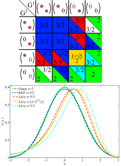
Figure 1: The scaling functions (bottom) and dynamical exponents are related to the structure of the mode coupling matrices $G^{\alpha}$ (top). The table shows the dynamical exponents $z_{\alpha}$ in the case $n=2$, see eq. (11). The symbols $\ast$ and $\star$ denote non-zero elements. Red symbols correspond to self-coupling, black symbols to couplings to other modes. Matrix elements not indicated can take any value. The colors in the table correspond to the colors of the graphs of the scaling functions.

III.2 Golden Mean case

As second representative example we consider the case where all self-coupling coefficients vanish, $G^{\alpha}_{\alpha\alpha}\equiv 0$ for all $\alpha$, while each mode has at least one nonzero coupling to another mode, $G^{\alpha}_{\beta\beta}\neq 0$ for some $\beta\neq\alpha$. Then, (5) reduces to $z_{\alpha}=1+1/z_{\beta}$ for all modes $\alpha,\ \beta$. The unique solution of this equation is the Golden Mean $z_{\alpha}=\varphi=(1+\sqrt{5})/2$ for all $\alpha$. The scaling functions (see Supporting Information section) are proportional to $\varphi$-stable Lévy distributions with parameters fixed by the collective velocities and the mode-coupling coefficients. The asymmetry of the fastest right-moving (left-moving) mode is predicted to be $\beta=-1$ ($\beta=1$).

IV Simulation results

To check the theoretical predictions for the two cases we simulate mass transport with three conservation laws, i.e., three distinct species of particles. To maintain a far-from-equilibrium situation a driving force is applied that leads to a constant drift superimposed on undirected diffusive motion. This is a natural setting for transport of charged particles in nanotubes, see Fig. 2 for an illustration, where a direct measurement of the stationary particle currents is experimentally possible Lee10 . However, due to the universal applicability of NLFH the actual details of the interaction of the particles with their environment and the driving field are irrelevant for the theoretical description of the large-scale dynamics. Hence for good statistics we simulate a lattice model for transport which represents a minimal realization of the essential ingredients, namely a non-linear current-density relation for all three conserved masses.

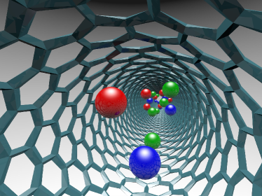
Figure 2: Schematic drawing of three particle species drifting inside a nanotube. Due to the interaction between the particles and with the walls one expects a non-linear current density relation.

Our model is the three-species version of the multi-lane totally asymmetric simple exclusion process Popk04 . Particles hop randomly in field direction on three lanes to their neighbouring sites on a periodic lattice of $3\times L$ sites with rates that depend on the nearest-neighbour sites. Lane changes are not allowed so that the total number of particles on each lane is conserved. Due to excluded-volume interaction each lattice site can be occupied by at most one particle. Thus the occupation numbers $n_{k}^{(\lambda)}$ of site $k$ on lane $\lambda$ take only values 0 or 1. The hopping rate $r_{k}^{(\lambda)}$ from site $k$ on lane $\lambda$ to site $k+1$ on the same lane is given by

$$r_{k}^{(\lambda)}=b_{\lambda}+\frac{1}{2}\sum_{\{\mu:\,\mu\neq\lambda\}}\gamma_{\lambda\mu}\left(n_{k}^{(\mu)}+n_{k+1}^{(\mu)}\right)$$ (7)

with a species dependent drift parameter $b_{\lambda}$ and symmetric interaction constants $\gamma_{\lambda\mu}=\gamma_{\mu\lambda}$. Hopping attempts onto occupied sites are rejected. The conserved quantities are the three total numbers of particles $N_{\lambda}$ on each lane with corresponding densities $\rho_{\lambda}=N_{\lambda}/L$.

The stationary distribution of our model factorizes Popk04 and thus allows for the exact computation of the macroscopic current-density relations $j_{\lambda}(\rho_{1},\rho_{2},\rho_{3})$ and the compressibility matrix $K(\rho_{1},\rho_{2},\rho_{3})$. Furthermore, because there is no particle exchange between lanes, the compressibility matrix is diagonal with elements denoted by $\kappa_{\lambda}$. One has

$$j_{\lambda} = \rho_{\lambda}(1-\rho_{\lambda})\left(b_{\lambda}+\sum_{\{\mu:\,\mu\neq\lambda\}}\gamma_{\lambda\mu}\rho_{\mu}\right)$$ (8)

$$\kappa_{\lambda} = \rho_{\lambda}(1-\rho_{\lambda}).$$ (9)

The diagonalization matrix $R$ and the mode-coupling matrices $G^{\alpha}$ are fully determined by these quantities.

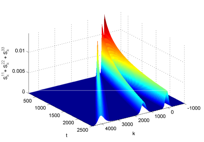
Figure 3: Space-time propagation of three normal modes in the three-lane model. The modes (from left to right) are the Fibonacci mode with $z=8/5$ (mode 3), the KPZ mode with $z=3/2$ (mode 1), and the Fibonacci mode with $z=5/3$ (mode 2). The physical and simulation parameters are given in the Appendices.

According to mode-coupling theory three different Fibonacci-modes with $z_{1}=3/2,z_{2}=5/3,z_{3}=8/5$ occur e.g. when $G^{1}_{11}\neq 0$, $G^{2}_{11}\neq 0$, $G^{3}_{22}\neq 0$, and $G^{2}_{22}=G^{2}_{33}=G^{3}_{33}=0$. For our simulation we compute numerically densities, bare hopping rates and interaction parameters to satisfy these properties as described in the Appendices. For this choice the velocities of the normal modes are $v_{1}=0.592315$, $v_{2}=0.0281578$, $v_{3}=1.58226$ which ensures a good spatial separation after quite small times. The propagation of the three normal modes (Fig. 3) with the predicted velocities is observed with an error of less than $10^{-3}$. Moreover, the numerically obtained dynamical structure function for mode $3$ shows a startling agreement with the theoretically predicted Lévy scaling function with $z=8/5$ and maximal asymmetry, see Fig. 4. It takes longer for the other two modes (KPZ mode and Lévy stable $5/3$ mode) to reach their asymptotic form, which we argue is due to the much smaller respective couplings, $(G^{1}_{11}/G^{3}_{22})^{2}\ll 1$, $(G^{2}_{11}/G^{3}_{22})^{2}\ll 1$.

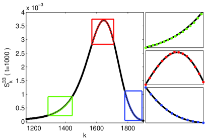
Figure 4: Left Panel: Vertical least squares fit of the numerically obtained dynamical structure function for the Fibonacci 8/5-mode (points), at time $t=1000$ with a 8/5-stable Lévy distribution, maximal asymmetry $-1$ and theoretical center of mass (line), predicted by the mode coupling theory. The only fit parameter is the scale parameter of the Lévy stable distribution. The simulation results agree very well with the asymptotic theoretical result already for moderate times. Right Panel: Insets show closeups of the peak region and tail regions, according to a colour code. Every $10$-th datapoint is plotted to improve the visibility of the data. The statistical error $\epsilon_{99\%}$ with 99% confidence bound is for every data point smaller than $1.6299\cdot 10^{-5}$.

In order to observe three Golden Mean modes it is sufficient to require that each mode has zero self-coupling and at least one nonzero coupling to other modes. This can be achieved with the set of parameters given in Appendices which lead to the velocities $v_{1}=1.83149$, $v_{2}=0.762688$, $v_{3}=0.326778$ of the normal modes. The propagation of the three normal modes with the predicted velocities is observed, approaching for large times a very small relative error of about $10^{-4}$. The structure function for the fastest mode $1$ converges to its asymptotic shape faster than for the other modes, due to the large coupling coefficient $G^{1}_{33}$. In Fig. 5 we show a scaling plot of the measured structure function for mode $1$ with dynamical exponent $z\equiv\varphi=\left(1+\sqrt{5}\right)/2$ together with a fitted to a $\varphi$-stable Lévy function (13) with maximal asymmetry $\beta=-1$ as predicted by the theory. The data collapse shows a striking agreement between the measured and theoretical scaling function. Alternatively, the dynamical exponent $z_{\alpha}$ can be derived from the maximum of the structure function, which scales as $\max(S_{1}(x,t))=\text{const}\cdot t^{-1/z}$. We obtain $z\approx 1.63$ which differs from the predicted value $z\equiv\varphi=(1+\sqrt{5})/2$ by less than $0.8\%$.

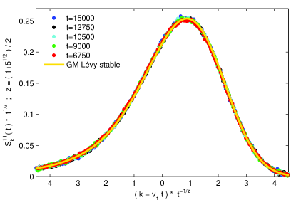
Figure 5: Scaling plot of the measured structure function of mode $1$ with dynamical exponent $z\equiv\varphi=\left(1+\sqrt{5}\right)/2$ for the Golden Mean case, fitted to a $\varphi$-stable Lévy distribution with maximal asymmetry $-1$ (see Eq. (13)). The scale parameter $E_{1}$ for the Lévy-stable distribution and the center of mass velocity $v_{1}$ are obtained by a vertical least square fit. Fitted parameters are $v_{1,\text{fit}}=1.83107\pm 0.00009$ and $E_{1,\text{fit}}=1.1\pm 0.01$. The fitted velocity $v_{1,\text{fit}}$ differs by $0.02\%$ from the theoretical velocity.

V Discussion

Our work demonstrates that non-equilibrium phenomena are much richer than just the diffusive and KPZ universality suggest. We have established that in non-equilibrium phenomena governed by non-linear fluctuating hydrodynamics with $n$ conservation laws mode coupling theory predicts a family of dynamical universality classes with dynamical exponents given by the sequence of consecutive Kepler ratios (6) of Fibonacci numbers. With slightly modified initial conditions on $G_{1}^{11}$ this result is easily generalized for the case when the first mode $\alpha=1$ is diffusive. Then the sequence of dynamical exponents becomes shifted by one unit with respect to (6). On the other hand, if all self-couplings vanish, but at least one other diagonal element $G^{\alpha}_{\beta\beta}$ of the mode coupling matrix is non-zero,one has as unique solution for all modes $\alpha$ the fixed point value $z_{\alpha}=z_{\infty}=\varphi$ which is the Golden Mean.

For general mode coupling matrices all critical exponents can be computed (from (11) in Appendices). The scaling functions of the non-diffusive and non-KPZ modes are asymmetric Lévy distributions whose parameters are completely determined by the macroscopic current-density relation and compressibility matrix of the system.

For 1+1 dimensional systems out of equilibrium this is the first time, to our knowledge, that an infinite family of discrete universality classes is found. Recalling that 1+1 dimensional non-equilibrium systems with short-range interactions can be mapped onto two-dimensional equilibrium systems (with the time evolution operator playing the role of the transfer matrix) one is reminded of the discrete families of conformally invariant critical equilibrium systems in two space dimensions Card96 ; Henk99 . We do not know whether there is any mathematical link, but the analogy is suggestive in so far as conformal invariance is a local symmetry of spatially isotropic systems with $z=1$ (which happens to be the lowest order Kepler ratio) while $z>1$ corresponds to strongly anisotropic systems for which also local symmetry groups are known to exist Henk02 .

Since an infinite number of lanes of coupled one-dimensional systems corresponds to a two-dimensional system, it is intriguing to observe that the Golden Mean is close to the numerical value $z=1.612-1.618$ of the dynamical exponent of the $2+1$-dimensional KPZ-equation Parisi ; HalpinHealy2 . The scaling function of the $2+1$-dimensional KPZ-equation, however, is not Lévy Scaling2dKPZ .

In order to observe and distinguish between the different new classes highly precise experimental data will be required. E.g. in the Fibonacci case the dynamical exponents converge quickly to the Golden Mean. A feature which might be easier to observe experimentally is the scaling function itself, which for higher Fibonacci ratios $5/3,8/5,...$ usually has a strong asymmetry (see Figs. 1, 4 and 5) while KPZ and Gauss scaling functions are symmetric. Growth processes which can be mapped on exclusion processes with several conservation laws, might be potentially suitable candidates for an experimental verification, see e.g. Take10 ; Take11 for an example of a system with one conservation law.

Appendix A Computation of the dynamical structure function

The mode coupling equations (4) can be solved in the scaling limit by applying a Fourier transform (FT) $f(x)\to\tilde{f}(p)$ and a Laplace transform (LT) $f(t)\to\tilde{f}(\omega)$. For more details we refer to Popk14b where the case $n=2$ of two conservation laws has been treated. After making the scaling ansatz

$$\tilde{S}_{\alpha}(p,\tilde{\omega}_{\alpha})=p^{-z_{\alpha}}g_{\alpha}(\zeta_{\alpha})$$ (10)

for the transformed dynamical structure function where $\hat{S}_{\alpha}(p,0)=1/\sqrt{2\pi}$ and $\zeta_{\alpha}=\tilde{\omega}_{\alpha}|p|^{-z_{\alpha}}$ we are in a position to analyze the small-$p$ behaviour. One has to search for dynamical exponents for which the limit $p\to 0$ is non-trivial, which requires a self-consistent treatment of all modes. We find that different conditions arise depending on which diagonal elements of the mode-coupling matrices vanish. To characterize the possible scenarios we define the set ${\mathbb{I}}_{\alpha}:=\{\beta:G^{\alpha}_{\beta\beta}\neq 0\}$ of non-zero diagonal mode coupling coefficients. Through power counting one obtains

$$z_{\alpha}=\left\{\begin{array}[]{lll}2&\mbox{ if }&{\mathbb{I}}_{\alpha}=\emptyset\\ 3/2&\mbox{ if }&\alpha\in{\mathbb{I}}_{\alpha}\\ \min_{\beta\in{\mathbb{I}}_{\alpha}}\left[\left(1+\frac{1}{z_{\beta}}\right)\right]&\mbox{ else }&\end{array}\right.$$ (11)

and the domain

$$1<z_{\alpha}\leq 2\quad\forall\alpha.$$ (12)

for the possible dynamical exponents.

In the Fibonacci case, the dynamical structure function of mode $\alpha$ in momentum space has the scaling form

$$\hat{S}_{\alpha}(p,t)=\frac{1}{\sqrt{2\pi}}\mathrm{e}^{-iv_{\alpha}pt-E_{\alpha}|p|^{z_{\alpha}}t\left(1-i\sigma_{p}^{\alpha\beta}\tan{\left(\frac{\pi z_{\alpha}}{2}\right)}\right)}$$ (13)

with inverse time scales $E_{\alpha}$. The dynamical exponents then satisfy the recursion (5). Up to the normalization $1/\sqrt{2\pi}$ the scaling form (13) is a $\alpha$-stable Lévy distribution Durrett .

Appendix B Simulation algorithm

For the Monte-Carlo simulation of the model we choose a large system size $L\geq 5\cdot 10^{5}$ which avoids finite-size effects. At time $t=0$, $N_{\lambda}$ particles are placed on each lane according to the desired initial state. One Monte-Carlo time unit consists of $3\cdot L\cdot r^{*}$ random sequential update steps where $r^{*}=\max\left\{{r_{k}}^{(\lambda)}\right\}$: In each update step a bond $(k^{(\lambda)},k^{(\lambda)}+1)$ is chosen randomly with uniform distribution. If $n_{k}^{(\lambda)}\left(1-n_{k+1}^{(\lambda)}\right)=1$ then the particle at site $k$ is moved to $k+1$ with probability $r_{k}^{(\lambda)}/r^{\ast}$ where $r^{\ast}$ is the maximal value that the $r_{k}^{(\lambda)}$ can take among all possible particle configurations on the neighbouring lanes. If $n_{k}^{(\lambda)}(1-n_{k+1}^{(\lambda)})=0$ the particle configuration remains unchanged.

Appendix C Simulation of the dynamical structure function

In order to determine the dynamical structure function we initialize the system by placing $N_{\lambda}$ particles uniformly on each lane $\lambda$. This yields a random initial distribution drawn from the stationary distribution of the process. No relaxation is required.

Then we use translation invariance and compute the space- and time average

$$\sigma_{L,k}^{\lambda\mu}(M,\tau,t)=\frac{1}{M}\sum_{j=1}^{M}\frac{1}{L}\sum_{l=1}^{L}n_{l+k}^{(\lambda)}(j\tau+t)n_{l}^{(\mu)}(j\tau)-\rho_{\lambda}\rho_{\mu}.$$ (14)

To avoid noisy data of $\sigma_{L,k}^{\lambda\mu}$ we take in (14) the system size $L$ and the time average parameter $M$ sufficiently large. In order to obtain $S_{k}^{\lambda\mu}(t)$ we average over $P$ independently generated and propagated initial configurations of $\sigma_{L,k}^{\lambda\mu}$. The error estimates for $S_{k}^{\lambda\mu}(t)$ are calculated from the $P$ independent measurements. From $S^{\lambda\mu}_{k}(t)$ we compute the structure function of the normal modes by transformation with the diagonalizing matrix $R$ determined by (8) and (9).

To obtain model parameters for three different Fibonacci-modes with $z_{1}=3/2,z_{2}=5/3,z_{3}=8/5$ we solve the equations given in the text after Eq. 9 numerically with a C-program performing direct minimization of the absolute values of the targeted G-elements until the given tolerance value ($10^{-6}$) is reached. The data shown here for the three mode case have been obtained from simulations with densities $\rho_{1}=0.2,\,\rho_{2}=0.25,\,\rho_{1}=0.3$, bare hopping rates $b_{1}=0.613185$, $b_{2}=0.425714$, $b_{3}=0.799831$ and interaction parameters $\gamma_{12}=1.36145$, $\gamma_{23}=3.69786$, $\gamma_{13}=0.143082$ for which the needed relations are satisfied. This choice of parameters yields $G^{1}_{11}=0.322507$, $G^{2}_{11}=-0.15$, $G^{3}_{22}=1.04547$, while the the absolute values of $G^{2}_{22},\,G^{2}_{33},\,G^{3}_{33}$ are smaller than $10^{-6}$. Besides these physical parameters, the simulation parameters for the Fibonacci modes (Fig. 3, 4) are $L=5\cdot 10^{5}$, $\tau=250$, $M=1400$, $P=98$.

For the Golden Mean case (Fig. 5) the set of parameters $\rho_{1}=0.2,\ \rho_{2}=\rho_{3}=0.25$, $\gamma_{12}=0.0082334758646$, $\gamma_{23}=1.68447706968$, $\gamma_{13}=3.72140740146$, and $b_{1}=0.905073261248$, $b_{2}=0.86$, and $b_{3}=1.18875738638$. This leads to $G^{1}_{22}=0.405702$, $G^{1}_{33}=0.929315$, $G^{2}_{11}=-0.104141$, $G^{2}_{33}=-0.208477$, $G^{3}_{11}=-0.182467$, $G^{3}_{22}=0.271246$, while the absolute values of $G^{1}_{11},G^{2}_{22},G^{3}_{33}$ are smaller than $10^{-6}$. The simulation parameters for the Golden Mean case are $L=5\cdot 10^{6}$, $\tau=750$, $M=30$ and $P=303$.

Supporting Information

Remarkably, the mode coupling equations eq. (4) can be solved exactly in the scaling limit by Fourier and Laplace transformation. To this end we define the Fourier transform (FT) as

$$\hat{f}(p):=\frac{1}{\sqrt{2\pi}}\int_{-\infty}^{\infty}\mathrm{d}x\,\mathrm{e}^{-ipx}f(x),$$ (15)

and the Laplace transform (LT) as

$$\tilde{f}(\omega):=\int_{0}^{\infty}\mathrm{d}t\,\mathrm{e}^{-\omega t}f(t).$$ (16)

With $\widehat{D}_{\alpha}(p)=iv_{\alpha}p+D_{\alpha}p^{2}$ we obtain from eq. (4) of the paper in momentum-frequency space

$$\tilde{S}_{\alpha}(p,\omega)=\frac{\hat{S}_{\alpha}(p,0)}{\omega+\widehat{D}_{\alpha}(p)+\tilde{C}_{\alpha\alpha}(p,\omega)}$$ (17)

with memory kernel

$$\tilde{C}_{\alpha\alpha}(p,\omega)=2\sum_{\beta,\gamma}(G^{\alpha}_{\beta\gamma})^{2}p^{2}\int_{0}^{\infty}\mathrm{d}s\,\mathrm{e}^{-\omega s}\int_{{\mathbb{R}}}\mathrm{d}q\hat{S}_{\beta}(q,s)\hat{S}_{\gamma}(p-q,s).$$ (18)

and $\hat{S}_{\alpha}(p,0)=1/\sqrt{2\pi}$.

Next we introduce $\tilde{\omega}_{\alpha}:=\omega+iv_{\alpha}p$ and make the scaling ansatz

$$\tilde{S}_{\alpha}(p,\tilde{\omega}_{\alpha})=p^{-z_{\alpha}}g_{\alpha}(\zeta_{\alpha})$$ (19)

with $\zeta_{\alpha}=\tilde{\omega}_{\alpha}|p|^{-z_{\alpha}}$. Having in mind systems with short-range interactions we anticipate that all modes spread subballistically, i.e., $z_{\alpha}>1$ for all $\alpha$. Using strict hyperbolicity one obtains after some substitutions of variables

$$g_{\alpha}(\zeta_{\alpha}) = \lim_{p\to 0}\left[\zeta_{\alpha}+D_{\alpha}|p|^{2-z_{\alpha}}+Q_{\alpha\alpha}\zeta_{\alpha}^{2-z_{\alpha}-\frac{1}{z_{\alpha}}}|p|^{3-2z_{\alpha}}\right.$$ (20)

$$+ \left.\sum_{\beta\neq\alpha}Q_{\alpha\beta}\left(-iv_{p}^{\alpha\beta}\right)^{\frac{1}{z_{\beta}}-1}|p|^{1+\frac{1}{z_{\beta}}-z_{\alpha}}\right]^{-1}.$$

with $v_{p}^{\alpha\beta}:=|v_{\alpha}-v_{\beta}|\mathrm{sgn}[p(v_{\alpha}-v_{\beta})]$ and

$$Q_{\alpha\beta}=2(G^{\alpha}_{\beta\beta})^{2}\Gamma\left(1-\frac{1}{z_{\beta}}\right)\Omega[\hat{S}_{\beta}]\geq 0.$$ (21)

where

$$\Omega[\hat{f}]=\int_{-\infty}^{\infty}\mathrm{d}p\,\hat{f}(p)\hat{f}(-p).$$ (22)

With $\sigma_{p}^{\alpha\beta}=\mathrm{sgn}[p(v_{\alpha}-v_{\beta})]$ one has

$$\left(-iv_{p}^{\alpha\beta}\right)^{\frac{1}{z_{\beta}}-1}=\sin{\left(\frac{\pi}{2z_{\beta}}\right)}|v_{\alpha}-v_{\beta}|^{\frac{1}{z_{\beta}}-1}\times$$

$$\left[1-i\sigma_{p}^{\alpha\beta}\tan{\left(\left(1+\frac{1}{z_{\beta}}\right)\frac{\pi}{2}\right)}\right].$$ (23)

Now we are in a position to analyze the small-$p$ behaviour. One has to search for dynamical exponents for which the limit $p\to 0$ is non-trivial, which is determined by the smallest power of $p$ in (20). This has to be done self-consistently for all modes. We find that different conditions arise depending on which diagonal elements of the mode-coupling matrices vanish. In order to characterize the possible scenarios we define the set ${\mathbb{I}}_{\alpha}:=\{\beta:G^{\alpha}_{\beta\beta}\neq 0\}$ of non-zero diagonal mode coupling coefficients. One obtains from (20) through power counting the system of equations

$$z_{\alpha}=\left\{\begin{array}[]{lll}2&\mbox{ if }&{\mathbb{I}}_{\alpha}=\emptyset\\ 3/2&\mbox{ if }&\alpha\in{\mathbb{I}}_{\alpha}\\ \min_{\beta\in{\mathbb{I}}_{\alpha}}\left[\left(1+\frac{1}{z_{\beta}}\right)\right]&\mbox{ else }&\end{array}\right.$$ (24)

and the domain

$$1<z_{\alpha}\leq 2\quad\forall\alpha.$$ (25)

for the possible dynamical exponents.

- (1) Livio M (2003) The Golden Ratio: The Story of PHI, the World’s Most Astonishing Number, Broadway Books (ISBN 978076790815).
- (2) Landi GT, de Oliveira MJ (2014) Fourier’s law from a chain of coupled planar harmonic oscillators under energy-conserving noise. Phys. Rev. E 89(2): 022105.
- (3) Gendelman OV, Savin AV (2014) Normal heat conductivity in chains capable of dissociation. EPL 106: 34004.
- (4) Kardar M, Parisi G, Zhang Y-C (1986) Dynamic scaling of growing interfaces. Phys. Rev. Lett. 56: 889–892.
- (5) Spohn H (2014) Nonlinear Fluctuating hydrodynamics for anharmonic chains. J. Stat. Phys. 154: 1191–1227.
- (6) Spohn H (2015) Fluctuating hydrodynamics approach to equilibrium time correlations for anharmonic chains. arXiv:1505.05987.
- (7) Maunuksela J, Myllys M, Kähkönen O-P, Timonen J, Provatas N, Alava MJ, Ala-Nissila T (1997) Kinetic roughening in slow combustion of paper. Phys. Rev. Lett. 79: 1515.
- (8) Miettinen L, Myllys M, Merikoski J, Timonen J (2005) Experimental determination of KPZ height-fluctuation distributions. Eur. Phys. J. B 46: 55–60.
- (9) Wakita J, Itoh H, Matsuyama T, Matsushita M (1997) Self-affinity for the growing interface of bacterial colonies, J. Phys. Soc. Jpn. 66(1): 6772.
- (10) Yunker PJ, Lohr MA, Still T, Borodin A, Durian DJ, Yodh AG (2013) Effects of particle shape on growth dynamics at edges of evaporating drops of colloidal suspensions. Phys. Rev. Lett. 110: 035501.
- (11) For a nice introduction into the KPZ class and its relevance we refer to Buchanan14 . Recent reviews HalpinHealy ; QuastelSpohn provide a more detailed account of theoretical and experimental work on the KPZ class.
- (12) Buchanan M (2014) Equivalence principle. Nature Physics 10(8): 543.
- (13) Halpin-Healy T, Takeuchi K.A. (2015) A KPZ cocktail - shaken, not stirred: toasting 30 years of kinetically roughened surfaces. J. Stat. Phys. 160: 794.
- (14) Quastel J, Spohn H (2015) The one-dimensional KPZ equation and its universality class. J. Stat. Phys. 160: 965.
- (15) Prähofer M, Spohn H (2004) Exact scaling functions for one-dimensional stationary KPZ growth. J. Stat. Phys. 115: 255–279.
- (16) Prähofer M, Spohn H (2002) Current fluctuations in the totally asymmetric simple exclusion process. In and Out of Equilibrium, Vol. 51 of Progress in Probability, ed. Sidoravicius V (Birkhauser, Boston).
- (17) Takeuchi KA, Sano M (2010) Universal fluctuations of growing interfaces: evidence in turbulent liquid crystals. Phys. Rev. Lett. 104: 230601.
- (18) Takeuchi KA, Sano M, Sasamoto T, Spohn H (2011) Growing interfaces uncover universal fluctuations behind scale invariance. Sci. Rep. 1: 34.
- (19) Van Beijeren H (2012) Exact results for anomalous transport in one-dimensional Hamiltonian systems. Phys. Rev. Lett. 108: 108601.
- (20) Mendl CB, Spohn H (2013) Dynamic correlators of FPU chains and nonlinear fluctuating hydrodynamics. Phys. Rev. Lett. 111: 230601.
- (21) Spohn H, Stoltz G (2015) Nonlinear fluctuating hydrodynamics in one dimension: The case of two conserved fields. J. Stat. Phys. 160: 861.
- (22) Popkov V, Schmidt J, Schütz GM (2014) Superdiffusive modes in two-species driven diffusive systems. Phys. Rev. Lett. 112: 200602.
- (23) Popkov V, Schmidt J, Schütz GM (2015) Universality classes in two-component driven diffusive systems. J. Stat. Phys. 160: 835–860.
- (24) Grisi R, Schütz GM (2011) Current symmetries for particle systems with several conservation laws. J. Stat. Phys. 145: 1499–1512.
- (25) Tóth B, Valkó B (2003) Onsager relations and Eulerian hydrodynamic limit for systems with several conservation laws. J. Stat. Phys. 112: 497–521.
- (26) Devillard P, Spohn H (1992) Universality class of interface growth with reflection symmetry. J. Stat. Phys. 66: 1089–1099.
- (27) Durrett R (2010) Probability: Theory and Examples (4th Edition), Cambridge University Press, Cambridge, p. 141.
- (28) Lee CH, Choi W, Han J-H, Strano MS (2010) Coherence resonance in a single-walled carbon nanotube ion channel. Science 329: 1320–1324.
- (29) Popkov V, Salerno M (2004) Hydrodynamic limit of multichain driven diffusive models. Phys. Rev. E 69: 046103.
- (30) Cardy J (1996) Scaling and Renormalization in Statistical Physics (Cambridge University Press, Cambridge)
- (31) Henkel M (1999) Conformal Invariance and Critical Phenomena (Springer, Berlin).
- (32) Henkel M (2002) Phenomenology of local scale invariance: From conformal invariance to dynamical scaling. Nucl. Phys. B 641: 405–486.
- (33) Pagnani A, Parisi G (2015) Numerical estimate of the Kardar-Parisi-Zhang universality class in (2+1) dimensions. Phys. Rev. E 92, 010101
- (34) Halpin-Healy, T (2012) (2+1)-dimensional directed Polymer in a random medium: scaling phenomena and universal distributions. Phys. Rev. Lett. 109, 170602
- (35) Kloss T, Canet L, Wschebor N (2012) Nonperturbative renormalization group for the stationary Kardar-Parisi-Zhang equation: Scaling functions and amplitude ratios in 1+1, 2+1, and 3+1 dimensions. Phys. Rev. E86, 051124