Spin Excitations and Correlations in Scanning Tunneling Spectroscopy

Abstract

In recent years inelastic spin-flip spectroscopy using a low-temperature scanning tunneling microscope has been a very successful tool for studying not only individual spins but also complex coupled systems. When these systems interact with the electrons of the supporting substrate correlated many-particle states can emerge, making them ideal prototypical quantum systems. The spin systems, which can be constructed by arranging individual atoms on appropriate surfaces or embedded in synthesized molecular structures, can reveal very rich spectral features. Up to now the spectral complexity has only been partly described. This manuscript shows that perturbation theory enables one to describe the tunneling transport, reproducing the differential conductance with surprisingly high accuracy. Well established scattering models, which include Kondo-like spin-spin and potential interactions, are expanded to enable calculation of arbitrary complex spin systems in reasonable time scale and the extraction of important physical properties. The emergence of correlations between spins and, in particular, between the localized spins and the supporting bath electrons are discussed and related to experimentally tunable parameters. These results might stimulate new experiments by providing experimentalists with an easily applicable modeling tool.

1 Introduction:

With low-temperature scanning tunneling microscopes (STM) scientist have developed a tool that has the ability to detect and manipulate individual magnetic spin systems on the atomic and molecular level by an externally controlled probe with sub-nm precision. These instruments have opened a new field of research envisioning not only a deeper understanding of the origin of molecular magnetism by studying the interactions between nanoscale spins but also of the many-particle effects between the localized spins and the itinerant electrons of the supporting substrate. The progress in this field is best demonstrated by the recently achieved ability to build stable magnetic bits by cleverly arranging only a handful of Fe atoms on either a thin insulating [1] or on a nonmagnetic Cu(111) surface [2]. While in these experiments the transition from quantum-mechanical to classical magnetic behavior is explored [3], other applications might be envisioned ranging from spin-based logic circuits [4] to entangled systems in which the quantum mechanical nature is crucial for computational purposes [5].

At the basis of all these experiments lies the spectroscopic capability of the STM. About ten years ago A. Heinrich and his co-workers showed in a hallmark experiment that it is possible to detect inelastic spin-flip excitations on Mn atoms adsorbed on patches of Al₂O₃ on a NiAl surface [6]. Since then many experiments have focused on transition metal atoms on a thin layer of Cu₂N on Cu(100) [7, 8, 9, 10, 11, 12, 13, 14, 1, 15, 16, 17, 18, 19, 20]. In these experiments, patches of Cu₂N are formed by sputtering a clean Cu(100) surface with N⁺ ions and subsequent annealing. This leads to a monolayer of Cu₂N on the surface on which the desired metal atoms are deposited (Figure 1a). Experimentally, every 3d transition metal atom adsorbed on this surface reveals its fingerprint when a spectrum is taken by placing the tunneling tip of an STM over the atom (Figure 1b). The spectra are measured by varying the bias voltage applied between tip and sample and recording the differential conductance $dI/dV$. All spectra show characteristic features that can be classified into two groups: (1) Step-like increases in the differential conductance, positioned symmetrically around zero bias, and (2) peaks of the differential conductance at zero bias.

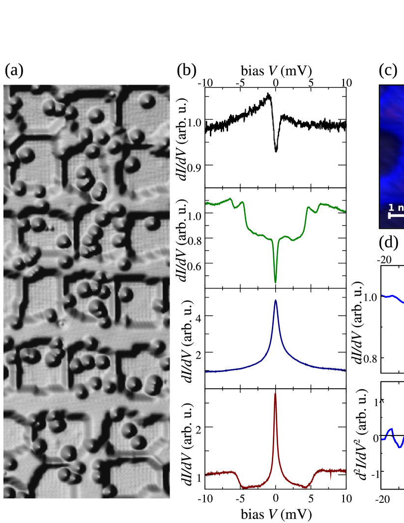
Figure 1: Some examples of inelastic spin-flip spectroscopy on single atoms and molecules. (a) Constant current topography of the Cu₂N surface on Cu(100) with co-adsorbed 3d metal atoms. (size approx.: $15\times 40$ nm², $V=10$ mV, $I=1$ nA). (b) Differential conductance $dI/dV$ spectra measured on top of Mn, Fe, Ti, and Co adatoms (from top to bottom) at zero magnetic field and $T=0.6$ K. Each atom reveals a characteristic fingerprint in the $dI/dV$ signal. (c) Constant current topography of a Mn₁₂Ac₁₆ molecular magnet adsorbed on $h$-BN on Rh(111) ($V=-1$ V, $I=45$ pA). (d) Typical $dI/dV$ and $d^{2}I/dV^{2}$ spectra at $T=1.5$ K and zero magnetic field on Mn₁₂Ac₁₆. (e) Constant current topography of an organic radical molecule (C₂₈H₂₅O₂N₄) adsorbed on Au(111) ($V=100$ mV, $I=33$ pA, Contour line distances 50 pm).(f) $dI/dV$ spectra at different temperatures ($T=1.5,\ 3,\ 4.4,\ 6.7$ K, bottom to top, upper panel) and magnetic fields ($B=14,\ 10,\ 6,\ 2$ T, bottom to top, lower panel) on the radical. Spectra are vertically offset for clarity. Data adapted from [9, 8, 21, 22].

The number of distinguishable conductance steps varies for different spin systems and the precise form of the steps often shows some asymmetry with respect to the applied bias direction and can exhibit some overshoot of the conductance at the step-energy. As we will see in detail, the steps are due to the opening of additional conductance channels precisely governed by the magnetic properties of the spin system. These excitations can be present even at zero magnetic field due to the magneto-crystalline anisotropy. The anisotropy is caused by the reduction of the geometric symmetry at the surface and by spin-orbit coupling [23, 24, 25], which have the effect of lifting the inherent degeneracy of the spin states. For single atoms the maximum anisotropy is limited to a few tens of meV [26], whereby the magnetic excitation energies usually range from less than one meV up to a few meV requiring experimental setups operating at temperatures $T\leq 4$ K. Here, it is worth to note that one has to be aware that not all energetically low lying step-like increases in the differential conductance must originate from magnetic excitations. The tunneling electrons can also excite low-energy mechanical vibrations which can produce similar strong spectroscopic features [27, 28, 29, 30, 12, 31] and which can interact with the spin excitations [32, 33]. Thus, to clearly distinguish magnetic excitations their behavior in external applied magnetic fields is often crucial.

The peaks at zero bias are due to the Kondo effect in which itinerant electrons from the substrate coherently scatter with the localized magnetic moment of the adatom [34, 35, 36]. This effect has first been detected by scanning tunneling spectroscopy on single metal atoms adsorbed on noble metal substrates [37, 38, 39, 40, 41, 42, 43, 44, 45, 46]. In these early experiments the metal atoms are relatively strongly coupled to the substrate leading to a characteristic Kondo temperature in the range of $T_{K}\approx 30-300$ K, as determined by the full-width at half-maximum of the peak, and in most cases to a strongly asymmetric Fano lineshape due to interference effects with a potential scattering channel [47, 48, 49]. A decoupling layer, such as Cu₂N, significantly reduces the Kondo temperature suggesting the possibility of influencing this many-body state with experimentally accessible magnetic fields and temperatures [9, 50, 18, 51]. This enables the study of the interplay between Kondo screening, the magnetic anisotropy, and nearby spins [10, 20].

Apart from Cu₂N, other decoupling substrates have been exploited to study spin excitations. For example, low-lying excitations associated with a spin $S=1$ of the magnetic atom have been found for single Fe atoms embedded into the semiconducting InSb(110) surface [52, 53], which exhibits a two-dimensional electron gas confined to the surface. Other experiments used two-dimensional materials, such as graphene and hexagonal boron nitride ($h$-BN), as substrates for metal adatoms or magnetic molecules. For example, the Kondo state was observed for individual Co atoms adsorbed on a graphene sheet on top of a Ru(0001) surface with different Kondo temperatures and effective $g$-factors depending on the adsorption site with respect to the underlying metal [50]. In a different experiment Co and CoH_x ($x=1-3$) complexes on graphene on top of Pt(111) have been investigated revealing a $S=1$ for Co and CoH₃ and a high magnetic anisotropy of $\approx 8.1$ meV for the Co adsorbate [54]. On the highly corrugated and insulating $h$-BN adlayer on top of a Rh(111) substrate, CoH and CoH₂ complexes showed both, spin-flip excitations and the Kondo effect, pointing to two different spin states of $S=1$ and $S=1/2$, respectively [51]. Interestingly, the CoH complex revealed a dependence of the effective anisotropy on the coupling to the underlying substrate, similarly as observed for Co atoms on large patches of Cu₂N [16].

Spin excitations can also be observed for spin systems adsorbed on bare metal substrates, even though lifetime, anisotropy energies, and intensities are in general reduced due to the strong coupling with the substrate. For example, spin-excitations of Co and Fe on Pt(111) have been measured [55, 56], where the measurements of reference [55] were performed at $T\approx 6$ K and showed an approximately ten-times higher apparent magnetic anisotropy as the latter measurement (reference [56]) that was performed at $T=0.3$ K. This discrepancy stems from the strong temperature dependent broadening of the spectrum, which leads to this gross overestimation and illustrates the need for low-temperature measurements [57]. Additionally, spin excitations have been detected for Fe atoms adsorbed on Cu(111) [58] and on Ag(111) [59]. Apart from the 3d transition metal atoms, 4f lanthanide atoms also show low-energy magnetic signals. For example, the Kondo effect was measured on small Ce clusters on Cu₂N [12] and spin-flip signals were observed for Gd adsorbed on Pt(111) and Cu(111) [60] and Ho on Pt(111) [61], even though the intensities of the spin-flip excitations are unclear but presumably very small due to the strong localization of the 4f wavefunctions close to the nuclei and their small spacial extension [62].

In addition to these, metal-organic complexes, such as $M$-phthalocyanine with $M=$ Mn, Fe, Co, Ni, and Cu, have been studied on different surfaces [63, 64, 65, 66, 67, 68, 69, 70]. Many of them showed Kondo screening with a lower Kondo temperature enabling the tuning by dehydrogenation [63, 70] or the splitting of the peak by an externally applied magnetic field [64, 68] or by coupling to a ferromagnetic substrate [71]. Interestingly, FePc adsorbed on Au(111) showed a clear Kondo signature [69], while the same molecule adsorbed on top of a CuO decoupling layer showed a double-step in the differential conductance pointing to $S=1$ [65].

The electronic decoupling can also be created by using a substrate in the superconducting state in which the creation of Cooper pairs leads to a strongly reduced density of unpaired electrons around the Fermi energy. This results in a significant increase of the spin lifetime of the metal-organic complex [72]. Furthermore, such a substrate allows one to study the competition between superconducting phenomena and Kondo screening as observed on MnPc adsorbed on Pb(111) [67, 73].

Apart from metal atoms and metal-organic complexes spin-flip excitations were detected in complex molecules in which several spin centers are coupled forming a giant spin, as it has been shown at the example of the prototypical molecular magnet manganese-12-acetate-16 which has a ground state with a total spin of $S=10$ [21] (Figure 1c and d). Here, the $h$-BN decoupling layer is crucial as the magnetism is strongly quenched when the molecule is adsorbed upon a Au(111) surface. Furthermore, fully organic molecules including the charge-transfer complexes TTF-TCNQ (tetrathiafulvalene-tetracyanoquinodimethane) [32] and an organic radical molecule [22], have shown the Kondo effect, whereby for the latter molecule the temperature and magnetic field dependence was fully understood and simulated in a perturbative approach (figure 1e and f).

To describe the inelastic spin-flip excitation spectra, scattering models have been developed that treat the interaction of the tunneling electron with the localized spin system effectively as a one-electron second-order perturbation [74, 75, 76, 77]. Additionally, similar models allowed rationalization of the change in the spectra when a spin-polarized tip is employed [78] and the dynamics at increased coupling between tip and sample [79, 80, 81]. To address the experimentally observed bias asymmetry, co-tunneling models in the strong Coulomb-blockade regime have been proposed [82] and many-electron effects using the non-crossing approximation have been included [83]. Furthermore, third-order scattering models similar to the ones used here were employed to well describe the observed bias overshooting at certain inelastic excitation steps [84, 85]. Nevertheless, these models were restricted to Kondo-like interactions and did not include potential scattering.

In this paper, I plan to review the straightforward model of the exchange-interaction between an isolated spin system and the tunneling electrons and use a perturbative tunneling approach to simulate experimental data with unprecedented accuracy. The basic idea of the model goes back 50 years to the hallmark discovery of Juan Kondo that higher order scattering of bulk electrons on a magnetic impurity leads to logarithmic divergences [34, 35]. We will see that such a model enables the determination of physical properties like the magnetocrystalline anisotropy, the coupling strength to the substrate, the state lifetimes, and the magnetization directly by comparing the differential conductance measurements with simulations. Furthermore, it allows one to grasp some of the correlations and entanglements that are formed by the many-particle interactions due to the large electron bath of the substrate. The model, even though inherently limited due to its perturbative approach, has the advantage that we can develop it straightforwardly using simple matrix algebra. Due to this simplicity it is computationally very fast and can thus help us to understand future experimental observations. In these calculations the magnetic anisotropies, gyromagnetic factors, and coupling strengths to the substrate enter as experimentally determined parameters. Note however, that in particular for transition metal atoms adsorbed on metallic substrates the magnetic anisotropy have been successfully determined from first principle by, for example, time-dependent density functional theory [86, 87, 56, 88] or density functional theory which includes spin-orbit coupling [89, 90].

The basic idea of the model is to treat the tunneling as a scattering event of an incoming electron with the localized spin system (Figure 2a). Postponing the exact meaning for later, it is amazing that only two parameters govern these interactions: The Kondo scattering parameter $J$ and the potential scattering parameter $U$. These two parameters are crucial for the understanding of the low-energy excitations. One is tempted to ask “What is the origin of these?” To find an answer it is helpful to step back from the scattering picture and look at the single-impurity Anderson model, which describes one half-filled atomic orbital (for example from a 3d transition metal atom) interacting with the continuous states of a host metal (Figure 2b) [91]. In this picture all energies are in the eV range and it is not per se clear how this relates to the scattering model with low-energy excitations in the meV range. These relations were found by Schrieffer and Wolf, who were able to relate the high energies of the Anderson model with the scattering parameters [92]:

$$J=\frac{2}{\pi}\Delta^{2}\left(\frac{1}{\epsilon_{d}}-\frac{1}{\epsilon_{d}+U_{d}}\right)<0,\quad\quad\mathcal{U}=\frac{2}{\pi}\Delta^{2}\left(\frac{1}{\epsilon_{d}}+\frac{1}{\epsilon_{d}+U_{d}}\right).$$ (1)

Here it is crucial for the understanding of the forthcoming model that the Kondo spin-spin exchange scattering $J$ is for $S=1/2$ systems always negative, which means that the localized spin and the substrate electrons couple antiferromagnetically, while the potential scattering $\mathcal{U}$ can have both signs, either positive or negative. However, this result can be different for higher spins.

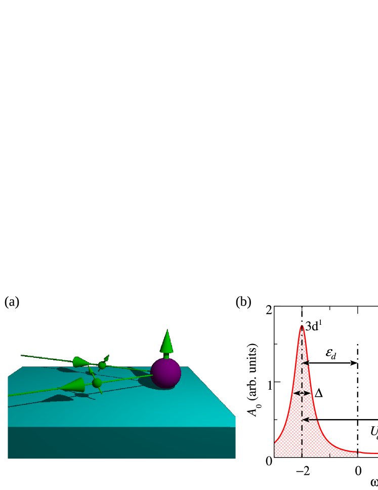
Figure 2: Comparison of the Kondo scattering and the single-impurity Anderson model. (a) Schematic view of the Kondo model where electrons scatter via spin-flip or the potential interaction with a localized spin system. (b) Schematic view of the single orbital Anderson impurity model. An occupied 3d orbital located at an energy $\varepsilon_{d}$ below the Fermi energy hybridize with the substrate electrons leading to a state broadening $\Delta$. The occupation of this orbital with a second electron is prohibited by the Coulomb repulsion energy $U_{d}$.

The manuscript is organized as follows: In section 2 the basic model in the zero-current approximation is introduced and discussed for the example spin $S=1/2$. In section 3 high-spin systems are discussed. Experimentally observed examples are given and compared to the model calculations. Section 4 discusses the limitations of the model, in particular, its inability to cover all correlation effects that occur when a system enters the strong Kondo regime using experimental data obtained on the Co/Cu₂N system as an example. In section 5 the initial model is extended by including rate equations and tested against experimental data. Here, we will observe that the tunneling current too can lead to the appearance of a non-equilibrium Kondo effect. Finally, section 6 summarizes the manuscript and outlines possible routes for future extensions.

2 The model

To describe the experimental observations we use a simplified model in which the Hamiltonian of the total quantum mechanical system is divided into the ones of the subsystems of the two electron reservoirs in tip and sample, the one of the localized spin system, and an interaction Hamiltonian that enables the exchange of charge carriers between the reservoirs:

$$\hat{H}=\hat{H}_{t}+\hat{H}_{s}+\hat{H}_{a}+\hat{H}^{\prime}$$ (2)

The Hamiltonian of the tip $\hat{H}_{t}$ and sample $\hat{H}_{s}$, respectively, can be described in the framework of second quantization using creation and annihilation operators $\hat{a}^{\dagger}$ and $\hat{a}$:

$$\hat{H}_{t}=\sum_{k,\sigma}\epsilon_{{\rm t}k\sigma}\hat{a}^{\dagger}_{{\rm t}k\sigma}\hat{a}_{{\rm t}k\sigma},$$ (3)

$$\hat{H}_{s}=\sum_{k,\sigma}\epsilon_{{\rm s}k\sigma}\hat{a}^{\dagger}_{{\rm s}k\sigma}\hat{a}_{{\rm s}k\sigma},$$ (4)

with $\epsilon_{{\rm t}k\sigma}$ and $\epsilon_{{\rm s}k\sigma}$ as the energy of the electrons with momentum $k$ and spin $\sigma$ in the tip and sample, respectively.

These two many-particle systems are the source and sink for the tunneling electrons in the STM experiment. Instead of using creation and annihilation operators in the momentum space $k$, we assume in the small energy range of interest, i. e. to some tens of meV around the Fermi energy, for tip and sample a continuous and energetically flat density of states $\rho(\epsilon)=\sum_{\sigma,k(\epsilon),k^{\prime}(\epsilon)}\delta_{k,k^{\prime}}\left\langle\hat{a}^{\dagger}_{k\sigma}\hat{a}_{k^{\prime}\sigma}\right\rangle\equiv\rho$, with $\left\langle\cdot\right\rangle$ as the time averaged expectation value.

In general, the electronic states $|\varphi\rangle$ in these electrodes might be spin-polarized in an arbitrary direction which we account for by the corresponding spin density matrices $\varrho=|\varphi\rangle\langle\varphi|=\frac{1}{2}(\hat{I}+\vec{n}\cdot\hat{\bm{\sigma}})$. Here, $\vec{n}$ describes the direction and $-1\leq|\vec{n}|\leq 1$ the amplitude of the polarization in the chosen coordinate system, $\hat{\bm{\sigma}}=(\hat{\sigma}_{x},\hat{\sigma}_{y},\hat{\sigma}_{z})$ are the standard Pauli matrices, and $\hat{I}$ is the $(2\times 2)$ identity matrix. With this convention the spin polarization is identical to the relative imbalance between majority and minority spin densities $\eta=|\vec{n}|=\left|\frac{\rho_{\uparrow}-\rho_{\downarrow}}{\rho_{\uparrow}+\rho_{\downarrow}}\right|$ where $\uparrow$ and $\downarrow$ account for the two different spin directions along the chosen quantization axis. This description via density matrices allows arbitrary polarization directions in tip and sample which obey the quantum statistics (see A).

The impurity spin system may either contain only a single spin or a finite number of coupled spins. We describe this system by a model Hamiltonian $\hat{H}_{a}$ that includes Zeeman and magnetic anisotropy energy and – in the case of more than one spin – the Heisenberg coupling terms $\vec{\mathcal{J}}_{ij}$ and the non-collinear Dzyaloshinskii-Moriya coupling $\vec{\mathcal{D}}_{ij}$ between individual spins:

$$\hat{H}_{a}=\sum_{i}g_{i}\mu_{B}\vec{B}\cdot\hat{\bf S}^{i}+\sum_{i}\left(D_{i}(\hat{S}_{z}^{i})^{2}+E_{i}\left[(\hat{S}_{x}^{i})^{2}-(\hat{S}_{y}^{i})^{2}\right]\right)$$

$$+\sum_{i,j}\vec{\mathcal{J}}_{ij}\hat{\bf S}^{i}\cdot\hat{\bf S}^{j}+\sum_{i,j}\vec{\mathcal{D}}_{ij}\hat{\bf S}^{i}\times\hat{\bf S}^{j}.$$ (5)

In this equation $\mu_{B}$ is the Bohr magneton and $g_{i}$, $D_{i}$, and $E_{i}$ are the gyromagnetic factor, the axial and the transversal magnetic anisotropy for the $i$-th spin in the reference coordinate frame, respectively. The externally applied magnetic field is $\vec{B}$ and the total spin operators $\hat{\bf S}^{i}=(\hat{S}_{x}^{i},\hat{S}_{y}^{i},\hat{S}_{z}^{i})$ are built from operators of the form $\hat{S}^{i}_{x,y,z}=\hat{I}_{1}\otimes\cdots\otimes\hat{S}_{x,y,z}^{i}\otimes\cdots\otimes\hat{I}_{n}$, which only act on the $i$-th spin and where $\hat{I}$ denotes the identity matrix and $\otimes$ the Kronecker matrix product. The spin operators $\hat{S}_{x,y,z}^{i}$ can be easily constructed remembering that $\hat{S}_{z}|\psi_{m}\rangle=\hbar m_{z}|\psi_{m}\rangle$ with $m_{z}=S,S-1,\cdots,-S$ as the magnetic quantum number along our chosen $z$-axis and $\hat{S}_{\pm}|\psi_{m}\rangle=\hbar\sqrt{(S\mp m)(m\pm S+1)}|\psi_{m\pm 1}\rangle$. These then enable calculation of $\hat{S}_{x}=\frac{1}{2}(\hat{S}_{+}+\hat{S}_{-})$ and $\hat{S}_{y}=-\frac{1}{2}i(\hat{S}_{+}-\hat{S}_{-})$, respectively. For simplicity we will set $\hbar=1$ from now on.

Diagonalizing the Hamiltonian of the localized spin system (equation 5) leads to discrete energy eigenvalues $\epsilon_{n}$ and eigenstates $|\psi\rangle_{n}$. For a single spin there are $2S+1$ eigenstates, while for complex spin structures that consist of several spins the number of eigenstates increases quickly as $\prod_{i}(2S_{i}+1)$. Because we neglect direct interactions between the electron baths in tip, sample and the localized spin system, we describe the total state as a product of the continuous electron states $|\varphi\rangle$ and the discrete spin states $|\psi\rangle$, i. e. $|\varphi^{\rm t,s},\psi\rangle=|\varphi^{\rm t,s}\rangle|\psi\rangle$. Note, however, that the coupling of the spin-system with the substrate will lead to an entanglement between sample electrons and the spin system (see section 4) and to a renormalization of the parameters in equation 5 [93, 16, 94, 51]. Here we assume that the renormalization is already included in the anisotropies and gyromagnetic factors and omit for the moment the entanglement.

The interaction Hamiltonian $H^{\prime}$ of equation 2 allows for tunneling of electrons from tip to sample or vice versa only via Kondo-like spin-flip or potential scattering processes with the impurity (Figure 3a):

$$\hat{H}^{\prime}=\hat{V}_{\rm t\rightarrow s}+\hat{V}_{\rm s\rightarrow t}+\hat{V}_{\rm s\rightarrow s},$$

$$\hat{V}_{\rm t\rightarrow s}=\sum_{i,\lambda^{\prime},\lambda}T_{ta}^{i}J_{i}\,\hat{a}_{{\rm s}\lambda^{\prime}}^{\dagger}\,\hat{a}_{{\rm t}\lambda}\,\left(\frac{1}{2}\hat{\bm{\sigma}}\cdot\hat{\bf S}^{i}+U_{i}\hat{I}_{i}\right),$$ (6)

$$\hat{V}_{\rm s\rightarrow t}=\sum_{i,\lambda^{\prime},\lambda}T_{ta}^{i}J_{i}\,\hat{a}_{{\rm t}\lambda^{\prime}}^{\dagger}\,\hat{a}_{{\rm s}\lambda}\,\left(\frac{1}{2}\hat{\bm{\sigma}}\cdot\hat{\bf S}^{i}+U_{i}\hat{I}_{i}\right),$$ (7)

with $T_{ta}^{i}$ as the coupling constants between tip and the $i$-th adsorbate spin, and $U_{i}=\mathcal{U}_{i}/J_{i}$ as the unitless ratio between Kondo and potential scattering. While we assume that the impurity is much more strongly coupled to the sample than to the tip, spin-spin scattering between the impurity and substrate electrons are additionally considered:

$$\hat{V}_{\rm s\rightarrow s}=\frac{1}{2}\sum_{i,\lambda^{\prime},\lambda}J_{i}\ \hat{a}_{{\rm s}\lambda^{\prime}}\,\hat{a}_{{\rm s}\lambda}^{\dagger}\,\hat{\bm{\sigma}}\cdot\hat{\bf S}^{i}.$$ (8)

With the above assumptions the model is largely identical to the ones studied by Appelbaum and Anderson already in the 70’s for mesoscopic tunnel junctions [95, 96, 97].

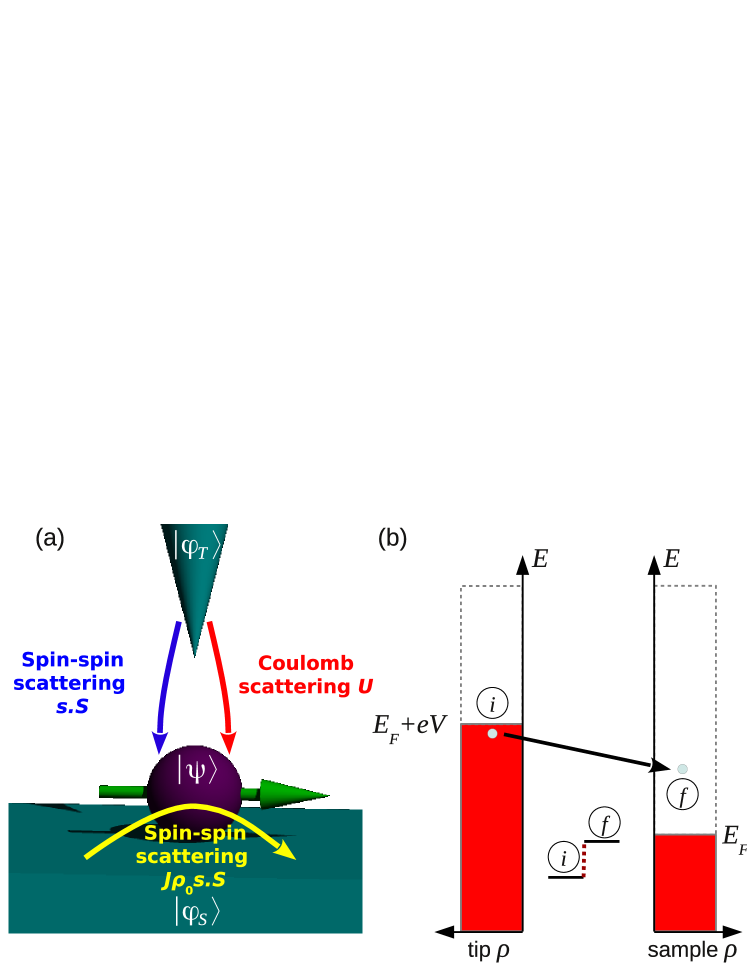
Figure 3: Model of the tunneling process between tip and sample. (a) Electrons originating from the tip interact with the localized spin system either via spin-spin (blue arrow) or potential scattering (red arrow). Additionally, we allow for spin-spin exchange scattering between sample electrons and the localized spin (yellow arrow). (b) Scheme of the first order Born approximation: In the tunneling process of an electron from the initial state $i$ to the final state $f$ it exchanges angular momentum and energy with the localized spin system. (c) In second order Born approximation the system additionally occupies an intermediate state $m$. This process produces characteristic logarithmic features in the tunneling spectrum.

2.1 Current and conductance in second order

We will now briefly review the calculation of the tunneling current using Fermi’s golden rule. In STM experiments the bias $eV$ applied between tip and sample shifts the Fermi level $\epsilon_{F}$ of the tip with respect to the one of the sample. At positive electrons from occupied tip states can cross the tunnel-barrier and interact with the localized spin system under exchange of angular momentum and energy (Figure 3b). To obey energy conservation, the energy difference $\epsilon_{if}=\epsilon_{f}-\epsilon_{i}$ between initial and final state of the spin system has to be accounted for by the energy of the tunneling electron. The current flowing between tip and sample is then given by:

$$I^{\rm t\rightarrow s}(eV)=\frac{2\pi e}{\hbar}T_{0}^{2}\sum_{i,f}p_{i}\int\limits_{-\infty}^{+\infty}\left|\mathcal{M}_{if}^{\rm t\rightarrow s}\right|^{2}f(\epsilon-eV)\left[1-f(\epsilon-\epsilon_{if})\right]d\epsilon,$$

$$I^{\rm s\rightarrow t}(eV)=\frac{2\pi e}{\hbar}T_{0}^{2}\sum_{i,f}p_{i}\int\limits_{-\infty}^{+\infty}\left|\mathcal{M}_{if}^{\rm s\rightarrow t}\right|^{2}f(\epsilon+eV)\left[1-f(\epsilon-\epsilon_{if})\right]d\epsilon,$$

$$I=I^{\rm t\rightarrow s}-I^{\rm s\rightarrow t},$$ (9)

where we have dropped the additional summation that would account for current through the different sites in coupled spin systems, i. e. we restrict our calculation to single spin systems.

The unitless tunnel barrier transmission coefficient $T_{0}^{2}=|T_{ta}J\rho_{s}|^{2}$ contains all experimental parameters that will determine the strength of the tunneling current. In particular, $T_{0}$ strongly depends on the distance between tip and adsorbate, and on the spin independent local densities of states in tip and sample. For the moment we want to assume that $T_{0}^{2}\ll 1$ so that the influence of the tip on the spin system is negligible and the time between consecutive tunneling events is much longer than the relaxation time of the spin system, e. g. via processes such as described by equation 8. Such conditions are usually easy to provide in STM experiments where the tip-sample separation can be adjusted to give tunneling currents in the pA range or below so that the tip can be seen as a local probe of the spin system that leaves the spins always in thermal equilibrium with the substrate (zero-current approximation).

Under this assumption the average state occupation $p_{i}(T)$ of the spin system is only governed by the effective temperature $T$ and follows the Boltzmann distribution,

$$p_{i}(T)=\frac{\exp[-\epsilon_{i}/(k_{B}T)]}{\sum_{i}\exp[-\epsilon_{i}/(k_{B}T)]},$$ (10)

with $k_{B}$ as the Boltzmann constant. Furthermore, we assume a flat density of states in tip and sample so that the electron occupation is given by the Fermi-Dirac distribution $f(\epsilon)=[1+\exp(\epsilon/k_{B}T)]^{-1}$.

While most STM experiments do not record the tunneling current directly, we are interested in its derivative with respect to the bias voltage. With the energy independent matrix elements the derivative of the current is easy to evaluate. Integrating the Fermi-Dirac distributions of equation 2.1 and calculating the derivative results in a temperature broadened step function [98]:

$$\Theta(x)=\frac{1+(x-1)\exp(x)}{\exp(x)^{2}},$$ (11)

with $x=\epsilon/(k_{B}T)$, so that equation 2.1 becomes:

$$\frac{{\partial}I}{\partial V}(eV)^{\rm t\rightarrow s}=\frac{2\pi e^{2}}{\hbar}T_{0}^{2}\sum_{i,f}p_{i}\left|\mathcal{M}_{if}^{\rm t\rightarrow s}\right|^{2}\Theta(eV-\epsilon_{if}).$$ (12)

The main goal of this paper lies in deriving the transition matrix elements $\mathcal{M}_{if}$ to be able to solve the equation 12. First, we start with second order processes, neglecting scattering that involves electrons which originate and end in the substrate bath, i. e. we concentrate on tunneling processes which consist of only one scattering event as depicted in figure 3b and described by the transport Hamiltonian of equations 6 and 7:

$$\mathcal{M}^{(1)}_{if}=\left\langle\varphi_{f},\psi_{f}\right|\frac{1}{2}\hat{\bm{\sigma}}\cdot\hat{\bf S}+U\hat{I}\left|\varphi_{i},\psi_{i}\right\rangle=M_{if}+U\delta_{if}.$$ (13)

This matrix is energy independent and connects the initial states in the electron baths $\left|\varphi_{i}\right\rangle$ and spin system $\left|\psi_{i}\right\rangle$ with their final states $\left|\varphi_{f}\right\rangle$ and $\left|\psi_{f}\right\rangle$. It contains the spin-exchange scattering term $M_{if}$ and a potential scattering term that has non-zero matrix-elements only when initial and final spin state are the same ($\delta_{if}$ is the delta distribution). Computing the absolute square of $\mathcal{M}^{(1)}_{if}$ results in three terms that contribute to the tunneling conductance:

$$\left|\mathcal{M}^{(1)}_{if}\right|^{2}=\left|M_{if}\right|^{2}+|U|^{2}\delta_{if}+2\Re\left(U\times M_{if}\right)\delta_{if},$$ (14)

where $\Re(A)$ denotes the real part of the matrix $A$. The first term consist of the operators

$$\hat{\bm{\sigma}}\cdot\hat{\bf S}=\hat{\sigma}_{x}\hat{S}_{x}+\hat{\sigma}_{y}\hat{S}_{y}+\hat{\sigma}_{z}\hat{S}_{z}=\frac{1}{2}\hat{\sigma}_{+}\hat{S}_{-}+\frac{1}{2}\hat{\sigma}_{-}\hat{S}_{+}+\hat{\sigma}_{z}\hat{S}_{z},$$ (15)

which connect the initial and final state and accounts for spin-exchange processes in which angular momentum between the tunneling electron and the localized spin system can be exchanged. The second term accounts for potential scattering between the tunneling electron and the localized spin system and does not change the spin state. The third term results from the interference between potential and spin-exchange scattering and depends, as we will see, strongly on the angular momentum of the localized spin and is the origin of magneto-resistive tunneling [13, 99].

Due to the product-state of the total quantum-mechanical system, it is worth mentioning that the matrix elements have to be independently evaluated for the localized spin and for the tunneling electron. For an electron tunneling between a spin-average tip and sample the non-zero matrix elements are:

$$\mbox{(a) }\langle\uparrow|\hat{s}_{+}|\downarrow\rangle=+1,\quad\mbox{(c) }\langle\uparrow|\hat{s}_{z}|\uparrow\rangle=+1/2,\quad\mbox{(e) }\langle\uparrow|\hat{I}|\uparrow\rangle=+1,$$

$$\mbox{(b) }\langle\downarrow|\hat{s}_{-}|\uparrow\rangle=+1,\quad\mbox{(d) }\langle\downarrow|\hat{s}_{z}|\downarrow\rangle=-1/2,\quad\mbox{(f) }\langle\downarrow|\hat{I}|\downarrow\rangle=+1,$$ (16)

where, for completeness, we have additionally included the probability amplitudes for interacting with the unity operator $\hat{I}$. Since $\hat{\sigma}=2\hat{s}$, these matrix elements enable us to rewrite the spin-exchange scattering term in equation 14 for a spin-average tip and sample to [8, 99]:

$$|M_{if}|^{2}=\frac{1}{2}\left|\left\langle\psi_{f}\right|\hat{S}_{-}\left|\psi_{i}\right\rangle\right|^{2}+\frac{1}{2}\left|\left\langle\psi_{f}\right|\hat{S}_{+}\left|\psi_{i}\right\rangle\right|^{2}+\left|\left\langle\psi_{f}\right|\hat{S}_{z}\left|\psi_{i}\right\rangle\right|^{2}.$$ (17)

Note, that 16c and 16d do not cancel out because the two different spin directions in the initial (tip or sample) and final (sample or tip) bath are incoherent ensemble states and therefore cannot interfere with each other.

For a tip with spin polarization $\eta=\left|\frac{\rho_{\uparrow}-\rho_{\downarrow}}{\rho_{\uparrow}+\rho_{\downarrow}}\right|$ along the $z$-axis, the transition matrix elements are tunnel-direction dependent because either the initial or the final electron bath has now a spin imbalance in the density of states [99]:

$$|M_{if}^{\rm t\rightarrow s}|^{2}=\frac{1+\eta}{2}\left|\left\langle\psi_{f}\right|\hat{S}_{-}\left|\psi_{i}\right\rangle\right|^{2}\!+\frac{1-\eta}{2}\left|\left\langle\psi_{f}\right|\hat{S}_{+}\left|\psi_{i}\right\rangle\right|^{2}\!+\left|\left\langle\psi_{f}\right|\hat{S}_{z}\left|\psi_{i}\right\rangle\right|^{2}$$

$$|M_{if}^{\rm s\rightarrow t}|^{2}=\frac{1-\eta}{2}\left|\left\langle\psi_{f}\right|\hat{S}_{-}\left|\psi_{i}\right\rangle\right|^{2}\!+\frac{1+\eta}{2}\left|\left\langle\psi_{f}\right|\hat{S}_{+}\left|\psi_{i}\right\rangle\right|^{2}\!+\left|\left\langle\psi_{f}\right|\hat{S}_{z}\left|\psi_{i}\right\rangle\right|^{2}.$$ (18)

As an example figure 4 shows the spectrum for a single spin with $S=1/2$. When applying the magnetic field, the conductance increases step-like at bias energies above the Zeeman-energy $|eV|>g\mu_{B}|B|$. These steps are symmetrical around zero voltage and thermally smeared out by about $5k_{B}T$ [98]. When the electrons in the tip are spin-polarized the step heights at positive and negative bias are different. For a paramagnetic tip with a spin polarization in direction of the applied field ($\eta>0$) the conductance step at positive bias decreases, while it increases by the same amount at negative bias (Figure 4b).

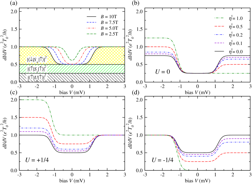
Figure 4: Tunneling spectra for a $S=1/2$ system at a temperature of $T=1$ K and $g=2$ evaluated in second order perturbation theory. (a) At applied magnetic field temperature broadened symmetric steps are visible. The different contributions to the conductance are labeled. Gray: conductance due to potential scattering ($|U|=0.25$), green: due to spin-spin scattering without changing the localized spin, yellow: spin-spin scattering with changing the spin. (b)–(d) A spin polarized tip produces asymmetric steps. Here, the zero voltage conductance depends strongly on the potential scattering $U$ and the tip polarization.

With a spin-polarized tip the interference between the potential and Kondo-scattering shows a very particular effect [13, 99]. Depending on the sign of $U$ the zero-bias conductance is either increased or reduced and can become even zero at $\eta=1$ and $U=-\frac{1}{2}S$ (Figure 4c-d). This magneto-resistive elastic tunneling [99] arises from the third term in equation 14 and scales with the expectation value $\langle\hat{S}_{z}\rangle$ of the impurity. At non-equilibrium the strength and sign of this term can change; this allows to read-out of the $z$-projection of the spin without exciting it, as has been shown in spin-pumping (see section 5) [13, 99] and pump-probe experiments [14].

2.2 Expansion to third order

We now turn our attention to the next higher order of interaction. We want to consider processes in which, during the transport of an electron from tip to sample (or vice versa), the spin system additionally interacts with an electron from the sample bath (Figure 3c). These processes involve an intermediate state ($m$) and are expressed in second order Born approximation as:

$$\mathcal{M}^{(2)}_{if}=J\rho_{s}\sum\!\!\!\!\!\!\!\!\int_{m}\left(\frac{\tilde{M}_{mf}M_{im}}{\epsilon_{i}-\epsilon_{m}}+\frac{M_{mf}\tilde{M}_{im}}{\epsilon_{m}-\epsilon_{f}}\right).$$ (19)

Here, the tilde on the matrix $\tilde{M}$ tags scattering processes between the localized spin and sample electrons only. The order of the two different electron-spin interactions can be exchanged. Thus, we have also to account for processes in which first an electron that originates and ends in the sample scatters the system into the intermediate state and then the tunneling electron interacts with the system scattering it into its final state (right fraction in equation 19). Here, it is of fundamental importance to have in mind that, contrary to the initial and final state of the total system, the intermediate state $|\psi_{m}\rangle$ can be virtual, i. e., must not necessarily obey angular momentum and energy conservation. The integro-summation symbol in equation 19 indicates that we perform both, a summation over all possible discrete intermediate states in the local spin system $|\psi\rangle$ and an integration over the continuous states of the intermediate electron states $|\varphi\rangle$ in the substrate. For the integration, we consider states in an energy range of $\pm\omega_{0}$ around $E_{F}$ as possible scatterer leading to the following characteristic function for electron-like processes [97, 100]:

$$F_{e}(\epsilon,T)=-\int\limits_{-\infty}^{+\infty}d\epsilon^{\prime\prime}\int\limits_{-\omega_{0}}^{+\omega_{0}}d\epsilon^{\prime}\frac{1-f(\epsilon^{\prime},T)}{\epsilon^{\prime}-\epsilon^{\prime\prime}}f^{\prime}(\epsilon^{\prime\prime}-\epsilon,T),$$ (20)

and for hole-like processes:

$$F_{h}(\epsilon,T)=-\int\limits_{-\infty}^{+\infty}d\epsilon^{\prime\prime}\int\limits_{-\omega_{0}}^{+\omega_{0}}d\epsilon^{\prime}\frac{f(\epsilon^{\prime},T)}{\epsilon^{\prime}-\epsilon^{\prime\prime}}f^{\prime}(\epsilon^{\prime\prime}-\epsilon,T),$$ (21)

respectively. Here, the Fermi-Dirac distributions in the numerator ensure an unoccupied (occupied) final state and the integration over the derivative $f^{\prime}$ accounts for the temperature broadening during the total process (Figure 5a). The switching from virtual to real processes at $\epsilon=0$ leads to a logarithmic singularity that is broadened by the temperature. Thus, as long as the energy $\epsilon_{m}$ of the intermediate state and the temperature $k_{B}T$ are small compared to the integration bandwidth $\omega_{0}$, the equations 20 and 21 (with a change of sign) can be rewritten as:

$$F(eV-\epsilon_{m})\approx-\int\limits_{-\infty}^{+\infty}d\epsilon^{\prime}\ln\left(\frac{\omega_{0}+|eV-\epsilon_{m}|}{eV-\epsilon_{m}+i\Gamma_{0}}\right)\times\Theta^{\prime}(eV-\epsilon_{m}+\epsilon^{\prime},T).$$ (22)

Here, $\Theta^{\prime}(\epsilon,T)=\partial\Theta(\epsilon,T)/\partial\epsilon$ is the derivative of the temperature broadened step function (equation 11) and a small $\Gamma_{0}$ accounts for additional non-thermal (lifetime) broadening. Figure 5 shows the energy and temperature dependence of $F$ which has first been experimentally observed on a radical molecule adsorbed on a Au(111) surface (see figure 1e and f) [22]. Compared to the Lorentzian or Frota functions [101] normally used for describing Kondo resonances in STM measurements [12], the behavior of this function is quite different, even though – if analyzed only in a small energy range of a few $k_{B}T$ around zero –, it has a similar shape [22]. The function shows a relatively flat top whose width is determined only by the temperature. For energies $k_{B}T<|\epsilon|<\omega_{0}$ the amplitude decays logarithmically as $-\ln(|\epsilon/\omega_{0}|)$ while the maximum peak height is proportional to $-\ln(k_{B}T/\omega_{0})$. Due to the restriction to states in an energy interval $\pm\omega_{0}$ the function remains analytical even at $\epsilon\rightarrow\pm\infty$ where $F$ approaches zero. Note, that the precise value of the cut-off energy $\omega_{0}$ is not critical and mainly changes only the background offset. If not otherwise noted we use $\omega_{0}=20$ meV throughout the paper.

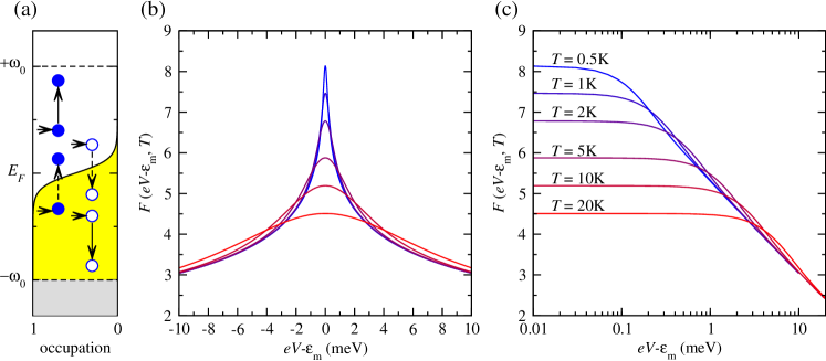
Figure 5: (a) Scheme of the third order processes. Full (dashed) vertical arrows illustrate real (virtual) transitions between intermediate and final state ($m\rightarrow f$) of electron-like (full circles) and hole-like (empty circles) carriers. (b) and (c) The temperature broadened logarithmic function $F(eV-\epsilon_{m},T)$ at different temperatures $T$ with $\omega_{0}=200$ meV and $\Gamma_{0}=5$ $\mu$eV. (b) linear, (c) linear-log plot.

When calculating the conductance we now have to consider both processes depicted in Figure 3b and c and thus have to replace $\mathcal{M}_{1}$ with $\mathcal{M}_{1}+\mathcal{M}_{2}$ in equation 12 leading to:

$$\left|\mathcal{M}^{(1)}_{if}+\mathcal{M}^{(2)}_{if}\right|^{2}= \left|\mathcal{M}^{(1)}_{if}\right|^{2}+$$

$$J\rho_{s}\sum_{m} \left[\left(M_{fi}\tilde{M}_{mf}M_{im}+\overline{M_{fi}\tilde{M}_{mf}M_{im}}\right)F(\epsilon_{mi})+\right.$$

$$\left.\left(M_{fi}M_{mf}\tilde{M}_{im}+\overline{M_{fi}M_{mf}\tilde{M}_{im}}\right)F(\epsilon_{im})\right]\!+$$

$$J\rho_{s}U\sum_{m} \left[\left(I_{fi}\tilde{M}_{mf}M_{im}+\overline{I_{fi}\tilde{M}_{mf}M_{im}}\right)F(\epsilon_{mi})+\right.$$

$$\left.\left(I_{fi}M_{mf}\tilde{M}_{im}+\overline{I_{fi}M_{mf}\tilde{M}_{im}}\right)F(\epsilon_{im})\right]\!+$$

$$\Or\left(J\rho_{s}\right)^{2}.\!\!\!\!$$

The evaluation of the matrix elements up to third order yields two new terms due to the interference between the processes described by $\mathcal{M}_{1}$ and $\mathcal{M}_{2}$ which are absent in the second order perturbation calculation. The term 23 was first identified by Jun Kondo [34] and can lead to temperature broadened logarithmic features in the conductance at the energy of intermediate states. For a non-vanishing potential scattering amplitude $(U\neq 0)$ the term 23 will, in addition, produce a bias-asymmetry in the differential conductance even without spin-polarized electrodes.

We start with the evaluation of the Kondo-like processes, that are described by the term 23, using a spin $S=1/2$ system with only two states as an example. We assume that in thermal equilibrium only the ground state $\left|\uparrow\right\rangle=\left|\psi_{1}\right\rangle$ is occupied, i. e. that the Zeeman-splitting induced by the external magnetic field is large compared to the thermal energy: $g\mu_{B}|B|\gg k_{B}T$. The Feynman diagrams of figure 6 depict all possible interaction processes.

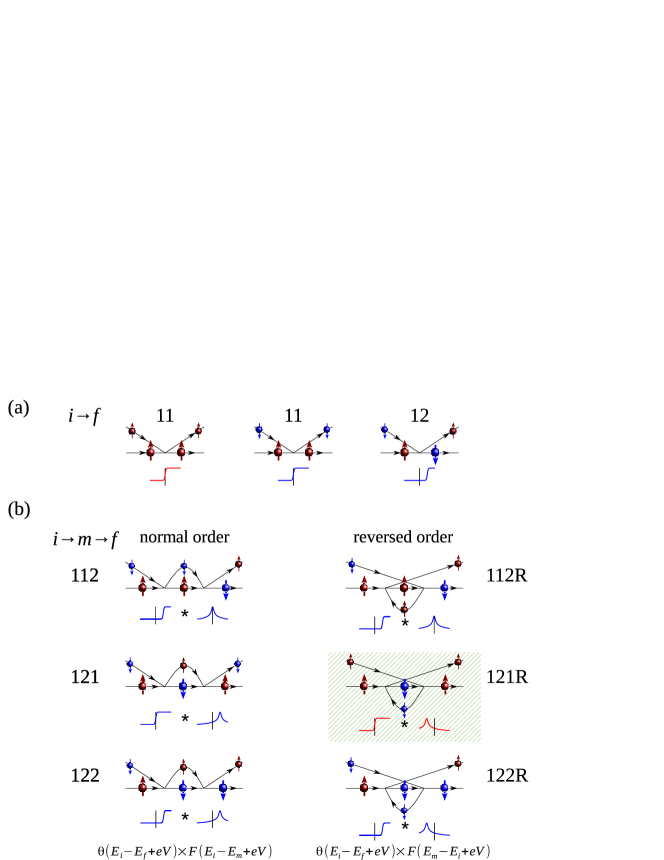
Figure 6: Interaction diagrams of order two (a) and three (b) for an electron tunneling from tip to sample into a two level $S=1/2$ spin system. The large (small) spheres depict the state of localized spin (interaction electron) and the color their spin directions. Schematic spectra show their contributions to the conductance at positive bias. The numbers label the processes with the state order of the localized spin-system. An appended ’R’ label processes in which the scattering into the intermediate state is performed before the tunneling electron interacts (exchange diagrams). Note that the time order of the processes influences crucially the conductance spectra as schematically displayed in the small graphs (vertical line is $E_{F}$; the $\ast$ means multiplication).

First, we review the second order processes (Figure 6a): A spin-up electron that tunnels from tip to the sample cannot flip the spin ($\left|\psi_{1}\right\rangle\rightarrow\left|\psi_{1}\right\rangle$), while a spin-down electron can either scatter with exchange of angular momentum ($\left|\psi_{1}\right\rangle\rightarrow\left|\psi_{2}\right\rangle$) leaving the system in the state $\left|\downarrow\right\rangle=\left|\psi_{2}\right\rangle$ or without exchange ($\left|\psi_{1}\right\rangle\rightarrow\left|\psi_{1}\right\rangle$). To third order, there are a total of six diagrams to be accounted for, which we can label by the states occupied in the initial ($i$), intermediate ($m$), and final ($f$) state. Here, we mark the exchange diagrams by appending a ’R’. This results in the processes (112), (121), (122), and the reversed order scattering events (112R), (121R), (122R).

To evaluate the conductance due to these processes we calculate the spin-flip matrix elements of equation 15 for the electrons and the localized spin-system. For electrodes without spin-polarization this results in conductances of:

$$\frac{\partial I}{\partial V}(eV)^{\rm t\rightarrow s}=\frac{4\pi e^{2}}{\hbar}T_{0}^{2}\frac{J\rho_{s}}{4i}\sum_{\genfrac{}{}{0.0pt}{}{j,k,l=}{\{x,y,z\}}}\varepsilon_{jkl}\Re\left[\left\langle\psi_{i}\right|\hat{S}_{l}\left|\psi_{f}\right\rangle\left\langle\psi_{f}\right|\hat{S}_{k}\left|\psi_{m}\right\rangle\left\langle\psi_{m}\right|\hat{S}_{j}\left|\psi_{i}\right\rangle\right]$$

$$\times F(eV-\epsilon_{im},T)\times\Theta(eV-\epsilon_{if},T),$$ (24)

$$\frac{\partial I}{\partial V}(eV)^{\rm t\stackrel{{\scriptstyle R}}{{\rightarrow}}s}=\frac{4\pi e^{2}}{\hbar}T_{0}^{2}\frac{J\rho_{s}}{4i}\sum_{\genfrac{}{}{0.0pt}{}{j,k,l=}{\{x,y,z\}}}\varepsilon_{jkl}\Re\left[\left\langle\psi_{i}\right|\hat{S}_{l}\left|\psi_{f}\right\rangle\left\langle\psi_{f}\right|\hat{S}_{k}\left|\psi_{m}\right\rangle\left\langle\psi_{m}\right|\hat{S}_{j}\left|\psi_{i}\right\rangle\right]$$

$$\times F(eV-\epsilon_{mi},T)\times\Theta(eV-\epsilon_{if},T).$$ (25)

Here, equation 24 accounts for the direct diagrams (normal order) and 25 for the exchange diagrams (reversed order), respectively. In these equations $\varepsilon_{jkl}$ is the usual Levi-Civita tensor of rank three, which is 1 (-1) if $\{jkl\}$ is an even (odd) permutation of $\{xyz\}$, and zero otherwise [77]. The step-function $\Theta$ ensures that energy conservation at the final state of the scattering process is obeyed, while the function $F$ has its peak at the intermediate state energy and is mirrored at $E_{F}$ for the reversed tunneling process. Any spin-polarization in tip or sample changes the transition matrix elements for the interacting electrons and equations 24 and 25 would become more complex (see A).

Comparing the different contributions to the conductance (figure 6b and 7a) it is remarkable that all third order scattering events start with a spin-down electron except the process $121R$. Here, a spin-up electron tunneling from tip to sample non-trivially interacts with the system because a substrate electron has flipped the localized spin into the intermediate spin-down state before the interaction takes place.

Summing up the contributions to the conductance due to all second and third order scattering events results in spectra similar to those exemplary given in figure 7b (c. f. figure 1e and f [22]).

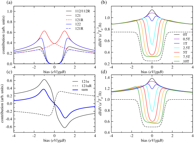
Figure 7: Tunneling spectra for a $S=1/2$ system (a) The third order contributions for non spin-polarized tip and sample with $k_{B}T=0.1\times g\mu_{B}B$ and $\omega_{0}=20\times g\mu_{B}B$. (b) Total conductance for $J\rho_{s}=-0.05$, $U=0$, $T=1$ K, and $g=2$ at different magnetic fields. (c) Additional contributions to the conductance in third order due to a non-zero potential scattering term. (d) Total conductance as in (b) but with $U=0.25$. Dashed lines in (b) and (d) show the second order conductance only at $B=10$ T.

At zero field the differential conductance shows a peak that splits with increasing magnetic field. While in this calculation we assume to be in the weak-coupling Kondo limit and thus neglect any correlation energy due to the formation of a Kondo singlet, the peak splits as soon as the Zeeman energy overcomes the thermal energy. Note, that the resulting split-peak at small fields can lead to the deduction of an erroneously high $g$-factor when just evaluating the peak positions due to the superposition of peak and step-structures.

If we consider now in addition that the scattering process between tip and sample or vice versa can also occur via the potential interaction (term 23), we observe an asymmetric line-shape as soon as the two eigenstates are no longer degenerate and $\langle\hat{S_{z}}\rangle\neq 0$ (figure 7c and d). This direction-dependent asymmetry cannot originate from the scattering matrix elements that involve only the localized spin site (the order of excitations shall be the same) but derives from the matrix elements involving the interacting electrons. Physically, the reason lies in the asymmetry of the tunnel-junction for which we assume that only the sample is coupled to the spin-system and thus neglect any intermediate scattering process that originate and end in the tip.

As an example, we examine in detail the process (121) (see figure 6b) in both tunneling directions. For a current to flow from tip to sample via this process, first a $\left|\downarrow\right\rangle$ electron originating from the tip is scattered into a $\left|\uparrow\right\rangle$ state in the sample exciting the spin system from $\left|\psi_{1}\right\rangle\rightarrow\left|\psi_{2}\right\rangle$. Second, a $\left|\uparrow\right\rangle$ electron in the sample is scattered into $\left|\downarrow\right\rangle$ bringing the spin system back to $\left|\psi_{1}\right\rangle$. Third, the sample $\left|\downarrow\right\rangle$ is scattered back into the tip as $\left|\downarrow\right\rangle$ electron. The last step of this process can either take place via the $\hat{\sigma}_{z}$ or, in the case of potential scattering, via the $\hat{\sigma}_{I}$ term, respectively. For an electron tunneling in the reverse direction we first have a $\left|\downarrow\right\rangle$ from the sample being scattered into an electron $\left|\uparrow\right\rangle$ state of the tip simultaneously exciting the spin system from $\left|\psi_{1}\right\rangle\rightarrow\left|\psi_{2}\right\rangle$. Then, the second process flips a $\left|\uparrow\right\rangle$ sample electron into the $\left|\downarrow\right\rangle$ hole from the first process. Finally, a $\left|\uparrow\right\rangle$ tip electron traverses the junction and fills the $\left|\uparrow\right\rangle$ hole in the sample. Comparing both tunneling directions we see that it is the third process which differs in the initial and final state, i. e. the matrix elements are either $\langle\downarrow|\hat{\sigma}_{z}|\downarrow\rangle$ and $\langle\downarrow|\hat{\sigma}_{I}|\downarrow\rangle$ or $\langle\uparrow|\hat{\sigma}_{z}|\uparrow\rangle$ and $\langle\uparrow|\hat{\sigma}_{I}|\uparrow\rangle$. Rearranging the matrix elements so that all processes become electron-like, the prefactors for calculating the tunneling conductance due to these four processes are for the two without potential scattering:

$$(121)^{{\rm t}\rightarrow{\rm s}}:\quad +J\rho_{s}\underbrace{\langle\downarrow^{\rm t}|\hat{\sigma}_{z}|\downarrow^{\rm s}\rangle}_{-}\underbrace{\langle\downarrow^{\rm s}|\hat{\sigma}_{-}|\uparrow^{\rm s}\rangle}_{+}\underbrace{\langle\uparrow^{\rm s}|\hat{\sigma}_{+}|\downarrow^{\rm t}\rangle}_{+} >0$$

$$(121)^{{\rm s}\rightarrow{\rm t}}:\quad -J\rho_{s}\underbrace{\langle\uparrow^{\rm t}|\hat{\sigma}_{+}|\downarrow^{\rm s}\rangle}_{+}\underbrace{\langle\downarrow^{\rm s}|\hat{\sigma}_{-}|\uparrow^{\rm s}\rangle}_{+}\underbrace{\langle\uparrow^{\rm s}|\hat{\sigma}_{z}|\uparrow^{\rm t}\rangle}_{+} >0,$$ (26)

and with potential scattering:

$$(121u)^{{\rm t}\rightarrow{\rm s}}:\quad +J\rho_{s}U\underbrace{\langle\downarrow^{\rm t}|\hat{\sigma}_{I}|\downarrow^{\rm s}\rangle}_{+}\underbrace{\langle\downarrow^{\rm s}|\hat{\sigma}_{-}|\uparrow^{\rm s}\rangle}_{+}\underbrace{\langle\uparrow^{\rm s}|\hat{\sigma}_{+}|\downarrow^{\rm t}\rangle}_{+} <0$$

$$(121u)^{{\rm s}\rightarrow{\rm t}}:\quad -J\rho_{s}U\underbrace{\langle\uparrow^{\rm t}|\hat{\sigma}_{+}|\downarrow^{\rm s}\rangle}_{+}\underbrace{\langle\downarrow^{\rm s}|\hat{\sigma}_{-}|\uparrow^{\rm s}\rangle}_{+}\underbrace{\langle\uparrow^{\rm s}|\hat{\sigma}_{I}|\uparrow^{\rm t}\rangle}_{+} >0,$$ (27)

where we assumed $J\rho_{s}<0$ and $U>0$. Note, that the preceding sign change at the tunneling direction from sample to tip (${\rm s}\rightarrow{\rm t}$) is due to the rearrangement of the interaction order together with the switching from hole-like to electron-like scattering. The contribution to the conductance from the processes in which only Kondo-like spin-spin interactions take place is positive for both tunneling directions, while the conductance for processes that include potential scattering changes its sign when inverting the tunneling direction.

3 Some single spin examples

Up to here we have revised the relevant formalism to calculate the conductance in the third order of the matrix elements quite closely following the work established by Appelbaum, Anderson, and Kondo [34, 95, 96, 97]. The $S=1/2$ system we used for illustration contained only two states and was not influenced by any magnetic anisotropy or near-by spin systems. Recently, efforts have been made to expand this perturbative model to higher spin systems, which also include magnetic anisotropy and couplings to neighboring spins [84, 85, 83, 81], but the importance of the potential scattering was not taken into account up to now. In the following, the power of this easily accessible model will be used to evaluate and describe the spectral features on more complex systems.

3.1 The smallest ($S=$1) high-spin system

Regarding the spectra of the $S=1/2$ system (Figure 7), one could get the impression that the coupling to the sample always results in some superimposed peak-like structures as soon as a spin flip transition is possible, and which scales with the substrate coupling strength $-J\rho_{s}$. In this section we will show that the situation is more complex and depend not only on the transition matrix elements but also on the state energies.

To expand the complexity, we turn now to a magnetic system with $S=1$ in which axial and transverse magnetic anisotropy have broken the zero-field degeneracy of the three eigenstates. Assuming easy-axis anisotropy ($D<0$) the energetically lowest eigenstates have weights only for $m_{z}=\pm 1$. The additional transverse anisotropy splits the remaining two-fold degeneracy forming an antisymmetric ground and a symmetric first excited state (Figure 8a). Thus, in the basis of the magnetic easy axis the three eigenstates can be written as: $\left|\psi_{1}\right\rangle=\frac{1}{\sqrt{2}}(\left|+1\right\rangle-\left|-1\right\rangle)$, $\left|\psi_{2}\right\rangle=\frac{1}{\sqrt{2}}(\left|+1\right\rangle+\left|-1\right\rangle)$, and $\left|\psi_{3}\right\rangle=\left|0\right\rangle$. Such situations have been found for example for Fe(II)-phthalocyanine molecules adsorbed on the ($2\times 1$) oxygen terminated Cu(110) surface [65], for Fe atoms adsorbed on InSb(110) [53], or for CoH complexes adsorbed on the $h$-BN/Rh(111) surface [51].

By taking only second order spin-flip processes into account it is easy to calculate (using equation 17) that the transition probabilities from the groundstate to the two excited states at $B=0$ are equal, leading to a symmetric double step structure in the spectrum (Figure 8). Expanding the calculation to third order, only the processes which involve all states, i. e. (123) and (132), have non-zero matrix elements when the potential scattering $U=0$. Processes like (112), (121), or (131) cannot be interlinked using any combination of the operators $\hat{S}_{+}$, $\hat{S}_{-}$, and $\hat{S}_{z}$ and are thus forbidden. Nevertheless, additional potential scattering enables transitions involving the operators $\hat{S}_{+}$, $\hat{S}_{-}$, and $\hat{I}$ or $\hat{S}_{z}$, $\hat{S}_{z}$, and $\hat{I}$ which makes the aforementioned processes possible resulting in an asymmetry of the spectrum with respect to tunneling direction.

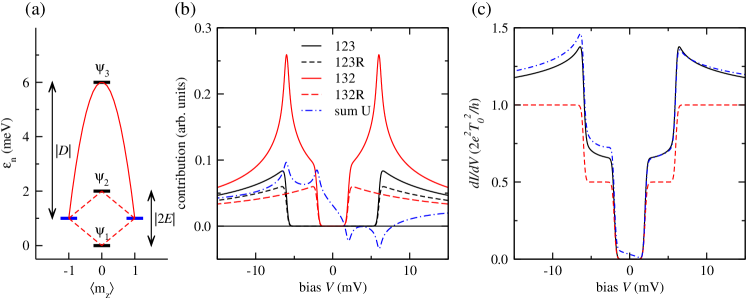
Figure 8: Tunneling spectra of a spin $S=1$ system. (a) The anisotropy lifts all degeneracies ($D=-5$ meV, $E=1$ meV) at zero field. The plot shows the state energy over the $m_{z}$ expectation value $\langle m_{z}\rangle=\tr\left(\hat{S}_{z}\left|\psi_{i}\right\rangle\left\langle\psi_{i}\right|\right)$ (blue: $E=0$, black: $E\neq 0$) (b) The significant third order processes ($T=1$ K, $B=0$ T). The dot dashed line show the additional contribution for a $U=0.125$. (c) The total spectrum with $J\rho_{s}=0$ (dashed red line), $-0.1$ (full black line), and with additional $U=0.125$ (dotted dashed blue line).

It is remarkable that the remaining third order processes at $U=0$ change the spectrum in a quite different fashion, even though they have the same strength. Process (123) produces its peaks at $eV=\pm\epsilon_{2}$, but due to energy conservation it contributes to the spectrum only at $|eV|>\epsilon_{3}$, which efficiently cuts off the peak. In contrast, the peak at higher energy due to process (132) is not as strongly cut off (Figure 8b). Thus, the full spectrum shows a peak-like increase of the conductance at the energy of the second step but not at the energetically lower first transition step. Furthermore, the conductance has a curved form for tunneling voltages between $\epsilon_{2}$ and $\epsilon_{3}$ (Figure 8c). Note, the overall general behavior would not alter when changing from easy-axis to easy-plane anisotropy ($D>0$) as long as all degeneracies are lifted.

3.2 Single Mn and Fe atoms on Cu₂N

After the, with only three eigenstates, rather easy $S=1$ example, we now apply the model to the experimentally and theoretically intensively studied single 3d transition metal atoms adsorbed on a monolayer of Cu₂N on Cu(100). When these atoms are placed on top of a Cu site they form strong covalent bonds with the neighboring N atoms [8]. This highly anisotropic adsorption geometry leads to three distinct symmetry axes that are perpendicular to each other: The direction out-of-surface and two in-surface directions along the Cu-N bonds and perpendicular to it, along the so called vacancy rows (Figure 9a inset).

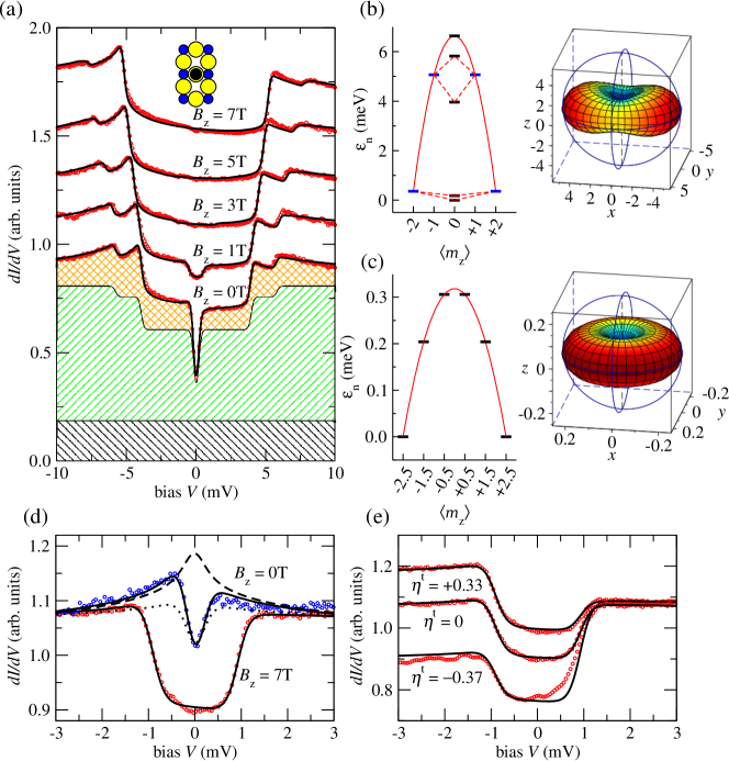
Figure 9: Comparison of experimental and calculated spectra on Fe and Mn atoms adsorbed on Cu₂N. (a) Experimental data from ref. [8] measured on a single Fe atom at increasing field $B_{z}$ along the easy axis and at a temperature $T=550$ mK (red circles). The simulations (black lines) for all plots are obtained with one set of parameters: $g=2.11$, $D=-1.57$ meV, $E=0.31$ meV, $J\rho_{s}=-0.087$, $U=0.35$, and $T_{\rm eff}=740$ mK. Additionally, a constant offset of $\approx 20$% of the total conductance had to been added (black shaded area). For $B_{z}=0$ the second (green shaded area) and third order (orange hatched area) contributions to the conductance are indicated. The spectra at field are vertically shifted for better visibility. The inset shows the adsorption site of the 3d atoms (black circle) on the Cu₂N (Cu yellow, N blue circle) (b) and (c) Schematic state diagrams and visualizations of the magnetic anisotropy (in meV) for Fe (b) and Mn (c) [89]. (d) Experimental data of two different Mn atoms at $B_{z}=0$ and $B_{z}=7$ T (colored circles). The fits (full lines) for the $B_{z}=0(7)$T data results in $J\rho_{s}=-0.029(-0.0091)$, $U=1.35(1.28)$, $D=-51(-39)\ \mu$eV, $g=1.9$, and $T_{\rm eff}=790(930)$ mK. The dashed line simulates for the zero field data the absence of any anisotropy. The dotted line simulates with the 7 T parameters the absence of a magnetic field. (e) The 7 T atom as in (d) probed with tips of different spin polarizations $\eta^{\rm t}$ (Data from ref. [99]).

Single Fe atoms adsorbed on this surface have been found to be in the $S=2$ state with a magnetic easy-axis along the N rows ($z$-direction) and a magnetically hard-axis along the vacancy row ($x$-direction). In this coordinate system anisotropy values of $D=-1.55$ mV and $E=0.31$ mV, and a gyromagnetic factor of $g=2.11$ described the experimental data well using a spin Hamiltonian like equation 5 and a second order tunneling model [8, 75, 102]. The Hamiltonian has as solution five non-degenerate eigenstates and, due to $D<0$, favors, at zero field, ground states with weights at high $m_{z}$ values. Similar to the $S=1$ system the transverse anisotropy breaks the degeneracies leading to a symmetric and antisymmetric solution with the main weights at $\left|\pm 2\right\rangle$ as ground and first excited state and weights in $\left|\pm 1\right\rangle$ for the second and third excited state (Figure 9b). To visualize the anisotropy we plot the total energy necessary to rotate the ground state into arbitrary directions showing the favored easy axis ($z$) and the unfavored hard axis ($x$) (Figure 9b) [89]. In second order, spin-flip scattering is allowed between the groundstate and the three lowest excited states but a transition to the highest state is forbidden because this would require an exchange of $\Delta m=\pm 2$.

Experimental $dI/dV$ measurements on this system show, in addition to the conductance steps, peak-like structures at the second and third step but not at the lowest one (Figure 9a). Additionally, they show an asymmetry between positive and negative bias. To rationalize these observations we can follow a similar argumentation as in the $S=1$ case: In third order, transitions like (121) are not possible without additional potential interaction and processes like (123) or (124) are strongly cut off due to the high energy difference between $\epsilon_{2}$ and $\epsilon_{3}$ or $\epsilon_{4}$. In contrast, the processes (132) and (142) scale with $J\rho_{s}$ leading to the peak features in the differential conductance. The additional asymmetry hints at a non-negligible potential scattering. As the computed curves in figure 9a reveal, our model almost perfectly fits the magnetic field data without any adaption of the parameters. We mention that similar good agreement between experimental data and computation can be reached in the other two magnetic field directions (not shown). The coupling strength in these simulations is $J\rho_{s}=-0.087$, close to the $-0.1$ found in a similar perturbative approach [84]. A potential scattering term of $U=0.35$ is necessary to reproduce the asymmetry. This value is significantly smaller than the $U\approx 0.75$ found in experiments where the magneto-resistive elastic tunneling was probed [99]. Part of this discrepancy can be understood by an additional conductance term that does not coherently interact with the spin-system and which would lead to an overestimation of $U$ in magneto-resistive measurements. Indeed we need a constant conductance offset of about $20$%, which is added to the calculated conductance to reproduce the spectra.

Switching from an integer to a half-integer spin system we now discuss individual Mn atoms on Cu₂N, which have a spin of $S=5/2$ and only a small easy-axis anisotropy of $D\approx-40\ \mu$eV along the out-of-plane direction and a negligible transverse anisotropy [7, 8]. The easy-axis anisotropy prohibits the immediate formation of a Kondo state due to a Kramer’s degenerate ground state doublet with $m_{z}=\pm 5/2$ (Figure 9c). At zero field a typical spectrum shows only one step, which belongs to the transition between the $\pm 5/2$ and the $\pm 3/2$ states that have superimposed asymmetric peak structures (Figure 9d). The fit to the model yields $J\rho_{s}=-0.029$ and resembles a $S=1/2$ split-Kondo peak at small magnetic fields (see figure 7b). A different Mn atom investigated at $B_{z}=7$ T shows a significantly reduced $J\rho_{s}=-0.0091$. Interestingly, we find for both atoms a potential scattering value of $U\approx\frac{1}{2}S$, which allows one to describe the spectra without the need of any additional conductance offset. This high $U$ value that is the origin of the bias asymmetry has been independently found in spin-pumping experiments [13] (see section 5) and by measuring the magneto-resistive elastic tunneling contribution [99]. The extraordinary agreement between model and experiment can be seen in measurements using different spin-polarized tips on the same atom (Figure 9e). Here, the strong influence of the tip-polarization on the inelastic conductance at bias voltages $|V|<1$ mV is evident while the differential conductance at $V>1.5$ mV stays, for all tips, constant.

4 The limit of the perturbative approach: The Kondo system Co on Cu₂N

When a half-integer spin with $S>1/2$ has easy-plane anisotropy $D>0$, its ground state at zero field is a doublet with its main weights in $m_{z}=\pm 1/2$. This enables an effective scattering with the substrate electrons and leads at low enough temperatures to the formation of a Kondo state. Experimentally this has been observed for Co atoms on Cu₂N [9, 11, 16, 17, 18] which have been found to have the total spin $S=3/2$ and which enter the correlated Kondo state with a characteristic Kondo temperature of $T_{K}=2.6$ K in experiments performed on small patches of Cu₂N at temperatures down to $T=550$ mK [9]. Apart from $D>0$ the system also has a small in-plane anisotropy ($E\neq 0$) which creates an easy axis ($x$) along the nitrogen row and a hard axis ($z$) along the vacancy rows (Figure 10a).

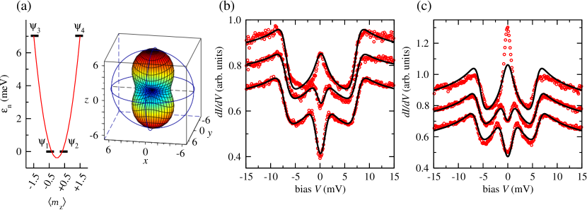
Figure 10: The tunneling spectra of Co atoms ($S=3/2$) on Cu₂N. (a) Schematic state diagram and visualizations of the magnetic anisotropy (in meV). At $B=0$ the states $|\psi\rangle_{1}$ and $|\psi\rangle_{2}$ are degenerated and differ by $\Delta m_{z}=\pm 1$. (b) and (c) Experimental data from reference [16] of two different Co atoms at $B_{x}=0,4,6$ T (colored circles, top to down, shifted for clarity). The best fits (full lines) results in $T_{\rm eff}=4$ K, $D=3.3$ meV, $E=0.7$ meV, $g=2$, $J\rho_{s}=-0.11$ for (b) and $T_{\rm eff}=3.8$ K, $D=2.7$ meV, $E=0.5$ meV, $g=2$, $J\rho_{s}=-0.25$ for (c), respectively.

Interestingly, in this system the coupling to the substrate $J\rho_{s}$ changes with the position of the Co atom on larger Cu₂N patches, concomitant with a change in the anisotropy energies which separates the $\left|\pm 1/2\right\rangle$ states from the $\left|\pm 3/2\right\rangle$ ones [16, 94]. For us this allows the study of the transition from the weak coupling to the strong coupling regime. In the case where the Co atom is relatively weakly coupled to the substrate ($J\rho_{s}\approx-0.1$), the model can be consistently fitted to the experimental data even at different field strengths along $B_{x}$ (Figure 10b). We observe a zero-energy peak that splits at applied fields similar to the $S=1/2$ system of figure 7d. But while for $S=1/2$ the field direction does not play a role, here the peak splitting depends strongly on the direction due to the magnetic anisotropy [9]. For this high-spin system we furthermore observe inelastic steps due to the transition to energetically higher excited states which are located at $|eV|=2|D|$ for $B=0$ and whose additional peak structure is well described within the model.

For Co atoms adsorbed closer to the edges of the Cu₂N patches, the coupling to the substrate increases and the fit to the model worsens significantly (Figure 10c). While the experimental data measured for non-zero fields are reasonable well described with $J\rho_{s}\approx-0.25$, at $B=0$ the experimentally detected peak at $E_{F}$ is stronger than the peak created by the model. Additionally, the experimental peak-width appears to be smaller than the temperature broadened logarithmic function, which was similarly observed for a radical molecule with $S=1/2$ for temperatures presumably close to $T_{K}$ [22]. Furthermore, we observe that the calculated spectrum no longer well describes the steps at $2|D|$. At this energy the third order contributions are less pronounced in the experimental data, indicating that we reach the limit of the perturbative approach.

The full description of a spin system in the strong coupling regime requires complex theoretical methods like numerical renormalization group theory [103, 36, 104] which are beyond the scope of this paper. Nevertheless, we can discuss some of the physical consequences within the outlined perturbative model. In contrast to the examples discussed in section 3, the two lowest degenerate ground states of the Co/Cu₂N system have weights in states that are separated by $\Delta m=\pm 1$. Thus, at zero field, electrons from the substrate can efficiently flip between these two states. The computation of the transition rate between the two states $|\psi_{i}\rangle$ and $|\psi_{f}\rangle$ of the spin system that have the energies $\epsilon_{i}$ and $\epsilon_{f}$ is $\Gamma_{if}:=I_{if}/e$, i. e. the transition probability per time, is analogous to the calculation of the current (equation 2.1) given by:

$$\Gamma_{if}^{\rm s\rightarrow s}=\frac{I_{if}^{\rm s\rightarrow s}}{e}=\frac{2\pi}{\hbar}(J\rho_{s})^{2}\int_{-\infty}^{\infty}d\epsilon\,|\mathcal{M}_{if}^{\rm s\rightarrow s}|^{2}f(\epsilon,T)[1-f(\epsilon-\epsilon_{if},T)].$$ (28)

Here we have set the bias to $eV=0$ and replaced the coupling constant $T_{0}$ between adsorbate and tip with $J\rho_{s}$, the coupling between adsorbate and substrate. When we now consider only processes up to second order, the matrix $\mathcal{M}_{if}$ is independent of the energy and the integral can be evaluated to

$$\int_{-\infty}^{\infty}d\epsilon\,f(\epsilon,T)[1-f(\epsilon-\epsilon_{if},T)]=\frac{\epsilon_{if}}{\exp\left(\frac{\epsilon_{if}}{k_{B}T}\right)-1}.$$ (29)

Thus, the scattering rate between the two degenerate states (i. e. $\epsilon_{12}=0$) is directly proportional to the temperature (Figure 11a):

$$\Gamma_{12}^{(2)\rm s\rightarrow s}=\frac{2\pi}{\hbar}(J\rho_{s})^{2}|\tilde{M}_{12}|^{2}k_{B}T.$$ (30)

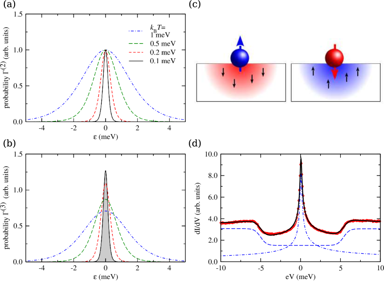
Figure 11: Correlations induced by substrate electrons. (a) In second order the scattering probability of a substrate electron with energy $\epsilon$ is given by the overlap of the electron and hole-like Fermi-Dirac distributions (area underneath the curve) and is for degenerated ground states directly proportional to the temperature. Third order scattering (b) gets logarithmically stronger than the second order processes with decreasing temperature. (c) Schematics of the entangled state at temperatures below the characteristic Kondo temperature. The scattering leads to a correlation between the spin state of the localized system and the sample electrons in the vicinity. (d) Spectrum of a Co adatom on Cu₂N in the Kondo regime ($B=0$ T, $T=0.55$ K, data from ref. [9]). The experimental $dI/dV$ curve (red dots) is well described by the sum (full line) of a Frota peak centered at $E_{F}$ (dotted dashed line) and a broadened step-function at higher energy (dashed line).

These scattering processes, which we have discussed in section 2 and displayed in figure 6a, will tend to change the spin polarization of the electronic states in the sample near the adsorbate to be correlated with the localized spin. Nevertheless, this local correlation will be quickly destroyed by decoherent scattering processes with the remaining electron bath, which we can assume to be large and dissipative. This decoherence rate is also proportional to the temperature, $\Gamma_{decoh}\propto k_{B}T$ [105], but usually stronger so that no highly correlated state can form. This picture changes when we additionally consider third order scattering processes which yield, using equation 23, the probability:

$$\Gamma_{if}^{(3)\rm s\rightarrow s}=\frac{4\pi}{\hbar}(J\rho_{s})^{3}\int_{-\infty}^{\infty}d\epsilon\,\sum_{m}\Re(\tilde{M}_{fi}\tilde{M}_{mf}\tilde{M}_{im})$$

$$\times\left[F(\epsilon_{mi}-\epsilon,T)+F(\epsilon_{im}-\epsilon,T)\right]f(\epsilon,T)[1-f(\epsilon-\epsilon_{if},T)].$$ (31)

Due to the growing intensity of $F(\epsilon=0)$ at reduced temperatures (Figure 5), for temperatures $T\rightarrow 0$ the scattering $\Gamma^{(3)}$ decreases significantly more slowly than $\Gamma^{(2)}$ (see figure 11b) so that their ratio steadily increases:

$$\frac{\Gamma^{(3)}}{\Gamma^{(2)}}\approx J\rho_{s}\ln\left(\frac{k_{B}T}{\omega_{0}}\right).$$ (32)

In contrast to that, the decoherent scattering rate with the bath $\Gamma_{decoh}$ lacks localized scattering centers and therefore has no significant third order contributions. Equation 32 leads to a characteristic temperature, the Kondo temperature $T_{K}$, where $\Gamma^{(3)}$ and higher order scattering terms become the dominant processes and perturbation theory breaks down [34, 106, 107, 36]:

$$T_{K}\approx\frac{\omega_{0}}{k_{B}}\exp\left(\frac{1}{J\rho_{s}}\right).$$ (33)

Below this temperature the assumption used up to now, i. e. that the electronic states in the sample are not influenced by the presence of the spin system, no longer applies. Using exact methods like the modified Bethe ansatz [108, 109] or numerical renormalization group theory [104] reveals that the sample electrons in the vicinity rather form an entangled state with the impurity, i. e.

$$\Psi^{total}=\frac{1}{\sqrt{2}}\left(\left|\downarrow^{\rm s}\right\rangle\left|+\frac{1}{2}\right\rangle-\left|\uparrow^{\rm s}\right\rangle\left|-\frac{1}{2}\right\rangle\right),$$ (34)

as illustrated in figure 11c. This combined state is quite complicated because the electronic states in the sample are continuous in energy and extend spatially, and therefore strongly alter the excitation spectrum of the adsorbate [110, 111].

Figure 11d shows the impact of the formation of the correlated state on the experimentally detected spectrum of the Co/Cu₂N system. At temperatures $T\ll T_{K}$, the peak at the Fermi energy can no longer be well reproduced by a temperature broadened logarithmic function (which in any case must diverge for $T\rightarrow 0$). The peak is much better described by an asymmetric Lorentzian, i. e. a Fano line-shape [47], or the Frota function [101, 112, 113] which has a finite amplitude and a half-width of $\Delta=k_{B}T_{K}$, corresponding to the correlation energy of the Kondo state. Superimposed on this zero-energy peak we detect conductance steps at voltages that enable scattering of the spin system into the $m_{z}=\pm 3/2$ state. These steps are well described using only a second order perturbation spin-flip model [9] and do not show any third order logarithmic contributions. This means that the probability of the third order scattering channels must be closed due to the ground-state correlation between the localized spin and the substrate electrons. Here we see that the simple perturbative approach of the model is no longer valid and fails to capture the full physics in this strongly coupled Kondo regime. Nevertheless, the model still gives valuable information because it enables us to identify the conditions under which correlations can evolve and is due to its computational simplicity also applicable for larger and more complex spin systems where the calculation of the exact solution might not be feasible or very time consuming.

5 Spin dynamics and rate equations

In the preceding section we discussed the appearance of correlations due to higher order scattering between the substrate electrons and the localized spin system. Now we want to evaluate how the tunneling of electrons between the biased tip and the sample influences the state populations and the observable spectroscopic features in local conductance measurements. This is equivalent to dropping the zero-current approximation we have assumed until now. We will see that the change of time-averaged system properties results in characteristic fingerprints in the $dI/dV$ signal which can become crucial for a deeper understanding of the system’s response and dynamics.

To describe the transition rate between the localized spin states $\left|\psi_{i}\right\rangle$ and $\left|\psi_{f}\right\rangle$ due to the tunneling current flowing between tip and sample we can again use equation 2.1 and the relation $\Gamma_{if}^{\rm t\rightarrow s}(eV):=I_{if}^{{\rm t}\rightarrow{\rm s}}(eV)/e$, which leads, in first order Born approximation, to:

$$\Gamma_{if}^{(2)\rm t\rightarrow s}(eV)=\frac{2\pi}{\hbar}T_{0}^{2}\int_{-\infty}^{\infty}d\epsilon\,|\mathcal{M}_{if}^{\rm t\rightarrow s}|^{2}f(\epsilon-eV,T)[1-f(\epsilon-\epsilon_{if},T)].$$ (35)

The integral can be solved using equation 29 resulting in:

$$\Gamma_{if}^{(2)\rm t\rightarrow s}(eV)=\frac{2\pi}{\hbar}T_{0}^{2}|\mathcal{M}_{if}^{\rm t\rightarrow s}|^{2}\frac{\epsilon_{if}-eV}{\exp\left(\frac{\epsilon_{if}-eV}{k_{B}T}\right)-1}.$$ (36)

As long as $eV-\epsilon_{if}\gg k_{B}T$, equation 36 can be further simplified to an equation that is linear in the energy difference:

$$\Gamma_{if}^{(2)\rm t\rightarrow s}(eV)=(2\pi/\hbar)T_{0}^{2}|\mathcal{M}_{if}^{\rm t\rightarrow s}|^{2}(eV-\epsilon_{if}).$$ (37)

This linear dependence of the scattering rate on the energy difference is equivalent to the assumptions that in second order perturbation the matrix elements and the coupling constant $T_{0}$ between tip and sample are energy independent. Under these assumptions the rate is given by the energy window between the available energetically hot electrons and the energy needed to change the localized state [79]. However, one should keep in mind that at large energy differences the intrinsic variation of the local density of electronic states in tip and sample $\rho(\epsilon)^{\rm t,s}$ might alter the results.

Furthermore, we additionally include third order contributions to the tunneling transition rates. This can be archived by integrating the interference terms between $\mathcal{M}_{1}$ and $\mathcal{M}_{2}$ of equation 23 and leads to an additional contribution to the scattering rate of:

$$\Gamma_{if}^{(3)\rm t\rightarrow s}(eV)=\frac{4\pi}{\hbar}T_{0}^{2}J\rho_{s}\int_{-\infty}^{\infty}d\epsilon\,\sum_{m}f(\epsilon-eV,T)[1-f(\epsilon-\epsilon_{if},T)]\times$$

$$\left[\Re(M_{fi}\tilde{M}_{mf}M_{im})F(\epsilon_{mi}-\epsilon,T)\right.+$$

$$\left.\Re(M_{fi}M_{mf}\tilde{M}_{im})F(\epsilon_{im}-\epsilon,T)\right.+$$

$$\left.U\Re(I_{fi}\tilde{M}_{mf}M_{im})F(\epsilon_{mi}-\epsilon,T)\right.+$$

$$\left.U\Re(I_{fi}M_{mf}\tilde{M}_{im})F(\epsilon_{im}-\epsilon,T)\right].$$ (38)

For tunneling currents flowing in the opposite direction, i. e. for electrons which are scattered at the spin system when tunneling from sample to tip, equations 36 and 38 can be adapted straightforwardly.

The total transition rates $\Gamma_{ij}^{\rm t\rightarrow s}=\Gamma_{ij}^{(2)\rm t\rightarrow s}+\Gamma_{ij}^{(3)\rm t\rightarrow s}$ and $\Gamma_{ij}^{\rm s\rightarrow t}=\Gamma_{ij}^{(2)\rm s\rightarrow t}+\Gamma_{ij}^{(3)\rm s\rightarrow t}$ have to be evaluated for all possible initial and final localized spin states and, together with the dissipative substrate to substrate scattering rates discussed in section 4 (equations 28 and 31), can be brought together to the characteristic master equation for the state populations:

$$\frac{d}{dt}p_{i}(t)=\sum_{j\neq i}p_{j}(t)(\Gamma_{ji}^{\rm t\rightarrow s}+\Gamma_{ji}^{\rm s\rightarrow t}+\Gamma_{ji}^{\rm s\rightarrow s})-p_{i}(t)\sum_{j\neq i}(\Gamma_{ij}^{\rm t\rightarrow s}+\Gamma_{ij}^{\rm s\rightarrow t}+\Gamma_{ij}^{\rm s\rightarrow s})$$

$${}=\Upsilon_{ij}(t)p_{j}(t).$$ (39)

This set of first order differential equations describes the time-development of an initial state of the spin system, which might be a superposition state $\left|\psi(t)\right\rangle=\sum_{i}p_{i}(t)\left|\psi_{i}\right\rangle$, at the time $t$ under the influence of all possible, bias dependent, scattering events. The first summation in equation 39 accounts for all the probabilities to scatter into the $i$-th eigenstate from any other eigenstate. These probabilities have to be weighted with the time-dependent state probability $p_{j}$ of the originating state. The second summation accounts for all scattering events which reduces the $i$-th state probability by scattering it into other eigenstates. It is important to note, that we use three crucial premisses in this approach:

1. We assume that the future of the localized quantum state depends only on the actual state and not on any interactions which happened in the past. This Markovian limit means that we assume that the timescales at which this approximation breaks down, in particular where higher than two-time correlations are dominant, can be neglected [114].

2. We do not account for any phase coherences between the eigenstates of the spin system. This means that the phase coherence time is short compared to the state’s lifetime $\tau$ and the time between successive tunneling events. Under these assumptions all off-diagonal elements of the density matrix in the rotating frame with the eigenstates $\psi^{\prime}$ are zero and thus the density matrix can be described as a state mixture $\chi=\sum_{i}p_{i}\left|\psi^{\prime}_{i}\right\rangle\left\langle\psi^{\prime}_{i}\right|$.

3. Because we treat the total system as the product state between the continuous electronic states in tip and sample and the discrete spin states, a correlated state between substrate electrons and the localized spin as discussed in section 4 (equation 34) can not be developed directly within the limitations of our model.

In the following, we further want to limit our evaluation to steady-state conditions, which means that the change of any external parameter, like the tunneling bias voltage, occurs adiabatically slowly, much more slowly than any relaxation times in the system. The steady-state condition is reached, when all $p_{i}$ are static, i. e. $\frac{d}{dt}p_{i}(t\rightarrow\infty)=0$. This is equivalent to finding of the algebraic kernel of the rate matrix $\Upsilon$, which additionally has to be normalized to account for the conservation of probabilities $\sum_{i}p_{i}=1$:

$$p^{stat}(eV)=\frac{\ker\Upsilon(eV)}{\|\ker\Upsilon(eV)\|}.$$ (40)

From these $p^{stat}(eV)$ the current $I(eV)$ and the differential conductance $dI(eV)/d(eV)$ can be calculated:

$$I(eV)=e\sum_{i,j}p_{i}^{stat}(eV)\left(\Gamma_{ij}^{\rm t\rightarrow s}(eV)-\Gamma_{ij}^{\rm s\rightarrow t}(eV)\right).$$ (41)

To show the influence of a non-zero tip-sample coupling strength $T_{0}$ on the tunneling spectra we are returning to the spin $S=1$ example from section 3.1. In figure 12a and c we show the development of the $dI/dV$ spectra at $B=0$ and $B_{z}=10$ T for different coupling strengths between sample and tip, respectively.

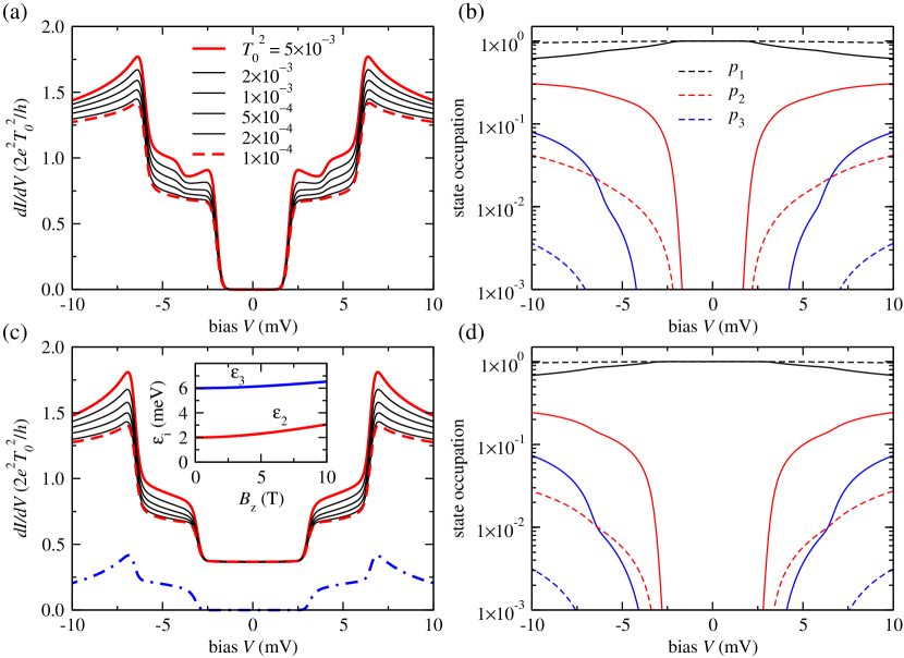
Figure 12: Tunneling spectra of a spin $S=1$ system at different coupling strengths $T_{0}^{2}$ between tip and sample. The simulation parameters are identical to the ones used in figure 8: $g=2$, $D=-5$ meV, $E=1$ meV, $U=0$, $J\rho_{s}=-0.1$, $T=1$ K. (a) Normalized zero field spectra for $T_{0}^{2}$ ranging from $1\times 10^{-4}$ (dashed red line) to $5\times 10^{-3}$ (full red line). At increased $T_{0}$ a feature at $eV=\pm|\epsilon_{3}-\epsilon_{2}|\approx\pm 4$ meV appears and the apparent strength of the peaks at $eV=\pm\epsilon_{3}$ increase. (b) State occupancy in steady-state for the smallest (dashed lines) and highest (full lines) coupling strengths. (c) and (d) Same as (a) and (b) but at an applied field of $B_{z}=10$ T. The dashed-dotted line in (c) is the relative difference between the spectra at highest and lowest coupling strength. The inset in (c) shows the evaluation of the state energy $\epsilon_{i}$ with field.

The coupling constants correspond to a tunneling resistance between $R_{T}\approx 130$ M$\Omega$ and $\approx 2.6$ M$\Omega$, which is equivalent to a tunneling current of $I\approx 150$ pA – $8$ nA at a bias of $V=20$ mV. Note, that these are quite typical parameters for STM experiments.

Without magnetic field and at small couplings we observe a spectrum which does not differ significantly from the one calculated in the zero-current approximation. The average occupation of the two excited states increases only slowly for voltages above the threshold for these transitions and reaches at $V=\pm 10$ mV only about $4\%$ for $p_{2}$ and less than $0.4\%$ for $p_{3}$ (dashed lines in figure 12b). This situation changes when the tip-sample coupling is increased. At larger $T_{0}$ an additional feature appears in the spectrum at about $\pm 4$ mV, which is due to transitions from the state $\left|\psi_{2}\right\rangle$ to $\left|\psi_{3}\right\rangle$. These transitions are only possible because the probabilities $p_{i}$ are driven far from thermal equilibrium and $p_{2}$ has already a significant weight at $|V|=4$ mV. Similar current induced pumping to higher excitation states has been observed for example for Mn-dimers adsorbed on Cu₂N [13], for small Fe clusters containing only a few atoms on Cu(111) [2], or for Fe-OEP-Cl (Fe-octaethylporphyrin-chloride) molecules adsorbed on Pb(111) [115]. Interestingly, the latter experiment was performed on a superconducting surface and with a superconducting Pb-tip which made it necessary to account for the gap around the Fermi energy in the quasi-particle density of states of tip and sample.

If we now add a magnetic field of $B_{z}=10$ T to our simulation , the situation changes: The energy differences $\epsilon_{12}$ and $\epsilon_{23}$ between the first and second, and second and third eigenstate, respectively, are almost identical (see figure 12c inset) masking the additional step-like feature when pumping into energetically higher states. Nevertheless, also here a clear change of the spectrum occurs at high tip-sample couplings. We observe an increased relative conductance between $\epsilon_{2}$ and $\epsilon_{3}$ and a stronger third order peak at $eV=\pm\epsilon_{3}$. This feature is mainly due to the third order scattering process $(232)$ now possible, as apparently visible when taking the relative difference between the spectra at strongest and weakest coupling strength (dashed dotted line in figure 12c).

As long as the tip is not spin-polarized, the current induced pumping into higher states cannot lead to an inversion of the state occupancy. The state’s lifetime $\tau_{i}$ for the eigenstate $\left|\psi_{i}\right\rangle$ is inversely proportional to the sum of all scattering processes which leaves the state:

$$\tau_{i}^{-1}=\sum_{j\neq i}\left(\Gamma_{ij}^{\rm t\rightarrow s}(eV)+\Gamma_{ij}^{\rm s\rightarrow t}(eV)+\Gamma_{ij}^{\rm s\rightarrow,s}(eV)\right).$$ (42)

While for spin-averaged electrodes the scattering matrix elements do not change when inverting the initial and final state, the energetically higher states must have always a shorter lifetime.

This behavior changes drastically when a spin-polarized tip is used. We have seen that, in particular for spin systems with a potential scattering $U=S/2$, the tunneling conductance and thereby the scattering rate depends strongly on the bias polarity (Figure 4). Experimentally, this was first detected for Mn adatoms adsorbed on Cu₂N [13] and successfully discussed theoretically in a second order perturbative scattering model [80, 79]. Figure 13 shows the simulated spectra of a Mn spin system at high field which – due to the small magnetic anisotropy – leads to an almost equidistant energy difference between the five eigenstates.

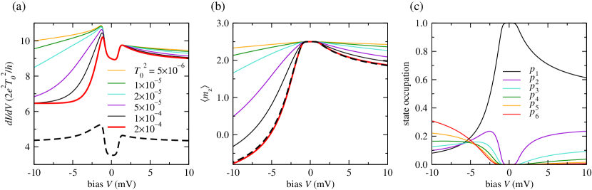
Figure 13: Simulated tunneling spectra of a Mn atom on Cu₂N with spin $S=5/2$ at different coupling strengths $T_{0}^{2}$ between tip and sample and at a magnetic field of $B_{z}=7$ T. Simulation parameters are $g=1.9$, $D=-40\ \mu$eV, $E=0$, $U=1.3$, $J\rho_{s}=-0.02$, $T=1$ K, and a tip polarization of $\eta^{\rm t}=0.3$. (a) Normalized spectra, and (b) averaged magnetic moment $\left\langle m_{z}\right\rangle$ in units of $\hbar$ for $T_{0}^{2}$ ranging from $5\times 10^{-6}$ to $2\times 10^{-4}$, corresponding to a tunneling resistance of $R_{T}\approx 270$ M$\Omega$ to $\approx 6.8$ M$\Omega$ or a stabilization current of $I\approx 35$ pA – $1.5$ nA at a bias of $eV=+10$ meV. The dashed lines in (a) and (b) are calculated with $U=0$ at $T_{0}^{2}=2\times 10^{-4}$. (c) Occupancy of the six eigenstates at steady-state conditions for $T_{0}^{2}=2\times 10^{-4}$.

These eigenstates are well described by pure states with the magnetic quantum numbers $m_{z}=-5/2,-3/2,...,+5/2$.

At low tip sample couplings the $dI/dV$ spectrum is similar to the ones simulated without rate-equations (Figure 9d and e), but at higher coupling we observe a drastic reduction of the differential conductance at negative bias. This decrease is concomitant with the reduction of the average magnetization $\langle m_{z}\rangle=\tr\left(\hat{S}_{z}\sum_{i}p_{i}\left|\psi_{i}\right\rangle\left\langle\psi_{i}\right|\right)$. For the highest $T_{0}$ the average magnetization becomes even negative at negative bias showing clearly the inversion of the state populations. Interestingly, the strong bias asymmetry in the $dI/dV$ spectrum is only due to the potential scattering. Simulating the system with $U=0$ results in a much less asymmetric spectrum, even though the bias dependence of the state populations and average magnetization are unaltered.

Finally, we have to remark that experimentally an effective interaction of the substrate conduction electrons with the Mn spin of $G_{S}=2.7\ \mu$S was found [13]. This is much higher than the spin-substrate scattering determined solely by the spectroscopically estimated $J\rho_{0}\approx-0.02$ which results to $G_{S}=2e^{2}/h\times(J\rho_{s})^{2}S(S+1)\approx 0.3\ \mu$S. This means that in this particular system roughly 90% of the spin relaxations with the substrate electrons must originate from scattering processes which do not directly leave their fingerprint in the observable differential conductance spectrum. In this context, ab-inito density functional calculations have found an about $3.1$ times higher coupling to the substrate via the $3d_{xz}$ and $3d_{x^{2}-y^{2}}$ orbitals than experimentally observed [116], while the approach discussed here neglect any orbital symmetry.

5.1 Current induced correlations

Comparing the dynamical model outlined above with experimental data that require the evaluation up to third order scattering is a very intriguing test of the capability, as well as the limitations, of this approach. Thus, we will now analyze spectroscopic data that have been measured for Fe adatoms on Cu₂N using spin-averaged and spin-polarized tips [99]. Figure 14 shows the experimental data obtained for two different magnetic field directions;

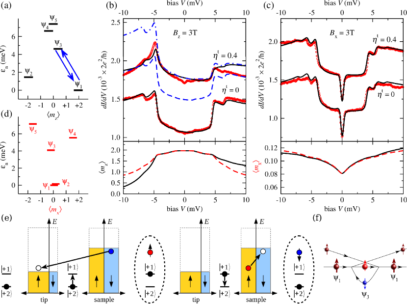
Figure 14: Correlations induced by tunneling substrate electrons. (a) Schematic state diagram for an Fe atom on Cu₂N at $B_{z}=3$ T. The blue arrows illustrate the third order transition (131). (b) and (c) Top panels: Experimental data from reference [99] of a Fe atom on Cu₂N measured with a spin averaging tip ($\eta^{\rm t}=0$) and a spin polarized tip ($\eta^{\rm t}\approx 0.4$) at applied field in $z$ (a) and $x$ (b) direction (colored circles). The best fits (full lines) results in $g=2.11$, $D=-1.6$ meV, $E=0.31$ meV, $U=0.35$, $J\rho_{s}=-0.1$, $T_{\rm eff}=1$ K, and $T_{0}^{2}=3.2\times 10^{-4}$. Spectra obtained and simulated with spin-polarized tips are shifted vertically by $0.5\times 10^{-3}(2e^{2}/h)$. The dashed (dotted dashed) line in (b) is calculated with $U=0$ (in zero-current approximation). Bottom panels: Corresponding average magnetic moment in field direction in units of $\hbar$ (full lines: spin-polarized tip, dashed lines: spin-average tip). (d) Schematic state diagram for an Fe atom at $B_{x}=3$ T. (e) and (f) Schematic illustration (e) and Feyman-like diagram (f) of the third order scattering process (131) which leads to the peak at $V\approx-5$ mV in panel (a).

along the main anisotropy axis (easy axis, $B_{z}$) which leads to a strong polarization of the eigenstates along the magnetic field (Figure 14a) and, perpendicular to it, along the hard axis ($B_{x}$) which produces only a small polarization of the lowest eigenstates (Figure 14d).

In this experiment the spin polarization was deliberately changed by vertical manipulation (”picking-up“) [117, 13] of a Mn atom onto the apex of the tip, changing its polarization from $\eta^{\rm t}\approx 0$ to $\eta^{\rm t}\approx 0.4$ and enabling the study of the identical atom with and without a polarized tip. The experimental data for the spin-average and for the spin-polarized measurements along the hard axis can be well simulated within one set of parameters (figure 14c). Surprisingly, the spectra are almost identical to simulations using only the zero-current approximation. Thus, the moderate coupling between tip and sample does not disturb significantly the state populations. This is also evident by plotting the average magnetic moment along the applied field (lower panels in figure 14b and c). The small magnetic field (compared to the anisotropy energy) of only $B_{x}=3$ T along the magnetically hard-axis cannot polarize the Fe atom significantly (Figure 14d). This means, that the spin imbalance produced by a spin-polarized current has only little influence on the $dI/dV$ spectrum. However, note that the small shift towards higher energies of the step at $|V|\approx 4$ mV, which has its origin in transitions between the states $\left|\psi_{1}\right\rangle$ and $\left|\psi_{3}\right\rangle$, might be due to an interaction between the spin system on the surface and the spin polarized electrode of the tip [118, 119].

The situation changes quite drastically when the magnetic field is applied along the easy axis and the spectrum is taken with the spin-polarized tip (Figure 14b). A strong peak at $V\approx-5$ mV appears concomitant with the apparent disappearance of the step at precisely the same energy, that was clearly visible in the spectrum measured with the spin-averaging tip. Fortunately, the model describes this spectrum quite well, too and thus allows us to discuss the physical origin of these differences.

Comparing the spectrum with the one calculated in the zero-current-approximation reveals that the disappearance of the step is indeed due to the increased coupling between tip and sample. The origin lies in the finite $U$, quite similar to the differential conductance reduction observed at negative bias for the Mn system (Figure 13). Indeed, we see that the spectrum calculated with the same set of parameters except $U=0$ leads to a spectrum in which the step-like increase of the $dI/dV$ at $V<-4$ mV is maintained. Furthermore, we notice that the calculated magnetization $\left\langle m_{z}\right\rangle$ decreased abruptly below this tunneling bias voltage, much faster than for the spin-averaging tip, due to the increased population of the states $\left|\psi_{2}\right\rangle$ and $\left|\psi_{3}\right\rangle$ (Figure 14b lower panel).

While the effects discussed above give a plausible explanation for the overall shape of the spectrum, there is still a noticeable discrepancy between experiment and simulation. In particular, the experimental $dI/dV$ data show a significantly stronger peak at $V\approx-5$ mV than one would expect based on the simulation, resembling of the effects of strong correlations discussed in section 4 (which are not covered by the model). Thus, it is worth to dissect the characteristic peak which has its origin in the third order process (131) in which the spin system is scattered from $\left|\psi_{1}\right\rangle\rightarrow\left|\psi_{3}\right\rangle\rightarrow\left|\psi_{1}\right\rangle$. With the spin-polarized tip this transition has a significantly higher probability to occur when the electrons tunnel from sample to tip. The process is illustrated in figures 14d and 14f. It starts with an $\left|\downarrow\right\rangle$ electron in the sample which scatters on the spin system changing its grounstate from $\left|\psi_{1}\right\rangle$ to $\left|\psi_{3}\right\rangle$ and then tunnels, with increased probability, as $\left|\uparrow\right\rangle$ electron into the majority states of the tip. The spin-down hole in the sample will lead to a slightly higher spin-up electron density close to the Fe atom. Next, a $\left|\uparrow\right\rangle$ electron from the sample fills the $\left|\downarrow\right\rangle$ hole together with changing the localized spin-state from $\left|\psi_{3}\right\rangle$ back to $\left|\psi_{1}\right\rangle$ (Figure 14d). During this process the substrate electrons are correlated with the spin state. While the magnetic moment for $\left|\psi_{1}\right\rangle$ is approximately $m_{z}\approx+2$ and for $\left|\psi_{3}\right\rangle$ $m_{z}\approx+1$, respectively, at low enough temperature and at sufficiently negative bias and tunneling current, a correlated out-of-equilibrium Kondo-state develops which has the total wavefunction

$$\Psi^{total}=\frac{1}{\sqrt{2}}\left(\left|\downarrow^{\rm s}\right\rangle\left|+2\right\rangle-\left|\uparrow^{\rm s}\right\rangle\left|+1\right\rangle\right).$$ (43)

Even though the experimental data only give hints that this correlated state has formed, a similar non-equilibrium Kondo formation has been found in transport measurements on carbon nanotubes [120]. The physical properties of such a non-equilibrium correlated state are very intriguing [121, 122]. Entering this state, the substrate electrons partly screen the magnetic moment of the Fe spin reducing it to $S-1/2$. Such an underscreened Kondo state should show a very particular temperature and energy dependence [123, 124, 125, 126]. Interestingly, in a system like the one discussed here, the transition between weak and strong coupling is not only governed by a characteristic temperature $T_{K}$ [127], but the formation of this correlated state is deliberately tuned by drastically increasing the probability of its creation when applying a spin-polarized current of sufficient energy by the probing tip. This enables us to envision for example pump-probe experiments [14] in which the time-evolution of the formation and the decay of this correlated state is measured in detail.

6 Summary

In this manuscript I have shown that applying perturbation theory to quantum spin systems enables one to describe experimentally measured differential conductance spectra with very high accuracy. This enables one to obtain a profound understanding of the physical processes on play and to separate single- as well as many-electron effects.

The versatility of low-temperature scanning tunneling measurements on single and complexly coupled spin systems led me to believe that we should expect a multitude of exciting new experiments for the future, which will further deepening our fundamental knowledge on quantum systems in general and, in particular, quantum magnetism. Perturbative models, like the one outlined here, might be of help in such systems. For that, the supplemental material to this manuscript include an easy usable software package that allows not only to simulate the differential conductance spectra of arbitrary complex spin systems, but additionally allows one to fit experimental data to the model.

In this manuscript we have restricted ourselves to the adiabatic limit and neglected any time dependence in the parameters. However, it is straightforward to expand this model to capture also time dependent pump-probe measurements. In such a framework, coherent state superpositions could be accounted for by using, for example, a Bloch-Redfield approach in which the spin system is coupled to an open quantum-system [128, 114, 129] and in which interactions up to third order are included to account not only for the decay but also for the creation of coherences.

Additionally, the study of the coupling between the spin-system and other (quasi)-particles, like phonons, photons, or magnons would be very interesting. Furthermore, while the perturbative approach fails when the system enters the strong-coupling Kondo-regime, it would be very intriguing to combine the simple model outlined here, with exact quantum impurity models.

Appendix A Matrix elements for arbitrary spin polarization

The two arbitrary spin density matrices $\varrho^{\rm t}$ and $\varrho^{\rm s}$ are a full description of the ensemble states in the tip and sample electron bath close to the Fermi energy. The eigenvectors $\left|\varphi_{i}^{\rm t}\right\rangle$ and $\left|\varphi_{i}^{\rm s}\right\rangle$ of $\varrho^{\rm t}$ and $\varrho^{\rm s}$ are representative eigenstates of these incoherent ensembles and enables one to calculate the interaction transition intensities between them as:

$$\xi^{x,y,z,I}_{i^{\prime}f^{\prime}}=\sqrt{\lambda_{i^{\prime}}^{\rm t}\lambda_{f^{\prime}}^{\rm s}}\left\langle\varphi_{f^{\prime}}^{\rm s}\right|\hat{\sigma}_{x,y,z,I}\left|\varphi_{i^{\prime}}^{\rm t}\right\rangle,$$ (44)

with $\lambda_{i}^{\rm t}$ and $\lambda_{i}^{\rm s}$ as the eigenvalues of the corresponding eigenvectors. Note, that due to the in general incoherent spin ensembles in tip and sample equation 44 has to be evaluated independently for all combinations of $i^{\prime}=1,2$ and $f^{\prime}=1,2$.

For the localized spin system we can write similarly the transition intensities between the eigenstates:

$$\Xi_{if}^{x,y,z}=\left\langle\psi_{f}\right|\hat{S}_{x,y,z}\left|\psi_{i}\right\rangle,$$ (45)

so that the absolute square of the matrix element in equation 13 calculates to:

$$\left|\mathcal{M}_{(1)if}^{\rm t\rightarrow s}\right|^{2}=\sum_{i^{\prime},f^{\prime}}\left|\frac{1}{2}\left(\xi^{x}_{i^{\prime}f^{\prime}}\Xi^{x}_{if}+\xi^{y}_{i^{\prime}f^{\prime}}\Xi^{y}_{if}+\xi^{z}_{i^{\prime}f^{\prime}}\Xi^{z}_{if}\right)+U\xi^{I}_{i^{\prime}f^{\prime}}\delta_{if}\right|^{2}.$$ (46)

The interference term between $\mathcal{M}_{1}$ and $\mathcal{M}_{2}$ (equation 23) can be evaluated in an analogous way leading to:

$$M_{fi}\tilde{M}_{mf}M_{im}=\sum_{\genfrac{}{}{0.0pt}{}{j,k,l=}{\{x,y,z,I\}}}\,\sum_{i^{\prime},m^{\prime},f^{\prime}}\bar{\xi}^{l}_{f^{\prime}i^{\prime}}\Xi^{l}_{fi}\times\tilde{\xi}^{k}_{m^{\prime}f^{\prime}}\Xi^{k}_{mf}\times\xi^{j}_{i^{\prime}m^{\prime}}\Xi^{j}_{im},$$ (47)

and for the reversed order processes:

$$M_{fi}M_{mf}\tilde{M}_{im}=\sum_{\genfrac{}{}{0.0pt}{}{j,k,l=}{\{x,y,z,I\}}}\,\sum_{i^{\prime},m^{\prime},f^{\prime}}\bar{\xi}^{l}_{f^{\prime}i^{\prime}}\Xi^{l}_{fi}\times\xi^{k}_{m^{\prime}f^{\prime}}\Xi^{k}_{mf}\times\tilde{\xi}^{j}_{i^{\prime}m^{\prime}}\Xi^{j}_{im}.$$ (48)

The tilde ($\tilde{\xi}$) and bar ($\bar{\xi}=\xi^{\dagger}$) account for processes which starts and ends in the sample, and for processes in which tunneling electrons traverse the junction in the opposite direction, i. e. which starts in the sample and ends in the tip, respectively. They can be calculated in an analogous way with equation 44.

References

References

- [1] S. Loth, S. Baumann, C. P. Lutz, D. M. Eigler, and A. J. Heinrich. Bistability in atomic-scale antiferromagnets. Science, 335:196, 2012.
- [2] A. A. Khajetoorians, B. Baxevanis, C. Hübner, T. Schlenk, S. Krause, T. O. Wehling, S. Lounis, A. Lichtenstein, D. Pfannkuche, J. Wiebe, and R. Wiesendanger. Current-driven spin dynamics of artificially constructed quantum magnets. Science, 339:55, 2013.
- [3] F. Delgado, S. Loth, M. Zielinski, and J. Fernández-Rossier. The emergence of classical behavior in magnetic adatoms. Europhys. Lett., 109:57001, 2015.
- [4] A. A. Khajetoorians, J. Wiebe, B. Chilian, and R. Wiesendanger. Realizing all-spin–based logic operations atom by atom. Science, 332:1062, 2011.
- [5] M. N. Leuenberger and D. Loss. Quantum computing in molecular magnets. Nature, 410:789, 2001.
- [6] A. J. Heinrich, J. A. Gupta, C. P. Lutz, and D. M. Eigler. Single-atom spin-flip spectroscopy. Science, 306:466, 2004.
- [7] C. F. Hirjibehedin, C. P. Lutz, and A. J. Heinrich. Spin coupling in engineered atomic structures. Science, 312:1021, 2006.
- [8] C. F. Hirjibehedin, C. Y. Lin, A. F. Otte, M. Ternes, C. P. Lutz, B. A. Jones, and A. J. Heinrich. Large magnetic anisotropy of a single atomic spin embedded in a surface molecular network. Science, 317:1199, 2007.
- [9] A. F. Otte, M. Ternes, S. Loth, K. von Bergmann, H. Brune, C. P. Lutz, C. F. Hirjibehedin, and A. J. Heinrich. The role of magnetic anisotropy in the Kondo effect. Nature Physics, 4:847, 2008.
- [10] A. F. Otte, M. Ternes, S. Loth, C. P. Lutz, C. F. Hirjibehedin, and A. J. Heinrich. Spin excitations of a Kondo-screened atom coupled to a second magnetic atom. Phys. Rev. Lett., 103:107203, 2009.
- [11] T. Choi, C. D. Ruggiero, and J. A. Gupta. Tunneling spectroscopy of ultrathin insulating Cu2N films, and single Co adatoms. J. Vac. Sci. Technol. B, 27:887, 2009.
- [12] M. Ternes, A. J. Heinrich, and W. D. Schneider. Spectroscopic manifestations of the Kondo effect on single adatoms. J. Phys.: Condens. Matter, 21:053001, 2009.
- [13] S. Loth, K. von Bergmann, M. Ternes, A. F. Otte, C. P. Lutz, and A. J. Heinrich. Controlling the state of quantum spins with electric currents. Nature Physics, 6:340, 2010.
- [14] S. Loth, M. Etzkorn, C. P. Lutz, D. M. Eigler, and A. J. Heinrich. Measurement of fast electron spin relaxation times with atomic resolution. Science, 329:1628, 2010.
- [15] B. Bryant, A. Spinelli, J. J. T. Wagenaar, M. Gerrits, and A. F. Otte. Local control of single atom magnetocrystalline anisotropy. Phys. Rev. Lett., 111:127203, 2013.
- [16] J. C. Oberg, M. R. Calvo, F. Delgado, M. Moro-Lagares, D. Serrate, D. Jacob, J. Fernández-Rossier, and C. F. Hirjibehedin. Control of single-spin magnetic anisotropy by exchange coupling. Nature Nanotechnology, 9:64, 2013.
- [17] T. Choi, M. Badal, S. Loth, J.-W. Yoo, C. P. Lutz, A. J. Heinrich, A. J. Epstein, D. G. Stroud, and J. A. Gupta. Magnetism in single metalloorganic complexes formed by atom manipulation. Nano Lett., 14:1196, 2014.
- [18] K. von Bergmann, M. Ternes, S. Loth, C. P. Lutz, and A. J. Heinrich. Spin-polarization of the split Kondo state. Phys. Rev. Lett., 114:076601, 2015.
- [19] A. Spinelli, B. Bryant, F. Delgado, J. Fernández-Rossier, and A. F. Otte. Imaging of spin waves in atomically designed nanomagnets. Nature Materials, 13:782, 2014.
- [20] A. Spinelli, M. Gerrits, R. Toskovic, B. Bryant, M. Ternes, and A. F. Otte. Full experimental realisation of the two-impurity Kondo problem. cond-mat.mes-hall, page arXiv:1411.4415, 2014.
- [21] S. Kahle, Z. Deng, N. Malinowski, C. Tonnoir, A. Forment-Aliaga, N. Thontasen, G. Rinke, D. Le, V. Turkowski, T. S. Rahman, S. Rauschenbach, M. Ternes, and K. Kern. The quantum magnetism of individual manganese-12-acetate molecular magnets anchored at surfaces. Nano Lett., 12:518, 2012.
- [22] Y. Zhang, S. Kahle, T. Herden, C. Stroh, M. Mayor, U. Schlickum, M. Ternes, P. Wahl, and K. Kern. Temperature and magnetic field dependence of a Kondo system in the weak coupling regime. Nature Comm., 4:2110, 2013.
- [23] P. Gambardella, S. Rusponi, M. Veronese, S. S. Dhesi, C. Grazioli, A. Dallmayer, I. Cabria, R. Zeller, P. H. Dederichs, K. Kern, C. Carbone, and H. Brune. Giant magnetic anisotropy of single cobalt atoms and nanoparticles. Science, 300:1130, 2003.
- [24] D. Gatteschi, R. Sessoli, and D. Villani. Molecular Nanomagnets. Oxford University Press, 2006.
- [25] D. Dai, H. Xiang, and M.-H. Whangbo. Effects of spin-orbit coupling on magnetic properties of discrete and extended magnetic systems. J. Comp. Chem., 29:2187, 2008.
- [26] I. G. Rau, S. Baumann, S. Rusponi, F. Donati, S. Stepanow, L. Gragnaniello, J. Dreiser, C. Piamonteze, F. Nolting, S. Gangopadhyay, O. R. Albertini, R. M. MacFarlane, C. P. Lutz, B. A. Jones, P. Gambardella, A. J. Heinrich, and H. Brune. Reaching the magnetic anisotropy limit of a metal atom. Science, 344:988, 2014.
- [27] A. J. Heinrich, C. P. Lutz, J. A. Gupta, and D. M. Eigler. Molecule cascades. Science, 298:1381, 2002.
- [28] J. A. Gupta, C. P. Lutz, A. J. Heinrich, and D. M. Eigler. Strongly coverage-dependent excitations of adsorbed molecular hydrogen. Phys. Rev. B, 71:115416, 2005.
- [29] M. Pivetta, M. Ternes, F. Patthey, and W. D. Schneider. Diatomic molecular switches to enable the observation of very-low-energy vibrations. Phys. Rev. Lett., 99:126104, 2007.
- [30] W. A. Hofer, G. Teobaldi, and N. Lorente. Creating pseudo-Kondo resonances by field-induced diffusion of atomic hydrogen. Nanotechnology, 19:305701, 2008.
- [31] F. D. Natterer, F. Patthey, and H. Brune. Distinction of nuclear spin states with the scanning tunneling microscope. Phys. Rev. Lett., 111:175303, 2013.
- [32] I. Fernandez-Torrente, K. J. Franke, and J. I. Pascual. Vibrational Kondo effect in pure organic charge-transfer assemblies. Phys. Rev. Lett., 101:217203, 2008.
- [33] F. May, M. R. Wegewijs, and W. Hofstetter. Interaction of spin and vibrations in transport through single-molecule magnets. Beilstein J. Nanotechnol., 2:693, 2011.
- [34] J. Kondo. Resistance minimum in dilute magnetic alloys. Prog. Theor. Phys., 32:37, 1964.
- [35] J. Kondo. Effect of ordinary scattering on exchange scattering from magnetic impurity in metals. Phys. Rev., 169:437, 1968.
- [36] A. C. Hewson. The Kondo Problem to Heavy Fermions. Cambridge University Press, Cambridge, 1997.
- [37] J. T. Li, W. D. Schneider, R. Berndt, and B. Delley. Kondo scattering observed at a single magnetic impurity. Phys. Rev. Lett., 80:2893, 1998.
- [38] V. Madhavan, W. Chen, T. Jamneala, M. F. Crommie, and N. S. Wingreen. Tunneling into a single magnetic atom: Spectroscopic evidence of the Kondo resonance. Science, 280:567, 1998.
- [39] H. C. Manoharan, C. P. Lutz, and D. M. Eigler. Quantum mirages formed by coherent projection of electronic structure. Nature, 403:512, 2000.
- [40] V. Madhavan, W. Chen, T. Jamneala, M. F. Crommie, and N. S. Wingreen. Local spectroscopy of a Kondo impurity: Co on Au(111). Phys. Rev. B, 64:165412, 2001.
- [41] K. Nagaoka, T. Jamneala, M. Grobis, and M. F. Crommie. Temperature dependence of a single Kondo impurity. Phys. Rev. Lett., 88:077205, 2002.
- [42] N. Knorr, M. A. Schneider, L. Diekhoner, P. Wahl, and K. Kern. Kondo effect of single Co adatoms on Cu surfaces. Phys. Rev. Lett., 88:096804, 2002.
- [43] M. A. Schneider, L. Vitali, N. Knorr, and K. Kern. Observing the scattering phase shift of isolated Kondo impurities at surfaces. Phys. Rev. B, 65:121406, 2002.
- [44] P. Wahl, L. Diekhoner, M. A. Schneider, L. Vitali, G. Wittich, and K. Kern. Kondo temperature of magnetic impurities at surfaces. Phys. Rev. Lett., 93:176603, 2004.
- [45] L. Limot and R. Berndt. Kondo effect and surface-state electrons. Appl. Surf. Sci., 237:576, 2004.
- [46] P. Wahl, L. Diekhoner, G. Wittich, L. Vitali, M. A. Schneider, and K. Kern. Kondo effect of molecular complexes at surfaces: Ligand control of the local spin coupling. Phys. Rev. Lett., 95:166601, 2005.
- [47] U. Fano. Effects of configuration interaction on intensities and phase shifts. Phys. Rev., 124:1866, 1961.
- [48] O. Ujsaghy, J. Kroha, L. Szunyogh, and A. Zawadowski. Theory of the Fano resonance in the STM tunneling density of states due to a single Kondo impurity. Phys. Rev. Lett., 85:2557, 2000.
- [49] A. Kiss, Y. Kuramoto, and S. Hoshino. Numerical study of Kondo impurity models with strong potential scattering: Reverse Kondo effect and antiresonance. Phys. Rev. B, 84:174402, 2011.
- [50] J. Ren, H. Guo, J. Pan, Y. Y. Zhang, X. Wu, H.-G. Luo, S. Du, S. T. Pantelides, and H.-J. Gao. Kondo effect of cobalt adatoms on a graphene monolayer controlled by substrate-induced ripples. Nano Lett., 14:4011, 2014.
- [51] P. Jacobson, T. Herden, M. Muenks, Laskin G., O. O. Brovko, V. S. Stepanyuk, M. Ternes, and K. Kern. Quantum engineering of spin and anisotropy in magnetic molecular junctions. cond-mat.mes-hall, page arXiv:1505.02277, 2015.
- [52] A. A. Khajetoorians, B. Chilian, J. Wiebe, S. Schuwalow, F. Lechermann, and R. Wiesendanger. Detecting excitation and magnetization of individual dopants in a semiconductor. Nature, 467:1084, 2010.
- [53] B. Chilian, A. A. Khajetoorians, J. Wiebe, and R. Wiesendanger. Experimental variation and theoretical analysis of the inelastic contribution to atomic spin excitation spectroscopy. Phys. Rev. B, 83:195431, 2011.
- [54] F. Donati, Q. Dubout, F. Autés, Patthey, F. Calleja, P. Gambadella, O. V. Yazyev, and H. Brune. Magnetic moment and anisotropy of individual Co atoms on graphene. Phys. Rev. Lett., 111:236801, 2013.
- [55] T. Balashov, T. Schuh, A. F. Takács, A. Ernst, S. Ostanin, J. Henk, I. Mertig, P. Bruno, T. Miyamachi, S. Suga, and W. Wulfhekel. Magnetic anisotropy and magnetization dynamics of individual atoms and clusters of Fe and Co on Pt(111). Phys. Rev. Lett., 102:257203, 2009.
- [56] A. A. Khajetoorians, T. Schlenk, B. Schweflinghaus, M. dos Santos Dias, M. Steinbrecher, M. Bouhassoune, S. Lounis, J. Wiebe, and R. Wiesendanger. Spin excitations of individual Fe atoms on Pt(111): Impact of the site-dependent giant substrate polarization. Phys. Rev. Lett., 111:157204, 2013.
- [57] T. Balashov, T. Miyamachi, T. Schuh, T. Märkl, C. Bresch, and W. Wulfhekel. Dynamic magnetic excitations in 3d and 4f atoms and clusters. Surf. Sci., 630:331, 2014.
- [58] A. A. Khajetoorians, S. Lounis, B. Chilian, A. T. Costa, L. Zhou, D. L. Mills, J. Wiebe, and R. Wiesendanger. Itinerant nature of atom-magnetization excitation by tunneling electrons. Phys. Rev. Lett., 106:037205, 2011.
- [59] B. Chilian, A. A. Khajetoorians, S. Lounis, A. T. Costa, D. L. Mills, J. Wiebe, and R. Wiesendanger. Anomalously large g factor of single atoms adsorbed on a metal substrate. Phys. Rev. B, 84:212401, 2011.
- [60] T. Schuh, T. Miyamachi, S. Gerstl, M. Geilhufe, M. Hoffmann, S. Ostanin, W. Hergert, A. Ernst, and W. Wulfhekel. Magnetic excitations of rare earth atoms and clusters on metallic surfaces. Nano Lett., 12:4805, 2012.
- [61] T. Miyamachi, T. Schuh, T. Märkl, C. Bresch, T. Balashov, A. Stöhr, C. Karlewski, S. Andre, M. Marthaler, M. Hoffmann, M. Geilhufe, S. Ostanin, W. Hergert, I. Mertig, G. Schön, A. Ernst, and W. Wulfhekel. Stabilizing the magnetic moment of single holmium atoms by symmetry. Nature, 503:242, 2013.
- [62] B. N. Harmon and A. J. Freeman. Spin-polarized energy-band structure, conduction-electron polarization, spin densities, and the neutron magnetic form factor of ferromagnetic gadolinium. Phys. Rev. B, 10:1979, 1974.
- [63] A. Zhao, Q. Li, L. Chen, H. Xiang, W. Wang, S. Pan, B. Wang, X. Xiao, J. Yang, J. G. Hou, and Q. Zhu. Controlling the Kondo effect of an adsorbed magnetic ion through its chemical bonding. Science, 309:1542, 2005.
- [64] X. Chen, Y. S. Fu, S.-H. Ji, T. Zhang, P. Cheng, X. C. Ma, X.-L. Zou, W. H. Duan, J. F. Jia, and Q. K. Xue. Probing superexchange interaction in molecular magnets by spin-flip spectroscopy and microscopy. Phys. Rev. Lett., 101:197208, 2008.
- [65] N. Tsukahara, K. Noto, M. Ohara, S. Shiraki, N. Takagi, Y. Takata, J. Miyawaki, M. Taguchi, A. Chainani, S. Shin, and M. Kawai. Adsorption-induced switching of magnetic anisotropy in a single iron(II) phthalocyanine molecule on oxidized Cu(110) surface. Phys. Rev. Lett., 102:167203, 2009.
- [66] S.-H. Ji, Y. S. Fu, T. Zhang, X. Chen, J. F. Jia, Q.-K. Xue, and X.-C. Ma. Kondo effect in self-assembled manganese phthalocyanine monolayer on Pb islands. Chin. Phys. Lett., 27:087202, 2010.
- [67] K. J. Franke, G. Schulze, and J. I. Pascual. Competition of superconducting phenomena and Kondo screening at the nanoscale. Science, 332:940, 2011.
- [68] N. Tsukahara, S. Shiraki, S. Itou, N. Ohta, N. Takagi, and M. Kawai. Evolution of Kondo resonance from a single impurity molecule to the two-dimensional lattice. Phys. Rev. Lett., 106:187201, 2011.
- [69] E. Minamitani, N. Tsukahara, D. Matsunaka, Y. Kim, N. Takagi, and M. Kawai. Symmetry-driven novel Kondo effect in a molecule. Phys. Rev. Lett., 109:086602, 2012.
- [70] L. Liu, K. Yang, Y. Jiang, B. Song, W. Xiao, L. Li, H. Zhao, Y. Wang, S. Du, M. Ouyang, W. A. Hofer, A. H. Castro Neto, and H. J. Gao. Reversible single spin control of individual magnetic molecule by hydrogen atom adsorption. Sci. Rep., 3:1210, 2013.
- [71] Y. S. Fu, T. Zhang, S.-H. Ji, X. Chen, X.-C. Ma, J.-F. Jia, and Q.-K. Xue. Identifying charge states of molecules with spin-flip spectroscopy. Phys. Rev. Lett., 103:257202, 2009.
- [72] B. W. Heinrich, G. Ahmadi, V. L. Müller, L. Braun, J. I. Pascual, and K. J. Franke. Change of the magnetic coupling of a metal–organic complex with the substrate by a stepwise ligand reaction. Nano Lett., 13:4840, 2013.
- [73] J. Bauer, J. I. Pascual, and K. J. Franke. Microscopic resolution of the interplay of Kondo screening and superconducting pairing: Mn-phthalocyanine molecules adsorbed on superconducting Pb(111). Phys. Rev. B, 87:075125, 2013.
- [74] M. Persson. Theory of inelastic electron tunneling from a localized spin in the impulsive approximation. Phys. Rev. Lett., 103:050801, 2009.
- [75] N. Lorente and J. P. Gauyacq. Efficient spin transitions in inelastic electron tunneling spectroscopy. Phys. Rev. Lett., 103:176601, 2009.
- [76] J. P. Gauyacq, F. D. Novaes, and N. Lorente. Magnetic transitions induced by tunneling electrons in individual adsorbed -phthalocyanine molecules (Fe and Co). Phys. Rev. B, 81:165423, 2010.
- [77] A. Hurley, N. Baadji, and S. Sanvito. Spin-flip inelastic electron tunneling spectroscopy in atomic chains. Phys. Rev. B, 84:035427, 2011.
- [78] J. Fransson, O. Eriksson, and A. V. Balatsky. Theory of spin-polarized scanning tunneling microscopy applied to local spins. Phys. Rev. B, 81:115454, 2010.
- [79] F. Delgado and J. Fernández-Rossier. Spin dynamics of current-driven single magnetic adatoms and molecules. Phys. Rev. B, 82:134414, 2010.
- [80] F. Delgado, J. J. Palacios, and J. Fernández-Rossier. Spin-transfer torque on a single magnetic adatom. Phys. Rev. Lett., 104:026601, 2010.
- [81] A. Hurley, A. Narayan, and S. Sanvito. Spin-pumping and inelastic electron tunneling spectroscopy in topological insulators. Phys. Rev. B, 87:245410, 2013.
- [82] F. Delgado and J. Fernández-Rossier. Cotunneling theory of atomic spin inelastic electron tunneling spectroscopy. Phys. Rev. B, 84:045439, 2011.
- [83] R. Korytár, N. Lorente, and J. P. Gauyacq. Many-body effects in magnetic inelastic electron tunneling spectroscopy. Phys. Rev. B, 85:125434, 2012.
- [84] A. Hurley, N. Baadji, and S. Sanvito. Perturbative approach to the Kondo effect in magnetic atoms on nonmagnetic substrates. Phys. Rev. B, 84:115435, 2011.
- [85] A. Hurley, N. Baadji, and S. Sanvito. Bias asymmetry in the conductance profile of magnetic ions on surfaces probed by scanning tunneling microscopy. Phys. Rev. B, 86:125411, 2012.
- [86] S. Lounis, A. T. Costa, R. B. Muniz, and D. L. Mills. Dynamical magnetic excitations of nanostructures from first principles. Phys. Rev. Lett., 105:187205, 2010.
- [87] S. Lounis, A. T. Costa, R. B. Muniz, and D. L. Mills. Theory of local dynamical magnetic susceptibilities from the Korringa-Kohn-Rostoker Green function method. Phys. Rev. B, 83:035109, 2015.
- [88] S. Lounis, B. Schweflinghaus, M. dos Santos Dias, M. Bouhassoune, R. B. Muniz, and A. T. Costa. Theoretical probing of inelastic spin-excitations in adatoms on surfaces. Surf. Sci., 630:317, 2014.
- [89] A. B. Shick, F. Máca, and A. I. Lichtenstein. Magnetic anisotropy of single spins on a CuN surface. Phys. Rev. B, 79:172409, 2009.
- [90] P. Błoński and J. Hafner. Magnetic anisotropy of transition-metal dimers: Density functional calculations. Phys. Rev. B, 79:224418, 2009.
- [91] P. W. Anderson. Localized magnetic states in metals. Phys. Rev., 124:41, 1961.
- [92] J. R. Schrieffer and P. A. Wolff. Relation between the Anderson and Kondo Hamiltonians. Phys. Rev., 149:491, 1966.
- [93] E. L. Wolf and D. L. Losee. -shifts in the ”s-d” exchange theory of zero-bias tunneling anomalies. Phys. Lett. A, 29:334, 1969.
- [94] F. Delgado, C. F. Hirjibehedin, and J. Fernández-Rossier. Consequences of Kondo exchange on quantum spins. Surf. Sci., 630:337, 2014.
- [95] J. A. Appelbaum. “” exchange model of zero-bias tunneling anomalies. Phys. Rev. Lett., 17:91, 1966.
- [96] P. W. Anderson. Localized magnetic states and Fermi-surface anomalies in tunneling. Phys. Rev. Lett., 17:95, 1966.
- [97] J. A. Appelbaum. Exchange model of zero-bias tunneling anomalies. Phys. Rev., 154:633, 1967.
- [98] J. Lambe and R. C. Jaklevic. Molecular vibration spectra by inelastic electron tunneling. Phys. Rev., 165:821, 1968.
- [99] S. Loth, C. P. Lutz, and A. J. Heinrich. Spin-polarized spin excitation spectroscopy. New J. Phys., 12:125021, 2010.
- [100] A. F. G. Wyatt and R. H. Wallis. Exchange scattering in Ti-doped Al/Al oxide/Ag tunnel junctions. i. zero magnetic field. J. Phys. C.: Solid State Phys., 7:1279, 1973.
- [101] H. O. Frota. Shape of the Kondo resonance. Phys. Rev. B, 45:1096, 1992.
- [102] J. Fransson. Spin inelastic electron tunneling spectroscopy on local spin adsorbed on surface. Nano Lett., 9:2414, 2009.
- [103] K. G. Wilson. The renomalization group: Critical phenomena and the Kondo problem. Rev. Mod. Phys., 47:773, 1975.
- [104] R. Bulla, T. A. Costi, and Th. Pruschke. Numerical renormalization group method for quantum impurity systems. Rev. Mod. Phys., 80:395, 2008.
- [105] F. Delgado and J. Fernández-Rossier. Storage of classical information in quantum spins. Phys. Rev. Lett., 108:196602, 2012.
- [106] H. Suhl. Dispersion theory of the Kondo effect. Phys. Rev., 138:A515, 1965.
- [107] Y. Nagaoka. Self-consistent treatment of Kondo’s effect in dilute alloys. Phys. Rev., 138:A1112, 1965.
- [108] N. Andrei. Diagonalization of the Kondo Hamiltonian. Phys. Rev. Lett., 45:379, 1980.
- [109] P. B. Wiegmann. Exact solution of exchange model at . Sov. Phys. JETP, 31:392, 1980.
- [110] T. A. Costi. Kondo effect in a magnetic field and the magnetoresistivity of Kondo alloys. Phys. Rev. Lett., 85:1504, 2000.
- [111] R. Zitko, R. Peters, and Th. Pruschke. Splitting of the Kondo resonance in anisotropic magnetic impurities on surfaces. New J. Phys., 11:053003, 2009.
- [112] H. Prüser, M. Wenderoth, P. E. Dargel, A. Weismann, R. Peters, Th. Pruschke, and R. G. Ulbrich. Long-range Kondo signature of a single magnetic impurity. Nature Physics, 7:203, 2011.
- [113] R. Zitko. Kondo resonance lineshape of magnetic adatoms on decoupling layers. Phys. Rev. B, 84:195116, 2011.
- [114] C. Cohen-Tannoudij, J. Dupont-Roc, and G. Grynberg. Atom-Phonon Interaction. Wiley and Sons, Inc., New York, 1989.
- [115] B. W. Heinrich, L. Braun, J. I. Pascual, and K. J. Franke. Protection of excited spin states by a superconducting energy gap. Nature Physics, 9:765, 2013.
- [116] F. D. Novaes, N. Lorente, and J. P. Gauyacq. Quenching of magnetic excitations in single adsorbates at surfaces: Mn on CuN/Cu(100). Phys. Rev. B, 82:155401, 2010.
- [117] D. M. Eigler and E. K. Schweizer. Positioning single atoms with a scanning tunnelling microscope. Nature, 344:524, 1990.
- [118] M. M. E. Baumgärtel, M. Hell, S. Das, and M. R. Wegewijs. Transport and accumulation of spin anisotropy. Phys. Rev. Lett., 107:087202, 2011.
- [119] M. Misiorny, M. Hell, and M. R. Wegewijs. Spintronic magnetic anisotropy. Nature Physics, 9:801, 2013.
- [120] J. Paaske, A. Rosch, P. Wolfle, N. Mason, C. M. Marcus, and J. Nygård. Non-equilibrium singlet–triplet Kondo effect in carbon nanotubes. Nature Physics, 2:460, 2006.
- [121] A. Rosch, J. Paaske, J. Kroha, and Wölfle. Nonequilibrium transport through a Kondo dot in a magnetic field: Perturbation theory and poor man’s scaling. Phys. Rev. Lett., 90:076804, 2003.
- [122] J. Paaske, A. Rosch, and P. Wolfle. Nonequilibrium transport through a Kondo dot in a magnetic field: Perturbation theory. Phys. Rev. B, 69:155330, 2004.
- [123] P. Coleman and C. Pèpin. Singular Fermi liquid behavior in the underscreened Kondo model. Phys. Rev. B, 68:220405, 2003.
- [124] L. Borda, M. Garst, and J. Kroha. Kondo cloud and spin-spin correlations around a partially screened magnetic impurity. Phys. Rev. B, 79:100408, 2009.
- [125] M. Misiorny, I. Weymann, and J. Barnas. Underscreened Kondo effect in magnetic quantum dots: Exchange, anisotropy, and temperature effects. Phys. Rev. B, 86:245415, 2012.
- [126] M. Misiorny, I. Weymann, and J. Barnas. Temperature dependence of electronic transport through molecular magnets in the Kondo regime. Phys. Rev. B, 86:035417, 2012.
- [127] M. Pletyukhov and H. Schoeller. Nonequilibrium Kondo model: Crossover from weak to strong coupling. Phys. Rev. Lett., 108:260601, 2012.
- [128] P. N. Argyres and P. L. Kelley. Theory of spin resonance and relaxation. Phys. Rev., 134:A98, 1964.
- [129] C. Timm. Tunneling through molecules and quantum dots: Master-equation approaches. Phys. Rev. B, 77:195416, 2008.