Non-minimal kinetic coupled gravity: inflation on the Warped DGP brane

Abstract

We consider the non-minimally kinetic coupled version of DGP brane model, where the kinetic term of the scalar field is coupled to the metric and Einstein tensor on the brane by a coupling constant $\zeta$. We obtain the corresponding field equations, using the Friedmann-Robertson-Walker metric and the perfect fluid, and study the inflationary scenario to confront the numerical analysis of six typical scalar field potentials with the current observational results. We find that among the suggested potentials and coupling constants, subject to the e-folding $N=60$, the potentials $V(\phi)=\sigma\phi$, $V(\phi)=\sigma\phi^{2}$ and $V(\phi)=\sigma\phi^{3}$ provide the best fits with both Planck+WP+highL data and Planck+WP+highL+BICEP2 data.

Keywords: Inflation, kinetic coupled gravity, DGP brane, perturbations

I Introduction

During the last several years, the braneworld scenario has been considerably studied within the variety of different models. According to this scenario, we are living over a three-dimensional hypersurface in a higher-dimensional spacetime; the standard model particles are confined on the brane, and the gravitons propagate in the bulk spacetime early ; Arkani-Hamed . Using this scenario in a five-dimensional spacetime, Randall and Sundrum (RS) proposed two kinds of resolutions for the hierarchy problem Randall_Sundrum . They showed that in a five-dimensional spacetime one may derive the effective Einstein equations for the $4D$ brane metric obtained by projecting the $5D$ metric onto the braneworld which result in the most general form of the $4D$ gravitational field equations for a braneworld observer SMS ; SSM ; MW ; M_supple . Induced gravity brane model proposed by Dvali, Gabadadze and Porrati (DGP) is another example of this scenario to account for the self accelerating behaviour of the universe Dvali . Many authors have studied the geometrical b-i-gravity ; b-i-gravity-pert ; b-i-gravity-disc ; b-i-gravity-bh ; b-i-gravity-6dim as well as the cosmological B-i-cosmology ; B-i-obs-cosmology ; B-i-cosmology2 aspects of this new $5D$ gravitational model. DGP model with a bulk cosmological constant and a tension of the brane, with energy scale much larger than the $5D$ Planck mass, leads to the effective cosmological constant on the brane which is extremely reduced in contrast to the RS model, even if the cosmological constant and the tension are not fine-tuned EGE .

The inflationary scenario can resolve the problems of standard cosmology such as the flatness, horizon, monopole and relics problems. In most of the successful inflationary models the universe is filled with a scalar field so called Inflaton whose potential energy is dominant over its kinetic energy1 ; 2 ; 3 ; 4 ; 5 ; 6 ; 7 ; 8 . However, several problems remain without concrete solutions 6 ; 7 ; 8 ; 9 . Hence, many other inflationary models such as the braneworld models 10 ; 11 ; 12 ; 13 ; 14 , models with non-minimally coupled inflaton field 15 ; 16 ; 17 ; 18 ; 19 ; 20 ; 21 ; 22 , modified gravity 23 ; 24 ; 25 , and models with a wide range of potentials have attracted so much attention in the recent years. In this regard, variety of models have been proposed however those models are viable that show consistency with observational data and provide us with a mechanism for generating the initial fluctuations and perturbations in the early universe as the seeds for the formation of the structures in the universe. In such models, the fluctuations in the scalar field as well as the transverse and traceless parts of the metric lead to the scalar and tensor power spectrum, respectively 1 ; 2 ; 3 ; 4 ; 5 ; 6 ; 7 ; 8 . The scalar power spectrum is nearly scale-invariant, with the order of unity, and the good point is that the exact value of spectral index can be obtained by using the observational data. Moreover, the running of spectral index and the tensor-to-scalar ratio can also be constrained observationally. Comparison between the calculated values of these parameters and the recent observational data are the most powerful probes for ruling out or keeping a specific inflation model.

Such a study has already been done in the context of non-minimal DGP braneworld inflation in Ref.KNNR , where the non-minimal feature of the model was attributed to the non-minimal coupling between the inflaton field and the induced Ricci scalar on the brane. Also, the observational constraint were analyzed with respect to the background of Planck+WMAP9+BAO data and the potential $V(\phi)\sim\exp(-\beta\phi)$ was obtained as the best fit case.

Here, we develop a study similar to Ref.KNNR to find other possible inflation models, consistent with the observations, in DGP braneworld scenario. However, the present study is much different from Ref.KNNR in four senses. The first is that here we follow a different approach to use the non-minimal feature in our model. Rather than considering the non-minimal coupling between the inflaton field and the induced Ricci scalar on the brane, we consider a non-minimal coupling between the kinetic term of the inflaton field and Einstein tensor on the brane. Such models are known as non-minimal kinetic coupled gravity KC . The second is that here we analyze our observational constraint with respect to the background data of Planck+WP+highL+BICEP2 rather than Planck+WMAP9+BAO. The third is that here we consider six types of inflaton potentials, more or less different from those of Ref.KNNR , and perform a numerical analysis on the inflationary parameters of this model to confront them with Planck+WP+highL+BICEP2 data. The forth is that here we obtain three new best fit potentials rather than (and different from) one obtained in Ref.KNNR . It was already found that some potentials which are suitable for inflation in 4-dimensional model, cannot lead to a successful inflation in the minimal case of 5-dimensional DGP model. Moreover, some potentials which are not compatible with observational data in a 4-dimensional model, can lead to viable results in a minimal 5-dimensional DGP model KNNR . In this paper, by considering a non-minimal coupling between the kinetic term of the scalar field and Einstein tensor in a 5-dimensional DGP model, we obtain new scalar field potentials suitable for inflation.

II Field equations in the brane scenario

We assume a $5D$ bulk spacetime $({\cal M},{}^{(5)}g_{AB})$ with the coordinates $X^{A}~{}(A=0,1,2,3,5)$ and a $4D$ brane $(M,g_{\mu\nu})$ located at a hypersurface ${\cal B}(X^{A})=0$. The standard action for the braneworld is written as

$$S=S_{\rm Bulk}+S_{\rm brane},$$ (1)

$$S_{\rm Bulk}=\int_{\cal M}d^{5}X\sqrt{-{}^{(5)}g}\left[{1\over 2\kappa_{5}^{2}}{}^{(5)}R+{}^{(5)}L_{\rm m}\right],$$ (2)

$$S_{\rm brane}=\int_{M}d^{4}x\sqrt{-g}\left[{1\over\kappa_{5}^{2}}K^{\pm}+L_{\rm brane}(g_{\alpha\beta},\psi)\right],$$ (3)

where $\kappa_{5}^{2}$ corresponds to the $5D$ gravitational constant $m_{5}$, ${}^{(5)}L_{\rm m}$ and ${}^{(5)}R$ are the $5D$ the matter Lagrangian in the bulk and scalar curvature, respectively. Also, $x^{\nu}~{}(\nu=0,1,2,3)$ are the induced $4D$ coordinates on the brane, $K^{\pm}$ is the trace of extrinsic curvature on either side of the brane GH ; ChaRea99 and $L_{\rm brane}(g_{\alpha\beta},\psi)$ is the effective $4D$ Lagrangian which is given by a typical functional of the brane metric $g_{\alpha\beta}$ and matter fields $\psi$.

The five-dimensional Einstein equations in the bulk are given by

$${}^{(5)}G_{AB}=\kappa_{5}^{2}\,\,\left[\,{}^{(5)}T_{AB}+\tau_{AB}\,\delta({\cal B})\,\right]\,,$$ (4)

where

$${}^{(5)}T_{AB} \equiv -2{\delta{}^{(5)}\!L_{\rm m}\over\delta{}^{(5)}g^{AB}}+{}^{(5)}g_{AB}{}^{(5)}\!L_{\rm m}~{},\,$$ (5)

is the energy-momentum tensor of bulk matter fields, and

$$\tau_{\mu\nu}\equiv-2{\delta L_{\rm brane}\over\delta g^{\mu\nu}}+g_{\mu\nu}L_{\rm brane}\,,$$ (6)

is the effective energy-momentum tensor localized by $\delta({\cal B})$ on the brane. The induced $4D$ metric can be written as $g_{AB}={}^{(5)}g_{AB}-n_{A}n_{B},$ where $n_{A}$ is the spacelike unit-vector field normal to the brane hypersurface $M$. Following SMS , M_supple , and b-i-gravity-pert one obtains the gravitational field equations on the braneworld as effective

$$G_{\mu\nu} = {2\kappa_{5}^{2}\over 3}\biggl{[}{}^{(5)}T_{RS}~{}g^{R}_{~{}\mu}g^{S}_{~{}\nu}+g_{\mu\nu}\biggl{(}{}^{(5)}T_{RS}~{}n^{R}n^{S}-{1\over 4}{}^{(5)}T\biggr{)}\biggr{]}+\kappa_{5}^{4}\pi_{\mu\nu}-E_{\mu\nu}\,,$$ (7)

$$D_{\nu}\tau^{~{}\nu}_{\mu}=-2\,{}^{(5)}T_{RS}\,n^{R}g^{S}_{~{}\mu}\,,$$ (8)

where

$$\pi_{\mu\nu}=-\frac{1}{4}\tau_{\mu\alpha}\tau_{\nu}^{~{}\alpha}+\frac{1}{12}\tau\tau_{\mu\nu}+\frac{1}{8}g_{\mu\nu}\tau_{\alpha\beta}\tau^{\alpha\beta}-\frac{1}{24}g_{\mu\nu}\tau^{2},$$ (9)

and

$$E_{\mu\nu}={}^{(5)}C_{MRNS}~{}n^{M}n^{N}g_{~{}\mu}^{R}~{}g_{~{}\nu}^{S}.$$ (10)

III DGP brane’s Model with non-minimal kinetic coupled gravity

In this section, we modify DGP braneworld model by a non-minimal kinetic coupling term in the Lagrangian

$$L_{\rm brane}={\mu^{2}\over 2}R-\frac{1}{2}(g^{\mu\nu}-\zeta G^{\mu\nu})\nabla_{\mu}\phi\nabla_{\nu}\phi-V(\phi)-\lambda+L_{\rm m}\,,$$ (11)

where $\mu$ is a mass scale which may correspond to the four dimensional Planck mass $m_{4}$, $R$ is the Ricci scalar, $\zeta$ is a coupling parameter with dimension of $(length)^{2}$, $V(\phi)$ is the scalar field potential, $\lambda$ is the tension of the brane, and $L_{m}$ is the Lagrangian of other matters on the brane. The presence of Einstein tensor in the kinetic term of the inflaton field is novel and casts this model in the context of non-minimal coupled gravity. Also, we take only a cosmological constant ${}^{(5)}\Lambda$ in the bulk.

III.1 Field Equations on the brane

To obtain the field equations on the brane, we calculate the energy-momentum tensor of the brane as

$$\tau^{\mu}_{~{}\nu}=-\lambda\delta^{\mu}_{~{}\nu}+T^{\mu}_{~{}\nu}-\mu^{2}G^{\mu}_{~{}\nu}+\Omega^{\mu}_{\nu}+\zeta\Theta^{\mu}_{\nu},$$ (12)

where

$$\Omega^{\mu}_{\nu}={\nabla^{\mu}\phi\nabla_{\nu}\phi-\frac{{1}}{2}\delta^{\mu}_{\nu}\nabla_{\rho}\phi\nabla^{\rho}\phi}-\delta^{\mu}_{\nu}V(\phi),$$ (13)

$$\Theta_{\mu\nu} = -{\textstyle\frac{1}{2}}\nabla_{\mu}\phi\,\nabla_{\nu}\phi\,R+2\nabla_{\alpha}\phi\,\nabla_{(\mu}\phi R^{\alpha}_{\nu)}+\nabla^{\alpha}\phi\,\nabla^{\beta}\phi\,R_{\mu\alpha\nu\beta}+\nabla_{\mu}\nabla^{\alpha}\phi\,\nabla_{\nu}\nabla_{\alpha}\phi-\nabla_{\mu}\nabla_{\nu}\phi\,\square\phi\;$$

$$-{\textstyle\frac{1}{2}}(\nabla\phi)^{2}G_{\mu\nu}+g_{\mu\nu}\big{[}-{\textstyle\frac{1}{2}}\nabla^{\alpha}\nabla^{\beta}\phi\,\nabla_{\alpha}\nabla_{\beta}\phi+{\textstyle\frac{1}{2}}(\square\phi)^{2}-\nabla_{\alpha}\phi\,\nabla_{\beta}\phi\,R^{\alpha\beta}\big{]}.$$

Substituting this equation into Eq.(7), one can find the effective equations for $4D$ metric $g_{\mu\nu}$ as EGE

$$\left(1+{\lambda\over 6}\kappa_{5}^{4}\mu^{2}\right)G_{\mu\nu}+\kappa_{5}^{4}\mu^{2}{\cal K}_{\mu\nu\rho\sigma}(T_{\alpha\beta})G^{\rho\sigma}+\Lambda g_{\mu\nu}={\lambda\over 6}\kappa_{5}^{4}T_{\mu\nu}+\kappa_{5}^{4}\left[\pi_{\mu\nu}^{(T)}+\mu^{4}\pi^{(G)}_{\mu\nu}\right]-E_{\mu\nu},$$ (16)

where

$${\cal K}_{\mu\nu\rho\sigma}={1\over 4}\left(g_{\mu\nu}T_{\rho\sigma}-g_{\mu\rho}T_{\nu\sigma}-g_{\nu\sigma}T_{\mu\rho}\right)+{1\over 12}\Bigl{[}T_{\mu\nu}g_{\rho\sigma}+T\left(g_{\mu\rho}g_{\nu\sigma}-g_{\mu\nu}g_{\rho\sigma}\right)\Bigr{]},$$ (17)

$$\Lambda={1\over 2}\left[{}^{(5)}\Lambda+{1\over 6}\kappa_{5}^{4}\lambda^{2}\right],$$ (18)

$$\pi_{\mu\nu}^{(T)}=-\frac{1}{4}T_{\mu\alpha}T_{\nu}^{~{}\alpha}+\frac{1}{12}TT_{\mu\nu}+\frac{1}{8}g_{\mu\nu}T_{\alpha\beta}T^{\alpha\beta}-\frac{1}{24}g_{\mu\nu}T^{2},$$ (19)

$$\pi_{\mu\nu}^{(G)}=-\frac{1}{4}G_{\mu\alpha}G_{\nu}^{~{}\alpha}+\frac{1}{12}GG_{\mu\nu}+\frac{1}{8}g_{\mu\nu}G_{\alpha\beta}G^{\alpha\beta}-\frac{1}{24}g_{\mu\nu}G^{2},$$ (20)

$T$ and $G$ being the trace of energy-momentum and Einstein tensors, respectively. Because of the Bianchi identity, the Codazzi equation reads as $D^{\nu}\tau_{\mu\nu}=0$ which implies the energy momentum conservation, i.e.

$$D^{\nu}T_{\mu\nu}=0\,.$$ (21)

III.2 Cosmology of non-minimal kinetic coupled DGP model

We take the spatially flat isotropic and homogeneous FRW line element on the brane

$$ds^{2}=-dt^{2}+a^{2}(t)\delta_{ij}dx^{i}dx^{j}\,,$$ (22)

where $\delta_{ij}$ is a symmetric 3-dimensional metric and $a(t)$ is the scale factor. Studying such universe with a perfect fluid and following SMS , we can write $D^{\nu}\pi_{\mu\nu}=0$ implying that

$$D^{\nu}E_{\mu\nu}=0.$$ (23)

The original field equations (7) can be written as EGE

$$G^{0}_{~{}0} = -{1\over 2}{}^{(5)}\!\Lambda+\kappa_{5}^{4}\pi^{0}_{~{}0}-E^{0}_{~{}0},$$ (24)

$$G^{i}_{~{}j} = -{1\over 2}{}^{(5)}\!\Lambda\delta^{i}_{~{}j}+\kappa_{5}^{4}\pi^{i}_{~{}j}-E^{i}_{~{}j},$$ (25)

where

$$G^{0}_{~{}0} = -3\left(H^{2}+{k\over a^{2}}\right),$$

$$G^{i}_{~{}j} = -\left(2\dot{H}+3H^{2}+{k\over a^{2}}\right)\delta^{i}_{~{}j},$$ (26)

and

$$\pi^{0}_{~{}0} = -{1\over 12}\left(\tau^{0}_{~{}0}\right)^{2},$$

$$\pi^{i}_{~{}j} = {1\over 12}\tau^{0}_{~{}0}\left(\tau^{0}_{~{}0}-2\tau^{1}_{~{}1}\right)\delta^{i}_{~{}j},$$ (27)

with

$$\tau^{0}_{~{}0}=-(\lambda+\rho)-\mu^{2}G^{0}_{~{}0}+\frac{1}{2}(1+9\zeta H^{2})\dot{\phi}^{2}-V(\phi),$$ (28)

$$\tau^{i}_{~{}j}=(P-\lambda)\delta^{i}_{~{}j}-\mu^{2}G^{i}_{~{}j}+\dot{\phi}^{2}\left[1+\zeta\left(2\dot{H}+3H^{2}+\frac{\kappa}{a^{2}}+4H\ddot{\phi}\dot{\phi}^{-1}\right)\right]\delta^{i}_{~{}j}-V(\phi)\delta^{i}_{~{}j}.$$ (29)

Eqs.(24) and (25) are written as EGE

$$3X={1\over 2}{}^{(5)}\Lambda+E^{0}_{~{}0}+{\kappa_{5}^{4}\over 12}\left(-\lambda-\rho+3\mu^{2}X+\frac{1}{2}(1+9\zeta H^{2})\dot{\phi}^{2}-V(\phi)\right)^{2},$$ (30)

$$\left[1+{\kappa_{5}^{4}\over 6}\left(-\lambda-\rho+3\mu^{2}X+\frac{1}{2}(1+9\zeta H^{2})\dot{\phi}^{2}-V(\phi\right)\left(\mu^{2}+\frac{\zeta}{2}\dot{\phi}^{2}\right)\right]Y$$ (31)

$$= -{2\over 3}E^{0}_{~{}0}+{\kappa_{5}^{4}\over 12}\left(\rho+P+9\zeta H^{2}\dot{\phi}^{2}-2\zeta H\dot{\phi}\ddot{\phi}+\frac{3}{2}\dot{\phi}^{2}X\right)\left(-\lambda-\rho+3\mu^{2}X+\frac{1}{2}(1+9\zeta H^{2})\dot{\phi}^{2}-V(\phi)\right),$$

where

$$X = H^{2}+{k\over a^{2}},$$

$$Y = \dot{H}-{k\over a^{2}}.$$ (32)

By using Eq.(23), we can obtain the equation of motion for $E^{0}_{~{}0}$ as follows

$$\dot{E}^{0}_{~{}0}+4HE^{0}_{~{}0}=0.$$ (33)

By integrating from the above equation we can easily find

$$E^{0}_{~{}0}={{\cal E}_{0}\over a^{4}},$$ (34)

where ${\cal E}_{0}$ is an integration constant. Now, we must solve the equation (30), as a quadratic equation with respect to $X$, which can be written as

$$H^{2}+{k\over a^{2}}={1\over 3\mu^{2}}\Bigl{[}\,\rho_{m}+\rho_{0}\bigl{(}1+\epsilon{\cal A}(\rho,a)\bigr{)}\,\Bigr{]}\,,$$ (35)

where

$$\rho_{m}=\rho+\rho_{\phi}=\rho+\frac{1}{2}(1+9\zeta H^{2})\dot{\phi}^{2}+V(\phi),$$ (36)

and

$$\rho_{0}=m_{\lambda}^{4}+6{\kappa_{5}^{-4}\over\mu^{2}}\,,$$ (37)

with the mass scale $m_{\lambda}=\lambda^{1/4}$. Also, $\epsilon$ stands for either $+1$ or $-1,$ and ${\cal A}$ is defined by EGE

$${\cal A} \equiv \left[{\cal A}_{0}^{2}+{2\Gamma\over\rho_{0}}\left(\rho_{m}-\mu^{2}{{\cal E}_{0}\over a^{4}}\right)\right]^{1\over 2},$$ (38)

where

$${\cal A}_{0} = \sqrt{1-2\Gamma{\mu^{2}\Lambda\over\rho_{0}}},$$ (39)

$$\Gamma =6 {m_{5}^{6}\over\rho_{0}\mu^{2}}~{}~{}~{}(0<\Gamma\leq 1)\,.$$ (40)

Equation (35) is considered as the Friedmann equation of this model. Note that the choice of sign for $\epsilon$ has a geometrical meaning B-i-cosmology and it is determined by the initial condition of the universe.

IV Inflation

In the slow-roll regime, we have $9\zeta H^{2}\dot{\phi}^{2}\ll V(\phi),\ddot{\phi}\ll 3H\dot{\phi}$ Reh and because of (34) at inflationary stage ($a\gg{\cal E}_{0}$), we may ignore the integration constant ${\cal E}_{0}$ by setting ${\cal E}_{0}=0$. So, the energy density takes the following form

$$\rho_{m}\approx V(\phi)\equiv V\,.$$ (41)

By varying the Lagrangian (11) with respect to the scalar field we have

$$(\ddot{\phi}+3H\dot{\phi})+3\zeta(H^{2}\ddot{\phi}+2H\dot{H}\dot{\phi}+3H^{3}\dot{\phi})+V^{\prime}=0.$$ (42)

Using the slow-roll approximation, we obtain the following equation of motion

$${3H\dot{\phi}}\left(1+\zeta\big{(}2\dot{H}+3H^{2}\big{)}\right)+V^{\prime}=0.$$ (43)

So, the Einstein equations in slow-roll approximation take the following forms, respectively as

$$H^{2}={1\over 3\mu^{2}}\Bigl{[}\,V(\phi)+\rho_{0}\bigl{(}1+\epsilon{\cal A}\bigr{)}\,\Bigr{]}\,,$$ (44)

$$\dot{H}=-{1\over 2\mu^{2}}\frac{{V^{\prime}}^{2}}{9H^{2}\big{(}1+\zeta(2\dot{H}+3H^{2})\big{)}}\Bigl{[}\,1+\epsilon\Gamma{\cal A}^{{}^{-1}}\,\Bigr{]}\,,$$ (45)

where

$${\cal A} \equiv \left[{\cal A}_{0}^{2}+2\Gamma{V\over\rho_{0}}\right]^{1\over 2},$$ (46)

and ^′ denotes $\frac{d}{d\phi}$. The slow-roll parameters defined by $\varepsilon\equiv-\frac{\dot{H}}{H^{2}}$ and $\eta\equiv\varepsilon-\frac{\dot{\varepsilon}}{2H\varepsilon}$ take the following forms, respectively as

$$\varepsilon={\mu^{2}\over 2}\frac{V^{\prime 2}}{V^{2}}\frac{1}{[1+\zeta(2\dot{H}+3H^{2})]}\frac{\Bigl{[}\,1+\epsilon\Gamma{\cal A}^{{}^{-1}}\,\Bigr{]}}{\Bigl{[}\,1+\frac{\rho_{0}}{V}\bigl{(}1+\epsilon{\cal A}\bigr{)}\,\Bigr{]}^{2}}\,,$$ (47)

and

$$\eta=\frac{\varepsilon-\frac{1}{6H^{2}\big{(}1+\zeta(2\dot{H}+3H^{2})\big{)}}\bigg{(}-2\big{(}V^{\prime\prime}-\frac{V^{\prime 2}}{V}\big{)}-V^{\prime}\big{(}\frac{{\cal B}^{{}^{\prime}}}{\cal B}-2\frac{{\cal C}^{{}^{\prime}}}{\cal C}\big{)}\bigg{)}-\bigg{(}\frac{{3\zeta\varepsilon H^{2}}}{1+\zeta(2\dot{H}+3H^{2})}\bigg{)}}{1-\bigg{(}\frac{2\zeta\varepsilon H^{2}}{1+\zeta(2\dot{H}+3H^{2})}\bigg{)}},$$ (48)

where

$${\cal A} = \left({\cal A}_{0}^{2}+2\Gamma{V\over\rho_{0}}\right)^{1\over 2},$$

$${\cal B} = 1+\epsilon\Gamma{\cal A}^{-1},$$

$${\cal C} = 1+\frac{\rho_{0}}{V}\bigl{(}1+\epsilon{\cal A}\bigr{)}\,.$$ (49)

The number of e-folding is given by $N=\int_{t_{i}}^{t_{f}}Hdt$ where ($t_{i}$) and ($t_{e}$) are the initial and end time of inflation, respectively. For a warped DGP model with a non-minimally kinetic coupled gravity on the brane, we will get the following expression

$$N=-\frac{1}{\mu^{2}}\int_{\phi_{i}}^{\phi_{f}}\Bigg{(}\frac{V}{V^{\prime}}\Bigg{)}{\bigg{[}1+\zeta(2\dot{H}+3H^{2})\bigg{]}}{\bigg{(}1+\frac{\rho_{0}}{V}\bigl{(}1+\epsilon{\cal A}\bigr{)}\,\bigg{)}}d\phi,$$ (50)

where $\phi_{i}$ and $\phi_{f}$ are the values of $\phi$ when the radius of universe crosses the Hubble horizon during inflation and exits the inflationary phase, respectively. A useful tool to test the viability of inflationary models is the spectrum of perturbations produced due to the quantum fluctuations around their homogeneous background values. The conformal-Newtonian metric is given by 27 ; 28 ; 29

$$ds^{2}=a^{2}(\eta)\bigg{[}-\big{(}1+2\Psi\big{)}d\eta^{2}+\big{(}1-2\Psi\big{)}\delta_{ij}\,dx^{i}dx^{j}\bigg{]},$$ (51)

where $\Psi$ is called the Bardeen potential. The primordial power spectrum is defined by the following expression Basset

$$P_{{}_{R}}=\left(\frac{H^{2}}{2\pi\dot{\phi}}\right)^{2}\bigg{|}_{k=aH}.$$ (52)

Using the scalar field equation of motion in slow-roll regime (i.e. equation(43)), we get

$$P_{{}_{R}}=\left(\frac{H^{2}}{2\pi\dot{\phi}}\right)^{2}\bigg{|}_{k=aH}=\frac{V^{\prime}}{12\pi^{2}\mu^{6}}\Bigg{(}\frac{V}{V^{\prime}}\Bigg{)}^{3}{\bigg{[}1+\zeta(2\dot{H}+3H^{2})\bigg{]}^{2}}{\Bigr{[}1+\frac{\rho_{0}}{V}\bigl{(}1+\epsilon{\cal A}\bigr{)}\,\Bigr{]}^{3}}.$$ (53)

In the slow-roll regime, we know that $\varepsilon\ll 1$ and $\dot{H}\simeq 0$ ; so the equation (53) takes the following approximate form

$$P_{{}_{R}}\simeq\frac{V^{\prime}}{12\pi^{2}\mu^{6}}\Bigg{(}\frac{V}{V^{\prime}}\Bigg{)}^{3}{\Bigr{(}1+3\zeta H^{2}\Bigr{)}^{2}}{\Big{(}1+\frac{\rho_{0}}{V}\bigl{(}1+\epsilon{\cal A}\bigr{)}\,\Big{)}^{3}}.$$ (54)

The scalar spectral index, which describes the scale-dependence of the perturbations is defined as

$$n_{s}-1=\frac{d\ln P_{{}_{R}}^{2}}{d\ln k}\,,$$ (55)

where $d\ln k(\phi)=dN(\phi)$. As is seen, for $n_{s}=1$ the power spectrum of the perturbation is scale invariant. In our warped DGP model, we obtain the scalar spectral index in the slow-roll regime as follows

$$n_{s}-1=-\frac{\mu^{2}}{2}\Big{(}\frac{V^{\prime}}{V}\Big{)}^{2}\bigg{(}{\frac{3(1+\epsilon\Gamma{\cal A}^{-1})}{1+\frac{\rho_{0}}{V}(1+\epsilon{\cal A})}-\frac{2V^{\prime\prime}V}{V^{\prime 2}}}\bigg{)}\bigg{(}\big{(}1+\zeta(2\dot{H}+3H^{2})\big{)}\big{(}1+\frac{\rho_{0}}{V}\bigl{(}1+\epsilon{\cal A}\bigr{)}\big{)}\bigg{)}^{-1},$$ (56)

where ${\cal A}$ is defined in (IV). The running of spectral index in our model is given by

$${\alpha} = \frac{d\ln n_{{}_{s}}}{d\ln k}$$ (57)

$$= \frac{1}{\big{[}1+\zeta(2\dot{H}+3H^{2}\big{]}{\cal C}}\Bigg{\{}-\mu^{2}\bigg{(}\frac{V^{\prime}}{V}\bigg{)}\frac{1}{1+\zeta(2\dot{H}+3H^{2})}\bigg{(}\frac{{\cal C}^{{}^{\prime}}}{\cal{C}}+\frac{\zeta{\cal C}{V}}{\mu^{2}\big{(}1+\zeta(2\dot{H}+3H^{2})\big{)}}\big{(}\frac{V^{\prime}}{V}+\frac{{\cal C}^{{}^{\prime}}}{\cal C}\big{)}\bigg{)}$$

$$- 6\bigg{[}{\mu^{2}}\big{(}\frac{V^{\prime}}{V}\big{)}^{2}\times\big{(}{\mu^{2}}\frac{V^{{}^{\prime\prime}}}{V}\big{)}-4\bigg{(}\frac{\mu^{2}}{2}\Big{(}\frac{V^{\prime}}{V}\Big{)}^{2}\bigg{)}^{2}\bigg{]}\frac{{\cal B}}{{\cal C}}+\frac{\big{(}\mu^{2}\frac{V^{\prime}}{V}\big{)}}{\big{(}1+\zeta(2\dot{H}+3H^{2})\big{)}{\cal C}}\times 6\bigg{(}\frac{\mu^{2}}{2}\Big{(}\frac{V^{\prime}}{V}\Big{)}^{2}\bigg{)}\times\Big{(}\frac{{\cal B}^{\prime}{\cal C}-{\cal C}^{\prime}{\cal B}}{{\cal C}^{2}}\Big{)}$$

$$+ 2\bigg{(}-{\mu^{2}}\Big{(}\frac{V^{\prime}}{V}\Big{)}^{2}\bigg{(}{\mu^{2}}\frac{V^{{}^{\prime\prime}}}{V}\bigg{)}+\mu^{4}\frac{V^{\prime}V^{\prime\prime}}{V^{2}}\bigg{)}\Bigg{\}},$$

where

$${\cal A} = \left({\cal A}_{0}^{2}+2\Gamma{V\over\rho_{0}}\right)^{1\over 2},$$

$${\cal B} = 1+\epsilon\Gamma{\cal A}^{-1},$$

$${\cal C} = 1+\frac{\rho_{0}}{V}\bigl{(}1+\epsilon{\cal A}\bigr{)}\,.$$ (58)

The tensor perturbation (gravitational wave) amplitude of a given mode, at the time of Hubble crossing, is given by

$$P_{{}_{T}}^{2}={\frac{8}{\mu^{2}}}\bigg{(}\frac{H}{2\pi}\bigg{)}^{2}\Bigg{|}_{k=aH}\,.$$ (59)

In our model and in the slow-roll regime, we find the primordial tensor perturbation

$$P_{{}_{T}}^{2}=\frac{8}{(2\pi)^{2}}\frac{V}{3\mu^{2}}\bigg{(}1+\frac{\rho_{0}}{V}\bigl{(}1+\epsilon{\cal A}\bigr{)}\bigg{)},$$ (60)

and the tensor spectral index is given by

$$n_{{}_{T}}=\frac{d\ln P_{{}_{T}}^{2}}{d\ln k}\,,$$ (61)

so, in the slow-roll regime we can express it as follows

$$n_{{}_{T}}=-2\varepsilon\,.$$ (62)

Now, we evaluate the tensor-to-scalar ratio as

$$r\equiv\frac{P_{{}_{T}}^{2}}{P_{{}_{R}}^{2}}\simeq\frac{\mu^{2}}{2}\Big{(}\frac{V^{\prime}}{V}\Big{)}^{2}\frac{16}{\big{(}1+\zeta(2\dot{H}+3H^{2})\big{)}^{2}[\,1+\frac{\rho_{0}}{V}\bigl{(}1+\epsilon{\cal A}\bigr{)}\,]^{2}}.$$ (63)

Up to now, we have presented the equations of cosmological dynamics. In the following, we perform numerical analysis on the inflationary parameters of the warped DGP model with a non-minimally kinetic coupled gravity on the brane. Now, we shall consider some types of potentials by substituting them in the integral of equation (50) and then solve this equation. But, first we should find the value of $\phi$ at the end of inflation, namely $\phi_{f}$, by setting $\varepsilon=1$ in Eq.(47) (corresponding to the end of inflation). Then, we put it in (50) and find $\phi_{i}$ in terms of $N$ and substitute $\phi_{i}$ in $n_{s}$, $r$ and $\alpha$, for any given values of $N$. Now, we can compare these inflationary parameters with the recent observational data.

V Observational constraint

In this section, first we introduce our model parameters as

$${}~{}~{}\kappa_{5}^{2}\sim m_{5}^{-3},~{}~{}\mu\sim m_{4}~{}~{},~{}~{}\lambda\sim 0~{}~{},~{}~{}{}^{(5)}\Lambda\sim 0~{}~{},~{}~{}~{}~{}\Gamma\sim 0.99~{}~{},~{}~{}k\sim 0.002Mpc^{-1}~{}~{},$$ (64)

together with two parameters ($\zeta,\sigma$); the first one is the nonminimal coupling constant for which we shall take different values so that one can decide which one shows best fit with observations and the second one is the parameter defined in the scalar field potential (se bellow) which, with no loss of generality, we will take its value to be of the order of unity. Then, we investigate these models and compare the results with the observational data.

V.1 $V(\phi)={\sigma}\phi^{\frac{1}{2}}$

The non-minimally kinetic coupled DGP model is well inside the joint $95\%$ CL Planck+WP+highL data (red area) for all values of e-folding $N$, but it does not lie inside the joint $95\%$ CL Planck+WP+highL+BICEP2 data (blue area). In the left plot of Fig.1 the behavior of tensor to scalar ratio versus scalar spectral index is shown in the background of the Planck+WP+highL+BICEP2 data for six values of $N$. In the right plot, the evolution of running of spectral index versus scalar spectral index has been plotted for the similar situation. It is seen that, for all six values of the number of e-folding, the running of scalar spectral index is negative and close to zero.

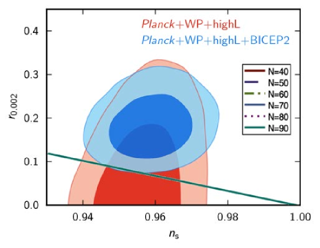
Figure 1: Plots of tensor to scalar ratio (left) and running of scalar spectral index (right) versus scalar spectral index, for a non-minimally kinetic coupled DGP model with $\zeta=10^{-6}$ and the potential $V(\phi)={\sigma}\phi^{\frac{1}{2}}$. The plots are depicted for six values of number of e-folding $N$. For all given viable values of $N$, the non-minimally kinetic coupled DGP model lies inside the $95\%$ CL of the Planck+WP+highL data, but it does not lie in the $95\%$ CL of the Planck+WP+highL+BICEP2 data. The values of running of spectral index are very close to zero for all given values of $N$, and coincides with the prediction of the single monomial chaotic inflationary models with $50<N<60$ (For comparison, there is a purple strip hidden behind the running spectral indexes of non-minimally kinetic coupled DGP model, showing the running spectral index of single monomial chaotic inflationary models with $50<N<60$). The non-minimally kinetic coupled DGP model lies inside the $95\%$ CL of the Planck+WP+BAO:$\Lambda$CDM $dn_{s}/dln_{k}$ data, but it does not lie in the $95\%$ CL of the Planck+WP+BAO:$\Lambda$CDM $dn_{s}/dln_{k}+r$ data.

V.2 $V(\phi)={\sigma}\phi^{\frac{2}{3}}$

The non-minimally kinetic coupled DGP model is well inside the $95\%$ CL of the Planck+WP+highL data, but it does not lie inside the $95\%$ CL of the Planck+WP+highL+BICEP2 data. Evolution of tensor to scalar ratio versus scalar spectral index is shown in the left plot of Fig.2. For all given values of $N$, the non-minimally kinetic coupled DGP model lies inside the $95\%$ CL Planck+WP+highL data. Evolution of the running of scalar spectral index versus scalar spectral index has been plotted in the right panel of Fig.2. For this case, the running is negative and close to zero.

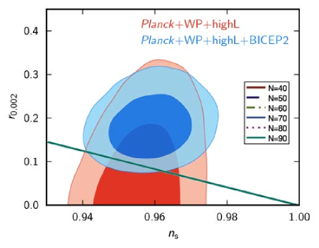
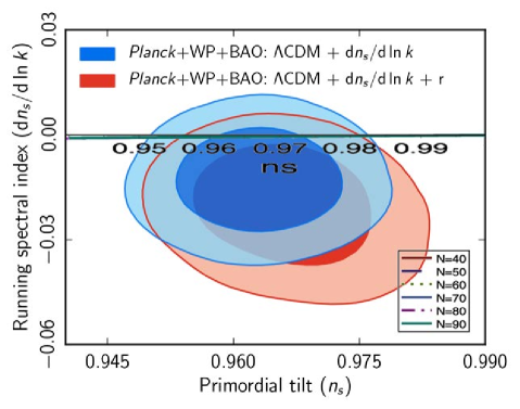
Figure 2: Plots of tensor to scalar ratio (left) and running of scalar spectral index (right) versus scalar spectral index, for a non-minimally kinetic coupled DGP model with $\zeta=10^{-6}$ and $V(\phi)={\sigma}\phi^{{2/3}}$ potential. The figure has been plotted for six values of the number of e-folding. For all given viable values of $N$, the non-minimally kinetic coupled DGP model is well inside the $95\%$ CL Planck+WP+highL data, but it does not lie within the $95\%$ CL Planck+WP+highL+BICEP2 data. The values of running of spectral index are very close to zero for all given values of $N$. The non-minimally kinetic coupled DGP model lies inside the $95\%$ CL of the Planck+WP+BAO:$\Lambda$CDM $dn_{s}/dln_{k}$ data, but it does not lie in the $95\%$ CL of the Planck+WP+BAO:$\Lambda$CDM $dn_{s}/dln_{k}+r$ data.

V.3 $V(\phi)={\sigma}\phi$

A minimally coupled four-dimensional setup with this potential lies within the $95\%$ CL of the Planck+WMAP9+BAO data [26]. Our braneworld model (non-minimally kinetic coupled model), with this linear potential, lies within the $95\%$ CL Planck+WP+highL+BICEP2. A minimally coupled DGP model with this potential lies still inside the $95\%$ CL of the Planck+WMAP9+BAO data. As before, we consider six values of number of e-folding. In the left plot of Fig.3, we see the evolution of tensor to scalar ratio versus scalar spectral index. From our numerical analysis it appears that in a DGP model with non-minimally kinetic coupled gravity, the model lies in the $95\%$ CL Planck+WP+highL+BICEP2, for all given values of $N$. The right plot of Fig.3 shows the evolution of running of scalar spectral index versus scalar spectral index. As the figure shows, for a non-minimally kinetic coupled DGP model with a linear potential, the running of scalar spectral index is close to zero.

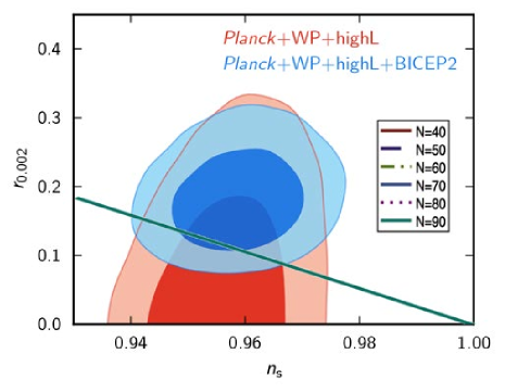
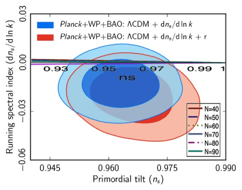
Figure 3: Plots of tensor to scalar ratio (left) and running of scalar spectral index (right) versus scalar spectral index, for a non-minimally kinetic coupled DGP model with $\zeta=10^{-6}$ and a linear potential $V(\phi)\sim\phi$. The figure has been plotted for six values of number of e-folding. For all given viable values of $N$, the non-minimally kinetic coupled DGP model is well inside the $95\%$ CL Planck+WP+highL data and is almost inside the $95\%$ CL Planck+WP+highL+BICEP2 data. The values of running of scalar spectral index are almost zero for all given values of $N$. The non-minimally kinetic coupled DGP model lies inside the $95\%$ CL of the Planck+WP+BAO:$\Lambda$CDM $dn_{s}/dln_{k}$ data, but it does not lie in the $95\%$ CL of the Planck+WP+BAO:$\Lambda$CDM $dn_{s}/dln_{k}+r$ data.

V.4 $V(\phi)={\sigma}\phi^{2}$

In 26 , it has been shown that in 4-dimensions the model with this potential lies outside and inside the $95\%$ CL of the joint Planck+WMAP9+BAO data for $N=50$ and $N=60$, respectively. Now, we explore the situation for a 5-dimensional model. According to the WMAP7+BAO+H₀ data 30 , a warped DGP model with minimally coupled scalar field and with a squared potential, lies inside the $95\%$ CL for $N<70$. Now, with recent BICEP2 date, the situations change considerably. In a minimally coupled DGP model with a quadratic potential, for all $N\geq 40$, the model is outside the joint $95\%$ CL of the Planck+WMAP9+BAO data. In our model for a non-minimally kinetic coupled DGP model, for all given values of $N$ the model is well inside the joint $95\%$ CL Planck+WP+highL+BICEP2 data. The left plot of Fig.4 shows the behavior of tensor to scalar ratio versus scalar spectral index in the background of the Planck+WP+highL+BICEP2 data. This figure has been plotted for six values of $N$. Also, we have plotted the evolution of running of scalar spectral index versus scalar spectral index in the background of the Planck+WP+highL+BICEP2 data (the left panel of Fig.4). We see that, for all six values of the number of e-folding, the running of scalar spectral index is close to zero.

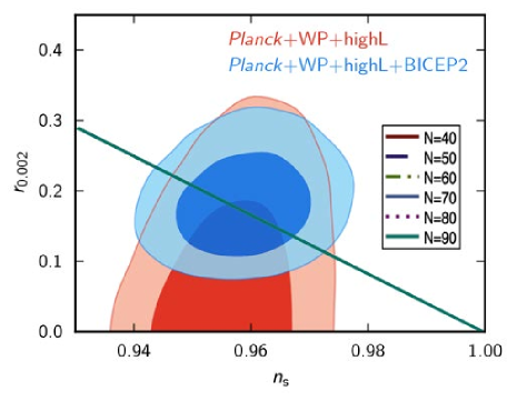
Figure 4: Plots of tensor to scalar ratio (left) and running of scalar spectral index (right) versus scalar spectral index, for a non-minimally kinetic coupled DGP model with $\zeta=10^{-6}$ and a quadratic potential $V(\phi)\sim\phi^{2}$. The figure has been plotted for six values of number of e-folding. For all given viable values of $N$, the non-minimally kinetic coupled DGP model is well inside the $95\%$ CL Planck+WP+highL+BICEP2 data and is almost inside the $95\%$ CL Planck+WP+highL data. The values of the running of spectral index are almost close to zero for all given values of $N$. The non-minimally kinetic coupled DGP model lies almost inside the $95\%$ CL of the Planck+WP+BAO:$\Lambda$CDM $dn_{s}/dln_{k}$ data, but it does not lie in the $95\%$ CL of the Planck+WP+BAO:$\Lambda$CDM $dn_{s}/dln_{k}+r$ data.

V.5 $V(\phi)={\sigma}\phi^{3}$

It has been shown in QingGao that in natural inflation this potential lies in the $95\%$ CL Planck+WP+highL+BICEP2 and also it has been confirmed with WMAP9 31 and Planck 26 data that a model with a cube potentia in 4-dimensions lies outside the $95\%$ CL. In our branworld model, we obtain a different result: a non-minimally kinetic coupled DGP model with this potential, lies inside the $95\%$ CL Planck+WP+highL+BICEP2 data for each given value of $N$. The results are shown in Fig.5. Note that the evolution of running of scalar spectral index corresponding to the cube potential is shown in the right plot of Fig.5. The value of running of scalar spectral index is close to zero.

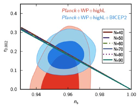
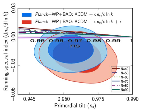
Figure 5: Plots of tensor to scalar ratio (left) and running of scalar spectral index (right) versus scalar spectral index, for a non-minimally kinetic coupled DGP model with $\zeta=10^{-6}$ and a cube potential $V(\phi)\sim\phi^{3}$. The figure has been plotted for $N=40,\,50,\,60,\,70,\,80\,$ and $90$. For all given viable values of $N$ the non-minimally kinetic coupled DGP model is well inside the $95\%$ CL Planck+WP+highL+BICEP2 data and is almost inside the $95\%$ CL Planck+WP+highL data. The values of running of spectral index are approximately zero for all given values of $N$. The non-minimally kinetic coupled DGP model lies approximately close to the $95\%$ CL of the Planck+WP+BAO:$\Lambda$CDM $dn_{s}/dln_{k}$ data, but it does not lie in the $95\%$ CL of the Planck+WP+BAO:$\Lambda$CDM $dn_{s}/dln_{k}+r$ data.

V.6 $V(\phi)=\sigma\phi^{4}$

A minimally coupled 4-dimensional model with this potential lies within the $95\%$ CL of the Planck+WMAP9+BAO data 26 . For $N\leq 70$, our braneworld model (non-minimal kinetic coupled) with this potential lies inside the $95\%$ CL Planck+WP+highL+BICEP2 data. But for all given values of $N$ the model lies inside the $95\%$ CL Planck+WP+highL data. The running of spectral index is plotted in the right plot of Fig.6. In the left plot of Fig.6, we see the evolution of tensor to scalar ratio versus scalar spectral index.

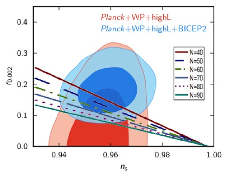
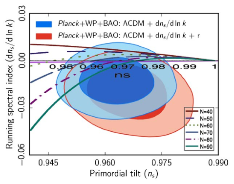
Figure 6: Plots of tensor to scalar ratio (left) and running of scalar spectral index (right) versus scalar spectral index, for a non-minimally kinetic coupled DGP model with $\zeta=10^{-6}$ and a potential of type $V(\phi)\propto\phi^{4}$. The figure has been plotted for $N=40,\,50,\,60\,70,\,80,\,$ and $90$. For all given values of $N$ the model lies inside the $95\%$ CL Planck+WP+highL data and lies inside the $95\%$ CL Planck+WP+highL+BICEP2 data just for $N=40,\,50,\,60,\,70$. The running of spectral index is plotted in the right panel and it is close to zero. Neither of $N=40,\,50,\,60,\,70$ lies inside the $95\%$ CL of the Planck+WP+BAO:$\Lambda$CDM $dn_{s}/dln_{k}$ data and the Planck+WP+BAO:$\Lambda$CDM $dn_{s}/dln_{k}+r$ data.

V.7 $V(\phi)=\sigma\phi^{5}$

Similar to the other cases, we consider six values of the number of e-folding. In the left plot of Fig.7, we see the evolution of tensor to scalar ratio versus scalar spectral index. For all given values of $N$, the non-minimally kinetic coupled DGP braneworld model with this potential lies inside the $95\%$ CL Planck+WP+highL data, but does not lie inside the $95\%$ CL Planck+WP+highL+BICEP2 . The running of spectral index is plotted in the right plot of Fig.7 and it is close to zero.

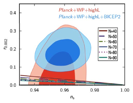
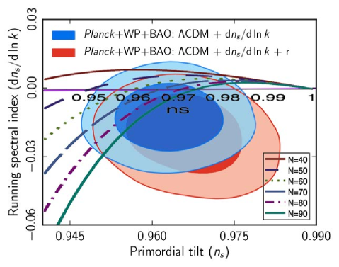
Figure 7: Plots of tensor to scalar ratio (left) and running of scalar spectral index (right) versus scalar spectral index, for a non-minimally kinetic coupled DGP model with $\zeta=10^{-6}$ and a potential of the type $V(\phi)\sim\phi^{5}$. The figure has been plotted for $N=40,\,50,\,60,\,70,\,80,$ and $90$. For all given viable values of $N$, the non-minimally kinetic coupled DGP model lies inside the $95\%$ CL Planck+WP+highL data, but it does not lie inside the $95\%$ CL Planck+WP+highL+BICEP2 data. The running of spectral index is plotted in the right plot of the figure; it is negative for $N\geq 50$, and is positive (close to zero) for $N=40$. The model with values of $N=70,\,80,\,90\,$ and $N=\,80,\,90\,$ lie inside the $95\%$ CL of the Planck+WP+BAO:$\Lambda$CDM $dn_{s}/dln_{k}$ data and the Planck+WP+BAO:$\Lambda$CDM $dn_{s}/dln_{k}+r$ data, respectively.

Our numerical analysis for a DGP model with a non-minimally kinetic coupled provides us with the value of each of the parameters $\phi_{i}$ (the value of $\phi$ at the beginning of inflation), $\phi_{e}$ (the value of $\phi$ at the end of inflation), $H_{i}$ (the value of $H$ at the beginning of inflation), $H_{e}$ (the value of $H$ at the end of inflation), $\varepsilon,\eta$ (the slow-roll parameters), $V(\phi_{i})$ (the value of potential at the beginning of inflation), and $9\zeta H_{i}^{2}{\dot{\phi_{i}}}^{2}$(to control the slow-roll condition $9\zeta H^{2}\dot{\phi}^{2}\ll V(\phi))$ for $N=60$ (the number of e-folding), in the following tables. These values can tell us “which potentials are in best agreement with the recent observations.”

It turns out that the potentials $V(\phi)\propto\phi^{2}$ and $V(\phi)\propto\phi^{3}$ provide respectively the best fits with the observations (see Fig.4, Fig.5 and table.II).

Table 1:

$V(\phi)$	$\sigma$	$\zeta$	$N$	$\phi_{e}$	$H_{e}$	$\phi_{i}$	$H_{i}$	$\varepsilon$	$\eta$	$9fH_{i}^{2}{\dot{\phi_{i}}}^{2}$	$V(\phi_{i})$
${\sigma}\phi^{\frac{1}{2}}$	$1$	$0.001$	$60$	$0.3535$	$0.25705006\sqrt{3}$	$7.76$	$0.5564\sqrt{3}$	$0.0020$	$-0.0062$	$0.007755$	$2.7845$
${\sigma}\phi^{\frac{2}{3}}$	$1$	$0.001$	$60$	$0.4113$	$0.25943584\sqrt{3}$	$8.942$	$0.6919\sqrt{3}$	$0.0027$	$-0.0054$	$0.01856$	$4.308$
${\sigma}\phi$	$1$	$0.001$	$60$	$0.7069$	$0.28030475\sqrt{3}$	$10.977$	$1.1024\sqrt{3}$	$0.0041$	$-0.0040$	$0.11967$	$10.939$
${\sigma}\phi^{2}$	$1$	$0.001$	$60$	$1.4136$	$0.47123562\sqrt{3}$	$14.782$	$4.9273\sqrt{3}$	$0.0075$	$0.000001$	$47.7464$	$218.5075$
${\sigma}\phi^{3}$	$1$	$0.001$	$60$	$0.00008$	$0.00004803\sqrt{3}$	$13.514$	$16.5601\sqrt{3}$	$0.0071$	$0.00098$	$6091.7848$	$2468.1470$
${\sigma}\phi^{4}$	$1$	$0.001$	$60$	$0.0017$	$0.00004805\sqrt{3}$	$11.047$	$40.6787\sqrt{3}$	$0.0041$	$0.0007$	$2.218\times 10^{5}$	$14892.8363$
${\sigma}\phi^{5}$	$1$	$0.001$	$60$	$0.0080$	$0.00004811\sqrt{3}$	$7.902$	$58.5089\sqrt{3}$	$0.0063$	$0.0012$	$9.49\times 10^{6}$	$30809.5338$
${\sigma}\phi^{6}$	$1$	$0.001$	$60$	$0.0203$	$0.00004820\sqrt{3}$	$6.731$	$101.6523\sqrt{3}$	$0.0042$	$0.0094$	$8.46\times 10^{6}$	$92998.8$
${\sigma}e^{\phi}$	$1$	$0.001$	$-$	$"Imaginary"$	$-$	$-$	$-$	$-$	$-$	$-$	$-$

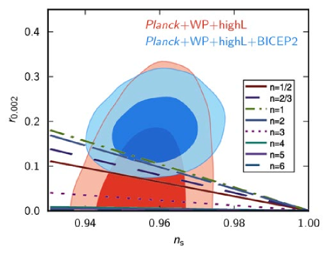
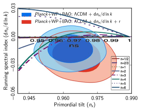
Figure 8: Plots of tensor to scalar ratio (left) and running of scalar spectral index (right) versus scalar spectral index, for a non-minimally kinetic coupled DGP model with $\zeta=10^{-3}$ and a potential of the type $V(\phi)\sim\phi^{n}$. The figure has been plotted for $N=60$. For all given values of $n$, the non-minimally kinetic coupled DGP model lies inside the $95\%$ CL Planck+WP+highL data, but it does not lie inside the $95\%$ CL Planck+WP+highL+BICEP2 data, except $n=1,2$. The running of spectral index is plotted in the right plot of the figure. Neither of the values of $n$ lies inside the $95\%$ CL of the Planck+WP+BAO:$\Lambda$CDM $dn_{s}/dln_{k}+r$ data and all the values of $n$ except $n=5,6$ lie inside the $95\%$ CL of the Planck+WP+BAO:$\Lambda$CDM $dn_{s}/dln_{k}$ data.

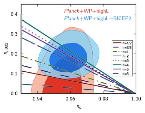
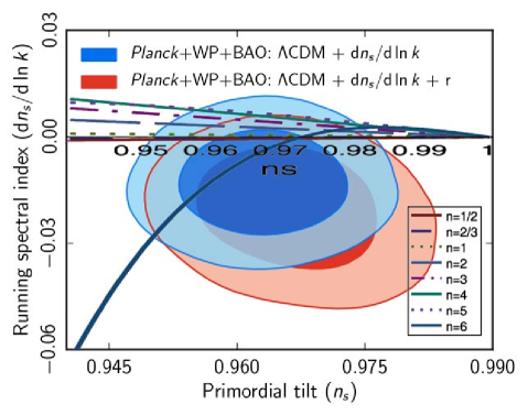
Figure 9: Plots of tensor to scalar ratio (left) and running of scalar spectral index (right) versus scalar spectral index, for a non-minimally kinetic coupled DGP model with $\zeta=10^{-8}$ and a potential of the type $V(\phi)\sim\phi^{n}$. The figure has been plotted for $N=60$. For all given values of $n$, the non-minimally kinetic coupled DGP model lies inside the $95\%$ CL Planck+WP+highL data except $n=3,4$, and lies inside the $95\%$ CL Planck+WP+highL+BICEP2 data, except for $n=1/2,2/3,6$. The running of spectral index is plotted in the right plot of the figure. Neither of the values of $n$ lies inside the $95\%$ CL of the Planck+WP+BAO:$\Lambda$CDM $dn_{s}/dln_{k}+r$ data except $n=6$, and just the values $n=1,2/3,1/2$ lie inside the $95\%$ CL of the Planck+WP+BAO:$\Lambda$CDM $dn_{s}/dln_{k}$ data.

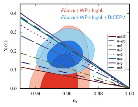
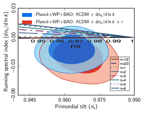
Figure 10: Plots of tensor to scalar ratio (left) and running of scalar spectral index (right) versus scalar spectral index, for a non-minimally kinetic coupled DGP model with $\zeta=10^{-10}$ and a potential of the type $V(\phi)\sim\phi^{n}$. The figure has been plotted for $N=60$. For all given values of $n$, the non-minimally kinetic coupled DGP model lies inside the $95\%$ CL Planck+WP+highL data except $n=3,4,5,6$, and lies inside the $95\%$ CL Planck+WP+highL+BICEP2 data, except $n=1/2,2/3$. The running of spectral index is plotted in the right plot of the figure. Neither of the values of $n$ lies inside the $95\%$ CL of the Planck+WP+BAO:$\Lambda$CDM $dn_{s}/dln_{k}+r$ data, and just the values $n=1,2/3,1/2$ lie inside the $95\%$ CL of the Planck+WP+BAO:$\Lambda$CDM $dn_{s}/dln_{k}$ data.

Table 2:

$V(\phi)$	$\sigma$	$\zeta$	$N$	$\phi_{e}$	$H_{e}$	$\phi_{i}$	$H_{i}$	$\varepsilon$	$\eta$	$9fH_{i}^{2}{\dot{\phi_{i}}}^{2}$	$V(\phi_{i})$
${\sigma}\phi^{\frac{1}{2}}$	$1$	$0.000001$	$60$	$0.3535$	$0.25705006\sqrt{3}$	$7.7540$	$0.5562\sqrt{3}$	$0.0020$	$-0.0062$	$0.000013$	$2.7548$
${\sigma}\phi^{\frac{2}{3}}$	$1$	$0.000001$	$60$	$0.4113$	$0.25943584\sqrt{3}$	$8.9570$	$0.6922\sqrt{3}$	$0.0027$	$-0.0055$	$0.00003$	$4.3130$
${\sigma}\phi$	$1$	$0.000001$	$60$	$0.7070$	$0.28030475\sqrt{3}$	$10.977$	$1.1044\sqrt{3}$	$0.0041$	$-0.0041$	$0.00020$	$10.9770$
${\sigma}\phi^{2}$	$1$	$0.000001$	$60$	$1.4141$	$0.00004803\sqrt{3}$	$15.560$	$5.1867\sqrt{3}$	$0.0082$	$2.5938\times 10^{-8}$	$0.09862$	$242.1146$
${\sigma}\phi^{3}$	$1$	$0.000001$	$60$	$0.00008$	$0.00004803\sqrt{3}$	$18.932$	$27.4583\sqrt{3}$	$0.0124$	$0.0040$	$77.4665$	$6785.6192$
${\sigma}\phi^{4}$	$1$	$0.000001$	$60$	$0.0017$	$0.00004805\sqrt{3}$	$20.850$	$144.9075\sqrt{3}$	$0.0140$	$0.0047$	$60087.2883$	$188983.6520$
${\sigma}\phi^{5}$	$1$	$0.000001$	$60$	$0.0080$	$0.00004811\sqrt{3}$	$17.908$	$452.4043\sqrt{3}$	$0.0095$	$0.0022$	$5.7\times 10^{6}$	$1.84\times 10^{6}$
${\sigma}\phi^{6}$	$1$	$0.000001$	$60$	$0.0203$	$0.00004820\sqrt{3}$	$13.760$	$868.5117\sqrt{3}$	$0.0077$	$0.0018$	$7.7\times 10^{7}$	$6.8\times 10^{6}$
${\sigma}e^{\phi}$	$1$	$0.000001$	$-$	$"Imaginary"$	$-$	$-$	$-$	$-$	$-$	$-$	$-$

Table 3:

$V(\phi)$	$\sigma$	$\zeta$	$N$	$\phi_{e}$	$H_{e}$	$\phi_{i}$	$H_{i}$	$\varepsilon$	$\eta$	$9fH_{i}^{2}{\dot{\phi_{i}}}^{2}$	$V(\phi_{i})$
${\sigma}\phi^{\frac{1}{2}}$	$1$	$10^{-8}$	$60$	$0.3535$	$0.25704370\sqrt{3}$	$7.76$	$0.5564\sqrt{3}$	$0.0020$	$-0.0062$	$7.7\times 10^{-10}$	$2.7856$
${\sigma}\phi^{\frac{2}{3}}$	$1$	$10^{-8}$	$60$	$0.4713$	$0.25943584\sqrt{3}$	$8.962$	$0.6924\sqrt{3}$	$0.0027$	$-0.0055$	$1.86\times 10^{-7}$	$4.3145$
${\sigma}\phi$	$1$	$10^{-8}$	$60$	$0.7070$	$0.28030475\sqrt{3}$	$10.977$	$1.1045\sqrt{3}$	$0.0041$	$-0.0041$	$1.2\times 10^{-6}$	$10.9770$
${\sigma}\phi^{2}$	$1$	$10^{-8}$	$60$	$1.4143$	$0.47146400\sqrt{3}$	$15.562$	$5.1873\sqrt{3}$	$0.0082$	$1.9\times 10^{-8}$	$0.00058$	$242.1758$
${\sigma}\phi^{3}$	$1$	$10^{-8}$	$60$	$0.00008$	$0.00004803\sqrt{3}$	$18.99$	$27.5776\sqrt{3}$	$0.0124$	$0.0041$	$0.4685$	$6844.7143$
${\sigma}\phi^{4}$	$1$	$10^{-8}$	$60$	$0.0017$	$0.00004805\sqrt{3}$	$21.91$	$160.016\sqrt{3}$	$0.0166$	$0.0082$	$531.0547$	$230446.1$
${\sigma}\phi^{5}$	$1$	$10^{-8}$	$60$	$0.0080$	$0.00004811\sqrt{3}$	$17.908$	$962.8047\sqrt{3}$	$0.0197$	$0.0244$	$6.960\times 10^{5}$	$8.343\times 10^{6}$
${\sigma}\phi^{6}$	$1$	$10^{-8}$	$60$	$0.0203$	$0.00004820\sqrt{3}$	$25.437$	$5486.2\sqrt{3}$	$0.0075$	$0.0020$	$7.33\times 10^{8}$	$2.7\times 10^{8}$
${\sigma}e^{\phi}$	$1$	$10^{-8}$	$-$	$"Imaginary"$	$-$	$-$	$-$	$-$	$-$	$-$	$-$

Table 4:

$V(\phi)$	$\sigma$	$\zeta$	$N$	$\phi_{e}$	$H_{e}$	$\phi_{i}$	$H_{i}$	$\varepsilon$	$\eta$	$9fH_{i}^{2}{\dot{\phi_{i}}}^{2}$	$V(\phi_{i})$
${\sigma}\phi^{\frac{1}{2}}$	$1$	$10^{-10}$	$60$	$0.3535$	$0.25705007\sqrt{3}$	$7.7540$	$0.5562\sqrt{3}$	$0.0020$	$-0.0062$	$7.7\times 10^{-10}$	$2.7845$
${\sigma}\phi^{\frac{2}{3}}$	$1$	$10^{-10}$	$60$	$0.4713$	$0.25943584\sqrt{3}$	$8.962$	$0.6924\sqrt{3}$	$0.0027$	$-0.0055$	$1.86\times 10^{-9}$	$4.3145$
${\sigma}\phi$	$1$	$10^{-10}$	$60$	$0.7070$	$0.28030475\sqrt{3}$	$10.977$	$1.1045\sqrt{3}$	$0.0041$	$-0.0041$	$1.2\times 10^{-8}$	$10.9770$
${\sigma}\phi^{2}$	$1$	$10^{-10}$	$60$	$1.4141$	$0.471392\sqrt{3}$	$15.560$	$5.1867\sqrt{3}$	$0.0082$	$2.5\times 10^{-8}$	$5.8\times 10^{-6}$	$242.1745$
${\sigma}\phi^{3}$	$1$	$10^{-10}$	$60$	$0.00008$	$0.00004803\sqrt{3}$	$18.99$	$27.5776\sqrt{3}$	$0.0124$	$0.0041$	$0.0047$	$6844.7143$
${\sigma}\phi^{4}$	$1$	$10^{-10}$	$60$	$0.0017$	$0.00004805\sqrt{3}$	$21.91$	$160.0165\sqrt{3}$	$0.0140$	$0.0107$	$5.3105$	$230446.1$
${\sigma}\phi^{5}$	$1$	$10^{-10}$	$60$	$0.0080$	$0.00004811\sqrt{3}$	$17.908$	$989.8567\sqrt{3}$	$0.0208$	$0.0022$	$7776.326$	$8.818\times 10^{6}$
${\sigma}\phi^{6}$	$1$	$10^{-10}$	$60$	$0.0203$	$0.00004820\sqrt{3}$	$26.72$	$6358.9895\sqrt{3}$	$0.02043$	$0.0152$	$1.324\times 10^{7}$	$3.639\times 10^{8}$
${\sigma}e^{\phi}$	$1$	$10^{-10}$	$-$	$"Imaginary"$	$-$	$-$	$-$	$-$	$-$	$-$	$-$

VI conclusion and remarks

In this paper, we have considered a $5D$ bulk spacetime together with a single $4D$ brane and derived the effective $4D$ gravitational equations. Then, we have studied the non-minimally kinetic coupled version of a braneworld gravity proposed by Dvali, Gabadadze, and Porrati, so called DGP model. We have derived the field equations, using the FRW metric accompanied by the perfect fluid, and studied the inflationary scenario in this model. Finally, we have confronted the numerical analysis of six typical scalar field potentials with the observational data, and found that:

• For $V(\phi)=\sigma\phi^{\frac{1}{2}}$ and $V(\phi)=\sigma\phi^{\frac{2}{3}}$ and the given values of $N$, the non-minimally kinetic coupled DGP model is well inside the $95\%$ CL of the Planck+WP+highL data, but does not lie in the $95\%$ CL of the Planck+WP+highL+BICEP2. So, these potentials cannot provide the best fits with the current observations (see Fig.1 and Fig.2).

• For $V(\phi)=\sigma\phi$ and the given values of $N$, the non-minimally kinetic coupled DGP model is well inside the $95\%$ CL Planck+WP+highL+BICEP2 data. But, the evolution of tensor to scalar ratio versus scalar spectral index cannot provide the best fits with the current observations (see Fig.3).

• For $V(\phi)=\sigma\phi^{2}$ and the given values of $N$, the non-minimally kinetic coupled DGP model is well inside the $95\%$ CL Planck+WP+highL+BICEP2 data and the evolution of tensor to scalar ratio versus scalar spectral index provides the best fits with the current observations (see Fig.4).

• For $V(\phi)=\sigma\phi^{3}$ and the given values of $N$, the non-minimally kinetic coupled DGP model is well inside the $95\%$ CL Planck+WP+highL+BICEP2 data and the evolution of tensor to scalar ratio versus scalar spectral index provides the best fits with the current observations (see Fig.5).

• For $V(\phi)=\sigma\phi^{4}$ and $N\leq 60$, the non-minimally kinetic coupled DGP model is well inside the $95\%$ CL Planck+WP+highL+BICEP2 data. Since the number of e-folding should be usually lager than 60 and because this potential cannot satisfy the slow-roll condition (i.e. $9\zeta H^{2}\dot{\phi}^{2}\ll V(\phi)$), it is not a good potential for inflation in this model (see Table II).

• For $V(\phi)=\sigma\phi^{5}$ and the potentials with powers more than 5, one can show that for the given values of $N$ the non-minimally kinetic coupled DGP model is well inside the $95\%$ CL of the Planck+WP+highL data, but does not lie in the $95\%$ CL of the Planck+WP+highL+BICEP2. Moreover, these potentials cannot satisfy the slow-roll condition (i.e $9\zeta H^{2}\dot{\phi}^{2}\ll V(\phi)$), hence cannot be considered as good potentials for inflation in this model (see Fig7 and Table II).

• For $V(\phi)=\sigma\ln(\phi)$ and $V(\phi)=\sigma e^{\pm\phi}$ and the given values of $N$, we get the imaginary value of $\phi$ at the end of inflation (i.e. $\phi_{e}$). So, these potentials cannot be considered as good potentials for inflation in this model (see Table II).

• For given scalar field potentials with $n=1/2,2/3,1,2,3,4,5,6$, $N=60$ and $\zeta=10^{-3}$ the non-minimally kinetic coupled DGP model lies inside the $95\%$ CL Planck+WP+highL data, and lies inside the $95\%$ CL Planck+WP+highL+BICEP2 data, for $n=1,2$ (see Fig.8 and table I).

• For given scalar field potentials with $n=1/2,2/3,1,2,3,4,5,6$, $N=60$ and $\zeta=10^{-8}$, the non-minimally kinetic coupled DGP model lies inside the $95\%$ CL Planck+WP+highL data for $n=1/2,2/3,1,2$, and lies inside the $95\%$ CL Planck+WP+highL+BICEP2 data, for $n=1,2,3,4,5,6$ (see Fig.9 and table III).

• For given scalar field potentials with $n=1/2,2/3,1,2,3,4,5,6$, $N=60$ and $\zeta=10^{-10}$, the non-minimally kinetic coupled DGP model lies inside the $95\%$ CL Planck+WP+highL data for $n=1/2,2/3,1,2$, and lies inside the $95\%$ CL Planck+WP+highL+BICEP2 data, for $n=1,2,3,4,5,6$ (see Fig.10 and table IV).

In conclusion, in the study of inflation using the non-minimally kinetic coupled DGP model, we found that among the suggested potentials and coupling constants, subject to the e-folding $N=60$ required by inflationary scenario, the potentials $V(\phi)=\sigma\phi$, $V(\phi)=\sigma\phi^{2}$ and $V(\phi)=\sigma\phi^{3}$ provide the best fits with both Planck+WP+highL data and Planck+WP+highL+BICEP2 data.