Equilibria, Dynamics and Current Sheets Formation
in magnetically confined coronae

Abstract

The dynamics of magnetic fields in closed regions of solar and stellar coronae are investigated with a reduced magnetohydrodynamic (MHD) model in the framework of Parker scenario for coronal heating. A novel analysis of reduced MHD equilibria shows that their magnetic fields have an asymmetric structure in the axial direction with variation length-scale $z_{\ell}\sim\ell B_{0}/b$, where $B_{0}$ is the intensity of the strong axial guide field, $b$ that of the orthogonal magnetic field component, and $\ell$ the scale of $\mathbf{b}$. Equilibria are then quasi-invariant along the axial direction for variation scales larger than approximatively the loop length $z_{\ell}\gtrsim L_{z}$, and increasingly more asymmetric for smaller variation scales $z_{\ell}\lesssim L_{z}$. The critical length $z_{\ell}\sim L_{z}$ corresponds to the magnetic field intensity threshold $b\sim\ell B_{0}/L_{z}$. Magnetic fields stressed by photospheric motions cannot develop strong axial asymmetries. Therefore fields with intensities below such threshold evolve quasi-statically, readjusting to a nearby equilibrium, without developing nonlinear dynamics nor dissipating energy. But stronger fields cannot access their corresponding asymmetric equilibria, hence they are out-of-equilibrium and develop nonlinear dynamics. The subsequent formation of current sheets and energy dissipation is necessary for the magnetic field to relax to equilibrium, since dynamically accessible equilibria have variation scales larger than the loop length $z_{\ell}\gtrsim L_{z}$, with intensities smaller than the threshold $b\lesssim\ell B_{0}/L_{z}$. The dynamical implications for magnetic fields of interest to solar and stellar coronae are investigated numerically and the impact on coronal physics discussed.

1. Introduction

Solar observations show a close association between magnetic field strength and coronal activity. In combination with the ability of photospheric motions to stress the field, these are the two key elements to understand the observed coronal X-ray activity of the Sun, of all late-type main sequence stars, and more in general of stars with a magnetized corona and an outer convective envelope (Güdel, 2004, 2009).

It has long been proposed that the work done by photospheric motions on magnetic field line footpoints can transform mechanical energy into magnetic energy and transfer it in the upper corona. The photospheric (horizontal) velocity can be split into irrotational and solenoidal components. Only its solenoidal (incompressible) component has a non-vanishing vorticity and can then twist the magnetic field lines, injecting magnetic energy into the corona.

Gold & Hoyle (1960) conjectured that the magnetic field would proceed through a sequence of force-free equilibria while photospheric vortices twist the field lines, and the stored energy could subsequently be released when two flux tubes with similarly twisted field lines come into contact with each other, or when the configuration would become somehow unstable through an undetermined mechanism (Gold, 1964). Sturrock & Uchida (1981) compute the energy flux into the corona due to the work done by random photospheric vortical motions on the magnetic field. They find that the correlation time of photospheric motions must be of the order of the observed photospheric timescales (5-8 minutes) or longer to obtain an energy flux large enough to sustain an active corona, otherwise for shorter correlation times the resulting twisted field is too small. But the magnetic energy is still supposed to be stored in a force-free field in equilibrium, and no physical mechanism able to dissipate this energy and heat the corona is envisioned.

Energy stored in a magnetic field in equilibrium, that subsequently becomes unstable and releases its energy, is the common thread of flare models (Shibata & Magara, 2011; Martin et al., 2012), with the processes leading to the pre-flare magnetic energy storage and its subsequent fast release strongly debated. On the other hand this picture does not appear apt to describe the dynamics of the long-lived slender X-ray bright loops, that in comparison to a flare show little dynamics from their large-scales down to the smallest resolved scale ($\sim 150$ km) of current state-of-the-art X-ray and EUV imagers on board Hinode, SDO and Hi-C (Peter et al., 2013). While the pre-flare magnetic structure is destroyed during the flare, the large-scale magnetic topology of the loops where the basic heating occurs, and that make the corona shine steadily in X-ray, is not strongly modified on comparable timescales. This suggests that the energy deposition must occur at very small scales yet observationally unresolved. Furthermore the energy reservoir that supplies dissipation should consist of magnetic field fluctuations (with vanishing time-average, but non vanishing time-averaged rms) that adds up to the strong axial magnetic field that defines the loop.

Parker (1972, 1988, 1994, 2012) was the first to suggest that, in contrast to previous quasi-static models, the magnetic field brought about by photospheric vortical motions would be in dynamical non-equilibrium in the case of interest to coronal heating. Furthermore the relaxation of this interlaced fields toward equilibrium would necessarily involve the formation of current sheets. The energy dissipation would then occur at small scales in the fashion of small impulsive heating events, so-called nanoflares, a picture broadly used for the thermodynamical modeling of the closed corona (Klimchuk, 2006; Reale, 2014).

Using a simplified Cartesian model with a strong guide field threading a coronal loop, Parker (1972, 1979) argued at first that a magnetic field could be in equilibrium only if it were invariant along $z$ (the axial direction). Due to the complex and disordered nature of photospheric motions the induced interlaced magnetic field would not be invariant, and therefore not in equilibrium. Next, counterexamples of magnetostatic equilibria that are not invariant along $z$ were provided (Rosner & Knobloch, 1982; Bogoyavlenskij, 2000), and analytical investigations (van Ballegooijen, 1985; Antiochos, 1987; Cowley et al., 1997) argued that smooth photospheric motions cannot lead to the formation of current sheets, whereas only a discontinuous velocity field can form discontinuities in the coronal magnetic field.

In particular van Ballegooijen (1985) showed that the equilibria are the solutions of the two-dimensional (2D) Euler equation that in general are not $z$-invariant, thus inferring that the field would evolve quasi-statically, continuously readjusting to a nearby force-free equilibrium without developing nonlinear dynamics nor forming current sheets. Reaching opposite conclusions Parker (1988, 1994, 2000, 2012) pointed out that almost all field line topologies relevant to the solar corona have a different structure from the solutions of the Euler equation, so that the magnetic field would be still in dynamical non-equilibrium.

Reduced magnetohydrodynamics (MHD) numerical simulations with a continuous smooth velocity forcing at the boundaries show that the dynamics can be seen as a particular instance of magnetically dominated MHD turbulence (Dmitruk & Gómez, 1999; Dmitruk et al., 2003; Rappazzo et al., 2007, 2008) as proposed by earlier 2D models (Einaudi et al., 1996; Dmitruk & Gómez, 1997), suggesting that in the forced case the magnetic field is in dynamical non-equilibrium rather than close to a quasi-static evolution. Similar dynamics are also displayed by boundary driven simulations in the cold plasma regime (Hendrix & van Hoven, 1996) and in the fully compressible MHD case (Galsgaard & Nordlund, 1996; Dahlburg et al., 2012). Furthermore Rappazzo & Velli (2011) have shown that while velocity fluctuations are much smaller than magnetic fluctuations, spectral energy fluxes toward smaller scales are akin to those of a standard cascade with magnetic and kinetic energies in equipartition, except for kinetic energy fluxes that are negligible. This implies that at scales smaller than those directly shuffled by photospheric motions, the small velocity field is created and shaped by the unbalanced Lorentz force of the out-of-equilibrium magnetic field, that in turn creates small scales in the magnetic field by distorting magnetic islands and pushing field lines together. Additionally Georgoulis et al. (1998); Dmitruk et al. (1998) have established a link between boundary driven simulations and observed statistics of coronal activity. Indeed the bursts in dissipation displayed by the system, that correspond to the formation and dissipation of current sheets, follow a power law behavior in total energy, peak dissipation and duration with indexes not far from those determined observationally in X-rays.

Recently Wilmot-Smith et al. (2009) have shown that the relaxation of a slightly braided magnetic field (“pigtail” braid) appears to evolve quasi-statically, with no formation of current sheets, toward an equilibrium where only large-scale current layers of thickness much larger than the resolution scale are observed. This result would seem in contrast with Parker’s hypothesis, the results of the forced numerical simulations discussed in the previous paragraph, and the recent results supporting the development of finite time singularities in the cold plasma regime (Low, 2013, 2015).

To get further insight on the dynamics of coronal magnetic fields, Rappazzo & Parker (2013) analyzed reduced MHD numerical simulations of the relaxation of initial magnetic fields invariant along $z$ and with different average twists. They identified a critical intensity threshold for the magnetic field. This is explained heuristically as due to a balance between different field line tension forces for weak fields, while such a balance cannot be attained by stronger fields. The non-equilibrium of stronger fields stems from this force unbalance, and drives the relaxation forming current sheets and dissipating energy. On the contrary weaker fields show little dynamics with no energy dissipation, confirming that they are essentially in equilibrium. Such threshold can explain qualitatively the result of Wilmot-Smith et al. (2009), although a quantitative comparison cannot be made because the integrated equations (magneto-frictional relaxation vs. reduced MHD) and initial topologies differ.

The magnetic intensity threshold found by Rappazzo & Parker (2013) implies that a critical twist exists above which dynamics develop, and below which the system remains very close to equilibrium. Parker (1988) had conjectured that a critical twist is necessary to explain the observationally inferred energy flux in active regions (Withbroe & Noyes, 1977). In fact the energy flux injected in the corona by photospheric motions is the average Poynting flux $\langle S_{z}\rangle=B_{0}\,\langle\mathbf{u}_{\textrm{ph}}\cdot\mathbf{b}\rangle$ (see Section 2.2, Equation [7]) that depends not only on the photospheric velocity $\mathbf{u}_{\textrm{ph}}$ and the axial guide field $B_{0}$, but also on the dynamic magnetic field component $\mathbf{b}$, with stronger intensities corresponding to higher average twists. Thus if nonlinear dynamics were to develop for weak field intensities, energy dissipation would keep too low the value of $\mathbf{b}$, and consequently the flux $\langle S_{z}\rangle$. This argument is further reinforced by the fact that current sheets thickness decreases at least exponentially in time when nonlinear dynamics develop, reaching the Sweet-Parker thickness (Sweet, 1958; Parker, 1957) on ideal timescales (about one Alfvén crossing time $\tau_{A}$, Rappazzo & Parker, 2013), that current sheets are unstable to tearing modes with “ideal” growth rates (i.e., of order 1/$\tau_{A}$) already at thicknesses larger than Sweet-Parker (Pucci & Velli, 2014; Tenerani et al., 2015; Landi et al., 2015), and that magnetic reconnection rates can be very fast in plasmas with high Reynolds numbers (Lazarian & Vishniac, 1999; Loureiro et al., 2007; Lapenta, 2008; Loureiro et al., 2009; Uzdensky et al., 2010; Huang & Bhattacharjee, 2010; Beresnyak, 2013) and in the collisionless regime (Shay et al., 1999; Birn et al., 2001).

This paper is devoted to a more detailed discussion and analysis of the numerical simulations described by Rappazzo & Parker (2013), of additional simulations that extend our previous work to initial conditions non-invariant along $z$, and to a novel analysis of the structure of the reduced MHD equilibria, with the goal to shed light on the topics outlined in this introduction and advance our understanding of coronal magnetic field dynamics, their relationship to dynamic non-equilibrium, MHD turbulence, quasi-static evolution, current sheets formation and activity of solar and stellar coronae.

The loop model along with initial and boundary conditions for the simulations are introduced in Section 2. The structure of the equilibria is analyzed in Section 3, and the results of the numerical simulations are described in Section 4. Finally results and conclusions are summarized in Section 5, together with a discussion of their impact on coronal physics.

2. Physical Model

A closed region of the solar corona is modeled, as in previous work (Rappazzo et al., 2007), with a simplified cartesian geometry, uniform density $\rho$ and a strong and homogeneous axial magnetic field $\mathbf{B}_{0}=B_{0}\,\mathbf{\hat{e}}_{z}$ threading the system. Plasmas in such configurations are well suited to be studied in the reduced MHD regime (Zank & Matthaeus, 1992). Introducing the velocity and magnetic field potentials $\varphi$ and $\psi$, for which $\mathbf{u}=\nabla\varphi\times\mathbf{\hat{e}}_{z}$, $\mathbf{b}=\nabla\psi\times\mathbf{\hat{e}}_{z}$, vorticity $\omega=-\nabla^{2}_{\!{}_{\!\perp}}\varphi$, and the current density $j=-\nabla^{2}_{\!{}_{\!\perp}}\psi$, the nondimensional reduced MHD equations (Kadomtsev & Pogutse, 1974; Strauss, 1976) are:

$$\partial_{t}\psi=\left[\varphi,\psi\right]+B_{0}\,\partial_{z}\varphi+\eta_{{}_{n}}\nabla_{{}_{\!\!\perp}}^{2n}\psi,\quad$$ (1)

$$\partial_{t}\omega=\left[j,\psi\right]-\left[\omega,\varphi\right]+B_{0}\,\partial_{z}j+\nu_{{}_{\!n}}\nabla_{{}_{\!\!\perp}}^{2n}\omega.$$ (2)

The Poisson bracket of functions $g$ and $h$ is defined as $[g,h]=\partial_{x}g\,\partial_{y}h-\partial_{y}g\,\partial_{x}h$ (e.g., $[j,\psi]=\mathbf{b}\cdot\nabla j$), and Laplacian operators have only orthogonal components. To render the equations nondimensional the magnetic fields are first expressed as Alfvén velocities ($b\rightarrow b/\sqrt{4\pi\rho}$), and then all velocities are normalized with $u^{\ast}=1$ km s^-1, a typical value for photospheric motions. The domain spans $0\leq x,y\leq L_{\perp}$ and $0\leq z\leq L_{z}$, with $L_{\perp}=1$ and $L_{z}=10$. Magnetic field lines are line-tied to a motionless photosphere at the top and bottom plates ($z=0$ and $10$), where a vanishing velocity $\mathbf{u}=0$ is in place. In the perpendicular ($x$-$y$) directions a pseudo-spectral scheme with periodic boundary conditions and isotropic truncation de-aliasing is used ($2/3$-rule, Canuto et al., 2006), while along $z$ a second-order finite difference scheme is implemented. The CFL (Courant-Friedrichs-Levy) condition is satisfied through an adaptive time-step. For a more detailed description of the model and numerical code see Rappazzo et al. (2007, 2008).

Dissipative simulations use hyper-diffusion (Biskamp, 2003), that effectively limits diffusion to the small scales, with $n=4$ and $\nu_{n}=\eta_{n}=\left(-1\right)^{n+1}/R_{n}$, with $R_{n}$ corresponding to the Reynolds number for $n=1$ (see Rappazzo et al., 2008).

2.1. Initial and boundary conditions

Simulations are started at time $t=0$ with a vanishing velocity $\mathbf{u}=0$ everywhere, and a uniform and homogeneous guide field $B_{0}$. The orthogonal field $\mathbf{b}$ consists of large-scale Fourier modes, set expanding the magnetic potential in the following way:

$$\psi_{0}=b_{0}\sum_{rsm}(2\mathscr{E}_{{}_{m}})^{\frac{1}{2}}\ \frac{\alpha_{rsm}\ \sin\left(\mathbf{k}_{rsm}\!\cdot\mathbf{x}+2\pi\xi_{rsm}\right)}{k_{rs}\ \sqrt{\sum_{ij}\alpha^{2}_{ijm}}}$$ (3)

$$\textrm{with}\quad\mathbf{k}_{rsm}=\frac{2\pi}{L_{\perp}}\left(r\,\mathbf{\hat{e}}_{x}+s\,\mathbf{\hat{e}}_{y}\right)+\frac{2\pi}{L_{z}}m\,\mathbf{\hat{e}}_{z},$$

$$\textrm{and}\quad k_{rs}=\frac{2\pi}{L_{\perp}}\sqrt{r^{2}+s^{2}},$$

where the coefficients $\alpha_{rsm}$ and $\xi_{rsm}$ are two independent sets of random numbers uniformly distributed between 0 and 1. The orthogonal wave-numbers $(r,s)$ are always in the range $3\leq(r^{2}+s^{2})^{1/2}\leq 4$, while the parallel amplitudes $\mathscr{E}_{m}$ (with $\sum_{m}\mathscr{E}_{m}=1$) are set to distribute the energy in different ways in the axial direction. Given the orthogonality of the base used in Eq. (3) the normalization factors guarantee that for any choice of the amplitudes the rms of the magnetic field is set to $b=\langle b_{x}^{2}+b_{y}^{2}\rangle^{1/2}=b_{0}$, while for total magnetic energy $E_{{}_{\!M}}=b_{0}^{2}V/2\sum_{m}\mathscr{E}_{m}$, i.e., $\mathscr{E}_{m}$ is the fraction of magnetic energy in the parallel mode $m$. Two-dimensional (2D) configurations invariants along $z$ are obtained considering the single mode $m=0$ with $\mathscr{E}_{0}=1$.

2.2. Energetics

From equations (1)-(2), with $n=1$ and considering the kinetic and magnetic Reynolds numbers equal, the following energy equation can be obtained:

$$\frac{\partial}{\partial t}\ \frac{1}{2}\left(\mathbf{u}^{2}+\mathbf{b}^{2}\right)=-\nabla\cdot\left(\mathbf{S}+\mathbf{F}\right)-\frac{1}{R}\left(j^{2}+\omega^{2}\right),$$ (4)

where $\mathbf{S}=\mathbf{B}\times(\mathbf{u}\times\mathbf{B})$ is the Poynting vector, and $\mathbf{F}=(p+\mathbf{u}^{2}/2)\mathbf{u}-(\omega\mathbf{u}+j\mathbf{b})\times\mathbf{\hat{e}}_{z}/R$ is an orthogonal transport-related flux. Integrating equation (4) over the whole box the energy ($E$) equation is

$$\frac{\partial E}{\partial t}=S-\frac{1}{R}\int_{V}\mathrm{d}V\left(j^{2}+\omega^{2}\right),$$ (5)

i.e., as expected, the global energy balance depends on the competition between the energy flowing into the computational box from the photospheric boundaries $S$ and the ohmic and viscous dissipation. Because in the x–y planes periodic boundary conditions are implemented, and $F_{z}=0$, the only relevant component of the flux vectors is that of the Poynting vector along the axial direction $S_{z}$ that, as $\mathbf{B}=B_{0}\mathbf{\hat{e}}_{z}+\mathbf{b}$, is given by

$$S_{z}=\mathbf{S}\cdot\mathbf{\hat{e}}_{z}=-B_{0}\left(\mathbf{u}\cdot\mathbf{b}\right).$$ (6)

Indicating the photospheric velocity fields at the top and bottom boundaries $z=0$ and $L$ with $\mathbf{u}^{0}$ and $\mathbf{u}^{L}$ for the integrated energy flux (i.e., the power) $S$ we obtain

$$S=B_{0}\int\limits_{z=L}\mathrm{d}a\left(\mathbf{u}^{L}\cdot\mathbf{b}\right)-B_{0}\int\limits_{z=0}\mathrm{d}a\left(\mathbf{u}^{0}\cdot\mathbf{b}\right).$$ (7)

The injected energy power is proportional to $B_{0}$ and depends on the dot product of the photospheric velocities $\mathbf{u}^{0,L}$ and the magnetic field $\mathbf{b}$ at the boundaries. But while $\mathbf{u}^{0,L}$ and $B_{0}$ have fixed values (in our simplified model), the magnetic field $\mathbf{b}$ is determined by the linear or nonlinear dynamics developing in the computational box.

Since the magnetic field component $\mathbf{b}$ can often be considered quasi-invariant along $z$ (as described in the following sections), as a shorthand we will indicate the difference between the boundary velocities with $\mathbf{u}_{ph}=\mathbf{u}^{L}-\mathbf{u}^{0}$, so that for quasi-invariant fields the Poynting flux can be approximated as $\langle S_{z}\rangle\sim S/\ell^{2}\sim B_{0}u_{ph}b$.

3. Equilibria and their dynamic accessibility: Analysis

As discussed in the introduction, the properties of the equilibria of this system are pivotal to understand its dynamics (Parker, 1972, 1988, 1994; van Ballegooijen, 1985, 1986), therefore their structure is analyzed here in detail. It is shown that, depending on the ratio $b_{0}/B_{0}$ of the rms of the orthogonal component to the guide magnetic field intensity, the equilibria can be approximately invariant along $z$ or strongly asymmetric. As shown in the following this can explain why fields with a twist below a critical value do not form strong current sheets, while they do at higher twists as conjectured by Parker (1988). Nevertheless unlike commonly thought, such equilibria are generally not linearly unstable for most conditions relevant to coronal loops, since they arise from a balance of forces in an asymmetric and irregular topology.

Neglecting velocity and diffusion terms, equilibria of Eqs. (1)-(2) are given by $\mathbf{B}\cdot\nabla j=0$. Since the total magnetic field $\mathbf{B}$ is given by $\mathbf{B}=B_{0}\mathbf{\hat{e}}_{z}+\mathbf{b}(x,y,z)$ with $\mathbf{b}\cdot\mathbf{\hat{e}}_{z}=0$, the equilibrium condition can be written as:

$$\frac{\partial j}{\partial z}=-\frac{\mathbf{b}}{B_{0}}\cdot\nabla j,$$ (8)

where the right-hand side term corresponds to the “2D perpendicular” Lorentz force component $\mathbf{b}\cdot\nabla\mathbf{b}$, and the left hand side to the “parallel” $B_{0}\partial_{z}\mathbf{b}$ field line tension (the labels refer to their derivative, but both components are orthogonal to $B_{0}$, a more detailed discussion is in Section 4.1 prior to Equation [23]).

Assigned $\mathbf{b}$ in an x-y plane, e.g., at the boundary z=0 $\mathbf{b}(x,y,z=0)=\mathbf{b}_{bd}(x,y)$, the integration of this equation for $z>0$ allows to compute the corresponding equilibrium in the whole computational box $0\leq z\leq L_{z}$.

Now consider the 2D Euler equation (Euler, 1761)

$$\frac{\partial\omega}{\partial t}=-\mathbf{u}\cdot\nabla\omega,$$ (9)

with $\nabla\cdot\mathbf{u}=0$. Introducing the velocity potential $\phi$, then $\mathbf{u}(x,y,t)=\nabla\phi(x,y,t)\times\mathbf{\hat{e}}_{z}$, and vorticity $\omega=-\nabla^{2}\phi$. The two equations (8) and (9) are identical under the mapping

$$\left\{\begin{aligned} &\\[-10.00002pt] &t\rightarrow z,\\[1.00006pt] &\mathbf{u}\rightarrow\frac{\mathbf{b}}{B_{0}},\\[-13.00005pt] &\end{aligned}\right.$$ (10)

and consequently $\omega\rightarrow j/B_{0}$.

The related 2D Navier-Stokes equation is obtained by adding to the right hand side of Equation (9) the dissipative term $\nu\nabla^{2}\omega$, from which the 2D Euler equation is recovered for $\nu=0$. The physics and solutions of the 2D Euler and Navier-Stokes equations have been studied extensively theoretically, numerically and in the laboratory, in the framework of 2D hydrodynamic turbulence (see reviews by Kraichnan & Montgomery, 1980; Tabeling, 2002; Boffetta & Ecke, 2012). Unlike the 3D case, it has been shown that given a smooth initial condition $\mathbf{u}_{0}(x,y)$ at time $t=0$ the 2D Euler equation admits a unique and regular solution at $t>0$, i.e., no finite time singularity develops (Rose & Sulem, 1978; Chemin, 1993; Bertozzi & Constantin, 1993; Majda & Bertozzi, 2001).

In 2D in addition to energy, also mean-square vorticity (enstrophy) is conserved. The coupled conservation constraints have a strong impact on the dynamics that differs considerably from its 3D hydrodynamic counterpart and the corresponding magnetohydrodynamic cases. In particular, indicating the Energy with $E=(1/2)\langle\mathbf{u}^{2}\rangle$ (the integrated square velocity), the enstrophy with $\Omega=(1/2)\langle\omega^{2}\rangle$, and the palinstrophy with $P=(1/2)\langle|\nabla\omega|^{2}\rangle$, the following energy and enstrophy conservation equations are obtained from the 2D Navier-Stokes equations (e.g., Boffetta & Ecke, 2012):

$$\frac{dE}{dt}=-2\nu\Omega=-\epsilon_{\nu}(t),\qquad\frac{d\Omega}{dt}=-2\nu P.$$ (11)

Since all quantities ($E$, $\Omega$, $P$, and $\nu$) are positively defined, it follows that $\Omega$ can at most decrease. Therefore the energy dissipation rate $\epsilon_{\nu}$ vanishes as viscosity tends to zero:

$$\lim_{\nu\to 0}\epsilon_{\nu}=0.$$ (12)

This result strongly differs from the 3D case where, in the K41 phenomenology introduced by Kolmogorov (1941), for a sufficiently small viscosity the energy dissipation rate is approximately constant $\epsilon_{\nu}\sim\textrm{const}$ and independent from viscosity. This dissipative anomaly in 3D was first pointed out by Taylor (1935), and later confirmed in laboratory experiments (Dryden, 1943; Sreenivasan, 1984; Pearson et al., 2002) and by hydrodynamic numerical simulations (Sreenivasan, 1998; Kaneda et al., 2003).

Thus, in contrast to the 3D case, Equation (12) implies that for small viscosities 2D turbulence is essentially unable to dissipate energy at small scales. The viscous sink of energy is missing, because at any given time during the decay of an initial large-scale velocity field, for a sufficiently small value of $\nu$, the dissipation is arbitrarily small.

Therefore in two dimensions there cannot be a direct energy cascade. As proposed by Kraichnan (1967), energy must flow toward the larger scales through an inverse cascade. Thus during their evolution vortices (velocity eddies) acquire increasingly larger scales, while it is enstrophy that develops a direct cascade (Batchelor, 1969) with vorticity acquiring smaller scales. As can be seen from Equation (9) the convective derivative of $\omega$ vanishes as $\nu$ tends to zero, i.e., vorticity is constant in time at a point that moves with the fluid. The direct enstrophy cascade implies that an initial patch of vorticity gets stretched in time to form filamentary structures, so that while $\omega$ is convected with the fluid its gradient increases.

Most numerical and laboratory experiments include a small viscosity, but the regularity of the solutions of the 2D Euler equation and the vanishing of the energy dissipation rate as viscosity tends to zero for the 2D Navier-Stokes equation allow to establish a clear connection between the solutions of the 2D Euler and Navier-Stokes equations. Namely, the time evolution of the solutions of the same decay problem for the 2D Navier-Stokes and Euler equations is the same until dissipation sets in, i.e., until sufficiently small scales are formed and dissipation occurs in the Navier-Stokes case.

The dual cascade picture has been investigated and supported by 2D Navier-Stokes simulations of forced turbulence (e.g., Hossain et al., 1983; Frisch & Sulem, 1984; Sommeria, 1986; Tabeling, 2002; Boffetta & Ecke, 2012), of the decay of an initial condition consisting of large-scale vortices (Matthaeus & Montgomery, 1980; Matthaeus et al., 1991), and by laboratory experiments of 2D decays performed with soap films, (Gharib & Derango, 1989; Belmonte et al., 1999; Greffier et al., 2002; Rivera et al., 2003).

The decaying (initial value problem, or ‘relaxation’) case is particularly relevant to the analysis carried out in Section 3.1. Recently Mininni & Pouquet (2013) have performed a number of numerical simulations of the decay of an initial condition with energy in a narrow band of wavenumbers (with length-scale $\ell$, and velocity $u_{\ell}$), with sufficient resolution to allow the development of both the inverse energy and direct enstrophy cascades. Since a decay is inherently non-steady, in order to compare with Kolmogorov K41 phenomenology, they perform several simulations where the initial condition has the same velocity rms $u_{\ell}$, but different random amplitudes. In this way different realizations are obtained, allowing them to perform ensamble averages that smooth out the fluctuations in a single realization, and can then be compared more straightforwardly with the original K41 phenomenology (that as a matter of fact uses ensamble averages). Indeed a clear dual cascade is identified also in the case of a decay. In particular at wavenumbers smaller than the wavenumber of the initial condition, the peak of energy moves toward smaller wavenumbers with time, and energy develops an $E_{k}\sim k^{-5/3}$ spectrum, following K41 phenomenology (that does not depend on the direction of the cascade – inverse or direct – e.g., see Rose & Sulem, 1978). The characteristic dynamic timescale is given by the eddy turnover time

$$t_{\ell}=\frac{\ell}{u_{\ell}},$$ (13)

where $\ell$ and $u_{\ell}$ initially are the length-scale and velocity of the initial condition.

In K41 phenomenology the eddy turnover time (13) is the typical timescale for an eddy of size $\sim\ell$ to undergo a significant distortion due to the relative motion of its components, thus transferring (in the 2D case) its energy at larger scales, as schematically shown in Figure 1 (left panel). The dimensional analysis of Equation (9) shows that $t_{\ell}$ is also the timescale over which an initial condition $\mathbf{u}_{0}$ with energy at scales $\sim\ell$ and $\langle\mathbf{u}_{0}^{2}\rangle^{1/2}=u_{\ell}$ undergoes a significant distortion with $\langle(\delta\mathbf{u})^{2}\rangle^{1/2}\sim u_{\ell}$. Furthermore scales are defined as logarithmic bands of wavenumbers, e.g., $k_{n}\in(2^{n},2^{n+1}]$, with $n\in\mathbb{N}$ and scale $\ell_{n}\sim\ell_{\perp}/k_{n}=2^{-n}\,\ell_{\perp}$ (the index $n$ will be dropped hereafter). In fact a single wavenumber cannot represent a scale (Aluie & Eyink, 2010) since, from the uncertainty principle, the associated Fourier mode is delocalized in space and does not give rise to a localized physical structure such as an eddy, the building block of K41 phenomenology. Consequently in the time interval $t_{\ell}$ [Equation (13)] the energy of the system is transferred approximately from the scale $\ell$ to the larger scale of double size $2\ell$.

Due to the structure of the absolute statistical equilibria of the ideal truncated system (Kraichnan, 1967; Kraichnan & Montgomery, 1980) the development of an inverse cascade is expected in both the 2D dissipative (Navier-Stokes) and ideal (Euler) cases. Generally the time evolution of dissipative and ideal systems displays overall similar dynamics until energy reaches the small scales, when respectively thermalization and dissipation sets in. This is observed even when a direct energy cascade occurs, such as in 2D and 3D MHD, although spectral indices are observed to deviate from K41 in the ideal cases (e.g., Wan et al., 2009; Brachet et al., 2013). Since the dynamics of the 2D Euler system may depart from K41 phenomenology, that has been developed and studied for the dissipative case, in the following the eddy turnover time $t_{\ell}$ is then used as an estimate for the dynamical timescale of the 2D Euler equation solutions. This is also justified by the dimensional analysis of an initial condition consisting of vortices of scale $\ell$ and velocity $u_{\ell}$, that indicates $t_{\ell}\sim\ell/u_{\ell}$ as the order of magnitude of the dynamically relevant timescale.

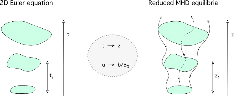
Figure 1.— Schematic of the inverse energy cascade for the solutions of the 2D Euler equation (left panel) and for reduced MHD equilibria (right panel). In the hydrodynamic case (left panel) an eddy of size $\ell$ doubles its size in the eddy-turnover time $t_{\ell}\sim\ell/u_{\ell}$ (Equation [13]). For the structure of reduced MHD equilibria (right panel) this implies (via the mapping $t\rightarrow z$, $\mathbf{u}\rightarrow\mathbf{b}/B_{0}$ given by Equation (10)) that an equilibrium solution with magnetic islands of transverse scale $\ell$ in the plane $z=0$ will acquire an axial asymmetry along the $z$-direction characterized by the variation length-scale $z_{\ell}\sim B_{0}\ell/b_{bd}$ (Equation [14]), since magnetic islands in the plane $z=z_{\ell}$ have an approximately double transverse scale ($\sim 2\ell$).

3.1. Structure of Reduced MHD Equilibria and Dynamics

This phenomenology can be applied to the reduced MHD equilibria (Equation [8]) using the mapping (10), as schematically shown in Figure 1. Eddies, that in the hydrodynamic case are velocity vortices, correspond now to magnetic islands. Then, given a magnetic field $\mathbf{b}_{bd}(x,y)$ at the boundary $z=0$ with energy at scales $\sim\ell$ (i.e., a field structured in magnetic islands of scale $\sim\ell$), the unique and regular equilibrium solution $\mathbf{b}_{eq}(x,y,z)$ with $\mathbf{b}_{eq}(x,y,z=0)=\mathbf{b}_{bd}(x,y)$ is characterized by an increasingly stronger inverse cascade in the x-y planes for higher values of $z$ (see Figure 1, right panel), with the orthogonal magnetic field length-scale $\ell$ getting progressively larger up to doubling its value in the plane

$$z_{\ell}\sim\frac{B_{0}}{b_{bd}}\,\ell,$$ (14)

the analog of the eddy turnover time, derived from Equation (13) using the mapping (10). If the magnetic field is characterized by a scale of order $\ell$ at $z=0$ it will have its energy at scale $\sim 2\ell$ at $z=z_{\ell}$, corresponding respectively to magnetic islands of scales $\ell$ and $2\ell$ in the x-y planes $z=0$ and $z=z_{\ell}$.

Therefore the equilibrium solution $\mathbf{b}_{eq}(x,y,z)$ is generally asymmetric in the axial direction $z$, but it can be almost invariant or have strong variations, depending on the relative value of the length-scale $z_{\ell}$ compared to the loop length $L_{z}$. As long as the variation scale is larger than the loop length ($z_{\ell}>L_{z}$) the field has a weak variation along $z$, but for increasingly smaller values of $z_{\ell}$ ($z_{\ell}<L_{z}$) the field becomes progressively more asymmetric along z due to the inverse cascade. Fixed the value of the guide field $B_{0}$ and the scale of the magnetic field $\ell$, the axial variation scale $z_{\ell}$ is inversely proportional to the magnetic field intensity at the boundary $b_{bd}$: quasi-invariant equilibria are then obtained for weak magnetic fields $b_{bd}$, while increasingly stronger fields result in more asymmetric equilibria.

A strong asymmetry of the magnetic field $\mathbf{b}$ along $z$ is generally not compatible with the dynamical solutions of the reduced MHD equations (1)-(2), as confirmed by nonlinear simulations (for a more detailed discussion of the topics summarized in the present and next paragraph see Rappazzo et al., 2008). The derivatives along $z$ appear only in linear terms in Eqs. (1)-(2). Introducing the Elsässer variables $\mathbf{z}^{\pm}=\mathbf{u}\pm\mathbf{b}$, and neglecting nonlinear and diffusive terms, the remaining linear terms yield the two wave equations:

$$\partial_{t}\mathbf{z}^{\pm}=\pm B_{0}\,\partial_{z}\mathbf{z}^{\pm},\qquad\textrm{with}\qquad\nabla\cdot\mathbf{z}^{\pm}=0.$$ (15)

Thus fluctuations propagate along $z$ at the Alfvén speed $B_{0}$, and a strongly asymmetric field cannot be generated, particularly for the problem considered here with line-tying boundary conditions. For instance a velocity $\mathbf{u}_{ph}$ at the boundary $z=0$ implies the “reflection” condition $\mathbf{z}^{-}=-\mathbf{z}^{+}+2\mathbf{u}_{ph}$ ($\mathbf{z}^{-}$ propagates inward, $\mathbf{z}^{+}$ outward), i.e., generalized Alfvén waves are injected and propagate in the computational box, and only the $m=0$ mode does not propagate in the axial direction.

Considering an initial condition with only the guide field $\mathbf{B}=B_{0}\mathbf{\hat{e}}_{z}$, vanishing orthogonal component $\mathbf{b}=0$, and a constant velocity $\mathbf{u}_{ph}$ at the photospheric boundary that shuffles the magnetic field line footpoints, an orthogonal component of the magnetic field invariant along $z$ is generated and it grows linearly in time as

$$\mathbf{b}(x,y,z,t)=\mathbf{u}_{ph}(x,y)\frac{t}{\tau_{A}},$$ (16)

where $\tau_{A}=L_{z}/B_{0}$ is the Alfvén crossing time in the axial direction. Strictly speaking higher modes are present depending on how the velocity $\mathbf{u}_{ph}$ is turned on, but they represent a small contribution compared to Equation (16) that is the strongly dominant term.

The solution (16) is obtained from Equations (15) (see Rappazzo et al., 2008), thus neglecting nonlinear terms in the reduced MHD equations. This is justified as long as $b$ is small. In fact Rappazzo & Parker (2013) have shown that for initial configurations with only the $m=0$ mode in the axial direction and a non-vanishing 2D orthogonal Lorentz force component (with corresponding term $\mathbf{b}\cdot\nabla j\neq 0$ in Equation [8]), nonlinearity is strongly suppressed, i.e., the nonlinear terms can be neglected, for magnetic fields with intensities below the magnetic threshold $b\sim\ell B_{0}/L_{z}$. The magnetic field decays only for larger magnetic fields $b>\ell B_{0}/L_{z}$, while for smaller values the system does not form significant current sheets and energy is not dissipated.

The intensity threshold $b\sim\ell B_{0}/L_{z}$ corresponds to a critical equilibrium variation length-scale of the order of the loop length $z_{\ell}\sim L_{z}$ (Equation [14]). Since fields with only $m=0$ are invariant along $z$ the correspondent equilibria length-scale $z_{\ell}$ can be computed with $b_{bd}=b$. For $b<\ell B_{0}/L_{z}$ the corresponding equilibrium, i.e., the equilibrium solution computed with $b_{bd}=b$ at the boundary, has $z_{\ell}>L_{z}$ and it is quasi-invariant along $z$. Consequently magnetic fields with $m=0$ and intensity below the intensity threshold $b\sim\ell B_{0}/L_{z}$ are very close to their corresponding equilibrium solution. It is such close proximity to an equilibrium that suppresses nonlinearity, that at equilibrium is indeed entirely depleted.

The emerging phenomenology for the dynamics of initially straight axial field lines shuffled by a velocity field $\mathbf{u}_{ph}$ constant or slowly changing in time (so that the induced magnetic field is quasi-invariant along $z$) is therefore the following: since at first the induced magnetic field is small, the associated variation scale is large $z_{\ell}\gg L_{z}$, nonlinearities are suppressed and the magnetic field grows as in Equation (16) until the variation length-scale becomes smaller than the loop length $z_{\ell}\lesssim L_{z}$, when nonlinearity can develop leading to the formation of current sheets.

The decay of initial configurations with a parallel m=0 mode are relevant for slow photospheric motions. But in general the system has three characteristic timescales:

1. the surface convective timescale $\tau_{sc}\sim(\ell_{sc}/2)/u_{ph}$, essentially the typical lifetime of a granule, approximately given by the ratio of half its length-scale $\ell_{sc}$ over the photospheric velocity $u_{ph}$ (typical values for the Sun are $\ell_{sc}\sim 10^{3}$ km, $u_{ph}\sim 1$km/s, and $\tau_{sc}\sim 5-8$ m),

2. the Alfvén crossing time $\tau_{A}=L_{z}/B_{0}$, where $L_{z}$ is the loop axial length and $B_{0}$ the Alfvén length associated to the guide field, and

3. the nonlinear timescale $\tau_{nl}$, that is investigated theoretically and numerically.

For typical X-ray bright loops $L_{z}\sim 40\times 10^{3}\,$km and $B_{0}\sim 2\times 10^{3}\,$km/s, therefore the Alfvén crossing time $\tau_{A}=L_{z}/B_{0}\sim 20$ s is much smaller than the photospheric timescale, with $\tau_{A}/\tau_{sc}\sim 0.04$. For these loops photospheric motions are then characterized by a low frequency, i.e.,

$$\tau_{sc}\gg\tau_{A},$$ (17)

and a constant (zero frequency, $\tau_{sc}=\infty$) photospheric velocity can be a good approximation, since such slow variation of photospheric motions ($t_{sc}/\tau_{A}\sim 25$) introduces only wavelenghts much longer than the loop length itself along $z$, and the resulting magnetic field (16) can be considered invariant along $z$.

Nevertheless this condition can break down for longer solar coronal loops and for loops on other active stars with outer convective envelopes and magnetized coronae, that exhibit broad variations in magnetic field intensity and topologies (Donati & Landstreet, 2009; Reiners, 2012), and photospheric motion properties (Ludwig et al., 2002; Beeck et al., 2013), for which $\tau_{sc}\sim\tau_{A}$, or $\tau_{sc}<\tau_{A}$. In this case the resulting magnetic field will have a more complex expression than Equation (16), and higher modes along $z$ will be present and contribute increasingly more, the faster the convective timescale $\tau_{sc}$ compared to the Alfvén crossing time $\tau_{A}$.

Therefore the structure of the magnetic field induced in coronal loops by photospheric granulation will be dominated by the $m=0$ mode along $z$ (i.e., the field is quasi-invariant along $z$) for the typical X-ray bright solar loops for which $\tau_{sc}>>\tau_{A}$, while for longer loops (including loops on other active stars) higher modes ($m\geq 1$) will be increasingly more important the smaller the timescale ratio $\tau_{sc}/\tau_{A}<1$.

Table 1Simulations Summary

Run	z-modes	$B_{0}$	numerical grid	$Re_{4}$
A	m=0	103	2D: 5122	$10^{19}$
B	m=0	103	3D: 5122 $\times$ 252	$10^{19}$
C	m=1	103	3D: 5122 $\times$ 252	$10^{19}$
D	m=0–4	103	3D: 5122 $\times$ 252	$10^{19}$

In both cases the variation scale $z_{\ell}\sim\ell B_{0}/b_{bd}$ (Equation [14]) measures the asymmetry of the equilibrium solution. In both cases, even in presence of higher modes $m\geq 1$, the dynamical solutions of the reduced MHD equations will not be asymmetric along $z$, in contrast to the equilibria with $z_{\ell}<L_{z}$.

In the following sections the dynamics of configurations with different initial conditions, with a single mode along $z$ ($m=0$ and $m=1$), and with all modes $0\leq m\leq 4$ excited, are investigated through numerical simulations (see Table 1).

The 2D photospheric velocity $\mathbf{u}_{ph}$ models photospheric motions. These have large scales (with $\ell\sim 10^{3}$ km) and are disordered, since they originate from turbulent convection. Thus generally the magnetic field $\mathbf{b}$ will have a non-vanishing 2D Lorentz force component, i.e., $\mathbf{b}\cdot\nabla j\neq 0$, since the opposite would imply that $j$ should be constant on the field lines of $\mathbf{b}$, a condition too symmetric to apply to turbulent convection (this could be realized, e.g., with an exactly 1D magnetic shear along one direction, or with perfectly circular field lines). Therefore in all simulations presented here the 2D Lorentz force component of the magnetic field does not vanish, i.e., $\mathbf{b}\cdot\nabla j\neq 0$.

Notice that when $\mathbf{b}\cdot\nabla j=0$ we obtain $\partial_{z}j=0$ from the equilibrium Equation (8), hence in this case the variation length-scale is formally infinite $z_{\ell}=\infty$ and it is always larger than the loop length. The inverse cascade picture of the 2D Euler equation described in section 3 is indeed valid only for initial conditions that are out of equilibrium. If $\mathbf{u}\cdot\nabla\omega=0$ in Equation (9) then there is no time evolution and formally $\tau_{\ell}=\infty$ (Equation [13]). Reduced MHD equilibria with $\partial_{z}j=0$ (or equivalently $\mathbf{b}\cdot\nabla j=0$) are those apt to describe classic linear instabilities (such as kink instabilities), and their dynamical accessibility will be discussed in the following sections.

4. Results

The results of the numerical simulations are presented in this section. All simulations, with the exception of Run A, implement line-tying boundary conditions with field line footpoints rooted in a motionless plasma in the photospheric-mimicking planes $z=0$ and $z=L_{z}$. Run A implements periodic boundary conditions in the axial direction $z$, and since its initial condition is invariant along $z$ the dynamics will not introduce any variation along along this direction ($\partial_{z}=0$) and the simulation is restricted to a 2D plane. In the orthogonal directions (x–y) all runs use periodic boundary conditions.

All simulations consider the decay (or equivalently relaxation) of an initial magnetic configuration made of large-scale Fourier modes (as described in Section 2.1) with non-vanishing 2D orthogonal Lorentz force component ($\mathbf{b}\cdot\nabla j\neq 0$). The guide field intensity is $B_{0}=1000$ for all simulations, corresponding to an Alfvén velocity of $1000$ km/s, a typical value for solar coronal loops.

Dissipative simulations with initial conditions made of single parallel modes are described in Sections 4.1 (m=0) and 4.2 (m=1), while in Section 4.3 the initial condition has all modes with $0\leq m\leq 4$. A summary of the simulations is shown in Table 1.

The initial magnetic fields used in these decaying simulations can be considered as “snapshots” of the coronal magnetic field at different stages of its evolution, particularly for the problem of an initially straight field shuffled at its footpoints by photospheric motions [see Equation (16)]. The different parallel modes are related to the photospheric motions frequency, as discussed in the following sections. Additionally the relaxation of magnetic fields is a topic of general and broad interest to solar physics (e.g., Priest, 2014).

4.1. Runs A–B: single mode m=0

This section presents an extended analysis of the dissipative simulations carried out by Rappazzo & Parker (2013) that investigate the decay (or equivalently relaxation) of initial magnetic configurations with an out-of-equilibrium orthogonal magnetic field and parallel mode m=0 (runs A-B).

The initial magnetic field is invariant along $z$ since only the mode m=0 is present. It has the same structure for all runs A-B, with same topology for the magnetic field lines of $\mathbf{b}$, as shown in Figure 4 at time $t=0$, but different values of the orthogonal field intensity rms $b_{0}$ (the proportionality factor in equation [3]) are used. Respect to the guide field $B_{0}$ (same for all runs) the intensity is $b_{0}=0.1\,B_{0}$ for run A, while run B comprises a set of simulations performed with same parameters except $b_{0}$ that spans the range $0.01\leq b_{0}/B_{0}\leq 0.1$.

Runs A and B differ for the boundary conditions along z, periodic for run A and line-tied for runs B. In the periodic case the invariance along $z$ is preserved during the time evolution, therefore for run A Equations (1)-(2) are integrated in a 2D x–y plane with $\partial_{z}=0$.

Periodicity along $z$ is appropriate as a local approximation for the central part of very long loops, where line-tying at the boundary has a weak influence. In particular line-tied forced simulations, with a velocity field at the photospheric-mimicking boundaries, have shown that dynamics resembles those of periodic simulations for low values of the ratio $f_{c}=\ell_{sc}B_{0}/L_{z}u_{ph}$ (Rappazzo et al., 2007, 2008). Fixed the scale of granular cells $\ell_{sc}$ and the photospheric velocity rms $u_{ph}$, line-tying has a weaker impact on longer loops (with larger $L_{z}$) or loops with weaker guide fields (smaller $B_{0}$).

Since the 2D run A is started with an out-of-equilibrium magnetic field ($\mathbf{b}\cdot\nabla j\neq 0$), it is therefore akin to 2D turbulence decay simulations (Hossain et al., 1995; Galtier et al., 1997; Biskamp, 2003) that use similar initial conditions for the magnetic field, but additionally have an initial velocity field in equipartition. The dynamics are nevertheless similar and in the 2D case total energy decays approximately as $E\propto t^{-1}$ (Figure 2, inset), even if the initial velocity vanishes everywhere. Until time $t\sim 0.4\,\tau_{A}$ total energy is conserved, but the non-vanishing Lorentz force transfers $\sim 15\%$ of magnetic energy $E_{M}$ into kinetic energy $E_{K}$, henceforth leading to the formation of small-scales and current sheets, dissipating $\sim 90$% of the initial magnetic energy, while kinetic energy remains much smaller than magnetic energy throughout (Rappazzo & Parker, 2013).

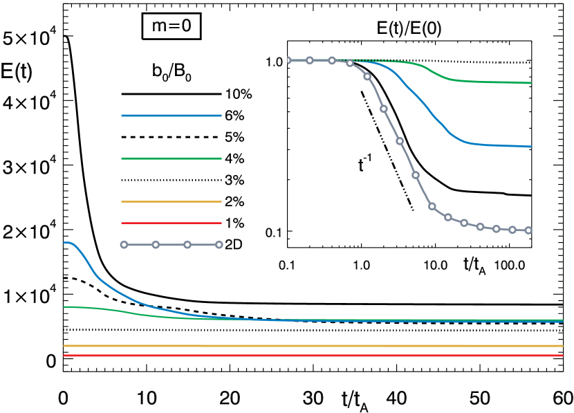
Figure 2.— Runs A–B (m=0): Total energy vs. time for line-tied simulations with different values of $b_{0}/B_{0}$ (runs B) and the 2D simulation (run A, with $b_{0}/B_{0}=10\%$). The inset shows in logarithmic scale total energy normalized with its inital value.

In Fourier space magnetic energy has initially only large-scale perpendicular modes k=3 and 4 (Figure 3, top panel). As nonlinearity develops energy is progressively transferred toward both small (direct) and large scales (inverse cascade). In physical space the direct cascade gives rise to current sheets (Figure 4, top row) that enable dissipation through magnetic reconnection. As dissipation peaks at $t\sim 1.7\,\tau_{A}$, the spectrum extends fully toward high wave-numbers exhibiting an approximate $k^{-5/3}$ power-law. At the same time a substantial fraction of total energy has already been transferred to large-scale modes k=1 and 2 through the inverse cascade, that in physical space corresponds to the coalescence of magnetic islands as magnetic reconnection occurs. As dynamics proceeds the energy transferred at the small scales is dissipated leading to the disappearance of current sheets and small-scales, so that the system finally relaxes to a state with energy mostly at large scales (particularly in mode k=1), corresponding in physical space to large-scale magnetic islands and large-scale current layers (Figure 4, top row, $t\sim 210\,\tau_{A}$). The whole process is akin to Taylor relaxation (Taylor, 1986) and self-organization leading to the formation of large-scale structures (Hasegawa, 1985).

In the 2D case (run A) solutions differing only for the value of $b_{0}$ (the rms of the initial magnetic field in Equation [3]) have a self-similar structure. Indicating with $\psi_{0}(\mathbf{x},t)$ and $\varphi_{0}(\mathbf{x},t)$ the solution of Equations (1)-(2) with initial magnetic field rms $b_{0}$, then the solutions with $b^{\prime}_{0}=\sigma b_{0}$, and same random amplitudes in Equation (3), are given by:

$$\psi^{\prime}(\mathbf{x},t)=\sigma\,\psi_{0}(\mathbf{x},\sigma t),\qquad\varphi^{\prime}(\mathbf{x},t)=\sigma\,\varphi_{0}(\mathbf{x},\sigma t),$$ (18)

as can be verified by direct substitution. Consequently all these solutions have a similar structure and their time evolution differs only for the scaling factor $\sigma$. In particular if current sheets form for a certain value of $b_{0}$, they will always do for any value of $b_{0}$ at scaled times. Analogously energy will exhibit a power-law decay with the same exponent because $E^{\prime}(t)=\sigma^{2}E_{0}(\sigma t)$, implying that if $E(t)\propto t^{-\alpha}$ then $E^{\prime}(t)\propto t^{-\alpha}$.

When the same initial condition is used with line-tying boundary conditions, the system is no longer invariant along $z$, as now the velocity must vanish at the top and bottom plates $z=0$ and $z=L$, therefore the velocity cannot develop uniformly along z as in the periodic case.

The time evolution of total energy for line-tied simulations with different values of $b_{0}$ is shown in Figure 2. While the dynamics of the system with $b_{0}/B_{0}=10\%$ is similar to the 2D case with energy dissipating $\sim 84\%$ of its initial value, the behavior is increasingly different for lower values of $b_{0}$, with progressively less energy getting dissipated. For $b_{0}/B_{0}\lesssim 3\%$ no significant energy dissipation nor decay are observed. Additionally, also for the decaying cases their dynamics are strongly suppressed once energy crosses this threshold. As shown in Fig. 2 no energy decay is observed below $E\sim 5\times 10^{3}$, corresponding to a ratio $\langle b^{2}\rangle^{1/2}/B_{0}\sim 3\%$. The inset in Fig. 2 shows that energy decays with different power-law indices for lower values of $b_{0}/B_{0}$, hence time self-similarity is lost and the impact of line-tying on the dynamics is more complex than a simple delay as in the 2D case (Equations [18]).

Magnetic energy spectra (integrated along $z$, Figure 3) show similar dynamics for the 2D (top panel) and the 3D case with $b_{0}/B_{0}=10\%$ (middle panel). In particular the spectra are fully extended toward the small scales as dissipation occurs, corresponding to the formation and dissipation of current sheets in physical space (Figure 4, second row). While similar behavior is observed for magnetic field intensities $b_{0}>3\%$, below this threshold the spectra do not extend to the high wave-numbers where energy gets dissipated (Figure 3, bottom panel, $b_{0}/B_{0}=2\%$), i.e., current sheets do not thin below the critical diffusive thickness that allows magnetic reconnection and energy dissipation to occur. As shown in Figure 4 at the peak of dissipation (central column) both current maxima and the number of current sheets decrease for smaller $b_{0}/B_{0}$, and for $b_{0}/B_{0}=2\%$ no current sheets are formed, but only a few ripples are visible in the magnetic field (enhanced in the current) and are eventually dissipated on long timescales.

Figure 3.— Runs A–B (m=0): Magnetic energy spectra (integrated along $z$) at selected times for the 2D run A with $b_{0}/B_{0}=10$% (top panel), and for run B simulations with $b_{0}/B_{0}=10$% (middle) and $b_{0}/B_{0}=2$% (bottom). Energy is normalized with its initial value at time t=0, when energy is present only at perpendicular modes $k=3$ and 4 (diamond symbol). Spectra at the time of maximum dissipation for each simulation are drawn in a continuous line.

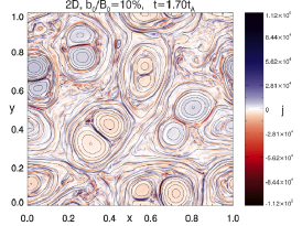
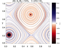
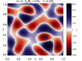
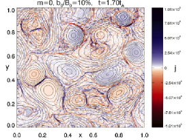
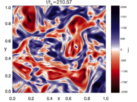
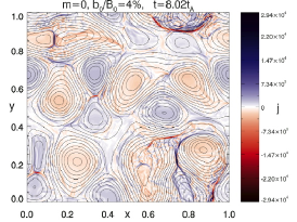
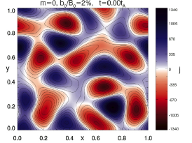
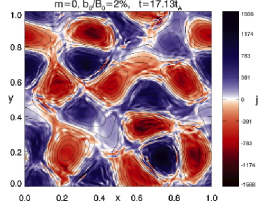
Figure 4.— Runs A–B (m=0): Magnetic field lines of the orthogonal magnetic field component $\mathbf{b}$ and current density $j$ at selected times. Top row shows snapshots from the 2D simulation (run A), while snapshots from three 3D simulations (run B) with different ratios $b_{0}/B_{0}$ are shown in the remaining rows (in this case the mid-plane $z=5$ is considered). The first column shows the initial condition at $t=0$, same for all except for the ratio $b_{0}/B_{0}$, the second column shows the fields at the time of maximum dissipation, while the third column shows the fields at a later time when the fields have relaxed and little if any energy dissipation occurs.

Furthermore, spectra show that the inverse energy cascade decreases from the 2D to the 3D case with $b_{0}/B_{0}=10\%$, in fact while in the asymptotic state of the 2D run ($t=210\,\tau_{A}$) most of the energy is in the $k=1$ mode and higher modes are much smaller, in the 3D case the mode $k=2$ has the higher value. For 3D simulations with smaller $b_{0}/B_{0}$ the inverse cascade is progressively fainter and does not occur for $b_{0}/B_{0}\lesssim 3\%$, as shown in Figure 3 (bottom panel) for $b_{0}/B_{0}=2\%$, where no significant energy is found in perpendicular modes smaller ($k\leq 2$) than those present at time $t=0$ ($k=3$, $4$).

In physical space (Figure 4) the inverse cascade corresponds to larger-scale magnetic islands in the asymptotic state. Since a larger fraction of magnetic energy is dissipated for higher values of $b_{0}/B_{0}$ and in the 2D case, more magnetic flux is reconnected, thus leading to increased coalescence and larger magnetic islands. Additionally the field line topology in the relaxed state is substantially unaltered respect to the initial condition for $b_{0}/B_{0}\lesssim 3\%$ (cf. the first and last columns in Figure 4), with higher variations for higher values of $b_{0}/B_{0}$ and most of all in the 2D case.

A key difference distinguishes the 2D and 3D asymptotic topologies. Although all simulations are started with a non-vanishing 2D Lorentz force component ($\mathbf{b}\cdot\nabla j\neq 0$), the 2D simulation relaxes to an approximate equilibrium with $\mathbf{b}\cdot\nabla j=0$, but all 3D simulations relax to an orthogonal field with $\mathbf{b}\cdot\nabla j\neq 0$, regardless of how much energy is dissipated during the decay (none for $b_{0}/B_{0}=2\%$, and an 84% energy decay for the $b_{0}/B_{0}=10\%$ run B). Further analysis is presented in the following to understand the nature of these equilibria and how they are approached.

In the 2D case the equilibrium condition (8) becomes simply $\mathbf{b}\cdot\nabla j=0$. This requires the current density $j$ to be constant along the field lines of $\mathbf{b}$ (or equivalently that the isosurfaces of $j$ are also isosurfaces of the magnetic potential $\psi$). This condition is generally satisfied only in highly symmetric configurations such as one-dimensional magnetic shears, e.g., $\mathbf{b}=f(y)\,\mathbf{\hat{e}}_{x}$, or rotationally invariant fields as $\mathbf{b}=f(r)\,\mathbf{\hat{e}}_{\theta}$ ($f$ is a generic function in cartesian or cylindrical coordinates). In the 2D case the field lines are mostly circular in the asymptotic state (Figure 4) and the isosurfaces of the current density and of the magnetic potential (the field lines of $\mathbf{b}$) overlap. In the 3D case the full equilibrium equation (8) has to be considered, and the fact that for run B with $b_{0}/B_{0}<3\%$ no significant dynamics occurs with the initial orthogonal magnetic field essentially unaltered even though its 2D Lorentz force does not vanish, i.e., $\mathbf{b}\cdot\nabla j\neq 0$, implies that $\partial_{z}j$ increases only slightly from its initial vanishing value.

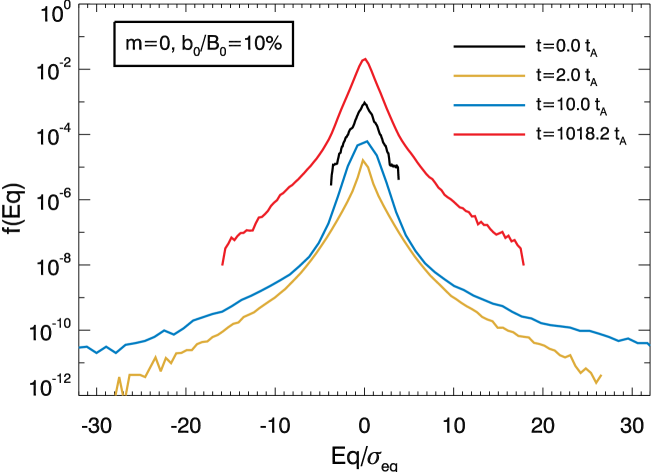
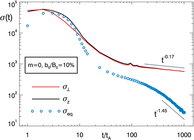
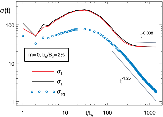
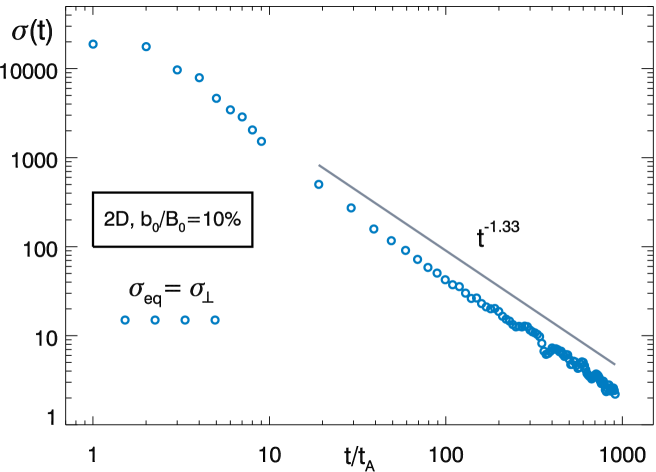
Figure 5.— Runs A–B (m=0): Probability density functions (PDFs) of the reduced MHD equilibrium equation (8) at selected times for the run B with $b_{0}/B_{0}=10\%$ (top panel), shown in a semi-log plot. To accommodate the large variation of the standard deviation the abscissa displays the values normalized with the standard deviation at the corresponding time. The remaining panels display in logarithmic scale the standard deviations as a function of time for the 2D simulation (bottom panel) and the 3D runs B with $b_{0}/B_{0}=2\%$ and $10\%$ (middle panels). For the 3D cases the orthogonal ($\sigma_{\perp}$), parallel ($\sigma_{z}$) and total ($\sigma_{eq}$) standard deviations are shown.

The dynamical approach of the system to equilibrium is further investigated with the probability density functions (PDFs) of the equilibrium equation terms. These PDFs are histograms of the quantities of interest normalized so that the resulting function $f(q)$ multiplied by the bin size $\Delta q$ gives the fraction of points in the computational box where the specific quantity $q$ has its value in the interval $[q-\Delta q/2,q+\Delta q/2]$, and the integral $\int\mathrm{d}qf(q)=1$. PDFs have been computed for both the left and right hand terms in the equilibrium equation (8), and for their difference, indicated with

$$Eq(\mathbf{x})=\frac{\partial j}{\partial z}+\frac{\mathbf{b}\cdot\nabla j}{B_{0}}.$$ (19)

This is a three-dimensional scalar function that measures how far the system is from equilibrium locally at point $\mathbf{x}$, vanishing at equilibrium and with higher absolute values the larger the departure from equilibrium. The PDFs have been computed for all the simulations with $m=0$ (for the 2D case only the term $\mathbf{b}\cdot\nabla j/B_{0}$ is present), and they all exhibit similar behavior. All these PDFs have vanishing averages, therefore their standard deviations can be defined as:

$$\sigma_{z}=\left\langle\left(\frac{\partial j}{\partial z}\right)^{2}\right\rangle^{1/2},\qquad\sigma_{\perp}=\left\langle\left(\frac{\mathbf{b}\cdot\nabla j}{B_{0}}\right)^{2}\right\rangle^{1/2},$$ (20)

$$\sigma_{eq}=\left\langle\left(\frac{\partial j}{\partial z}+\frac{\mathbf{b}\cdot\nabla j}{B_{0}}\right)^{2}\right\rangle^{1/2},$$ (21)

respectively for the first and second terms and the whole Equation (19), labeled as parallel ($\sigma_{z}$), orthogonal ($\sigma_{\perp}$) and total ($\sigma_{eq}$).

In Figure 5 (top panel) the PDFs of the equilibrium function $Eq(\mathbf{x})$ are shown in a semi-log plot at selected times for run B with $b_{0}/B_{0}=10\%$. The abscissa is rescaled with the standard deviation of the PDFs to improve visualization, since they exhibit large variations in time. The PDF of $Eq$ is generally super-Gaussian (with a peak around zero and “tails” farther out), particularly close to maximum dissipation time ($t=2\,\tau_{A}$), however the central part appears closer to a Gaussian distribution at later times ($t=10\,\tau_{A}$), and particularly in the final asymptotic stage ($t=1018.2\,\tau_{A}$). Although long tails are present at most times, in all cases $\sim 95\%$ of points lies within two standard deviations from zero (from $94\%$ at $t=0$ to $96\%$ at $t=10\,\tau_{A}$).

An appropriate quantitative measure of the distance of the system from equilibrium is given by the standard deviation of $Eq$, shown in the mid panels of Figure 5 along with $\sigma_{z}$ and $\sigma_{\perp}$ for runs B with $b_{0}/B_{0}=2\%$ and $10\%$. In this case, since their averages vanish, the standard deviations are also the rms of the considered quantities. At time $t=0$ the derivative along $z$ of $j$ vanishes ($\partial_{z}j=0$) so that initially $\sigma_{z}=0$ for both runs, while $\sigma_{\perp}=25.32$ and $633.09$ respectively. But already after one Alfvén time $\tau_{A}$ they both increase (substantially only for the run with $b_{0}/B_{0}=10\%$) reaching similar values $\sigma_{z}\sim\sigma_{\perp}$, and subsequently continue to be very close while their values decrease. The rms of the equilibrium function $Eq$, the standard deviation $\sigma_{eq}$, decreases with time, and it is asymptotically smaller than $\sigma_{z}$ and $\sigma_{\perp}$. As shown in Figure 5 all standard deviations decrease asymptotically like a power-law with $\sigma_{z}\sim\sigma_{\perp}\propto t^{-\alpha}$, where spectral indices are respectively $\alpha=0.17$ and $0.038$ for the runs with $b_{0}/B_{0}=10\%$ and $2\%$, while the rms of $Eq$ decays at a faster rate with $\sigma_{eq}\propto t^{-\beta}$, where $\beta=1.45$ and $1.25$.

This implies that while the rms of $\partial_{z}j$ and $\mathbf{b}\cdot\nabla j/B_{0}$ have about the same value and remain approximately constant in the asymptotic state (when their power-law decay occurs), equilibrium is approached as the two terms in Equation (19) balance each other progressively more throughout the computational box, thus leading to the rapid decrease of $\sigma_{eq}$.

The initial increase of the standard deviations is larger for $b_{0}/B_{0}=10\%$ than for the $2\%$ case, since for $b_{0}/B_{0}=10\%$ the system is farther out of equilibrium in the beginning, with strong currents forming quickly and maximum dissipation rate occurring at $t\sim 1.7\,\tau_{A}$, when also standard deviations approximately peak. Their subsequent decrease up to $t\sim 20\,\tau_{A}$ is enhanced by the strong decay of magnetic energy and progressive disappearance of current sheets, before approaching the asymptotic stage around $t\sim 200\,\tau_{A}$. Although the standard deviations for run B with $b_{0}/B_{0}=2\%$ have similar behavior to the case with $b_{0}/B_{0}=10\%$, their variations are much smaller, since the field just undergoes a slight adjustment, without any significant energy decay (Figure 2), current sheets formation or significant change in the magnetic field topology (see bottom row in Figure 4).

For the 2D run A there is no parallel standard deviation $\sigma_{z}$. The rms of $Eq$, $\sigma_{eq}$, is equal to $\sigma_{\perp}$, and similarly to runs B its time evolution follows the power-law $\sigma_{eq}\propto t^{-\beta}$ with $\beta=1.33$, as shown in Figure 5 (bottom panel). It is worth mentioning that $\sigma_{eq}$ initially grows larger respect to its initial value ($=633$) for run B respect to run A with same $b_{0}/B_{0}=10\%$. The reaction of the line-tied field sets the system further out of equilibrium, an enhancement of nonlinearity that might favor the development of singularities in the line-tied system respect to the periodic case.

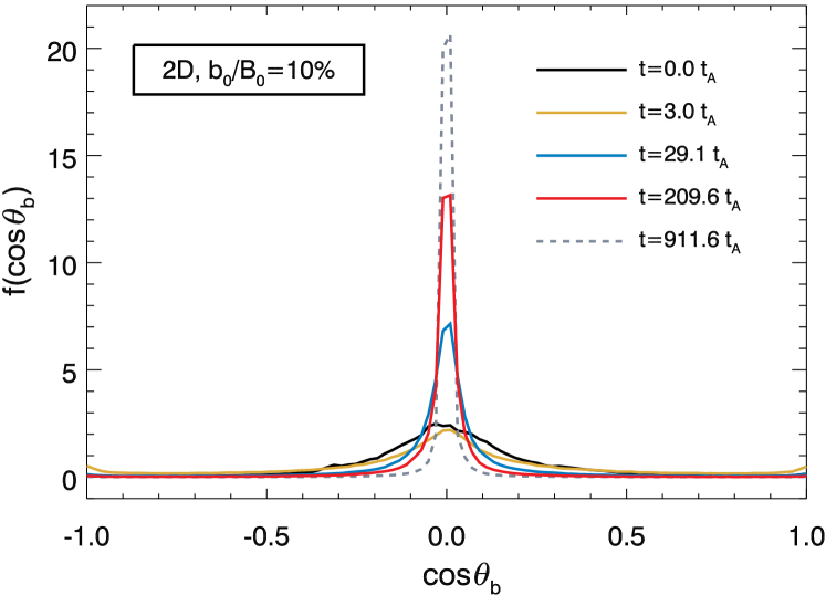
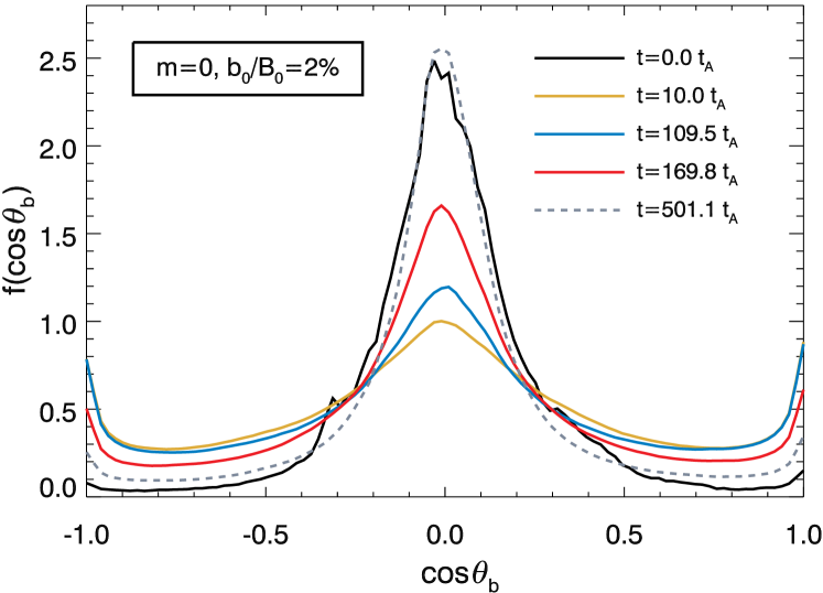
Figure 6.— Runs A–B (m=0): Probability density functions (PDFs) of the angle $\theta_{b}$ between the orthogonal magnetic field $\mathbf{b}$ and the current density gradient $\nabla j$ at selected times for the 2D run A with $b_{0}/B_{0}=10\%$ (top panel), and the 3D runs B with respectively $b_{0}/B_{0}=10\%$ (middle) and $b_{0}/B_{0}=2\%$ (bottom).

Further insight into the dynamics is gained analyzing the probability density function of the cosine of the angle $\theta_{b}$ between $\mathbf{b}$ and $\nabla j$

$$\cos\theta_{b}=\frac{\mathbf{b}\cdot\nabla j}{|\mathbf{b}|\,|\nabla j|},$$ (22)

shown in Figure 6. At time t=0 the “2D perpendicular” Lorentz force term does not vanish for all simulations ($\mathbf{b}\cdot\nabla j\neq 0$). Since the orthogonal component of the magnetic field differs for runs A–B only for a proportionality factor (Equation [3]), the PDF is the same for all runs A–B (e.g., see mid-panel in Figure 6). Although it is peaked around zero (corresponding to the 2D equilibrium condition $\mathbf{b}\cdot\nabla j=0$) it spreads out with significant values up to $|\cos\theta_{b}|\lesssim 1/2$, corresponding to an approximate $60^{\circ}$ angle around $\theta_{b}=90^{\circ}$. For the 2D run A with $b_{0}/B_{0}=10\%$ (top panel) the PDF initially spreads out during the strongest part of the nonlinear stage ($1\lesssim t/\tau_{A}\lesssim 10$) during which $\sim 90\%$ of the initial energy is dissipated, but afterward peaks progressively more strongly around zero, corresponding to the equilibrium condition for the orthogonal field $\mathbf{b}\cdot\nabla j=0$, with respectively 71% and 96% of the grid points in the volume in the region $|\cos\theta_{b}|<0.1$, spanning an angle of $\sim 11.5^{\circ}$ around $\theta_{b}=90^{\circ}$, at times t=29.1 and $911.6\,\tau_{A}$. This confirms that the system approaches asymptotically an equilibrium with $\mathbf{b}\cdot\nabla j=0$ corresponding in physical space to increasingly circular field lines progressively more coincident with the isosurfaces of $j$, as shown in Figure 4 (top row).

In contrast the picture is radically different for the line-tied simulations. As shown in the middle panel of Figure 6, for run B with $b_{0}/B_{0}=10\%$ the PDF spreads increasingly further out during the time evolution, flattening considerably already after one Alfvén time and remaining flat throughout the subsequent evolution, when $\sim 80\%$ of magnetic energy is dissipated, and in the following asymptotic regime, with peaks forming in correspondence of alignment between the two fields ($\theta_{b}\sim 0^{\circ}$, $180^{\circ}$). Therefore, in contrast with the periodic case (2D run A) the orthogonal magnetic field does not approach the asymptotic equilibrium with $\mathbf{b}\cdot\nabla j=0$ (that would imply also $\partial_{z}j=0$ in the 3D case, Equation [8]), instead in the 3D line-tied case the orthogonal component of the magnetic field remains with a non-vanishing “2D perpendicular” Lorentz force term ($\mathbf{b}\cdot\nabla j\neq 0$).

Furthermore, if the initial magnetic field intensity is below the threshold set out by Rappazzo & Parker (2013), as shown in the bottom panel of Figure 6 for run B with $b_{0}/B_{0}=2\%$, the PDF starts flattening out to some extent but then bounces back very close to its initial profile, corresponding to a slight readjustment of the magnetic field as shown in Figure 4 (bottom row), with the orthogonal magnetic field preserving its non-vanishing perpendicular Lorentz force.

The results of the numerical simulations analyzed in this section are consistent with the heuristic phenomenology laid out by Rappazzo & Parker (2013) and the more refined analysis of the structures of the equilibria expounded in Section 3. The asymmetry along $z$ of the solutions of the reduced MHD equilibrium equation (8) can be estimated with the axial variation length-scale $z_{\ell}\sim\ell B_{0}/b$ (Equation [14], see also Figure 1), where $\ell$ is the perpendicular characteristic scale (in the $x$–$y$ plane) of the magnetic field component $\mathbf{b}$.

As discussed in Section 3.1, the dynamical solutions of the reduced MHD equations (1)-(2) generally cannot exhibit strong asymmetries along $z$, in particular when driven from the photospheric boundaries. On the other hand the equilibria can be strongly asymmetric or quasi-invariant along z, depending on the relative value of the axial variation scale $z_{\ell}$ respect to the loop axial length $L_{z}$, with the critical length given by $z_{\ell}\sim L_{z}$. For small values of $b$ the axial variation scale $z_{\ell}$ is longer than the loop length $L_{z}$ and the corresponding equilibrium solution is quasi-invariant along $z$, while for larger values of $b$ the axial scale $z_{\ell}$ is smaller than the loop length and the equilibrium is more asymmetric along $z$ the larger the magnetic field intensity $b$.

As shown in Figure 2 no substantial energy is dissipated for 3D runs with $b_{0}/B_{0}\lesssim 3\%$, and just minimal dynamics occurs as the field slightly readjusts (Figures 3–6). Since the initial magnetic field (Equation [3]) has a perpendicular scale $\ell\sim L_{\perp}/3.87\sim 1/3.87$ (the averaged wavenumber of the initial condition is 3.87 and $L_{\perp}=1$), this threshold corresponds to a variation length-scale for the initial magnetic field of about $z_{\ell}=\ell B_{0}/b_{0}\gtrsim 100/(3\times 3.87)$, i.e., $z_{\ell}\gtrsim L_{z}$ since $L_{z}=10$.

Therefore for $b_{0}/B_{0}\lesssim 3\%$ the corresponding equilibria, computed from Equation [8] with $\mathbf{b}_{eq}$($z$=0) = $\mathbf{b}_{0}$($z$=0), as described in Section 3, have a large variation length-scale $z_{\ell}\gtrsim L_{z}$ and are therefore quasi-invariant along $z$. Since the initial condition has only the parallel m=0 mode it is invariant along $z$, and therefore very close to the corresponding equilibrium, so that nonlinearity is strongly depleted and only a slight readjustment of the field occurs, with no significant energy dissipation. On the contrary for initial conditions with $b_{0}/B_{0}>3\%$ the corresponding equilibria have smaller variation length-scales $z_{\ell}<L_{z}$, hence the equilibrium solution is strongly asymmetric along $z$, differing substantially from the initial condition that is then necessarily out-of-equilibrium, as shown by the subsequent dynamics and energy dissipation.

Furthermore, as shown in Figure 2, also in the cases when decay occurs, i.e., for initial conditions with $b_{0}/B_{0}>3\%$, the magnetic field relaxes to a new equilibrium that approximately satisfies the condition $b/B_{0}\sim 3\%$ and $z_{\ell}\sim L_{z}$. But while the asymptotic energy of the runs with $b_{0}/B_{0}=4\%$, 5% and 6% are approximately the same, corresponding to a ratio $b/B_{0}\sim 3.3\%$, the run with $b_{0}/B_{0}=10\%$ relaxes to a slightly higher energy with $b/B_{0}\sim 4\%$. On the other hand the run with $b_{0}/B_{0}=10\%$ has a stronger inverse cascade (Figure 3), with significantly larger magnetic islands in the asymptotic regime (Figure 4) and average wavenumber $\sim 2.7$ thus obtaining again $z_{\ell}\sim L_{z}$. When a strong inverse cascade occurs the formation of larger perpendicular scales ($\ell$) increases the value of the axial variation length-scale $z_{\ell}\sim\ell B_{0}/b$, thus attaining the equilibrium condition $z_{\ell}\sim L_{z}$ with a larger value of $b$, and consequently a smaller dissipation of energy.

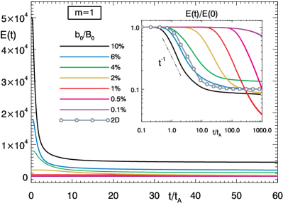
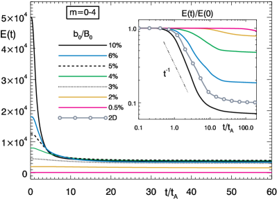
Figure 7.— Runs C (m=1) and D (m=0–4): Total energy vs. time for line-tied simulations with different values of $b_{0}/B_{0}$ for run C with single parallel mode m=0 (left panel) and run D with m=1 (right panel). The 2D run A with $b_{0}/B_{0}=10\%$ is added for comparison. The insets show in logarithmic scale total energies normalized with their initial values.

The critical variation length-scale $z_{\ell}$ origins from a balance of forces because the reduced MHD equilibrium equation (8) represents a balance between two force terms. In the reduced MHD limit (e.g., Montgomery, 1982) the Lorentz force splits into two terms with components only in the orthogonal $x$–$y$ planes: the “perpendicular” ($\mathbf{b}\cdot\nabla\mathbf{b}$) and “parallel” ($B_{0}\partial_{z}\mathbf{b}$) field line tensions (plus the pressure term, determined through the incompressibility condition). The first term represents the field line tension of the orthogonal component $\mathbf{b}$, the only one present in the 2D limit. The second is an additional tension term due to the presence of the guide field $B_{0}$, linked to the tension of the field lines of the total magnetic field $B_{0}\mathbf{\hat{e}}_{z}+\mathbf{b}$. An equilibrium is attained only when these two counteracting components of the Lorentz force balance each other satisfying Equation (8). As outlined in Rappazzo & Parker (2013) these two forces are of the same order of magnitude for the critical intensity

$$b\sim\frac{\ell B_{0}}{L_{z}},$$ (23)

corresponding to the critical axial variation length-scale $z_{\ell}\sim\ell B_{0}/b_{\ell}\sim L_{z}$ as discussed in Section 3.1.

Initially also the 3D line-tied system starts to behave as in the 2D case, with the tension of perpendicular field lines creating an orthogonal velocity, that coupled with all others nonlinear terms are the only ones that can cascade energy and generate current sheets. But this displaces the total line-tied (axially directed) field lines, that now cannot be freely convected around as in the periodic case because of the line-tying constraint at the boundaries, and is then counteracted by the enhanced axial tension that resists bending. Magnetic fields with intensities smaller than the threshold (23) a small variation of $\mathbf{b}$ along $z$ (corresponding to a variation scale larger than the loop length $L_{z}$) is enough to reach an equilibrium, but for intensities larger than of $b\gtrsim\ell B_{0}/L_{z}$ current sheets must form and energy dissipate in order to reach the physically accessible equilibria with $b\sim\ell B_{0}/L_{z}$, since for larger magnetic field intensities the equilibria are strongly asymmetric along $z$ and therefore physically inaccessible.

The analysis in this section has considered exclusively initial conditions invariant along the $z$-direction, with only the parallel mode m=0. In the following sections we extend it to include field variations along $z$ with higher parallel modes..

4.2. Runs C: single mode m=1

The finite length of coronal loops renders the system akin to a resonant cavity. A forcing velocity with frequency $\nu$ at the photospheric boundary, e.g.,

$$\mathbf{u}(x,y,z=L,t)=\mathbf{u}_{ph}(x,y)\cos(\omega t),$$ (24)

where $\omega=2\pi\nu$ is the angular frequency, will inject Alfvén waves at that frequency propagating in the axial direction of the loop. In general these waves, that are continuously injected and reflected at the boundaries (see Section 3.1, Equation [15]), will be out of phase and decorrelated along the loop so that their sum will remain limited the whole time to values of the order of the forcing velocity at the boundary, with no growth in time for the amplitude of the resulting velocity and magnetic fields. But for the resonant frequencies

$$\nu_{n}=n\,\nu_{A}/2,\quad\textrm{with}\quad n\in\mathbb{N}$$ (25)

and $\nu_{A}=1/\tau_{A}$, the waves are in phase and they sum coherently (Ionson, 1985). Thus the magnetic and velocity fields in the loop grow linearly in time similarly to the case with constant velocity (Equation [16]). For instance, considering the boundary velocity (24) at the resonant frequency $\nu_{n}$ with $n\geq 1$, the resulting fields grow approximately as (Einaudi & Velli, 1999; Rappazzo, 2006; Chiuderi & Velli, 2015):

$$\mathbf{b}\sim\mathbf{u}_{ph}\cos\left(\omega_{n}\frac{z}{v_{A}}\right)\cos(\omega_{n}t)\,\frac{t}{\tau_{A}},$$ (26)

$$\mathbf{u}\sim\mathbf{u}_{ph}\sin\left(\omega_{n}\frac{z}{v_{A}}\right)\sin(\omega_{n}t)\,\frac{t}{\tau_{A}}.$$ (27)

Indeed a constant velocity can be regarded as the zero frequency resonance $n=0$ of the system, that differs from resonances with $n\geq 1$ because while the magnetic field grows linearly in time, for $n=0$ the velocity field does not grow and its value remains of the same order of magnitude of the photospheric velocity ($u\sim u_{ph}$).

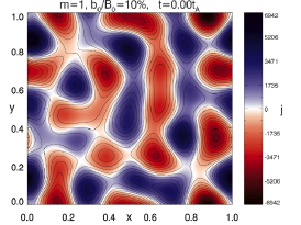
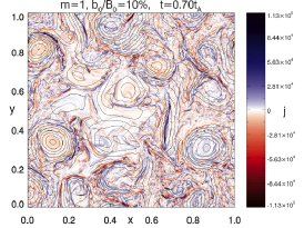
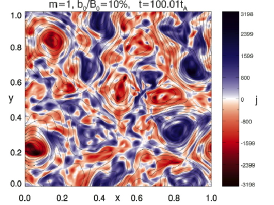
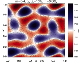
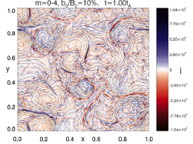
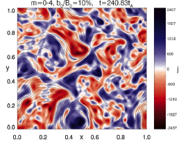
Figure 8.— Runs C (m=1) and D (m=0–4): Magnetic field lines of the orthogonal magnetic field component $\mathbf{b}$ and current density $j$ in the mid-plane $z=5$ at selected times for runs C (top row) and D (bottom row) with $b_{0}/B_{0}=10\%$. The left panels show the initial condition at $t=0$, the central panels show the fields at the time of maximum dissipation, while the right panels show the fields at a later time when they have relaxed (asymptotic regime).

As mentioned in Section 3.1, for X-ray bright solar coronal loops photospheric motions have a low frequency, giving rise to a coronal magnetic field dominated by the parallel $m=0$ mode, and their low frequency can then be approximated with zero. In general photospheric motions characterized by a surface convective timescale $\tau_{sc}$ will not have a single harmonic at the frequency $1/\tau_{sc}$, rather the amplitude of its Fourier transform will peak at the frequency $1/\tau_{sc}$ but include many other harmonics.

For longer loops (with longer Alfvén crossing times $\tau_{A}=L_{z}/v_{A}$ comparable or longer than granulation timescales), and for loops on other active stars with magnetized coronae and outer convective envelopes, photospheric motions can have frequencies closer to resonances higher than $\nu_{0}=0$. Furthermore also when photospheric motions have a dominant low frequency, higher frequency modes will be present, although with smaller amplitudes (Nigro et al., 2008) that contribute considerably less heating (Milano et al., 1997). In all these cases photospheric motions will give rise to parallel modes higher than zero ($m\geq 1$) for the coronal magnetic field. These will be the dominant modes when the photospheric frequency is resonant, and give a small contribution to the magnetic field when photospheric motions frequencies are close to zero. Additionally higher parallel modes can also be generated by nonlinear dynamics also when starting with a zero parallel mode (Buchlin & Velli, 2007), and by disturbances stemming from chromospheric dynamics (De Pontieu et al., 2007).

It is therefore of interest to consider initial conditions with modes higher than $m=0$, and in the numerical simulations analyzed in this section the initial magnetic field has only the parallel mode $m=1$ (corresponding to the resonant frequency $\nu_{2}=\nu_{A}$), while large-scale perpendicular modes are set as in previous simulations with wavenumbers between 3 and 4 (Section 2.1, Equation [3]). Thus unlike run B with $m=0$, the out-of-equilibrium initial magnetic field now varies also along $z$, with both terms in the equilibrium equation (8) not vanishing ($\partial_{z}j\neq 0$, $\mathbf{b}\cdot\nabla j\neq 0$). The magnetic field lines of the orthogonal component $\mathbf{b}$ and current density $j$ are shown in Figure 8 (top row) at time $t=0$ in the mid-plane $z=5$, while isosurfaces of the magnetic potential at $t=0$ are shown in Figure 9 (central column). In both figures the case with $b_{0}/B_{0}=10\%$ is considered. This is one of a series of simulations collectively labeled as runs C, with same parameters for the initial condition except the magnetic field intensity $b_{0}$ (the multiplicative factor in Equation [3]) that spans the range $0.1\%\leq b_{0}/B_{0}\leq 10\%$.

The time evolution of total energy for runs C with different values of $b_{0}$ is shown in Figure 7 (left panel). The run with $b_{0}/B_{0}=10\%$ has a similar behavior to run B with same magnetic field intensity (cf. Figure 2). Its energy decays approximately as $E\propto t^{-1}$, with current sheets forming in physical space (Figure 8, top row) and dissipating $\sim 92\%$ of the initial energy, a slightly higher value respect to the corresponding run B. Subsequently the system relaxes to an asymptotic state with $b/B_{0}\sim 2.87\%$.

The analysis of the equilibria set forth in Section 3.1 shows that the only dynamically accessible equilibria are those with variation length-scale greater than approximately the loop length $z_{\ell}\gtrsim L_{z}$. These have structures very elongated in the axial direction, and therefore dominated by the parallel mode $m=0$. When initial conditions do not include the $m=0$ mode, their higher modes will necessarily have to transfer part of their energy to the mode $m=0$ via nonlinear dynamics in order to relax to equilibrium. Furthermore most of the energy of the modes with $m\geq 1$ that is not converted into the parallel zero mode must be dissipated for the relaxed state to be close to a reduced MHD equilibrium with $z_{\ell}\gtrsim L_{z}$, with a predominant parallel zero mode.

In fact the isosurfaces of the magnetic potential $\psi$ in Figure 9 show that both runs B and C with $b_{0}/B_{0}=10\%$ (respectively in the left and central columns) relax to a lower energy state with structures very elongated along $z$ (the computational box has been rescaled for an improved visualization, but the axial length is ten times longer that the perpendicular cross section length), even though their initial conditions are radically different, consisting exclusively of mode $m=0$ for run B and $m=1$ for run C.

Consequently similar dynamics will occur for all runs C independently from the value of $b_{0}/B_{0}$, as shown in Figure 7, because all of them do not have a mode $m=0$ in their initial magnetic field. Thus they all decay while part of the energy initially in the $m=1$ mode is either transferred to the $m=0$ mode (and partially also to higher order modes) or dissipated (including dissipation of the higher order modes generated during the nonlinear dynamics). On the contrary when the initial condition is made only of mode $m=0$, the system is very close to an equilibrium for $b_{0}/B_{0}\lesssim 3\%$ (runs B, Figure 2) since this condition implies $z_{\ell}\gtrsim L_{z}$ and the magnetic field is quasi-invariant along $z$, so that no substantial dynamics occur when $b_{0}/B_{0}\lesssim 3\%$.

Figure 7 shows that for runs C energy starts decaying at later times for smaller values of $b_{0}/B_{0}$. The longer timescales for dissipation to occur and energy to start decaying is consistent with the decrease of the strength of nonlinear interactions for lower values of $b_{0}/B_{0}$. For instance the eddy turnover time increases as $t_{\ell}\sim 2\ell/b_{0}$, since no velocity is initially present and this soon becomes of the order of $b_{0}/2$ (because for resonant frequencies velocity is in equipartition with the magnetic field). Subsequently velocity strongly decreases once a zero mode is created and the system relaxes.

Clearly the fraction of magnetic energy dissipated during the decay depends on several factors. The most important of these is how much energy in transferred to the parallel zero mode, since all higher modes will be largely dissipated in order to reach an equilibrium with $z_{\ell}\gtrsim L_{z}$. A detailed analysis of the energy fluxes between these modes goes beyond the scope of the present paper, and might be carried out in future work. Nevertheless it is clear from Figure 7 that runs C with $4\%\leq b_{0}/B_{0}\leq 10\%$ generate a zero mode quickly, while for $b_{0}/B_{0}\leq 1\%$ a large fraction of the initial energy is dissipated with only a small fraction transferred to the zero mode. In all cases in the asymptotic stage, when the mode $m=0$ is the strongest mode, the relaxed magnetic field intensity $b$ is below the stability threshold (23) with $b/B_{0}\lesssim 3\%$.

In spite of all the aforementioned differences, the longer decay timescales for runs C with lower values of $b_{0}/B_{0}$ render similar the behavior of the system forced by photospheric motions for both cases with a velocity that is constant in time (zero frequency) and a velocity with higher resonant frequencies. In fact considering a straightened loop with initially only the guide field $B_{0}$, if a constant velocity ($\nu_{0}=0$) is applied at the photospheric boundaries, the magnetic field will grow linearly in time initially (Equation [16]), because until the orthogonal component of the magnetic field does not reach the critical value $b\sim\ell B_{0}/L_{z}$ (Equation [23]) the system is very close to equilibrium and nonlinear terms can be neglected. The linear growth of the magnetic field is derived indeed from the linearized reduced MHD equations (15).

In similar fashion if the photospheric velocity frequency is a higher resonance $\nu_{n}=n\nu_{A}/2$, with $n\geq 1$, again nonlinear terms can be neglected initially because for low values of the magnetic field intensity $b$ the decay timescales are much longer than the linear growth of the magnetic field, with the amplitude doubling every Alfvénic crossing time $\tau_{A}$. Equations (26)-(27) are obtained also for the resonant frequencies from the linearized reduced MHD equations, analogously to the constant forcing case (Equations [15]-[16]). A statistical steady state will finally be obtained when the energy flux injected in the system at the boundary by photospheric motions is balanced by a similar energy flux from the large toward the small scales (to form current sheets), in similar fashion to the constant velocity case (Rappazzo et al., 2007).

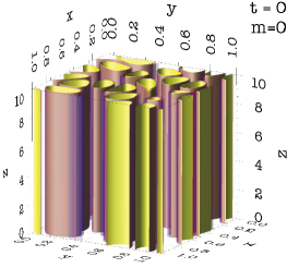
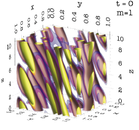
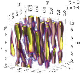
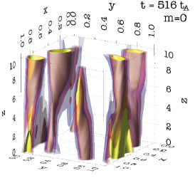
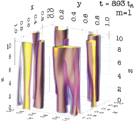
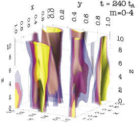
Figure 9.— Isosurfaces of the magnetic potential $\psi$ (in yellow and transparent red and blue colors) for the three-dimensional simulations with line-tied boundary conditions runs B, C and D, with respectively single parallel modes $m=0$, $m=1$ and all modes $m\in[0,4]$, and initial conditions with $b_{0}/B_{0}=10\%$. The elongated structure of $\psi$ along $z$ shows that in the asymptotic regime the fields relax into an equilibrium with a strong parallel m=0 mode not only for run B, that initially has only the mode m=0, but for all the initial conditions considered, including runs C that initially has only the parallel mode m=1 and run D that is started with many parallel modes. Snapshots times, left to right, are respectively $t=516\,\tau_{A}$, $893\,\tau_{A}$ and $240\,\tau_{A}$. The magnetic potential $\psi$ is defined in Section 2. The computational box has been rescaled for an improved visualization, but the axial length is ten times longer that the perpendicular cross section length.

4.3. Runs D: modes m=0–4

In this section we analyze numerical simulations (runs D) in which the initial magnetic field $\mathbf{b}$ includes all parallel modes $m\in[0,4]$, while large-scale perpendicular modes are set as in previous simulations with wavenumbers between 3 and 4 (Section 2.1, Equation [3]). The parallel zero mode is the strongest, with higher parallel modes having less energy. For all runs the fraction of magnetic energy in the parallel mode $m$, indicated with $\mathscr{E}_{m}$, is set in the initial magnetic field (Equation [3]) so that $\mathscr{E}_{m}/\mathscr{E}_{0}=(m+1)^{-2.6}$, corresponding to a progressively smaller energy for higher modes. Explicitly $\mathscr{E}_{m}/\mathscr{E}_{0}$ = 16.5%, 5.7%, 2.7%, 1.5% for $m\in[1,4]$. This specific choice of values is arbitrary, but the presence of multiple parallel modes of decreasing weight is chosen to represent the coronal field induced by photospheric motions in which multiple frequencies are present. Although to date there are no measurements of the spectrum of photospheric velocities, the presence of higher frequency modes with decreasingly smaller amplitudes is expected. Since smaller granules are expected to have faster convective timescales this is partially confirmed by the recent detection of mini-granular structures with their size distributed as a power law with an approximate Kolmogorov index $\sim-5/3$ and dominant on scales smaller than $600$ km (Abramenko et al., 2012).

As shown in Figure 7 (right panel) the dynamics are analogous to those of run B with only the parallel mode $m=0$ (cf. Figure 2). The dissipated energy decreases for lower values of $b_{0}/B_{0}$, but unlike runs B a small but discernible energy dissipation occurs also for very small ratios of $b_{0}/B_{0}$. Each run D dissipates a larger fraction of magnetic energy respect to the corresponding run B with same $b_{0}/B_{0}$ before reaching the asymptotic regime (cf. insets in Figures 7 and 2), because initially a fraction of the energy in runs D is in parallel modes higher than zero, and they will be dissipated during the decay so that the system can relax to equilibrium (dominated by the mode $m=0$ with variation length-scale $z_{\ell}\gtrsim L_{z}$).

Dynamics in physical space are also similar to those of run B, as shown in Figure 8 (bottom row) for $b_{0}/B_{0}=10\%$, with current sheets forming and dissipating energy thus leading to a relaxed field with larger magnetic islands through an inverse cascade. The evolution of the three-dimensional structure of the magnetic potential $\psi$, shown in Figure 9 (right column), is similar to those of runs B and C. The relaxed magnetic potential at $t=240\,\tau_{A}$ has a structure elongated along $z$, with a strong $m=0$ parallel mode similarly to runs B and C, even if its structure at time $t=0$ is considerably more complex due to the presence of multiple parallel scales ($m\in[0,4]$).

5. Conclusions and Discussion

Equilibria and dynamics of the magnetically confined regions of solar and stellar atmospheres have been investigated with a reduced MHD cartesian model to advance our understanding of the mechanism that powers the X-ray activity of the Sun, late-type main sequence stars, and more in general of stars with a magnetized corona and an outer convective envelope.

Since equilibria play a pivotal role in understanding the dynamics of this system, their structure has been analyzed in detail in Section 3. The mapping between the solutions of the 2D Euler equation $\mathbf{u}_{2D}(\mathbf{x},t)$ and reduced MHD equilibria $\mathbf{b}_{eq}(\mathbf{x}_{\perp},z)$ (Equation [10]: $t\rightarrow z$, $\mathbf{u}_{2D}\rightarrow\mathbf{b}_{eq}/B_{0}$) allows to formulate a heuristic quantitative analysis of the structure of the reduced MHD equilibria. The inverse cascade developed by the solutions of the Euler equation in time, corresponds to an asymmetric structure along $z$ of the reduced MHD equilibria, as pictorially summarized in Figure 1.

In similar fashion to 2D velocity vortices of scale $\ell$ that double their size in about one eddy turnover time $t_{\ell}\sim\ell/u_{\ell}$ (Equation [13]), a reduced MHD equilibrium with orthogonal magnetic field of intensity $b_{bd}$ at the bottom boundary $z=0$, and made of magnetic islands of scale $\ell$, will have progressively larger magnetic islands at larger $z$, doubling their transverse scale over the axial spatial distance

$$z_{\ell}\sim\frac{B_{0}}{b_{bd}}\,\ell.$$ (28)

This represents the parallel variation length-scale of the equilibrium solution, and measures quantitatively its asymmetry. An equilibrium is strongly asymmetric along $z$ if the variation scale is smaller than the loop length $z_{\ell}<L_{z}$, but if the variation scale is greater than approximately the loop length $z_{\ell}\gtrsim L_{z}$ then the equilibrium is quasi-invariant along $z$ (at the loop scale).

On the other hand in reduced MHD any spatial variation of the physical fields along $z$ is rapidly propagated away at the Alfvén speed $B_{0}$ (the fastest speed in the system) by the linear terms $\propto B_{0}\partial_{z}$ in Equations (1)-(2). Therefore the physical solutions cannot develop strongly asymmetric structures along $z$, as confirmed by boundary forced and decaying numerical simulations with line-tying boundary conditions and a strong guide field (e.g., Galsgaard & Nordlund, 1996; Dmitruk & Gómez, 1999; Rappazzo et al., 2008; Wilmot-Smith et al., 2011; Dahlburg et al., 2012). This implies that physical solutions are close to an equilibrium or not depending on the intensity of the orthogonal component of the magnetic field $b$, that regulates the value of the parallel equilibrium variation scale $z_{\ell}$ (28) for a given guide field of intensity $B_{0}$. Consequently the reduced MHD equilibria that can be accessed dynamically are those quasi-invariant along $z$ with an orthogonal magnetic field component $\mathbf{b}$ for which the parallel length-scale is greater than approximately the loop length $z_{\ell}\gtrsim L_{z}$.

The simulations reported by Rappazzo & Parker (2013), analyzed in detail in Section 4.1 (runs A–B), are in agreement with this picture. They considered initial magnetic fields $\mathbf{b_{0}}$ invariant along $z$ (i.e., only the parallel mode $m=0$ is present initially and $\partial j_{0}=0$), but with different intensities and non-vanishing Lorentz force for the perpendicular magnetic field, i.e., $\mathbf{b}_{0}\cdot\nabla j_{0}\neq 0$, and identified the magnetic field intensity threshold $b\sim\ell B_{0}/L_{z}$, corresponding to the critical variation scale $z_{\ell}\sim L_{z}$. Initial conditions with $b_{0}>\ell B_{0}/L_{z}$ ($z_{\ell}<L_{z}$) have dynamics increasingly similar to 2D MHD turbulence decay for larger values of $b_{0}$, with the orthogonal magnetic field forming current sheets and dissipating energy that decays as a power-law in time with $E\propto t^{-\alpha}$ ($\alpha\sim 1$ for $b_{0}/B_{0}=10\%$, Figure 2). As shown in Equation (18) in the 2D case the evolution of fields with different initial intensities is self-similar in time with $\mathbf{b}^{\prime}(t)=\mathbf{b}(t\cdot b^{\prime}_{0}/b_{0})\,b^{\prime}_{0}/b_{0}$, implying that they all decay with same power-law index and relax to asymptotic fields with intensities proportional to their initial value $b^{\prime}_{\infty}/b^{\prime}_{0}=b_{\infty}/b_{0}$. But in stark contrast with the 2D case the line-tied 3D simulations decay with progressively shallower power-laws (Figure 2) for weaker initial magnetic fields with smaller ratios $b_{0}/B_{0}$, relaxing to asymptotic equilibria for which the ratio $b_{\infty}/b_{0}$ is not independent from $b_{0}$. Instead $b_{\infty}\sim\ell B_{0}/L_{z}$, corresponding to a variation scale approximately equal to the loop length $z_{\ell}\sim L_{z}$ (as explained in Section 4.1 the orthogonal scale $\ell$ increases for stronger magnetic field because an inverse cascade of magnetic energy occurs). Furthermore initial magnetic fields with intensity below the threshold $b_{0}\lesssim\ell B_{0}/L_{z}$ ($z_{\ell}\gtrsim L_{z}$) show little dynamics with no significant decay nor current sheets formation and dissipation.

Therefore these simulations confirm numerically that the dynamically accessible equilibria are those quasi-invariant along $z$ (i.e., with a dominant $m=0$ mode) with magnetic field intensity smaller than the threshold $b\lesssim\ell B_{0}/L_{z}$, and corresponding parallel variation length-scale larger than approximately the loop length $z_{\ell}\gtrsim L_{z}$. The nature of this equilibria is radically different from the classic reduced MHD equilibria considered in plasma and solar physics in the framework of linear instabilities (kink, tearing, etc.), that typically are strictly invariant along $z$ ($\partial_{z}=0$) and in the reduced MHD framework have a vanishing orthogonal Lorenz force component with $\mathbf{b}\cdot\nabla j=0$. This condition is satisfied by very symmetric fields, e.g., a sheared field, or circular field lines (examples can be found in Parker, 1983; Longcope & Strauss, 1993, and references therein). But our initial magnetic fields (Section 2.1) have non-vanishing orthogonal Lorentz forces ($\mathbf{b}\cdot\nabla j\neq 0$), a property that stems from the complexity and disorder of photospheric motions. As shown in Figure 5 and 6 both terms in the equilibrium Equation (8) do not vanish as the system relaxes to equilibrium, with their rms $\sigma_{z}$ and $\sigma_{\perp}$ (Equation [20]) getting asymptotically equal, while the rms of their sum $\sigma_{eq}$ (Equation [21]) vanishes asymptotically as a power-law. Consequently the system does not relax to a classic linearly unstable equilibrium with $\partial_{z}j=0$ and $\mathbf{b}\cdot\nabla j=0$, as confirmed by a visual inspection of the orthogonal magnetic field $\mathbf{b}$ in Figure 4 (right column).

The simulations (runs B) have very different dynamics whether their initial parallel variation scales are larger or smaller than the critical length-scale $z_{\ell}\sim L_{z}$. For $z_{\ell}<L_{z}$, with $b>\ell B_{0}/L_{z}$, the initial magnetic field is very far from the corresponding equilibrium, as this is too asymmetric along $z$ and is therefore dynamically inaccessible. The only way for the out-of-equilibrium field to reach an equilibrium is therefore to decay to a lower energy configuration with smaller $b$ until the critical length scale $z_{\ell}\sim L_{z}$ is reached, and this necessarily implies the formation of current sheets and dissipation through nonlinear dynamics (a magnetically dominated nonlinear MHD turbulent cascade analyzed in depth in Rappazzo & Velli, 2011). On the contrary initial magnetic fields with $z_{\ell}\gtrsim L_{z}$, for which $b\lesssim\ell B_{0}/L_{z}$, are very close to the corresponding equilibrium because they are both elongated along $z$. Thus the field simply readjusts to the close equilibrium with no significant nonlinear dynamics, current sheet formation nor dissipation, as shown in Figures 2–4 and particularly in Figures 5 and 6. Strictly speaking also in this case a very small energy dissipation occurs, but it is negligible, does not involve the formation of significantly stronger currents, and additionally nonlinearities are diminished in close proximity to equilibrium.

The quasi-static evolution of the magnetic field is then restricted only to field intensities smaller than approximately $b\lesssim\ell B_{0}/L_{z}$, while stronger fields are necessarily out-of-equilibrium and develop turbulent dynamics with subsequent current sheet formation and energy dissipation.

Consequently two distinct stages can be identified in the dynamics of an initially uniform and strong axial magnetic field $B_{0}\mathbf{\hat{e}}_{z}$ shuffled at its footpoints by a constant or low frequency photospheric velocity $\mathbf{u}_{ph}$ (see Section 3.1 for a discussion on forcing frequencies). To mimic the solenoidal component of the photospheric horizontal velocity (the irrotational component cannot twist the field lines), the incompressible velocity at the boundary $\mathbf{u}_{ph}$ is made up of distorted vortices (see Rappazzo et al., 2008, for a specific example) with $\mathbf{u}_{ph}\cdot\nabla\omega_{ph}\neq 0$, given the general complexity and disorder of photospheric motions. At first photospheric motions generate an orthogonal coronal magnetic field component that grows linearly in time and is a mapping of the photospheric velocity, i.e., $\mathbf{b}=\mathbf{u}_{ph}\,t/\tau_{A}$ (Equation [16]). Until its intensity remains below the threshold $b\sim\ell B_{0}/L_{z}$ the field is essentially in equilibrium and nonlinearities do not develop, leading to its linear growth in time. In fact neglecting nonlinear terms in the reduced MHD equations, the linear growth follows from the remaining linear terms (Equation [15]) and boundary conditions. When the magnetic field intensity crosses the threshold the variation length-scale of the corresponding equilibrium becomes smaller than the loop length $z_{\ell}\lesssim L_{z}$. The structure of the equilibrium becomes then too asymmetric along $z$, while the dynamically induced magnetic field (Equation [16]) is quasi-invariant along $z$. The magnetic field is then too distant from its corresponding equilibrium that cannot be accessed dynamically unless the field intensity decreases. The Lorentz force components that were in equilibrium during the quasi-static stage now cannot reach a balance with each other, the magnetic field is therefore in non-equilibrium and nonlinear dynamics develop.

Parker (1988) had conjectured a two-stage process to account for the inferred Poynting flux in active regions, estimated by Withbroe & Noyes (1977) at about $S_{z}\sim 10^{7}$ erg cm^-2 s^-1. In fact if current sheet formation and energy dissipation would be effective at an earlier stage, with too weak magnetic fields, then the Poynting flux would be too small to sustain the X-ray activity of active regions. Reverting now to conventional units, the time and space averaged Poynting flux is given by $\langle S_{z}\rangle\sim S/\ell^{2}\sim\rho v_{A,\parallel}\,u_{ph}\,v_{A,\perp}$ (see Section 2.2, density $\rho$ and Alfvén velocities are introduced from dimensional calculations), where $v_{A,\parallel}=B_{0}/\sqrt{4\pi\rho}$ and $v_{A,\perp}=b/\sqrt{4\pi\rho}$ are the Alfvén velocities associated respectively to the guide field $B_{0}$ and the orthogonal magnetic field component $\mathbf{b}$. Introducing the threshold magnetic field intensity $b\sim\ell B_{0}/L_{z}$ (or the associated Alfvén velocity) we obtain for the Poynting flux:

$$\langle S_{z}\rangle\sim\rho\,v^{2}_{A,\parallel}u_{ph}\frac{\ell}{L_{z}}=\frac{B_{0}^{2}u_{ph}\ell}{4\pi L_{z}}.$$ (29)

This coincides with the strong guide field regime of the scaling relation obtained by Rappazzo et al. (2008) (Equation [68] with $\alpha\gg 1$) for boundary forced simulations, that yields for typical solar active region loops an energy flux $\sim 1.6\times 10^{6}$ erg cm^-2 s^-1, in the lower range of the constraint inferred by Withbroe & Noyes (1977). But recent fully compressible MHD simulations with similar setup, that include the integration of an energy equation with thermal conduction and energy losses provided by optically thin radiation, and in addition have density stratification (with strong gradients from the chromosphere to the corona), exhibit Poynting fluxes of the order of $\sim 10^{7}$ erg cm^-2 s^-1, and most importantly an X-ray emission that matches the physical properties of the observed radiation (Dahlburg et al., 2015, submitted).

Additionally numerical simulations with initial magnetic fields not invariant along $z$ have been carried out (runs C and D). Higher parallel modes can be present for both the Sun and other active stars of interest. They can be generated by the nonlinear dynamics even when photospheric motions have a low frequency, or they can be directly excited by photospheric motions in long loops, that on some stars have observationally inferred lengths of the order of several stellar radii (Favata et al., 2005; Getman et al., 2008; Peterson et al., 2010).

Runs C include only the parallel mode $m=1$, while for runs D all modes $m\in[0,4]$ are present. As in previously discussed runs B the initial magnetic field $\mathbf{b}_{0}$ is not in equilibrium, now with both terms in the equilibrium Equation (8) non-vanishing ($\mathbf{b}_{0}\cdot\nabla j_{0}\neq 0$ and $\partial_{z}j_{0}\neq 0$). Remarkably these initial conditions decay to equilibria with structures similar to those of runs B (whose initial magnetic fields included only the mode $m=0$), as shown in Figure 9. Independently from the structure of the initial magnetic field, and from the specific modes that it includes, the final equilibrium is always quasi-invariant along $z$ with parallel variation length-scale larger than approximately the loop length $z_{\ell}\gtrsim L_{z}$. Its structure is elongated along the axial direction, a strong $m=0$ parallel mode is present, and the magnetic field intensity is smaller than the threshold value $b\lesssim\ell B_{0}/L_{z}$. This further confirms the analysis of the equilibria performed in Section 3.1, i.e., that the reduced MHD equilibria dynamically accessible in a line-tied configuration are elongated along the axial direction with a dominant $m=0$ parallel mode. It also implies that nonlinear dynamics can transfer energy from higher parallel modes to the mode $m=0$ even when this is not initially present (runs C), a process that can be of interest also in periodic turbulence (Alexakis, 2011; Schekochihin et al., 2012), and has been conjectured to play a role in the dynamics that lead to the acceleration of the solar wind (Dmitruk et al., 2001).

In contrast to runs B, with initial conditions invariant along $z$, that decay only for magnetic field intensities above the threshold $b\sim\ell B_{0}/L_{z}$, in runs C a decay is always observed independently from the intensity of the initial magnetic field (Figure 7). Since the accessible equilibria are quasi-invariant along $z$ and the initial magnetic field of runs C does not contain the $m=0$ mode but only the $m=1$ mode, then it always decays. The asymptotic stage is reached when the mode $m=0$ has been generated and excess energy in higher modes dissipated. The intensity of the relaxed magnetic field depends on the ability of nonlinear dynamics to transfer energy among higher parallel modes and from these to the $m=0$ mode, but the longer decay timescales for lower values of $b_{0}/B_{0}$ are consistent with a decrease of the strength of nonlinear interactions (e.g., the eddy turnover time decreases ad $t_{\ell}\sim 2\ell/b_{0}$, see Section 4.2). The longer nonlinear timescales render the effect of a high-frequency resonant photospheric forcing similar in many aspects to that of a constant photospheric velocity (see Section 4.2 for a more complete discussion). In fact if a photospheric velocity with a higher resonant frequency $\nu_{n}=n\nu_{A}/2$ with $n\geq 1$ is applied at the boundary, nonlinear terms can be neglected initially because for low values of the magnetic field intensity $b$ the decay timescales are much longer than the linear growth of the magnetic field. A statistical steady state will finally be obtained when the energy flux injected in the system at the boundary by photospheric motions is balanced by a similar energy flux from the large toward the small scales (to form current sheets), in similar fashion to the constant velocity case (Rappazzo et al., 2007).

When initial conditions include higher parallel modes $m\in[0,4]$ and the $m=0$ mode has the largest amplitude (runs D, Section 4.3) the dynamics are very similar to runs B with only the $m=0$ mode in the initial conditions (cf. Figures 2 and 7). The excess energy in higher parallel modes is either dissipated or transferred to the $m=0$ mode and the relaxed fields have structures similar to runs B and C (Figure 9).

The parallel variation scale $z_{\ell}\sim\ell B_{0}/b$ introduced here (Equation [28]) can be interpreted as a critical length or twist. In fact given the magnetic field intensity $b$, significant nonlinear dynamics will develop only if the loop length is longer than the variation scale $L_{z}\gtrsim z_{\ell}$. On the other hand, fixed the loop length $L_{z}$ nonlinear dynamics will develop only if the variation scale is smaller than the loop length $z_{\ell}\lesssim L_{z}$, or equivalently if the field intensity is larger than the threshold $b\gtrsim\ell B_{0}/L_{z}$, that corresponds to an average twist larger than $\langle\Phi\rangle\sim L_{z}b/(\ell B_{0})\gtrsim\pi/3$ (this is only an estimate, since the orthogonal field does not have cylindrical symmetry $b\neq b(r)$, the twist should be computed numerically for sample field lines).

The concept of a critical length or twist has been developed in the study of several linear instabilities in coronal loops with line-tied boundary conditions, including kink and tearing instabilities (Raadu, 1972; Hood & Priest, 1979, 1981; Einaudi & van Hoven, 1981, 1983; Velli & Hood, 1989; Velli et al., 1990; Foote & Craig, 1990; Lionello et al., 1998; Huang & Zweibel, 2009; Huang et al., 2010). It is found that the system is linearly unstable for a fixed magnetic field intensity only if the loop length is larger than a critical value (for kink and other instabilities a critical twist can be used equivalently).

It is important to remark that although it is useful to regard the parallel variation scale $z_{\ell}$ (Equation [28]) as a critical length, and that an average critical twist can be defined, the dynamics that they help describe are not linear instabilities. In the configurations of interest to this paper the critical length or twist distinguish two different dynamic regimes in which respectively for small field intensities $b$ nonlinear dynamics are suppressed and the evolution can be regarded as quasi-static, while for stronger intensities nonlinear dynamics develop. Of course the boundary between these two regimes is not sharp, but gradually as $b$ is increased the “2D” Lorentz force $\mathbf{b}\cdot\nabla\mathbf{b}$ cannot be balanced by the axial field line tension $B_{0}\partial_{z}\mathbf{b}$, leading the system out of equilibrium. In particular all the 3D line-tied magnetic fields that we have considered lack the symmetries of linearly unstable configurations, and for all of them the orthogonal component of the magnetic field is not symmetric and its 2D Lorentz force component (for which $\mathbf{b}\cdot\nabla j\neq 0$) does not vanish at all times, from the initial condition to the relaxed asymptotic stage, as can be seen in Figures 4-6, 8 and 9.

The reason for which the equilibria with $z_{\ell}\gtrsim L_{z}$ are not linearly unstable is that they are close to each other. Therefore adding a perturbation to the magnetic field simply changes slightly the corresponding equilibrium to which the field readjusts. For instance the initial condition of run B with $b_{0}/B_{0}=2\%$ is not exactly an equilibrium (since $\partial_{z}j_{0}=0$ and $\mathbf{b}_{0}\cdot\nabla j_{0}\neq 0$), therefore it can be regarded as an equilibrium to which has been added a small perturbation. But as shown particularly well in Figure 8 (bottom panel) no instability of sort is detected, rather the field undergoes a slight readjustment. Clearly for a non-vanishing orthogonal magnetic field $\mathbf{b}$ in equilibrium, with a progressively smaller 2D Lorentz force component for which $\mathbf{b}\cdot\nabla j\rightarrow 0$ (with $b\neq 0$), the field approaches a symmetric configuration that can be linearly unstable, since from the equilibrium Equation (8) also $\partial_{z}j\rightarrow 0$ in this limit. But as previously discussed the configurations of interest here are those with non-vanishing orthogonal 2D Lorentz force component $\mathbf{b}\cdot\nabla j\neq 0$.

The relaxation of coronal magnetic fields has often been studied subsequently to a linear instability, mostly kink modes. Particularly for the cases that have a strong axial magnetic field the structure of the lower energy relaxed field appears elongated along $z$ (Mikic et al., 1990; Longcope & Strauss, 1994; Baty & Heyvaerts, 1996; Velli et al., 1997; Lionello et al., 1998; Baty, 2000; Gerrard et al., 2002; Browning et al., 2008; Hood et al., 2009). Early boundary forced simulations have been performed by Ng & Bhattacharjee (1998), with similar setup as those of Rappazzo et al. (2008). But due to their low resolution they misinterpret as an instability the dynamics that develop as the threshold $b\sim\ell B_{0}/L_{z}$ is crossed, when the system gradually transitions from quasi-static evolution to turbulent dynamics. From the simulations (runs B) and the equilibria analysis it is clear that the forces that are approximatively in balance below the threshold become gradually unbalanced for larger magnetic field intensities, leading to the development of nonlinear dynamics with no intermediate instability as would occur for instance with a kink mode, where the nonlinear stage would follow the linear instability. The non-vanishing 2D Lorentz force term $\mathbf{b}\cdot\nabla\mathbf{b}$ (for which $\mathbf{b}\cdot\nabla j\neq 0$), that in the 2D case (run A) sets the system out-of-equilibrium and develops turbulent nonlinear dynamics, can be balanced in the 3D line-tied runs B by the axial field line tension term $B_{0}\partial_{z}\mathbf{b}$ for field intensities below the threshold $b\lesssim\ell B_{0}/L_{z}$. For larger magnetic field intensities the 2D Lorentz force term is stronger than its axial component, hence the dynamics develop progressively more akin to the 2D case. Ultimately a force balance cannot be reached because the corresponding equilibrium is too asymmetric along $z$ and therefore dynamically inaccessible, so that for larger intensities $b$ a larger fraction of energy must be necessarily dissipated for the system to be able to relax and access a new equilibrium.

This two-stage process then provides a fully self-consistent alternative to coronal heating models based on instabilities. For instance, since resistive instabilities are slow for macroscopically thick magnetic shears, Dahlburg et al. (2005, 2009) obtain a shear intensity threshold for dissipation supposing that nanoflares would occur when photospheric motions shear the magnetic field beyond a certain angle, when a secondary ideal instability (triggered by the slow primary resistive instability) can develop thus accelerating the dynamics. On the other hand, as discussed in this paper, as photospheric motions disorderly twist the field lines, once the magnetic field intensity is higher than the threshold $b\gtrsim\ell B_{0}/L_{z}$ magnetically dominated turbulent dynamics develop, forming current sheets that thin down to the dissipative scales on fast Alfvén time-scales (Rappazzo & Parker, 2013), while triggering the “ideal” tearing instability (see Introduction; Pucci & Velli, 2014; Landi et al., 2015; Tenerani et al., 2015), and leading to dynamics similar to so-called plasmoid instability (Bulanov et al., 1978; Biskamp, 1986; Loureiro et al., 2007; Lapenta, 2008; Bhattacharjee et al., 2009).

Finally, these simulations of decaying magnetic fields show that, beyond the intensity threshold [Equation (28)], current sheets form on fast ideal timescales because of the nonlinear dynamics that develop. This is in stark contrast with the frequent hypothesis of quasi-static evolution of the coronal magnetic field subject to footpoint shuffling, that should continuously relax to a nearby equilibrium without forming current sheets (e.g., van Ballegooijen, 1985). In the quasi-static scenario the corona could be heated by the uniformly distributed small-scale current sheets created by the shredding of the coronal magnetic field after many successive random walk steps of its field lines footpoints  (van Ballegooijen, 1986). But this mechanism would lead to current sheet formation on timescale longer than photospheric convection (several random walk steps would be required). While the relaxation simulations presented in this paper and in Rappazzo & Parker (2013) show that current sheets form on ideal Alfvén timescales (much faster than convective timescales), with the footpoints fixed at the photospheric plates where no motions are in place (and therefore no footpoint random walk occurs).

References

- Abramenko et al. (2012) Abramenko, V. I., Yurchyshyn, V. B., Goode, P. R., Kitiashvili, I. N., & Kosovichev, A. G. 2012, ApJ, 756, L27
- Alexakis (2011) Alexakis, A. 2011, Phys. Rev. E, 84, 056330
- Aluie & Eyink (2010) Aluie, H., & Eyink, G. L. 2010, Physical Review Letters, 104, 081101
- Antiochos (1987) Antiochos, S. K. 1987, ApJ, 312, 886
- Batchelor (1969) Batchelor, G. K. 1969, Physics of Fluids, 12, 233
- Baty (2000) Baty, H. 2000, A&A, 360, 345
- Baty & Heyvaerts (1996) Baty, H., & Heyvaerts, J. 1996, A&A, 308, 935
- Beeck et al. (2013) Beeck, B., Cameron, R. H., Reiners, A., & Schüssler, M. 2013, A&A, 558, A48
- Belmonte et al. (1999) Belmonte, A., Goldburg, W. I., Kellay, H., et al. 1999, Physics of Fluids, 11, 1196
- Beresnyak (2013) Beresnyak, A. 2013, ArXiv e-prints, arXiv:1301.7424
- Bertozzi & Constantin (1993) Bertozzi, A. L., & Constantin, P. 1993, Communications in Mathematical Physics, 152, 19
- Bhattacharjee et al. (2009) Bhattacharjee, A., Huang, Y.-M., Yang, H., & Rogers, B. 2009, Physics of Plasmas, 16, 112102
- Birn et al. (2001) Birn, J., Drake, J. F., Shay, M. A., et al. 2001, J. Geophys. Res., 106, 3715
- Biskamp (1986) Biskamp, D. 1986, Physics of Fluids, 29, 1520
- Biskamp (2003) Biskamp, D. 2003, Magnetohydrodynamic Turbulence (Cambridge: Cambridge University Press)
- Boffetta & Ecke (2012) Boffetta, G., & Ecke, R. E. 2012, Annual Review of Fluid Mechanics, 44, 427
- Bogoyavlenskij (2000) Bogoyavlenskij, O. I. 2000, Physical Review Letters, 84, 1914
- Brachet et al. (2013) Brachet, M. E., Bustamante, M. D., Krstulovic, G., et al. 2013, Phys. Rev. E, 87, 013110
- Browning et al. (2008) Browning, P. K., Gerrard, C., Hood, A. W., Kevis, R., & van der Linden, R. A. M. 2008, A&A, 485, 837
- Buchlin & Velli (2007) Buchlin, E., & Velli, M. 2007, ApJ, 662, 701
- Bulanov et al. (1978) Bulanov, S. V., Syrovatskii, S. I., & Sakai, J. 1978, ZhETF Pisma Redaktsiiu, 28, 193
- Canuto et al. (2006) Canuto, C., Hussaini, M. Y., Quarteroni, A., & Zang, T. A. 2006, Spectral Methods (Berlin: Springer-Verlag), doi:10.1007/978-3-540-30726-6
- Chemin (1993) Chemin, J.-Y. 1993, Annales scientifiques de l’École Normale Supérieure, 26, 517
- Chiuderi & Velli (2015) Chiuderi, C., & Velli, M. 2015, Basics of Plasma Astrophysics (Berlin: Springer-Verlag)
- Cowley et al. (1997) Cowley, S. C., Longcope, D. W., & Sudan, R. N. 1997, Phys. Rep., 283, 227
- Dahlburg et al. (2012) Dahlburg, R. B., Einaudi, G., Rappazzo, A. F., & Velli, M. 2012, A&A, 544, L20
- Dahlburg et al. (2015, submitted) Dahlburg, R. B., Einaudi, G., Taylor, B., et al. 2015, submitted, ApJ
- Dahlburg et al. (2005) Dahlburg, R. B., Klimchuk, J. A., & Antiochos, S. K. 2005, ApJ, 622, 1191
- Dahlburg et al. (2009) Dahlburg, R. B., Liu, J.-H., Klimchuk, J. A., & Nigro, G. 2009, ApJ, 704, 1059
- De Pontieu et al. (2007) De Pontieu, B., McIntosh, S. W., Carlsson, M., et al. 2007, Science, 318, 1574
- Dmitruk & Gómez (1997) Dmitruk, P., & Gómez, D. O. 1997, ApJ, 484, L83
- Dmitruk & Gómez (1999) —. 1999, ApJ, 527, L63
- Dmitruk et al. (1998) Dmitruk, P., Gómez, D. O., & DeLuca, E. E. 1998, ApJ, 505, 974
- Dmitruk et al. (2003) Dmitruk, P., Gómez, D. O., & Matthaeus, W. H. 2003, Physics of Plasmas, 10, 3584
- Dmitruk et al. (2001) Dmitruk, P., Matthaeus, W. H., Milano, L. J., & Oughton, S. 2001, Physics of Plasmas, 8, 2377
- Donati & Landstreet (2009) Donati, J.-F., & Landstreet, J. D. 2009, ARA&A, 47, 333
- Dryden (1943) Dryden, H. L. 1943, Quarterly of Applied Mathematics, 1, 7
- Einaudi & van Hoven (1981) Einaudi, G., & van Hoven, G. 1981, Physics of Fluids, 24, 1092
- Einaudi & van Hoven (1983) —. 1983, Sol. Phys., 88, 163
- Einaudi & Velli (1999) Einaudi, G., & Velli, M. 1999, Physics of Plasmas, 6, 4146
- Einaudi et al. (1996) Einaudi, G., Velli, M., Politano, H., & Pouquet, A. 1996, ApJ, 457, L113
- Euler (1761) Euler, L. 1761, Novi Commentarii Acad. Sci. Petropolitanae, 6, 271
- Favata et al. (2005) Favata, F., Flaccomio, E., Reale, F., et al. 2005, ApJS, 160, 469
- Foote & Craig (1990) Foote, B. J., & Craig, I. J. D. 1990, ApJ, 350, 437
- Frisch & Sulem (1984) Frisch, U., & Sulem, P. L. 1984, Physics of Fluids, 27, 1921
- Galsgaard & Nordlund (1996) Galsgaard, K., & Nordlund, Å. 1996, J. Geophys. Res., 101, 13445
- Galtier et al. (1997) Galtier, S., Politano, H., & Pouquet, A. 1997, Physical Review Letters, 79, 2807
- Georgoulis et al. (1998) Georgoulis, M. K., Velli, M., & Einaudi, G. 1998, ApJ, 497, 957
- Gerrard et al. (2002) Gerrard, C. L., Arber, T. D., & Hood, A. W. 2002, A&A, 387, 687
- Getman et al. (2008) Getman, K. V., Feigelson, E. D., Micela, G., et al. 2008, ApJ, 688, 437
- Gharib & Derango (1989) Gharib, M., & Derango, P. 1989, Physica D Nonlinear Phenomena, 37, 406
- Gold (1964) Gold, T. 1964, NASA Special Publication, 50, 389
- Gold & Hoyle (1960) Gold, T., & Hoyle, F. 1960, MNRAS, 120, 89
- Greffier et al. (2002) Greffier, O., Amarouchene, Y., & Kellay, H. 2002, Physical Review Letters, 88, 194101
- Güdel (2004) Güdel, M. 2004, A&A Rev., 12, 71
- Güdel (2009) Güdel, M. 2009, in Lecture Notes in Physics, Berlin Springer Verlag, Vol. 778, Turbulence in Space Plasmas, ed. P. Cargill & L. Vlahos, 269
- Hasegawa (1985) Hasegawa, A. 1985, Advances in Physics, 34, 1
- Hendrix & van Hoven (1996) Hendrix, D. L., & van Hoven, G. 1996, ApJ, 467, 887
- Hood et al. (2009) Hood, A. W., Browning, P. K., & van der Linden, R. A. M. 2009, A&A, 506, 913
- Hood & Priest (1979) Hood, A. W., & Priest, E. R. 1979, Sol. Phys., 64, 303
- Hood & Priest (1981) —. 1981, Geophysical and Astrophysical Fluid Dynamics, 17, 297
- Hossain et al. (1983) Hossain, M., Matthaeus, W. H., & Montgomery, D. 1983, Journal of Plasma Physics, 30, 479
- Hossain et al. (1995) Hossain, M., Gray, P. C., Pontius, Jr., D. H., Matthaeus, W. H., & Oughton, S. 1995, Physics of Fluids, 7, 2886
- Huang & Bhattacharjee (2010) Huang, Y.-M., & Bhattacharjee, A. 2010, Physics of Plasmas, 17, 062104
- Huang et al. (2010) Huang, Y.-M., Bhattacharjee, A., & Zweibel, E. G. 2010, Physics of Plasmas, 17, 055707
- Huang & Zweibel (2009) Huang, Y.-M., & Zweibel, E. G. 2009, Physics of Plasmas, 16, 042102
- Ionson (1985) Ionson, J. A. 1985, A&A, 146, 199
- Kadomtsev & Pogutse (1974) Kadomtsev, B. B., & Pogutse, O. P. 1974, Soviet Journal of Experimental and Theoretical Physics, 38, 283
- Kaneda et al. (2003) Kaneda, Y., Ishihara, T., Yokokawa, M., Itakura, K., & Uno, A. 2003, Physics of Fluids, 15, L21
- Klimchuk (2006) Klimchuk, J. A. 2006, Sol. Phys., 234, 41
- Kolmogorov (1941) Kolmogorov, A. 1941, Akademiia Nauk SSSR Doklady, 30, 301
- Kraichnan (1967) Kraichnan, R. H. 1967, Physics of Fluids, 10, 1417
- Kraichnan & Montgomery (1980) Kraichnan, R. H., & Montgomery, D. 1980, Reports on Progress in Physics, 43, 547
- Landi et al. (2015) Landi, S., Del Zanna, L., Papini, E., Pucci, F., & Velli, M. 2015, ApJ, 806, 131
- Lapenta (2008) Lapenta, G. 2008, Physical Review Letters, 100, 235001
- Lazarian & Vishniac (1999) Lazarian, A., & Vishniac, E. T. 1999, ApJ, 517, 700
- Lionello et al. (1998) Lionello, R., Velli, M., Einaudi, G., & Mikić, Z. 1998, ApJ, 494, 840
- Longcope & Strauss (1993) Longcope, D. W., & Strauss, H. R. 1993, Physics of Fluids B, 5, 2858
- Longcope & Strauss (1994) —. 1994, ApJ, 426, 742
- Loureiro et al. (2007) Loureiro, N. F., Schekochihin, A. A., & Cowley, S. C. 2007, Physics of Plasmas, 14, 100703
- Loureiro et al. (2009) Loureiro, N. F., Uzdensky, D. A., Schekochihin, A. A., Cowley, S. C., & Yousef, T. A. 2009, MNRAS, 399, L146
- Low (2013) Low, B. C. 2013, ApJ, 768, 7
- Low (2015) —. 2015, Science China Physics, Mechanics, and Astronomy, 58, 2
- Ludwig et al. (2002) Ludwig, H.-G., Allard, F., & Hauschildt, P. H. 2002, A&A, 395, 99
- Majda & Bertozzi (2001) Majda, A. J., & Bertozzi, A. L. 2001, Vorticity and Incompressible Flow (Cambridge: Cambridge University Press)
- Martin et al. (2012) Martin, S. F., Panasenco, O., Berger, M. A., et al. 2012, in Astronomical Society of the Pacific Conference Series, Vol. 463, Second ATST-EAST Meeting: Magnetic Fields from the Photosphere to the Corona., ed. T. R. Rimmele, A. Tritschler, F. Wöger, M. Collados Vera, H. Socas-Navarro, R. Schlichenmaier, M. Carlsson, T. Berger, A. Cadavid, P. R. Gilbert, P. R. Goode, & M. Knölker, 157
- Matthaeus & Montgomery (1980) Matthaeus, W. H., & Montgomery, D. 1980, Annals of the New York Academy of Sciences, 357, 203
- Matthaeus et al. (1991) Matthaeus, W. H., Stribling, W. T., Martinez, D., Oughton, S., & Montgomery, D. 1991, Physical Review Letters, 66, 2731
- Mikic et al. (1990) Mikic, Z., Schnack, D. D., & van Hoven, G. 1990, ApJ, 361, 690
- Milano et al. (1997) Milano, L. J., Gómez, D. O., & Martens, P. C. H. 1997, ApJ, 490, 442
- Mininni & Pouquet (2013) Mininni, P. D., & Pouquet, A. 2013, Phys. Rev. E, 87, 033002
- Montgomery (1982) Montgomery, D. 1982, Physica Scripta Volume T, 2, 83
- Ng & Bhattacharjee (1998) Ng, C. S., & Bhattacharjee, A. 1998, Physics of Plasmas, 5, 4028
- Nigro et al. (2008) Nigro, G., Malara, F., & Veltri, P. 2008, ApJ, 685, 606
- Parker (1957) Parker, E. N. 1957, J. Geophys. Res., 62, 509
- Parker (1972) —. 1972, ApJ, 174, 499
- Parker (1979) —. 1979, Cosmical magnetic fields: Their origin and their activity (New York: Oxford University Press)
- Parker (1983) —. 1983, ApJ, 264, 635
- Parker (1988) —. 1988, ApJ, 330, 474
- Parker (1994) —. 1994, Spontaneous current sheets in magnetic fields (New York: Oxford University Press)
- Parker (2000) —. 2000, Physical Review Letters, 85, 4405
- Parker (2012) —. 2012, Plasma Physics and Controlled Fusion, 54, 124028
- Pearson et al. (2002) Pearson, B. R., Krogstad, P.-Å., & van de Water, W. 2002, Physics of Fluids, 14, 1288
- Peter et al. (2013) Peter, H., Bingert, S., Klimchuk, J. A., et al. 2013, A&A, 556, A104
- Peterson et al. (2010) Peterson, W. M., Mutel, R. L., Güdel, M., & Goss, W. M. 2010, Nature, 463, 207
- Priest (2014) Priest, E. 2014, Magnetohydrodynamics of the Sun (Cambridge: Cambridge University Press)
- Pucci & Velli (2014) Pucci, F., & Velli, M. 2014, ApJ, 780, L19
- Raadu (1972) Raadu, M. A. 1972, Sol. Phys., 22, 425
- Rappazzo (2006) Rappazzo, A. F. 2006, PhD thesis, Università di Pisa
- Rappazzo & Parker (2013) Rappazzo, A. F., & Parker, E. N. 2013, ApJ, 773, L2
- Rappazzo & Velli (2011) Rappazzo, A. F., & Velli, M. 2011, Phys. Rev. E, 83, 065401
- Rappazzo et al. (2007) Rappazzo, A. F., Velli, M., Einaudi, G., & Dahlburg, R. B. 2007, ApJ, 657, L47
- Rappazzo et al. (2008) —. 2008, ApJ, 677, 1348
- Reale (2014) Reale, F. 2014, Living Reviews in Solar Physics, 11, 4
- Reiners (2012) Reiners, A. 2012, Living Reviews in Solar Physics, 9, 1
- Rivera et al. (2003) Rivera, M. K., Daniel, W. B., Chen, S. Y., & Ecke, R. E. 2003, Physical Review Letters, 90, 104502
- Rose & Sulem (1978) Rose, H. A., & Sulem, P. L. 1978, Journal de Physique France, 39, 441
- Rosner & Knobloch (1982) Rosner, R., & Knobloch, E. 1982, ApJ, 262, 349
- Schekochihin et al. (2012) Schekochihin, A. A., Nazarenko, S. V., & Yousef, T. A. 2012, Phys. Rev. E, 85, 036406
- Shay et al. (1999) Shay, M. A., Drake, J. F., Rogers, B. N., & Denton, R. E. 1999, Geophys. Res. Lett., 26, 2163
- Shibata & Magara (2011) Shibata, K., & Magara, T. 2011, Living Reviews in Solar Physics, 8, 6
- Sommeria (1986) Sommeria, J. 1986, Journal of Fluid Mechanics, 170, 139
- Sreenivasan (1984) Sreenivasan, K. R. 1984, Physics of Fluids, 27, 1048
- Sreenivasan (1998) —. 1998, Physics of Fluids, 10, 528
- Strauss (1976) Strauss, H. R. 1976, Physics of Fluids, 19, 134
- Sturrock & Uchida (1981) Sturrock, P. A., & Uchida, Y. 1981, ApJ, 246, 331
- Sweet (1958) Sweet, P. A. 1958, in IAU Symposium, Vol. 6, Electromagnetic Phenomena in Cosmical Physics, ed. B. Lehnert, 123
- Tabeling (2002) Tabeling, P. 2002, Phys. Rep., 362, 1
- Taylor (1935) Taylor, G. I. 1935, Royal Society of London Proceedings Series A, 151, 421
- Taylor (1986) Taylor, J. B. 1986, Reviews of Modern Physics, 58, 741
- Tenerani et al. (2015) Tenerani, A., Rappazzo, A. F., Velli, M., & Pucci, F. 2015, ApJ, 801, 145
- Uzdensky et al. (2010) Uzdensky, D. A., Loureiro, N. F., & Schekochihin, A. A. 2010, Physical Review Letters, 105, 235002
- van Ballegooijen (1985) van Ballegooijen, A. A. 1985, ApJ, 298, 421
- van Ballegooijen (1986) —. 1986, ApJ, 311, 1001
- Velli & Hood (1989) Velli, M., & Hood, A. W. 1989, Sol. Phys., 119, 107
- Velli et al. (1990) Velli, M., Hood, A. W., & Einaudi, G. 1990, ApJ, 350, 428
- Velli et al. (1997) Velli, M., Lionello, R., & Einaudi, G. 1997, Sol. Phys., 172, 257
- Wan et al. (2009) Wan, M., Oughton, S., Servidio, S., & Matthaeus, W. H. 2009, Physics of Plasmas, 16, 080703
- Wilmot-Smith et al. (2009) Wilmot-Smith, A. L., Hornig, G., & Pontin, D. I. 2009, ApJ, 696, 1339
- Wilmot-Smith et al. (2011) Wilmot-Smith, A. L., Pontin, D. I., Yeates, A. R., & Hornig, G. 2011, A&A, 536, A67
- Withbroe & Noyes (1977) Withbroe, G. L., & Noyes, R. W. 1977, ARA&A, 15, 363
- Zank & Matthaeus (1992) Zank, G. P., & Matthaeus, W. H. 1992, Journal of Plasma Physics, 48, 85