Shrinkage degree in $L_{2}$-re-scale boosting for regression

Abstract

Re-scale boosting (RBoosting) is a variant of boosting which can essentially improve the generalization performance of boosting learning. The key feature of RBoosting lies in introducing a shrinkage degree to re-scale the ensemble estimate in each gradient-descent step. Thus, the shrinkage degree determines the performance of RBoosting. The aim of this paper is to develop a concrete analysis concerning how to determine the shrinkage degree in $L_{2}$-RBoosting. We propose two feasible ways to select the shrinkage degree. The first one is to parameterize the shrinkage degree and the other one is to develope a data-driven approach of it. After rigorously analyzing the importance of the shrinkage degree in $L_{2}$-RBoosting learning, we compare the pros and cons of the proposed methods. We find that although these approaches can reach the same learning rates, the structure of the final estimate of the parameterized approach is better, which sometimes yields a better generalization capability when the number of sample is finite. With this, we recommend to parameterize the shrinkage degree of $L_{2}$-RBoosting. To this end, we present an adaptive parameter-selection strategy for shrinkage degree and verify its feasibility through both theoretical analysis and numerical verification. The obtained results enhance the understanding of RBoosting and further give guidance on how to use $L_{2}$-RBoosting for regression tasks.

I Introduction

Boosting is a learning system which combines many parsimonious models to produce a model with prominent predictive performance. The underlying intuition is that combines many rough rules of thumb can yield a good composite learner. From the statistical viewpoint, boosting can be viewed as a form of functional gradient decent [1]. It connects various boosting algorithms to optimization problems with specific loss functions. Typically, $L_{2}$-Boosting [2, 3] can be interpreted as an stepwise additive learning scheme that concerns the problem of minimizing the $L_{2}$ risk. Boosting is resistant to overfitting [4] and thus, has triggered enormous research activities in the past twenty years [5, 6, 7, 1, 8].

Although the universal consistency of boosting has already been verified in [9], the numerical convergence rate of boosting is a bit slow [9, 10]. The main reason for such a drawback is that the step-size derived via linear search in boosting can not always guarantee the most appropriate one [11, 12]. Under this circumstance, various variants of boosting, comprising the regularized boosting via shrinkage (RSBoosting) [13], regularized boosting via truncation (RTBoosting) [14] and $\varepsilon$-Boosting [15] have been developed via introducing additional parameters to control the step-size. Both experimental and theoretical results [1, 13, 16, 5] showed that these variants outperform the classical boosting within a certain extent. However, it also needs verifying whether the learning performances of these variants can be further improved, say, to the best of our knowledge, there is not any related theoretical analysis to illustrate the optimality of these variants, at least for a certain aspect, such as the generalization capability, population (or numerical) convergence rate, etc.

Motivated by the recent development of relaxed greedy algorithm [17] and sequential greedy algorithm [18], Lin et al. [12] introduced a new variant of boosting named as the re-scale boosting (RBoosting). Different from the existing variants that focus on controlling the step-size, RBoosting builds upon re-scaling the ensemble estimate and implementing the linear search without any restrictions on the step-size in each gradient descent step. Under such a setting, the optimality of the population convergence rate of RBoosting was verified. Consequently, a tighter generalization error of RBoosting was deduced. Both theoretical analysis and experimental results in [12] implied that RBoosting is better than boosting, at least for the $L_{2}$ loss.

As there is no free lunch, all the variants improve the learning performance of boosting at the cost of introducing an additional parameter, such as the truncated parameter in RTBoosting, regularization parameter in RSBoosting, $\varepsilon$ in $\varepsilon$-Boosting, and shrinkage degree in RBoosting. To facilitate the use of these variants, one should also present strategies to select such parameters. In particular, Elith et al. [19] showed that $0.1$ is a feasible choice of $\varepsilon$ in $\varepsilon$-Boosting; Bühlmann and Hothorn [5] recommended the selection of $0.1$ for the regularization parameter in RSBoosting; Zhang and Yu [14] proved that $\mathcal{O}(k^{-2/3})$ is a good value of the truncated parameter in RTBoosting, where $k$ is the number of iterations. Thus, it is interesting and important to provide a feasible strategy for selecting shrinkage degree in RBoosting.

Our aim in the current article is to propose several feasible strategies to select the shrinkage degree in $L_{2}$-RBoosting and analyze their pros and cons. For this purpose, we need to justify the essential role of the shrinkage degree in $L_{2}$-RBoosting. After rigorously theoretical analysis, we find that, different from other parameters such as the truncated value, regularization parameter, and $\varepsilon$ value, the shrinkage degree does not affect the learning rate, in the sense that, for arbitrary finite shrinkage degree, the learning rate of corresponding $L_{2}$-RBoosting can reach the existing best record of all boosting type algorithms. This means that if the number of samples is infinite, the shrinkage degree does not affect the generalization capability of $L_{2}$-RBoosting. However, our result also shows that the essential role of the shrinkage degree in $L_{2}$-RBoosting lies in its important impact on the constant of the generalization error, which is crucial when there are only finite number of samples. In such a sense, we theoretically proved that there exists an optimal shrinkage degree to minimize the generalization error of $L_{2}$-RBoosting.

We then aim to develop two effective methods for a “right” value of the shrinkage degree. The first one is to consider the shrinkage degree as a parameter in the learning process of $L_{2}$-RBoosting. The other one is to learn the shrinkage degree from the samples directly and we call it as the $L_{2}$ data-driven RBoosting ($L_{2}$-DDRBoosting). We find that the above two approaches can reach the same learning rate and the number of parameters in $L_{2}$-DDRBoosting is less than that of $L_{2}$-RBoosting. However, we also prove that the estimate deduced from $L_{2}$-RBoosting possesses a better structure (smaller $l^{1}$ norm), which sometimes leads a much better generalization capability for some special weak learners. Thus, we recommend the use of $L_{2}$-RBoosting in practice. Finally, we develop an adaptive shrinkage degree selection strategy for $L_{2}$-RBoosting. Both the theoretical and experimental results verify the feasibility and outperformance of $L_{2}$-RBoosting.

The rest of paper is organized as follows. In Section 2, we give a brief introduction to the $L_{2}$-Boosting, $L_{2}$-RBoosting and $L_{2}$-DDRBoosting. In Section 3, we study the related theoretical behaviors of $L_{2}$-RBoosting. In Section 4, a series of simulations and real data experiments are employed to illustrate our theoretical assertions. In Section 5, we provide the proof of the main results. In the last section, we draw a simple conclusion.

II $L_{2}$-Boosting, $L_{2}$-RBoosting and $L_{2}$-DDRBoosting

Ensemble techniques such as bagging [20], boosting [7], stacking [21], Bayesian averaging [22] and random forest [23] can significantly improve performance in practice and benefit from favorable learning capability. In particular, boosting and its variants are based on a rich theoretical analysis, to just name a few, [24], [9], [25], [2], [4], [26], [12], [14]. The aim of this section is to introduce some concrete boosting-type learning schemes for regression.

In a regression problem with a covariate $X$ on $\mathcal{X}\subseteq\mathbf{R}^{d}$ and a real response variable $Y\in\mathcal{Y}\subseteq\mathbf{R}$, we observe $m$ i.i.d. samples $D_{m}=\{(x_{i},y_{i})\}_{i=1}^{m}$ from an unknown underlying distribution $\rho$. Without loss of generality, we always assume $\mathcal{Y}\subseteq[-M,M]$, where $M<\infty$ is a positive real number. The aim is to find a function to minimize the generalization error

$$\mathcal{E}(f)=\int\phi(f(x),y)d\rho,$$

where $\phi:\mathbf{R}\times\mathbf{R}\rightarrow\mathbf{R}_{+}$ is called a loss function [14]. If $\phi(f(x),y)=(f(x)-y)^{2}$, then the known regression function

$$f_{\rho}(x)=\mathbf{E}\{Y|X=x\}$$

minimizes the generalization error. In such a setting, one is interested in finding a function $f_{D}$ based on $D_{m}$ such that $\mathcal{E}(f_{D})-\mathcal{E}(f_{\rho})$ is small. Previous study [2] showed that $L_{2}$-Boosting can successfully tackle this problem.

Let $S=\{g_{1},\dots,g_{n}\}$ be the set of weak learners (regressors) and define

$$\mbox{span}(S)=\left\{\sum_{j=1}^{n}a_{j}g_{j}:g_{j}\in S,a_{j}\in\mathbf{R},n\in\mathbf{N}\right\}.$$

Let

$$\|f\|_{m}=\sqrt{\frac{1}{m}\sum_{i=1}^{m}f(x_{i})^{2}},\ \mbox{and}\ \langle f,g\rangle_{m}=\frac{1}{m}\sum_{i=1}^{m}f(x_{i})g(x_{i})$$

be the empirical norm and empirical inner product, respectively. Furthermore, we define the empirical risk as

$$\mathcal{E}_{D}(f)=\frac{1}{m}\sum_{i=1}^{m}|f(x_{i})-y_{i}|^{2}.$$

Then the gradient descent view of $L_{2}$-Boosting [1] can be interpreted as follows.

Algorithm 1 Boosting

   Step 1(Initialization): Given data $\{(x_{i},y_{i}):i=1,\dots,m\}$, dictionary $S$, iteration number $k^{*}$ and $f_{0}\in\mbox{span}(S)$.

   Step 2(Projection of gradient ): Find $g_{k}^{*}\in S$ such that

$$g_{k}^{*}=\arg{\max_{g\in S}}|{\langle{r_{k-1}},g\rangle_{m}}|,$$

where residual $r_{k-1}=y-f_{k-1}$ and $y$ is a function satisfying $y(x_{i})=y_{i}$.

  Step 3(Linear search):

$$f_{k}=f_{k-1}+\langle r_{k-1},g_{k}^{*}\rangle_{m}g_{k}^{*}.$$

   Step 4 (Iteration) Increase $k$ by one and repeat Step 2 and Step 3 if $k<k^{*}$.

Remark II.1

In the step 3 in Algorithm 1, it is easy to check that

$$\langle r_{k-1},g_{k}^{*}\rangle_{m}=\arg\min_{\beta_{k}\in\mathbf{R}}\mathcal{E}_{D}(f_{k-1}+\beta_{k}g_{k}^{*}).$$

Therefore, we call it as the linear search step.

In spite of $L_{2}$-Boosting was proved to be consistent [9] and overfitting resistance [2], multiple studies [27, 10, 28] also showed that its population convergence rate is far slower than the best nonlinear approximant. The main reason is that the linear search in Algorithm 1 makes $f_{k+1}$ to be not always the greediest one [11, 12]. Hence, an advisable method is to control the step-size in the linear search step of Algorithm 1. Thus, various variants of boosting, such as the $\varepsilon$-Boosting [15] which specifies the step-size as a fixed small positive number $\varepsilon$ rather than using the linear search, RSBoosting[13] which multiplies a small regularized factor to the step-size deduced from the linear search and RTBoosting[14] which truncates the linear search in a small interval have been developed. It is obvious that the core difficulty of these schemes roots in how to select an appropriate step-size. If the step size is too large, then these algorithms may face the same problem as that of Algorithm 1. If the step size is too small, then the population convergence rate is also fairly slow.

Other than the aforementioned strategies that focus on controlling the step-size of $g_{k}^{*}$, Lin et al. [12] also derived a new backward type strategy, called the re-scale boosting (RBoosting), to improve the population convergence rate and consequently, the generalization capability of boosting. The core idea is that if the approximation (or learning) effect of the $k$-th iteration may not work as expected, then $f_{k}$ is regarded to be too aggressive. That is, if a new iteration is employed, then the previous estimator $f_{k}$ should be re-scaled. The following Algorithm 2 depicts the main idea of $L_{2}$-RBoosting.

Algorithm 2 RBoosting

   Step 1(Initialization): Given data $\{(x_{i},y_{i}):i=1,\dots,m\}$, dictionary $S$, a set of shrinkage degree $\{\alpha_{k}\}^{k^{*}}_{k=1}$ where $\alpha_{k}=2/(k+u),u\in\mathbf{N}$, iteration number $k^{*}$ and $f_{0}\in\mbox{span}(S)$.

   Step 2(Projection of gradient): Find $g_{k}^{*}\in S$ such that

$$g_{k}^{*}=\arg{\max_{g\in S}}|{\langle{r_{k-1}},g\rangle_{m}}|,$$

where the residual $r_{k-1}=y-f_{k-1}$ and $y$ is a function satisfying $y(x_{i})=y_{i}$.

  Step 3( Re-scaled linear search):

$$f_{k}=(1-\alpha_{k})f_{k-1}+\langle r^{s}_{k-1},g_{k}^{*}\rangle_{m}g_{k}^{*},$$

where the shrinkage residual $r^{s}_{k-1}=y-(1-\alpha_{k})f_{k-1}$.

   Step 4 (Iteration): Increase $k$ by one and repeat Step 2 and Step 3 if $k<k^{*}$.

Remark II.2

It is easy to see that

$$\langle r^{s}_{k-1},g_{k}^{*}\rangle_{m}=\arg\min_{\beta_{k}\in\mathbf{R}}\mathcal{E}_{D}((1-\alpha_{k})f_{k-1}+\beta_{k}g_{k}^{*}).$$

This is the only difference between boosting and RBoosting. Here we call $\alpha_{k}$ as the shrinkage degree. It can be found in the above Algorithm 2 that the shrinkage degree is considered as a parameter.

$L_{2}$-RBoosting stems from the “greedy algorithm with fixed relaxation” [28] in nonlinear approximation. It is different from the $L_{2}$-Boosting algorithm proposed in [24], which adopts the idea of “$X$-greedy algorithm with relaxation” [29]. In particular, we employ $r_{k-1}$ in Step 2 to represent residual rather than the shrinkage residual $r^{s}_{k-1}$ in Step 3. Such a difference makes the design principles of RBoosting and the boosting algorithm in [24] to be totally distinct. In RBoosting, the algorithm comprises two steps: the projection of gradient step to find the optimum weak learner $g_{k}^{*}$ and the re-scale linear search step to fix its step-size $\beta_{k}$. However, the boosting algorithm in [24] only concerns the optimization problem

$$\arg\min_{g^{*}_{k}\in S,\beta_{k}\in\mathbf{R}}\|(1-\alpha_{k})f_{k-1}+\beta_{k}g^{*}_{k}\|_{m}^{2}.$$

The main drawback is, to the best of our knowledge, the closed-form solution of the above optimization problem only holds for the $L_{2}$ loss. When faced with other loss, the boosting algorithm in [24] cannot be efficiently numerical solved. However, it can be found in [12] that RBoosting is feasible for arbitrary loss. We are currently studying the more concrete comparison study between these two re-scale boosting algorithms [30].

It is known that $L_{2}$-RBoosting can improve the population convergence rate and generalization capability of $L_{2}$-Boosting [12], but the price is that there is an additional parameter, the shrinkage degree $\alpha_{k}$, just like the step-size parameter $\varepsilon$ in $\varepsilon$-Boosting [15], regularized parameter $v$ in RSBoosting [13] and truncated parameter $T$ in RTBoosting [14]. Therefore, it is urgent to develop a feasible method to select the shrinkage degree. There are two ways to choose a good shrinkage degree value. The first one is to parameterize the shrinkage degree as in Algorithm 2. We set the shrinkage degree $\alpha_{k}=2/(k+u)$ and hope to choose an appropriate value of $u$ via a certain parameter-selection strategy. The other one is to learn the shrinkage degree $\alpha_{k}$ from the samples directly. As we are only concerned with $L_{2}$-RBoosting in present paper, this idea can be primitively realized by the following Algorithm 3, which is called as the data-driven RBoosting (DDRBoosting).

Algorithm 3 DDRBoosting

   Step 1(Initialization): Given data $\{(x_{i},y_{i}):i=1,\dots,m\}$, dictionary $S$,iteration number $k^{*}$ and $f^{\prime}_{0}\in\mbox{span}(S)$.

   Step 2(Projection of gradient): Find $g_{k}^{*}\in S$ such that

$$g_{k}^{*}=\arg{\max_{g\in S}}|{\langle{r_{k-1}},g\rangle_{m}}|,$$

where residual $r_{k-1}=y-f^{\prime}_{k-1}$ and $y$ is a function satisfying $y(x_{i})=y_{i}$.

  Step 3(Two dimensional linear search): Find $\alpha_{k}^{*}$ and $\beta_{k}^{*}\in\mathbf{R}$ such that

$$\mathcal{E}_{D}((1-\alpha_{k}^{*})f^{\prime}_{k-1}+\beta_{k}^{*}g^{*}_{k})=\inf_{(\alpha_{k},\beta_{k})\in\mathbf{R}^{2}}\mathcal{E}_{D}((1-\alpha_{k})f^{\prime}_{k-1}+\beta_{k}g^{*}_{k})$$

Update $f^{\prime}_{k}=(1-\alpha_{k}^{*})f^{\prime}_{k-1}+\beta_{k}^{*}g_{k}^{*}$.

   Step 4 (Iteration): Increase $k$ by one and repeat Step 2 and Step 3 if $k<k^{*}$.

The above Algorithm 3 is motivated by the “greedy algorithm with free relaxation” [31]. As far as the $L_{2}$ loss is concerned, it is easy to deduce the close-form representation of $f^{\prime}_{k+1}$ [28]. However, for other loss functions, we have not found any papers concerning the solvability of the optimization problem in step 3 of the Algorithm 3.

III Theoretical behaviors

In this section, we present some theoretical results concerning the shrinkage degree. Firstly, we study the relationship between shrinkage degree and generalization capability in $L_{2}$-RBoosting. The theoretical results reveal that the shrinkage degree plays a crucial role in $L_{2}$-RBoosting for regression with finite samples. Secondly, we analyze the pros and cons of $L_{2}$-RBoosting and $L_{2}$-DDRBoosting. It is shown that the potential performance of $L_{2}$-RBoosting is somewhat better than that of $L_{2}$-DDRBoosting. Finally, we propose an adaptive parameter-selection strategy for the shrinkage degree and theoretically verify its feasibility.

III-A Relationship between the generalization capability and shrinkage degree

At first, we give a few notations and concepts, which will be used throughout the paper. Let $\mathcal{L}_{1}(S):=\{f:f=\sum_{g\in S}a_{g}g\}$ endowed with the norm

$$\|f\|_{\mathcal{L}_{1}(S)}:=\inf\left\{\sum_{g\in S}|a_{g}|:f=\sum_{g\in S}a_{g}g\right\}.$$

For $r>0$, the space $\mathcal{L}_{1}^{r}$ is defined to be the set of all functions $f$ such that, there exists $h\in\mbox{span}\{S\}$ such that

$$\|h\|_{\mathcal{L}_{1}(S)}\leq\mathcal{B},\ \mbox{and}\ \|f-h\|\leq{\mathcal{B}}{n^{-r}},$$ (III.1)

where $\|\cdot\|$ denotes the uniform norm for the continuous function space $C(\mathcal{X})$. The infimum of all such $\mathcal{B}$ defines a norm for $f$ on $\mathcal{L}_{1}^{r}$. It follows from [29] that (III.1) defines an interpolation space which has been widely used in nonlinear approximation [29, 26, 28].

Let $\pi_{M}t$ denote the clipped value of $t$ at $\pm M$, that is, $\pi_{M}t:=\min\{M,|t|\}\mbox{sgn}(t)$. Then it is obvious that [32] for all $t\in\mathbf{R}$ and $y\in[-M,M]$ there holds

$${\cal E}({\pi_{M}}{f_{k}})-{\cal E}({f_{\rho}})\leq{\cal E}({f_{k}})-{\cal E}({f_{\rho}}).$$

By the help of the above descriptions, we are now in a position to present the following Theorem III.1, which depicts the role that the shrinkage degree plays in $L_{2}$-RBoosting.

Theorem III.1

Let $0<t<1$, and $f_{k}$ be the estimate defined in Algorithm 2. If $f_{\rho}\in\mathcal{L}_{1}^{r}$, then for arbitrary $k,u\in N$,

$$\begin{aligned} &{\mathcal{E}}({\pi_{M}}f_{k})-{\mathcal{E}}({f_{\rho}})\leq\\ &\!C\!(M\!+\!\mathcal{B})\!^{2}\left(\!2^{\frac{3u^{2}+14u+20}{8u+8}}k^{-1}\!+\!(m/k)^{-1}\log m\log\frac{2}{t}+n^{-2r}\right)\end{aligned}$$

holds with probability at least $1-t$, where $C$ is a positive constant depending only on $d$.

Let us first give some remarks of Theorem III.1. If we set the number of iterations and the size of dictionary to satisfy $k=\mathcal{O}(m^{1/2})$, and $n\geq\mathcal{O}({m^{\frac{1}{{4r}}}})$, then we can deduce a learning rate of $\pi_{M}f_{k}$ asymptotically as $\mathcal{O}(m^{-1/2}\log m)$. This rate is independent of the dimension and is the same as the optimal “record” for greedy learning [29] and boosting-type algorithms [14]. Furthermore, under the same assumptions, this rate is faster than those of boosting [9] and RTBoosting [14]. Thus, we can draw a rough conclusion that the learning rate deduced in Theorem III.1 is tight. Under this circumstance, we think it can reveal the essential performance of $L_{2}$-RBoosting.

Then, it can be found in Theorem III.1 that if $u$ is finite and the number of samples is infinite, the shrinkage degree $u$ does not affect the learning rate of $L_{2}$-RBoosting, which means its generalization capability is independent of $u$. However, it is known that in the real world application, there are only finite number of samples available. Thus, $u$ plays a crucial role in the learning process of $L_{2}$-RBoosting in practice. Our results in Theorem III.1 implies two simple guidance to deepen the understanding of $L_{2}$-RBoosting. The first one is that there indeed exist an optimal $u$ (may be not unique) minimizing the generalization error of $L_{2}$-RBoosting. Specifically, we can deduce a concrete value of optimal $u$ via minimizing $\frac{3u^{2}+14u+20}{8u+8}$. As it is very difficult to prove the optimality of the constant, we think it is more reasonable to reveal a rough trend for choosing $u$ rather than providing a concrete value. The other one is that when $u\rightarrow\infty$, $L_{2}$-RBoosting behaves as $L_{2}$-Boosting, the learning rate cannot achieve $\mathcal{O}(m^{-1/2}\log m)$. Thus, we indeed present a theoretical verification that $L_{2}$-RBoosting outperforms $L_{2}$-Boosting.

III-B Pros and cons of $L_{2}$-RBoosting and $L_{2}$-DDRBoosting

There is only one parameter, $k^{*}$, in $L_{2}$-DDRBoosting, as showed in Algorithm 3. This implies that $L_{2}$-DDRBoosting improves the performance of $L_{2}$-Boosting without tuning another additional parameter $\alpha_{k}$, which is superior to the other variants of boosting. The following Theorem III.2 further shows that, as the same as $L_{2}$-RBoosting, $L_{2}$-DDRBoosting can also improve the generalization capability of $L_{2}$-Boosting.

Theorem III.2

Let $0<t<1$, and $f^{\prime}_{k}$ be the estimate defined in Algorithm 3. If $f_{\rho}\in\mathcal{L}_{1}^{r}$, then for any arbitrary $k\in N$,

$${\mathcal{E}}({\pi_{M}}f^{\prime}_{k})-{\mathcal{E}}({f_{\rho}})\leq$$

$$C(M+\mathcal{B})^{2}\left(k^{-1}+(m/k)^{-1}\log m\log\frac{2}{t}+n^{-2r}\right)$$

holds with probability at least $1-t$, where $C$ is a constant depending only on $d$.

By Theorem III.2, it seems that $L_{2}$-DDRBoosting can perfectly solve the parameter selection problem in the re-scale-type boosting algorithm. However, we also show in the following that compared with $L_{2}$-DDRBoosting, $L_{2}$-RBoosting possesses an important advantage, which is crucial to guaranteeing the outperformance of $L_{2}$-RBoosting. In fact, noting that $L_{2}$-DDRBoosting depends on a two dimensional linear search problem (step 3 in Algorithm 3), the structure of the estimate ($\mathcal{L}_{1}$ norm), can not always be good. If the estimate $f^{\prime}_{k-1}$ and $g_{k}^{*}$ are almost linear dependent, then the values of $\alpha_{k}$ and $\beta_{k}$ may be very large, which automatically leads a huge $\mathcal{L}_{1}$ norm of $f^{\prime}_{k}$. We show in the following Proposition III.3 that $L_{2}$-RBoosting can avoid this phenomenon.

Proposition III.3

If the $f_{k}$ is the estimate defined in Algorithm 2, then there holds

$$\|f_{k}\|_{\mathcal{L}_{1}(S)}\leq C((M+\|h\|_{\mathcal{L}_{1}(S)})k^{1/2}+kn^{-r}).$$

Proposition III.3 implies the estimate defined in Algorithm 2 possesses a controllable structure. This may significantly improve the learning performance of $L_{2}$-RBoosting when faced with some specified weak learners. For this purpose, we need to introduce some definitions and conditions to qualify the weak learners.

Definition III.4

Let $(\mathcal{M},d)$ be a pseudo-metric space and $T\subset\mathcal{M}$ a subset. For every $\varepsilon>0$, the covering number $\mathcal{N}(T,\varepsilon,d)$ of $T$ with respect to $\varepsilon$ and $d$ is defined as the minimal number of balls of radius $\varepsilon$ whose union covers $T$, that is,

$$\mathcal{N}(T,\varepsilon,d):=\min\left\{l\in\mathbf{N}:T\subset\bigcup_{j=1}^{l}B(t_{j},\varepsilon)\right\}$$

for some $\{t_{j}\}_{j=1}^{l}\subset\mathcal{M}$, where $B(t_{j},\varepsilon)=\{t\in\mathcal{M}:d(t,t_{j})\leq\varepsilon\}$.

The $l_{2}$-empirical covering number of a function set is defined by means of the normalized $l_{2}$-metric $d_{2}$ on the Euclidean space $\mathbf{R}^{d}$ given in [33] with $d_{2}({\bf a,b})=\left(\frac{1}{m}\sum_{i=1}^{m}|a_{i}-b_{i}|^{2}\right)^{\frac{1}{2}}$ for ${\bf a}=(a_{i})_{i=1}^{m},{\bf b}=(b_{i})_{i=1}^{m}\in\mathbf{R}^{m}.$

Definition III.5

Let $\mathcal{F}$ be a set of functions on $X$, ${\bf x}=(x_{i})_{i=1}^{m}\subset X^{m}$, and let

$$\mathcal{F}|_{\bf x}:=\{(f(x_{i}))_{i=1}^{m}:f\in\mathcal{F}\}\subset R^{m}.$$

Set $\mathcal{N}_{2,{\bf x}}(\mathcal{F},\varepsilon)=\mathcal{N}(\mathcal{F}|_{\bf x},\varepsilon,d_{2})$. The $l_{2}$-empirical covering number of $\mathcal{F}$ is defined by

$$\mathcal{N}_{2}(\mathcal{F},\varepsilon):=\sup_{m\in\mathbf{N}}\sup_{{\bf x}\in S^{m}}\mathcal{N}_{2,{\bf x}}(\mathcal{F},\varepsilon),\ \ \varepsilon>0.$$

Before presenting the main result in the subsection, we shall introduce the following Assumption III.6.

Assumption III.6

Assume the $l_{2}$-empirical covering number of $\mbox{span}(S)$ satisfies

$$\log\mathcal{N}_{2}(B_{1},\varepsilon)\leq\mathcal{L}\varepsilon^{-\mu},\ \ \forall\varepsilon>0,$$

where

$$B_{R}=\{f\in\mbox{span}(S):\|f\|_{\mathcal{L}^{1}(S)}\leq R\}.$$

Such an assumption is widely used in statistical learning theory. For example, in [33], Shi et al. proved that linear spanning of some smooth kernel functions satisfies Assumption III.6 with a small $\mu$. By the help of Assumption III.6, we can prove that the learning performance of $L_{2}$-RBoosting can be essentially improved due to the good structure of the corresponding estimate.

Theorem III.7

Let $0<t<1$, $\mu\in(0,1)$ and $f_{k}$ be the estimate defined in Algorithm 2. If $f_{\rho}\in\mathcal{L}_{1}^{r}$ and Assumption III.6 holds, then we have

$$\mathcal{E}(f_{k})-\mathcal{E}(f_{\rho})\leq$$

$$C\log\frac{2}{t}(3M\!+\!\mathcal{B})\!^{2}\!\left(n^{-2r}+k^{-1}+\left(\frac{(kn^{-r}+\sqrt{k})^{\mu}}{m}\right)^{\frac{2-\mu}{2+\mu}}\!\right).$$

It can be found in Theorem III.7 that if $\mu\rightarrow 0$, then the learning rate of $L_{2}$-RBoosting can be near to $m^{-1}$. This depicts that, with good weak learners, $L_{2}$-RBoosting can reach a fairly fast learning rate.

III-C Adaptive parameter-selection strategy for $L_{2}$-RBoosting

In the previous subsection, we point out that $L_{2}$-RBoosting is potentially better than $L_{2}$-DDRBoosting. In consequence, how to select the parameter, $u$, is of great importance in $L_{2}$-RBoosting. We present an adaptive way to fix the shrinkage degree in this subsection and show that, the estimate based on such a parameter-selection strategy does not degrade the generalization capability very much. To this end, we split the samples $D_{m}=(x_{i},y_{i})_{i=1}^{m}$ into two parts of size $[m/2]$ and $m-[m/2]$, respectively (assuming $m\geq 2$). The first half is denoted by $D_{m}^{l}$ (the learning set), which is used to construct the $L_{2}$-RBoosting estimate $f_{D_{m}^{l},\alpha_{k},k}$. The second half, denoted by $D_{m}^{v}$ (the validation set), is used to choose $\alpha_{k}$ by picking $\alpha_{k}\in I:=[0,1]$ to minimize the empirical risk

$$\frac{1}{m-[m/2]}\sum_{i=[m/2]+1}^{m}(y_{i}-f_{D_{m}^{l},\alpha^{*}_{k},k})^{2}.$$

Then, we obtain the estimate

$$f^{*}_{D_{m}^{l},\alpha_{k},k}=f_{D_{m}^{l},\alpha^{*}_{k},k}.$$

Since $y\in[-M,M]$, a straightforward adaptation of [34, Th.7.1] yields that, for any $\delta>0$,

$$\mathbf{E}[\|f^{*}_{D_{m}^{l},\alpha_{k},k}-f_{\rho}\|_{\rho}^{2}]\leq 1+\delta\inf_{\alpha_{k}\in I}\mathbf{E}[\|f_{D_{m}^{l},\alpha^{*}_{k},k}-f_{\rho}\|_{\rho}^{2}]+C\frac{\log m}{m},$$

holds some positive constant $C$ depending only on $M$, $d$ and $\delta$. Immediately from Theorem III.1, we can conclude:

Theorem III.8

Let $f^{*}_{D_{m}^{l},\alpha_{k},k}$ be the adaptive $L_{2}$-RBoosting estimate. If $f_{\rho}\in\mathcal{L}_{1}^{r}$, then for arbitrary constants $k,u\in N$,

$$\mathbf{E}\left\{{\mathcal{E}}({\pi_{M}}f^{*}_{D_{m}^{l},\alpha_{k},k})-{\mathcal{E}}({f_{\rho}})\right\}\leq$$

$$C(M+\mathcal{B})^{2}\left(2^{\frac{3u^{2}+14u+20}{8u+8}}k^{-1}+(m/k)^{-1}\log m+n^{-2r}\right),$$

where $C$ is an absolute positive constant.

IV Numerical results

In this section, a series of simulations and real data experiments will be carried out to illustrate our theoretical assertions.

IV-A Simulation experiments

In this part, we first introduce the simulation settings, including the data sets, weak learners and experimental environment. Secondly, we analyze the relationship between shrinkage degree and generalization capability for the proposed $L_{2}$-RBoosting by means of ideal performance curve. Thirdly, we draw a performance comparison of $L_{2}$-Boosting, $L_{2}$-RBoosting and $L_{2}$-DDRBoosting. The results illustrate that $L_{2}$-RBoosting with an appropriate shrinkage degree outperforms other ones, especially for the high dimensional data simulations. Finally, we justify the feasibility of the adaptive parameter-selection strategy for shrinkage degree in $L_{2}$-RBoosting.

IV-A1 Simulation settings

In the following simulations, we generate the data from the following model:

$$Y=m(X)+\sigma\cdot\varepsilon,$$ (IV.1)

where $\varepsilon$ is standard gaussian noise and independent of $X$. The noise level $\sigma$ varies among in $\{0,0.5,1\}$, and $X$ is uniformly distributed on $[-2,2]^{d}$ with $d\in\{1,2,10\}$. 9 typical regression functions are considered in this set of simulations, where these functions are the same as those in section IV of [24].

• $m_{1}(x)=2*max(1,min(3+2*x,3-8*x)),$
  

• $m_{2}(x)=\begin{cases}10\sqrt{-x}\sin(8\pi x)&-0.25\leq x<0,\\ 0&\text{else},\end{cases},$
  

• $m_{3}(x)=3*sin(\pi*x/2),$
  

• $m_{4}(x_{1},x_{2})=x_{1}*sin(x_{1}^{2})-x_{2}*sin(x_{2}^{2}),$
  

• $m_{5}(x_{1},x_{2})=4/(1+4*x_{1}^{2}+4*x_{2}^{2}),$
  

• $m_{6}(x_{1},x_{2})=6-2*min(3,4*x_{1}^{2}+4*|x_{2}|),$
  

• $m_{7}(x_{1},\dots,x_{10})=\sum\limits_{j=1}^{10}{{{(-1)}^{j-1}}{x_{j}}\sin({x_{j}}^{2})},$
  

• $m_{8}(x_{1},\dots,x_{10})=m_{6}(x_{1}+\dots+x_{5},x_{6}+\dots+x_{10}),$
  

• $m_{9}(x_{1},\dots,x_{10})=m_{2}(x_{1}+\dots+x_{10}).$
  

For each regression function and each value of $\sigma\in\{0,0.5,1\}$, we first generate a training set of size $m=500$ and an independent test set , including $m^{\prime}=1000$ noiseless observations. We then evaluate the generalization capability of each boosting algorithm in terms of root mean squared error (RMSE).

It is known that the boosting trees algorithm requires the specification of two parameters. One is the number of splits (or the number of nodes) that are used for fitting each regression tree. The number of leaves equals the number of splits plus one. Specifying $J$ splits corresponds to an estimate with up to $J$-way interactions. Hastie et al. [35] suggest that $4\leq J\leq 8$ generally works well and the estimate is typically not sensitive to the exact choice of $J$ within that range. Thus, in the following simulations, we use the CART [36] (with the number of splits $J=4$) to build up the week learners for regression. Another parameter is the number of iterations or the number of trees to be fitted. A suitable value of iterations can range from a few dozen to several thousand, depending on the the shrinkage degree parameter and which data set we used. Considering the fact that we mainly focus on the impact of the shrinkage degree, the easiest way to do it is to select the theoretically optimal number of iterations via the test data set. More precisely, we select the number of iterations, $k^{*}$, as the best one according to $D_{m^{\prime}}$ directly. Furthermore, for the additional shrinkage degree parameter, $\alpha_{k}=2/(k+u),u\in\mathbf{N}$, in $L_{2}$-RBoosting, we create 20 equally spaced values of $u$ in logarithmic space between $1$ to $10^{6}$.

All numerical studies are implemented using MATLAB R2014a on a Windows personal computer with Core(TM) i7-3770 3.40GHz CPUs and RAM 4.00GB, and the statistics are averaged based on 20 independent trails for each simulation.

IV-A2 Relationship between shrinkage degree and generalization performance

For each given re-scale factor $u\in[1,10^{6}]$, we employ $L_{2}$-RBoosting to train the corresponding estimates on the whole training samples $D_{m}$, and then use the independent test samples $D_{m^{\prime}}$ to evaluate their generalization performance.

Fig.1-Fig.3 illustrate the performance curves of the $L_{2}$-RBoosting estimates for the aforementioned nine regression functions $m_{1},\dots,m_{9}$. It can be easily observed from these figures that, except for $m_{8}$, $u$ has a great influence on the learning performance of $L_{2}$-RBoosting. Furthermore, the per-

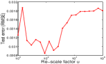
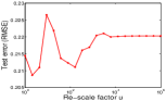
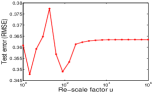
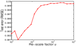
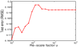
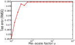
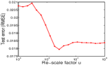
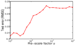
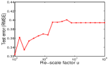
Figure 1: $L_{2}$-RBoosting test error (RMSE) curve with respect to the re-scale factor $u$. Three rows denote the 1-dimension regression functions $m_{1},m_{2},m_{3}$ and three columns indicate the noise level $\sigma$ varies among in $\{0,0.5,1\}$, respectively.

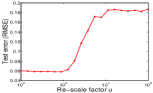
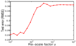
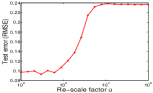
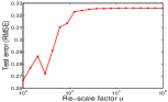
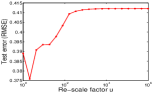
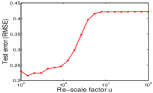
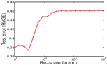
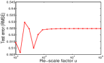
Figure 2: Three rows denote the 2-dimension regression functions $m_{4},m_{5},m_{6}$ and three columns indicate the noise level $\sigma$ varies among in $\{0,0.5,1\}$, respectively.

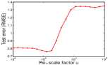
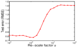
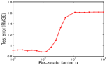
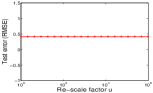
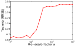
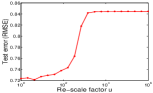
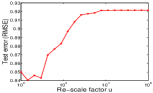
Figure 3: Three rows denote the 1-dimension regression functions $m_{7},m_{8},m_{9}$ and three columns indicate the noise level $\sigma$ varies among in $\{0,0.5,1\}$, respectively.

formance curves generally imply that there exists an optimal $u$, which may be not unique, to minimize the generalization error. This is consistent with our theoretical assertions. For $m_{8}$, the test error curve of $L_{2}$-RBoosting is “flat” with respect to $u$, that is, the generalization performance of $L_{2}$-RBoosting is irrelevant with $u$. As the uniqueness of the optimal $u$ is not imposed, such numerical observations do not count our previous theoretical conclusion. The reason can be concluded as follows. The first one is that in Theorem III.1, we impose a relatively strong restriction to the regression function and $m_{8}$ might be not satisfy it. The other one is that the adopted weak learner is too strong (we pre-set the number of splits $J=4$). Over grown tree trained on all samples are liable to autocracy and re-scale operation does not bring performance benefits at all in such case. All these numerical results illustrate the importance of selecting an appropriate shrinkage degree in $L_{2}$-RBoosting.

IV-A3 Performance comparison of $L_{2}$-Boosting, $L_{2}$-RBoosting and $L_{2}$-DDRBoosting

In this part, we compare the learning performances among $L_{2}$-Boosting, $L_{2}$-RBoosting and $L_{2}$-DDRBoosting. Table I-Table III document the generalization errors (RMSE) of $L_{2}$-Boosting, $L_{2}$-RBoosting and $L_{2}$-DDRBoosting for regression functions $m_{1},\dots,m_{9}$, respectively (the bold numbers denote the optimal performance). The standard errors are also reported (numbers in parentheses).

Form the tables we can get clear results that except for the noiseless 1-dimensional cases, the performance of $L_{2}$-RBoosting dominates both $L_{2}$-Boosting and $L_{2}$-DDRBoosting for all regression functions by a large margin. Through this series of numerical studies, including 27 different learning tasks, firstly, we verify the second guidance deduced from Thm.I that $L_{2}$-RBoosting outperforms $L_{2}$-Boosting with finite sample available. Secondly, although $L_{2}$-DDRBoosting can perfectly solve the parameter selection problem in the re-scale-type boosting algorithm, the table results also illustrate that $L_{2}$-RBoosting endows better performance once an appropriate $u$ is selected.

IV-A4 Adaptive parameter-selection strategy for shrinkage degree

We employ the simulations to verify the feasibility of the proposed parameter-selection strategy. As described in subsection 3.3, we random split the train samples $D_{m}=(X_{i},Y_{i})_{i=1}^{500}$ into two disjoint equal size subsets, i.e., a learning set and a validation set. We first train on the learning set $D^{l}_{m}$ to construct the $L_{2}$-RBoosting estimates $f_{D^{l}_{m},\alpha_{k},k}$ and then use the validation set $D^{v}_{m}$ to choose the appropriate shrinkage degree $\alpha^{*}_{k}$ and iteration $k^{*}$ by minimizing the validation risk. Thirdly, we retrain the obtained $\alpha^{*}_{k}$ on the entire training set $D_{m}$ to construct $f_{D_{m},\alpha^{*}_{k},k}$ (Generally, if we have enough training samples at hand, this step is optional). Finally, an independent test set of 1000 noiseless observations are used to evaluate the performance of $f_{D_{m},\alpha^{*}_{k},k}$.

Table IV-Table VI document the test errors (RMSE) for regression functions $m_{1},\dots,m_{9}$. The corresponding bold numbers denote the ideal generalization performance of the $L_{2}$-RBoosting (choose optimal iteration $k^{*}$ and optimal shrinkage degree $\alpha^{*}_{k}$ both according to minimize the test error via the test sets). We also report the standard errors (numbers in parentheses) of selected re-scale parameter $u$ over 20 independent runs in order to check the stability of such parameter-selection strategy. From the tables, we can easily find that the performance with such strategy approximates the ideal one. More important, comparing the mean values and standard errors of $u$ with the performance curves in Fig.1-Fig.3, apart from $m_{8}$, we can distinctly detect that the selected $u$ values by the proposed parameter-selection strategy are all located near the low valleys.

TABLE I: Performance comparison of $L_{2}$-Boosting, $L_{2}$-RBoosting and $L_{2}$-DDRBoosting on simulated regression data sets (1-dimension cases).

	$m_{1}$	$m_{2}$	$m_{3}$
$\sigma=0$
Boosting	0.0318(0.0069)	0.0895(0.0172)	0.0184(0.0025)
RBoosting	0.0308(0.0047)	0.0810(0.0183)	0.0179(0.0004)
DDRBoosting	0.0268(0.0062)	0.0747(0.0232)	0.0178(0.0011)
$\sigma=0.5$
Boosting	0.2203(0.0161)	0.1925(0.0293)	0.2507(0.0336)
RBoosting	0.2087(0.0181)	0.1665(0.0210)	0.2051(0.0252)
DDRBoosting	0.2388(0.0114)	0.2142(0.0519)	0.2508(0.0179)
$\sigma=1$
Boosting	0.3635(0.0467)	0.2943(0.0375)	0.3943(0.0415)
RBoosting	0.3479(0.0304)	0.2558(0.0120)	0.3243(0.0355)
DDRBoosting	0.3630(0.0315)	0.3787(0.0614)	0.4246(0.0360)

TABLE II: Performance comparison of $L_{2}$-Boosting, $L_{2}$-RBoosting and $L_{2}$-DDRBoosting on simulated regression data sets (2-dimension cases).

	$m_{4}$	$m_{5}$	$m_{6}$
$\sigma=0$
Boosting	0.2125(0.0173)	0.2391(0.0140)	0.3761(0.0235)
RBoosting	0.0582(0.0051)	0.0930(0.0133)	0.2161(0.0763)
ARBoosting	0.1298(0.0167)	0.1883(0.0216)	0.3585(0.0573)
$\sigma=0.5$
Boosting	0.3646(0.0152)	0.3693(0.0111)	0.4658(0.0233)
RBoosting	0.2392(0.0223)	0.2665(0.0163)	0.3738(0.0323)
ARBoosting	0.3439(0.0317)	0.3344(0.0117)	0.5100(0.0788)
$\sigma=1$
Boosting	0.5250(0.0323)	0.3967(0.0317)	0.5966(0.0424)
RBoosting	0.3836(0.0182)	0.3759(0.0231)	0.5066(0.0701)
ARBoosting	0.4918(0.0209)	0.4036(0.0180)	0.5638(0.0450)

TABLE III: Performance comparison of $L_{2}$-Boosting, $L_{2}$-RBoosting and $L_{2}$-DDRBoosting on simulated regression data sets (10-dimension cases).

	$m_{7}$	$m_{8}$	$m_{9}$
$\sigma=0$
Boosting	1.4310(0.0412)	0.4167(0.0324)	0.8274(0.0142)
RBoosting	0.7616(0.0144)	0.4167(0.0403)	0.6875(0.0107)
DDRBoosting	1.1322(0.0696)	0.4178(0.0409)	0.8130(0.0330)
$\sigma=0.5$
Boosting	1.4450(0.0435)	0.4283(0.0314)	0.8579(0.0414)
RBoosting	0.7755(0.0475)	0.4283(0.0401)	0.7218(0.0223)
DDRBoosting	1.2526(0.0290)	4381(0.0304)	0.8385(0.0222)
$\sigma=1$
Boosting	1.4420(0.0413)	0.4404(0.0242)	0.8579(0.0415)
RBoosting	0.8821(0.0575)	0.4404(0.0321)	0.8406(0.0175)
DDRBoosting	1.4423(0.0625)	0.4503(0.0393)	0.9295(0.0120)

TABLE IV: Performance of $L_{2}$-RBoosting via parameter-selection strategy on simulated regression data sets (1-dimension case).

	$m_{1}$	$u$	$m_{2}$	$u$	$m_{3}$	$u$
$\sigma=0$	0.0317(0.0069)	158(164)	0.0791(0.0262)	$5(2)$	0.0180(0.0013)	$232(95)$
	0.0308(0.0062)		0.0747(0.0232)		0.0178(0.0011)
$\sigma=0.5$	0.2113(0.0122)	609(160)	0.1766(0.0135)	$3(3)$	0.2118(0.0094)	$3(2)$
	0.2087(0.0181)		0.1665(0.0210)		0.2051(0.0252)
$\sigma=1$	0.3487(0.0132)	$987(440)$	0.2800(0.0308)	$1(0)$	0.3302(0.0511)	$148(400)$
	0.3479(0.0304)		0.2558(0.0120)		0.3243(0.0355)

TABLE V: Performance of $L_{2}$-RBoosting via parameter-selection strategy on simulated regression data sets (2-dimension case).

	$m_{4}$	$u$	$m_{5}$	$u$	$m_{6}$	$u$
$\sigma=0$	0.0593(0.0059)	55(34)	0.0958(0.0063)	$10(8)$	0.2210(0.0143)	$3(2)$
	0.0582(0.0051)		0.0930(0.0133)		0.2161(0.0763)
$\sigma=0.5$	0.2511(0.0130)	4(3)	0.2848(0.0201)	$142(300)$	0.3869(0.0173)	$20(30)$
	0.2392(0.0223)		0.2665(0.0163)		0.3738(0.0323)
$\sigma=1$	0.4001(0.0179)	$6(7)$	0.4007(0.0170)	$2(1)$	0.5123(0.0925)	$6(7)$
	0.3836(0.0182)		0.3759(0.0231)		0.5066(0.0701)

TABLE VI: Performance of $L_{2}$-RBoosting via parameter-selection strategy on simulated regression data sets (10-dimension case).

	$m_{7}$	$u$	$m_{8}$	$u$	$m_{9}$	$u$
$\sigma=0$	0.7765(0.0259)	66(65)	0.4169(0.0313)	$\diagdown$	0.6882(0.0113)	$42(36)$
	0.7616(0.0144)		0.4167(0.0403)		0.6875(0.0107)
$\sigma=0.5$	0.7757(0.0128)	72(59)	0.4349(0.0335)	$\diagdown$	0.7396(0.0145)	$11(9)$
	0.7755(0.0475)		0.4283(0.0401)		0.7218(0.0223)
$\sigma=1$	0.9093(0.0304)	$38(37)$	0.4452(0.0308)	$\diagdown$	0.8539(0.0278)	$23(30)$
	0.8821(0.0575)		0.4404(0.0321)		0.8406(0.0175)

IV-B Real data experiments

We have verified that $L_{2}$-RBoosting outperforms $L_{2}$-Boosting and $L_{2}$-DDRBoosting on the $3\times 9=27$ different distributions in the previous simulations. We now further compare the learning performances of these boosted-type algorithms on six real data sets.

The first data set is a subset of the Shanghai Stock Price Index (SSPI), which can be extracted from http://www.gw.com.cn. This data set contains 2000 trading days’ stock index which records five independent variables, i.e., maximum price, minimum price, closing price, day trading quota, day trading volume, and one dependent variable, i.e., opening price. The second one is the Diabetes data set[11]. This data set contains 442 diabetes patients that were measured on ten independent variables, i.e., age, sex, body mass index etc. and one response variable, i.e., a measure of disease progression. The third one is the Prostate cancer data set derived from a study of prostate cancer by Blake et al.[37]. The data set consists of the medical records of 97 patients who were about to receive a radical prostatectomy. The predictors are eight clinical measures, i.e., cancer volume, prostate weight, age etc. and one response variable, i.e., the logarithm of prostate-specific antigen. The fourth one is the Boston Housing data set created form a housing values survey in suburbs of Boston by Harrison[38]. This data set contains 506 instances which include thirteen attributions, i.e., per capita crime rate by town, proportion of non-retail business acres per town, average number of rooms per dwelling etc. and one response variable, i.e., median value of owner-occupied homes. The fifth one is the Concrete Compressive Strength (CCS) data set created from[39]. The data set contains 1030 instances including eight quantitative independent variables, i.e., age and ingredients etc. and one dependent variable, i.e., quantitative concrete compressive strength. The sixth one is the Abalone data set, which comes from an original study in [40] for predicting the age of abalone from physical measurements. The data set contains 4177 instances which were measured on eight independent variables, i.e., length, sex, height etc. and one response variable, i.e., the number of rings.

Similarly, we divide all the real data sets into two disjoint equal parts (except for the Prostate Cancer data set, which were divided into two parts beforehand: a training set with 67 observations and a test set with 30 observations). The first half serves as the training set and the second half serves as the test set. For each real data experiment, weak learners are changed to the decision stumps (specifying one split of each tree, $J=1$) corresponding to an additive model with only main effects. Table VII documents the performance (test RMSE) comparison results of $L_{2}$-Boosting, $L_{2}$-RBoosting and $L_{2}$-DDRBoosting on six real data sets, respectively (the bold numbers denote the optimal performance). It is observed from the table that the performance of $L_{2}$-RBoosting with $u$ selected via our recommended strategy outperforms both $L_{2}$-Boosting and $L_{2}$-DDRBoosting on all real data sets, especially for some data sets, i.e., Diabetes, Prostate and CCS, makes a great improvement.

TABLE VII: Performance comparison of $L_{2}$-Boosting, $L_{2}$-RBoosting and $L_{2}$-DDRBoosting on real data sets

	Stock	Diabetes	Prostate	Housing	CCS	Abalone
Boosting	0.0050	60.5732	0.6344	0.6094	0.7177	2.1635
RBoosting	0.0047	55.0137	0.4842	0.6015	0.6379	2.1376
DDRBoosting	0.0049	59.3595	0.6133	0.6281	0.6977	2.1849

V Proofs

In this section, we provide the proofs of the main results. At first, we aim to prove Theorem III.1. To this end, we shall give an error decomposition strategy for $\mathcal{E}(\pi_{M}f_{k})-\mathcal{E}(f_{\rho})$. Using the similar methods that in [26, 41], we construct an $f_{k}^{*}\in\mbox{span}(D_{n})$ as follows. Since $f_{\rho}\in\mathcal{L}_{1}^{r}$, there exists a $h_{\rho}:=\sum_{i=1}^{n}a_{i}g_{i}\in\mbox{span}(S)$ such that

$$\|h_{\rho}\|_{\mathcal{L}_{1}}\leq\mathcal{B},\ \mbox{and}\ \|f_{\rho}-h_{\rho}\|\leq\mathcal{B}n^{-r}.$$ (V.1)

Define

$$f_{0}^{*}=0,\ f_{k}^{*}=\left(1-\frac{1}{k}\right)f^{*}_{k-1}+\frac{\sum_{i=1}^{n}|a_{i}|\|g_{i}\|_{\rho}}{k}g^{*}_{k},$$ (V.2)

where

$$g_{k}^{*}:=\arg\max\limits_{g\in S^{\prime}}\left\langle h_{\rho}-\left(1-\frac{1}{k}\right)f_{k-1}^{*},g\right\rangle_{\rho},$$

and

$$\mathcal{D}_{n}^{\prime}:=\left\{{g_{i}(x)}/{\|g_{i}\|_{\rho}}\right\}_{i=1}^{n}\bigcup\left\{-{g_{i}(x)}/{\|g_{i}\|_{\rho}}\right\}_{i=1}^{n}$$

with $g_{i}\in S$.

Let $f_{k}$ and $f_{k}^{*}$ be defined as in Algorithm 2 and (V.2), respectively. We have

$$\mathcal{E}(\pi_{M}f_{k})-\mathcal{E}(f_{\rho})$$

$$\leq \mathcal{E}(f_{k}^{*})-\mathcal{E}(f_{\rho})+\mathcal{E}_{\bf z}(\pi_{M}f_{,k})-\mathcal{E}_{D}(f_{k}^{*})$$

$$+ \mathcal{E}_{D}(f_{k}^{*})-\mathcal{E}(f_{k}^{*})+\mathcal{E}(\pi_{M}f_{k})-\mathcal{E}_{D}(f_{k}).$$

Upon making the short hand notations

$$\mathcal{D}(k):=\mathcal{E}(f_{k}^{*})-\mathcal{E}(f_{\rho}),$$

$$\mathcal{S}(D,k):=\mathcal{E}_{D}(f_{k}^{*})-\mathcal{E}(f_{k}^{*})+\mathcal{E}(\pi_{M}f_{k})-\mathcal{E}_{D}(\pi_{M}f_{k}),$$

and

$$\mathcal{P}(D,k):=\mathcal{E}_{D}(\pi_{M}f_{k})-\mathcal{E}_{D}(f_{k}^{*})$$

respectively for the approximation error, sample error and hypothesis error, we have

$$\mathcal{E}(\pi_{M}f_{k})-\mathcal{E}(f_{\rho})=\mathcal{D}(k)+\mathcal{S}(D,k)+\mathcal{P}(D,k).$$ (V.3)

To bound estimate $\mathcal{D}(k)$, we need the following Lemma V.1, which can be found in [26, Prop.1].

Lemma V.1

Let $f_{k}^{*}$ be defined in (V.2). If $f_{\rho}\in\mathcal{L}_{1}^{r}$, then

$$\mathcal{D}(k)\leq\mathcal{B}^{2}(k^{-1/2}+n^{-r})^{2}.$$ (V.4)

To bound the hypothesis error, we need the following two lemmas. The first one can be found in [12], which is a direct generalization of [17, Lemma 2.3].

Lemma V.2

Let $j_{0}>2$ be a natural number. Suppose that three positive numbers $c_{1}<c_{2}\leq j_{0}$, $\mathcal{C}_{0}$ be given. Assume that a sequence $\{a_{n}\}_{n=1}^{\infty}$ has the following two properties:

(i) For all $1\leq n\leq j_{0}$,

$$a_{n}\leq\mathcal{C}_{0}n^{-c_{1}},$$

and, for all $n\geq j_{0}$,

$$a_{n}\leq a_{n-1}+\mathcal{C}_{0}(n-1)^{-c_{1}}.$$

(ii) If for some $v\geq j_{0}$ we have

$$a_{v}\geq\mathcal{C}_{0}v^{-c_{1}},$$

then

$$a_{v+1}\leq a_{v}(1-c_{2}/v).$$

Then, for all $n=1,2,\dots,$ we have

$$a_{n}\leq 2^{1+\frac{c_{1}^{2}+c_{1}}{c_{2}-c_{1}}}\mathcal{C}_{0}n^{-c_{1}}.$$

The second one can be easily deduced from [17, Lemma 2.2].

Lemma V.3

Let $h\in\mbox{span}(S),$ $f_{,k}$ be the estimate defined in Algorithm 2 and $y(\cdot)$ is an arbitrary function satisfying $y(x_{i})=y_{i}$. Then, for arbitrary $k=1,2,\dots$, we have

$$\|f_{k}-y\|_{m}\leq\|f_{k-1}-y\|_{m}$$

$$\left(\!1\!-\!\alpha_{k}\!\left(1\!-\!\frac{\|y-h\|_{m}}{\|f_{k-1}-y\|_{m}}\!\right)\!+\!2\left(\frac{\alpha_{k}(\|y\|_{m}+\!\|h\|_{\mathcal{L}_{1}(S)})}{(1-\alpha_{k})\|f_{k-1}-y\|_{m}}\right)^{2}\!\right).$$

Now, we are in a position to present the hypothesis error estimate.

Lemma V.4

Let $f_{k}$ be the estimate defined in Algorithm 2. Then, for arbitrary $h\in\mbox{span}(S)$ and $u\in\mathcal{N}$, there holds

$$\|f_{k}-y\|_{m}^{2}\leq 2\|y-h\|_{m}^{2}+2(M+\|h\|_{\mathcal{L}_{1}(S)})^{2}2^{\frac{3u^{2}+14u+20}{8u+8}}k^{-1}.$$

Proof:

By Lemma V.3, for $k\geq 1$, we obtain

$$\|f_{k}-y\|_{m}-\|y-h\|_{m}\leq$$

$$(1-\alpha_{k})(\|f_{k-1}-y\|_{m}-\|y-h\|_{m})$$

$$+C\|f_{k-1}-y\|_{m}\left(\frac{\alpha_{k}(\|y\|_{m}+\|h\|_{\mathcal{L}_{1}(S)})}{\|f_{k-1}-y\|_{m}}\right)^{2}.$$

Let

$$a_{k+1}=\|f_{k}-y\|_{m}-\|y-h\|_{m}.$$

Then, by noting $\|y\|_{m}\leq M$, we have

$$a_{k+1}\leq(1-\alpha_{k})a_{k}+C\frac{\alpha_{k}^{2}(M+\|h\|_{\mathcal{L}_{1}(S)})^{2}}{a_{k}}.$$

We plan to apply Lemma V.2 to the sequence $\{a_{n}\}$. Let $\mathcal{C}_{0}=\max\{1,\sqrt{C}\}2(M+\|h\|_{l^{1}(\mathcal{D}_{n})})$ According to the definitions of $\{a_{k}\}_{k=1}^{\infty}$ and $f_{k}$, we obtain

$$a_{1}=\|y\|_{m}-\|y-h\|_{m}\leq 2M+\|h\|_{\mathcal{L}_{1}(S)}\leq\mathcal{C}_{0},$$

and

$$a_{k+1}\leq a_{k}+\alpha_{k}\|y\|_{m}\leq a_{k}+\mathcal{C}_{0}k^{-1/2}.$$

Let $a_{k}\geq\mathcal{C}_{0}k^{-1/2}$, since $\alpha_{k}=\frac{2}{k+u}$, we then obtain

$$a_{k}\leq\frac{k+u-2}{k+u}a_{k-1}+Ca_{k-1}k\frac{4}{\mathcal{C}_{0}^{2}(k+u)^{2}}(M+\|h\|_{\mathcal{L}_{1}(S)})^{2}.$$

That is,

$$a_{k}\leq a_{k-1}\left(1-\frac{2}{k+u}+C\frac{4k}{\mathcal{C}_{0}^{2}(k+u)^{2}}(M+\|h\|_{\mathcal{L}_{1}(S)})^{2}\right)$$

$$\leq(1-\left(\frac{1}{2}+\frac{2u+2}{(2+u)^{2}}\right)\frac{1}{k-1}).$$

Now, it follows from Lemma V.2 with $c_{1}=\frac{1}{2}$ and $c_{2}=\frac{1}{2}+\frac{2u+2}{(2+u)^{2}}$ that

$$a_{n}\leq\max\{1,\sqrt{C}\}2(M+\|h\|_{\mathcal{L}_{1}(S)})2^{1+\frac{3(u+2)^{2}}{8u+8}}n^{-1/2}.$$

Therefore, we obtain

$$\|f_{k}-y\|_{m}\leq\|y-h\|_{m}+(M+\|h\|_{\mathcal{L}_{1}(S)})2^{\frac{3u^{2}+14u+20}{8u+8}}k^{-1/2}.$$

This finishes the proof of Lemma V.4. ∎

Now we proceed the proof of Theorem III.1.

Proof:

Based on Lemma V.4 and the fact $\|f^{*}_{k}\|_{\mathcal{L}_{1}(S)}\leq\mathcal{B}$ [26, Lemma 1], we obtain

$$\mathcal{P}(D,k)\leq 2\mathcal{E}_{D}(\pi_{M}f_{k})-\mathcal{E}_{D}(f_{k}^{*})\leq 2(M+\mathcal{B})^{2}2^{\frac{3u^{2}+14u+20}{8u+8}}k^{-1}.$$ (V.5)

Therefore, both the approximation error and hypothesis error are deduced. The only thing remainder is to bound bound the sample error $\mathcal{S}(D,k)$. Upon using the short hand notations

$$S_{1}(D,k):=\{\mathcal{E}_{D}(f_{k}^{*})-\mathcal{E}_{D}(f_{\rho})\}-\{\mathcal{E}(f_{k}^{*})-\mathcal{E}(f_{\rho})\}$$

and

$$S_{2}(D,k):=\{\mathcal{E}(\pi_{M}f_{k})-\mathcal{E}(f_{\rho})\}-\{\mathcal{E}_{D}(\pi_{M}f_{k})-\mathcal{E}_{D}(f_{\rho})\},$$

we write

$$\mathcal{S}(D,k)=\mathcal{S}_{1}(D,k)+\mathcal{S}_{2}(D,k).$$ (V.6)

It can be found in [26, Prop.2] that for any $0<t<1$, with confidence $1-\frac{t}{2}$,

$$\mathcal{S}_{1}(D,k)\leq\frac{7(3M+\mathcal{B}\log\frac{2}{t})}{3m}+\frac{1}{2}\mathcal{D}(k)$$ (V.7)

It also follows from [42, Eqs(A.10)] that

$$\mathcal{S}_{2}(D,k)\leq\frac{1}{2}\mathcal{E}(\pi_{M}f_{k})-\mathcal{E}(f_{\rho})+\log\frac{2}{t}\frac{Ck\log m}{m}$$ (V.8)

holds with confidence at least $1-t/2$. Therefore, (V.3), (V.4), (V.5), (V.6), (V.7) and (V.8) yield that

$$\mathcal{E}(\pi_{M}f_{k})-\mathcal{E}(f_{\rho})\leq$$

$$C(M\!+\!\mathcal{B})^{2}\left(2^{\frac{3u^{2}+14u+20}{8u+8}}k^{-1}\!+\!(m/k)^{-1}\log m\log\frac{2}{t}+n^{-2r}\!\right)$$

holds with confidence at least $1-t$. This finishes the proof of Theorem III.1. ∎

Proof:

It can be deduced from [17, Theorem 1.2] and the same method as in the proof of Theorem III.1. For the sake of brevity, we omit the details. ∎

Proof:

It is easy to check that

$$f_{k}=(1-\alpha_{k})f_{k-1}+\langle y-(1-\alpha_{k})f_{k-1},g_{k}\rangle_{2}g_{k}.$$

As $\|g_{k}\|\leq 1$, we obtain from the Hölder inequality that

$$\langle y-(1-\alpha_{k})f_{k-1},g_{k}\rangle_{2}\leq\|y-(1-\alpha_{k})f_{k-1}\|_{2}$$

$$\leq(1-\alpha_{k})\|y-f_{k-1}\|_{2}+\alpha_{k}M.$$

As

$$\|y-f_{k-1}\|_{2}\leq C(M+\|h\|_{\mathcal{L}_{1}(S)})k^{-1/2}+n^{-r},$$

we can obtain

$$\|f_{k}\|_{1}\leq C((M+\|h\|_{\mathcal{L}_{1}(S)})k^{1/2}+kn^{-r}).$$

This finishes the proof of Proposition III.3. ∎

Now we turn to prove Theorem III.7. The following concentration inequality [43] plays a crucial role in the proof.

Lemma V.5

Let $\mathcal{F}$ be a class of measurable functions on $Z$. Assume that there are constants $B,c>0$ and $\alpha\in[0,1]$ such that $\|f\|_{\infty}\leq B$ and $\mathbf{E}f^{2}\leq c(\mathbf{E}f)^{\alpha}$ for every $f\in\mathcal{F}.$ If for some $a>0$ and $\mu\in(0,2)$,

$$\log\mathcal{N}_{2}(\mathcal{F},\varepsilon)\leq a\varepsilon^{-\mu},\ \ \forall\varepsilon>0,$$ (V.9)

then there exists a constant $c_{p}^{\prime}$ depending only on $p$ such that for any $t>0$, with probability at least $1-e^{-t}$, there holds

$$\mathbf{E}f-\frac{1}{m}\sum_{i=1}^{m}f(z_{i})\leq$$ (V.10)

$$\frac{1}{2}\eta^{1-\alpha}(\mathbf{E}f)^{\alpha}+c_{\mu}^{\prime}\eta+2\left(\frac{ct}{m}\right)^{\frac{1}{2-\alpha}}+\frac{18Bt}{m},\ \forall f\in\mathcal{F},$$

where

$$\eta:=\max\left\{c^{\frac{2-\mu}{4-2\alpha+\mu\alpha}}\left(\frac{a}{m}\right)^{\frac{2}{4-2\alpha+\mu\alpha}},B^{\frac{2-\mu}{2+\mu}}\left(\frac{a}{m}\right)^{\frac{2}{2+\mu}}\right\}.$$

We continue the proof of Theorem III.7.

Proof:

For arbitrary $h\in\mbox{span}(S)$,

$$\mathcal{E}(f_{k})-\mathcal{E}(h)= \mathcal{E}(f_{k})-\mathcal{E}(h)-(\mathcal{E}_{D}(f_{k})-\mathcal{E}_{D}(h))$$

$$+\mathcal{E}_{D}(f_{k})-\mathcal{E}_{D}(h).$$

Set

$$\mathcal{G}_{R}:=\left\{g(z)=(\pi_{M}f(x)-y)^{2}-(h(x)-y)^{2}:f\in B_{R}\right\}.$$ (V.11)

Using the obvious inequalities $\|\pi_{M}f\|_{\infty}\leq M$, $|y|\leq M$ a.e., we get the inequalities

$$|g(z)|\leq(3M+\|h\|_{\mathcal{L}_{1}(S)})^{2}$$

and

$$\mathbf{E}g^{2}\leq(3M+\|h\|_{\mathcal{L}_{1}(S)})^{2}\mathbf{E}g.$$

For $g_{1},g_{2}\in\mathcal{G}_{R}$, it follows that

$$|g_{1}(z)-g_{2}(z)|\leq(3M+\|h\|_{\mathcal{L}_{1}(S)})|f_{1}(x)-f_{2}(x)|.$$

Then

$$\mathcal{N}_{2}(\mathcal{G}_{R},\varepsilon)\leq\mathcal{N}_{2,{\bf x}}\left(B_{R},\frac{\varepsilon}{3M+\|h\|_{\mathcal{L}_{1}(S)}}\right)$$

$$\leq\mathcal{N}_{2,{\bf x}}\left(B_{1},\frac{\varepsilon}{R(3M+\|h\|_{\mathcal{L}_{1}(S)})}\right).$$

Using the above inequality and Assumption III.6, we have

$$\log\mathcal{N}_{2}(\mathcal{F}_{R},\varepsilon)\leq\mathcal{L}(R(3M+\|h\|_{\mathcal{L}_{1}(S)}))^{\mu}\varepsilon^{-\mu}.$$

By Lemma V.5 with $B=c=(3M+\|h\|_{\mathcal{L}_{1}(S)})^{2}$, $\alpha=1$ and $a=\mathcal{L}(R(3M+\|h\|_{1}))^{\mu}$, we know that for any $t\in(0,1),$ with confidence $1-\frac{t}{2},$ there exists a constant $C$ depending only on $d$ such that for all $g\in\mathcal{G}_{R}$

$$\mathbf{E}g-\frac{1}{m}\sum_{i=1}^{m}g(z_{i})\leq\frac{1}{2}\mathbf{E}g+c_{\mu}^{\prime}\eta+20(3M+\|h\|_{\mathcal{L}_{1}(S)})^{2}\frac{\log 4/t}{m}.$$

Here

$$\eta=((3M+\|h\|_{\mathcal{L}_{1}(S)})^{2})^{\frac{2-\mu}{2+\mu}}\left(\frac{\mathcal{L}(R(3M+\|h\|_{\mathcal{L}_{1}(S)}))^{\mu}}{m}\right)^{\frac{2-\mu}{2+\mu}}.$$

It then follows from Proposition III.3 that

$$\mathcal{E}(f_{k})-\mathcal{E}(f_{\rho})\leq$$

$$C\log\frac{2}{t}(3M+\mathcal{B})^{2}\left(n^{-2r}+k^{-1}+\left(\frac{(kn^{-r}+\sqrt{k})^{\mu}}{m}\right)^{\frac{2-\mu}{2+\mu}}\right).$$

This finishes the proof of Theorem III.7. ∎

VI Conclusion

In this paper, we draw a concrete analysis concerning how to determine the shrinkage degree into $L_{2}$-RBoosting. The contributions can be concluded in four aspects. Firstly, we theoretically deduced the generalization error bound of $L_{2}$-RBoosting and demonstrated the importance of the shrinkage degree. It is shown that, under certain conditions, the learning rate of $L_{2}$-RBoosting can reach $O(m^{-1/2}\log m)$, which is the same as the optimal “record” for greedy learning and boosting-type algorithms. Furthermore, our result showed that although the shrinkage degree did not affect the learning rate, it determined the constant of the generalization error bound, and therefore, played a crucial role in $L_{2}$-RBoosting learning with finite samples. Then, we proposed two schemes to determine the shrinkage degree. The first one is the conventional parameterized $L_{2}$-RBoosting, and the other one is to learn the shrinkage degree from the samples directly ($L_{2}$-DDRBoosting). We further provided the theoretically optimality of these approaches. Thirdly, we compared these two approaches and proved that, although $L_{2}$-DDRBoosting reduced the parameters, the estimate deduced from $L_{2}$-RBoosting possessed a better structure ($l^{1}$ norm). Therefore, for some special weak learners, $L_{2}$-RBoosting can achieve better performance than $L_{2}$-DDRBoosting. Fourthly, we developed an adaptive parameter-selection strategy for the shrinkage degree. Our theoretical results demonstrated that, $L_{2}$-RBoosting with such a shrinkage degree selection strategy did not degrade the generalization capability very much. Finally, a series of numerical simulations and real data experiments have been carried out to verify our theoretical assertions. The obtained results enhanced the understanding of RBoosting and could provide guidance on how to utilize $L_{2}$-RBoosting for regression tasks.

References

- [1] J. Friedman, “Greedy function approximation: a gradient boosting machine,” Ann. Stat., vol. 29, no. 5, pp. 1189–1232, 2001.
- [2] P. Buhlmann and B. Yu, “Boosting with the loss: regression and classification,” J. Amer. Stat. Assoc., vol. 98, no. 462, pp. 324–339, 2003.
- [3] Y. Freund and R. E. Schapire, “Experiments with a new boosting algorithm,” ICML, vol. 96, pp. 148–156, 1996.
- [4] J. Friedman, T. Hastie, and R. Tibshirani, “Additive logistic regression: a statistical view of boosting (with discussion and a rejoinder by the authors),” Ann. Stat., vol. 28, no. 2, pp. 337–407, 2000.
- [5] P. Buhlmann and T. Hothorn, “Boosting algorithms: regularization, prediction and model fitting,” Stat. Sci., vol. 22, no. 4, pp. 477–505, 2007.
- [6] N. Duffy and D. Helmbold, “Boosting methods for regression,” Mach. Learn., vol. 47, no. 2-3, pp. 153–200, 2002.
- [7] Y. Freund, “Boosting a weak learning algorithm by majority,” Inform. Comput., vol. 121, no. 2, pp. 256–285, 1995.
- [8] R. E. Schapire, “The strength of weak learnability,” Mach. Learn., vol. 5, no. 2, pp. 1997–2027, 1990.
- [9] P. Bartlett and M. Traskin, “Adaboost is consistent,” J. Mach. Learn. Res., vol. 8, pp. 2347–2368, 2007.
- [10] E. D. Livshits, “Lower bounds for the rate of convergence of greedy algorithms,” Izvestiya: Mathematics, vol. 73, no. 6, pp. 1197–1215, 2009.
- [11] B. Efron, T. Hastie, I. Johnstone, and R. Tibsirani, “Least angle regression,” Ann. Stat., vol. 32, no. 2, pp. 407–451, 2004.
- [12] S. B. Lin, Y. Wang, and L. Xu, “Re-scale boosting for regression and classification,” ArXiv:1505.01371, 2015.
- [13] J. Ehrlinger and H. Ishwaran, “Characterizing boosting,” Ann. Stat., vol. 40, no. 2, pp. 1074–1101, 2012.
- [14] T. Zhang and B. Yu, “Boosting with early stopping: convergence and consistency,” Ann. Stat., vol. 33, no. 4, pp. 1538–1579, 2005.
- [15] T. Hastie, J. Taylor, R. Tibshirani, and G. Walther, “Forward stagewise regression and the monotone lasso,” Electron. J. Stat., vol. 1, pp. 1–29, 2007.
- [16] P. Zhao and B. Yu, “Stagewise lasso,” J. Mach. Learn. Res., vol. 8, pp. 2701–2726, 2007.
- [17] V. Temlyakov, “Relaxation in greedy approximation,” Constr. Approx., vol. 28, no. 1, pp. 1–25, 2008.
- [18] T. Zhang, “Sequential greedy approximation for certain convex optimization problems,” IEEE Trans. Inform. Theory, vol. 49, no. 3, pp. 682–691, 2003.
- [19] J. Elith, J. R. Leathwick, and T. Hastie, “A working guide to boosted regression trees,” J. Anim. Ecol., vol. 77, no. 4, pp. 802–813, 2008.
- [20] L. Breiman, “Bagging predictors,” Mach. Learn., vol. 24, no. 2, pp. 123–140, 1996.
- [21] P. Smyth and D. Wolpert, “Linearly combining density estimators via stacking,” Mach. Learn., vol. 36, no. 1-2, pp. 59–83, 1999.
- [22] D. MacKay, “Bayesian methods for adaptive models,” PhD thesis, California Institute of Technology, 1991.
- [23] L. Breiman, “Random forests,” Mach. Learn., vol. 45, no. 1, pp. 5–32, 2001.
- [24] A. Bagirov, C. Clausen, and M. Kohler, “An boosting algorithm for estimation of a regression function,” IEEE Trans. Inform. Theory, vol. 56, no. 3, pp. 1417–1429, 2010.
- [25] P. Bickel, Y. Ritov, and A. Zakai, “Some theory for generalized boosting algorithms,” J. Mach. Learn. Res., vol. 7, pp. 705–732, 2006.
- [26] S. B. Lin, Y. H. Rong, X. P. Sun, and Z. B. Xu, “Learning capability of relaxed greedy algorithms,” IEEE Trans. Neural Netw. Learn. Syst., vol. 24, no. 10, pp. 1598–1608, 2013.
- [27] R. DeVore and V. Temlyakov, “Some remarks on greedy algorithms,” Adv. Comput. Math., vol. 5, no. 1, pp. 173–187, 1996.
- [28] V. Temlyakov, “Greedy approximation,” Acta Numer., vol. 17, pp. 235–409, 2008.
- [29] A. Barron, A. Cohen, W. Dahmen, and R. DeVore, “Approximation and learning by greedy algorithms,” Ann. Stat., vol. 36, no. 1, pp. 64–94, 2008.
- [30] L. Xu, S. B. Lin, Y. Wang, and Z. B. Xu, “A comparison study between different re-scale boosting,” Manuscript, 2015.
- [31] V. Temlyakov, “Greedy approximation in convex optimization,” Constr. Approx., pp. 1–28, 2012.
- [32] D. X. Zhou and K. Jetter, “Approximation with polynomial kernels and svm classifiers,” Adv. Comput. Math., vol. 25, no. 1-3, pp. 323–344, 2006.
- [33] L. Shi, Y. L. Feng, and D.X.Zhou, “Concentration estimates for learning with -regularizer and data dependent hypothesis spaces,” Appl. Comput. Harmon. Anal., vol. 31, no. 2, pp. 286–302, 2011.
- [34] L. Györfi, M. Kohler, A. Krzyzak, and H. Walk, “A distribution-free theory of nonparametric regression,” Springer Science & Business Media, 2002.
- [35] T. Hastie, R.Tibshirani, and J. Friedman, “The elements of statistical learning,” New York: springer, 2001.
- [36] L. Breiman, J. Friedman, C. Stone, and R. Olshen, “Classification and regression trees,” CRC press, 1984.
- [37] C. Blake and C. Merz, “{UCI} repository of machine learning databases,” 1998.
- [38] D. Harrison and D. L. Rubinfeld, “Hedonic prices and the demand for clean air,” J. Environ. Econ., vol. 5, no. 1, pp. 81–102, 1978.
- [39] I. C. Ye, “Modeling of strength of high performance concrete using artificial neural networks,” Cement and Concrete Research, vol. 28, no. 12, pp. 1797–1808, 1998.
- [40] W. J. Nash, T. L. Sellers, S. R. Talbot, A. J. Cawthorn, and W. B. Ford, “The population biology of abalone (haliotis species) in tasmania. i. blacklip abalone (h. rubra) from the north coast and islands of bass strait,” Sea Fisheries Division, Technical Report, no. 48, 1994.
- [41] L. Xu, S. B. Lin, J. S. Zeng, and Z. B. Xu, “Greedy metric in orthogonal greedy learning,” Manuscript, 2015.
- [42] C. Xu, S. B. Lin, J. Fang, and R. Z. Li, “Efficient greedy learning for massive data,” Manuscript, 2014.
- [43] Q. Wu, Y. Ying, and D. X. Zhou, “Multi-kernel regularized classifiers,” J. Complex., vol. 23, no. 1, pp. 108–134, 2007.