Abstract

Connections compatible with degenerate metric structures are known to possess peculiar features: on the one hand, the compatibility conditions involve restrictions on the torsion; on the other hand, torsionfree compatible connections are not unique, the arbitrariness being encoded in a tensor field whose type depends on the metric structure. Nonrelativistic structures typically fall under this scheme, the paradigmatic example being a contravariant degenerate metric whose kernel is spanned by a one-form. Torsionfree compatible (i.e.  Galilean) connections are characterised by the gift of a two-form (the force field). Whenever the two-form is closed, the connection is said Newtonian. Such a nonrelativistic spacetime is known to admit an ambient description as the orbit space of a gravitational wave with parallel rays. The leaves of the null foliation are endowed with a nonrelativistic structure dual to the Newtonian one, dubbed Carrollian spacetime. We propose a generalisation of this unifying framework by introducing a new non-Lorentzian ambient metric structure of which we study the geometry. We characterise the space of (torsional) connections preserving such a metric structure which is shown to project to (resp. embed) the most general class of (torsional) Galilean (resp. Carrollian) connections.

1 Introduction

In contradistinction with the familiar relativistic case, the geometry of nonrelativistic spacetimes is characterised by degenerate metric structures. The princeps example of nonrelativistic spacetimes originates from Newtonian mechanics, in which time and space are assumed to be separate entities, each one being imparted with an absolute status. Both of these features can be nicely encoded in a geometric fashion [1, 2] by identifying the nonrelativistic spacetime as a manifold $\bar{\mathscr{M}}$ endowed with a metric structure ($\bar{h}^{\mu\nu}$, $\bar{\psi}_{\mu}$), where $\bar{h}^{\mu\nu}$ stands for a twice-contravariant degenerate metric whose radical is spanned by a nowhere-vanishing 1-form $\bar{\psi}_{\mu}$ (hence $\bar{h}^{\mu\nu}\bar{\psi}_{\mu}=0$). Nowadays, this construction is often referred to as Newton-Cartan geometry [3]. The 1-form $\bar{\psi}$ plays here the role of an absolute clock while the cometric $\bar{h}$ provides $\bar{\mathscr{M}}$ with a notion of spatial distance and will hence be referred to as a collection of absolute rulers. An equivalent definition of absolute rulers can be given in the form of a positive-definite metric $\bar{\gamma}$ acting on the kernel of $\bar{\psi}$. When causality is assumed (i.e.  when the absolute clock satisfies the Frobenius integrability condition $\bar{\psi}_{[\mu}\partial_{\lambda}\bar{\psi}_{\nu]}=0$), the kernel of $\bar{\psi}$ defines an integrable distribution whose integral submanifolds foliate the spacetime $\bar{\mathscr{M}}$. Each of these integral hypersurfaces can then be thought of as the absolute space at a given time on which a notion of distance is provided by the collection of absolute rulers $\bar{\gamma}$. The “metric” structure of Newtonian gravity is thus embodied in a triplet $\left(\bar{\mathscr{M}},\bar{\psi},\bar{\gamma}\right)$, referred to as a Leibnizian structure in [4, 5].

Strictly speaking, metric structures (degenerate or not) do not provide a notion of parallelism. The latter can be implemented in the guise of a compatible connection. However, connections compatible with degenerate metric structures are known [6] to differ from the usual, nondegenerate case by at least two related aspects: on the one hand, the compatibility conditions involve restrictions on the torsion so that not all torsion tensors are admissible; on the other hand, only a subset of metric structures admits a torsionfree compatible connection. Moreover, even when the existence of such a connection is ensured, its uniqueness is not and two different torsionfree compatible connections differ by a tensor field whose type depends on the metric structure. As for Leibnizian structures, the compatibility condition with the absolute clock ($\bar{\nabla}_{\mu}\bar{\psi}_{\nu}=0$) enforces the following constraint on the torsion tensor: $\bar{\psi}_{\lambda}\bar{\Gamma}{}^{\lambda}_{[\mu\nu]}=\partial_{[\mu}\bar{\psi}_{\nu]}$. Consequently, only Leibnizian structures with closed absolute clock admit torsionfree compatible connections (this subset was dubbed Augustinian structures in [5]). Consequently, when dealing with nonrelativistic metric structures with non-closed absolute clocks ($d\bar{\psi}\neq 0$), torsionfreeness and compatibility become mutually exclusive features. Furthermore, the previous constraint fixes the “timelike” part of the torsion tensor so that the gift of the latter is not sufficient to uniquely define a compatible connection and must be supplemented by a 2-form $\bar{F}_{\mu\nu}$.

When the absolute clock is closed, torsionfree compatible connections are allowed and are then completely characterised by the gift of a 2-form $\bar{F}$. The appearance of such a 2-form in the nonrelativistic context is in fact quite natural if one acknowledges the fact that in Newtonian mechanics, spacetime is a mere “container” whose structure is not rich enough to prescribe the motion of particles. In particular, when the external forces are of the Lorentz type (i.e.  $\ddot{x}^{\mu}=\bar{h}^{\mu\nu}\bar{F}_{\nu\rho}\,\dot{x}^{\rho}$), the dynamics of a single particle is specified by a force-field $\bar{F}$ (interpreted as the Faraday tensor in the electromagnetic case). Newtonian connections are torsionfree Galilean connections for which $\bar{F}$ is closed, so that locally there exists a 1-form $\bar{A}$ such that $\bar{F}=d\bar{A}$. Remarkably, this closedness property is equivalent to an algebraic condition on the curvature of the connection: the so-called Duval-Künzle condition [7, 8]. A distinctive feature of Newtonian connections is that the corresponding geodesic equation can be derived via a variational principle from a Lagrangian built in terms of the Leibnizian structure and the potential 1-form. As shown in [9, 5], such a Lagrangian defines a (possibly nondegenerate) Lagrangian metric on $\bar{\mathscr{M}}$ which reduces on the absolute spaces to the absolute collections of rulers $\bar{\gamma}$, and furthermore constitutes the necessary and sufficient structure needed to supplement a Leibnizian structure in order to define a unique Newtonian connection.

Figure 1 sums up the interrelations between the different dramatis personæ constituting the kinematical content of Newton-Cartan geometry, in complete analogy with the relativistic case:

Figure 1: Kinematical content of Newton-Cartan geometry

Besides its purely mathematical interest, Newton-Cartan geometry has recently known a revival of interest triggered first by condensed-matter applications [10, 11] following the seminal work by Son [12] (cf.  also [13] for an early inspiring work on superfluids). These structures have also made novel appearances in the active fields of Lifshitz and Schrödinger holography [14, 15] and in the context of Hořava-Lifshitz gravity [16]. Most of these recent works focus (with the exception of the work [17] which considers the general case) on a special class of torsional Galilean connection dubbed Torsional Newton-Cartan (TNC) geometries.

Newtonian structures embedded inside Bargmannian structures

Although Newtonian structures have been advocated to live on their own, new light can be shed on such structures by embedding them inside relativistic ones, thus providing naturality to seemingly peculiar nonrelativistic structures and properties by importing them from usual relativistic ones. The origin of this perspective on nonrelativistic physics can be traced back to an early work of Eisenhart [18] establishing that the dynamical trajectories of a holonomic mechanical system with $d$ degrees of freedom can be put in correspondence with the affine geodesics of a specific $d+2$ dimensional relativistic spacetime. Thus, nonrelativistic dynamical trajectories can always be “lifted” to geodesics (hence the denomination of “Eisenhart lift”) and conversely, any relativistic geodesic can be projected onto a nonrelativistic dynamical trajectory. The class of relativistic spacetimes allowing the Eisenhart lift can be characterised by the existence of a light-like vector field which is parallel with respect to the Levi-Civita connection. This class of metrics had previously been considered in [19] in a different context and later received the interpretation of gravitational waves with parallel rays [20], where the rays are the integral curves of the light-like and parallel vector field (dubbed wave vector field in the following). Such spacetimes will be referred to as Bargmann-Eisenhart waves, cf.  [21].

This bridge between nonrelativistic physics and relativistic spacetimes has been independently rediscovered afterwards by Duval and collaborators [22, 20] who generalised the “ambient” approach of Eisenhart in order to provide an account of the different levels of the kinematical and dynamical contents of Newtonian gravity as embedded inside Bargmann-Eisenhart waves.

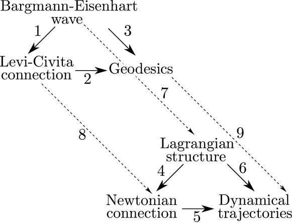
Figure 2: Newtonian structures embedded inside Bargmannian structures

The main idea underlying the ambient approach to nonrelativistic physics consists in performing a dimensional reduction of a Bargmann-Eisenhart wave along the null rays, thus differing from the usual Kaluza-Klein framework in which the reduction typically occurs along a spacelike direction (or even from the timelike dimensional reduction for stationary spacetimes). The quotient manifold $\bar{\mathscr{M}}$ obtained by dimensional reduction of a Bargmann-Eisenhart wave along the null rays thus inherits a structure of Newtonian spacetime, a fact that can be appreciated at the different levels of structure, as depicted in Figure 2. Nonrelativistic structures thus appear as “shadows” of relativistic ones. In this aspect, the ambient formalism is reminiscent of Plato’s allegory of the Cave [23] (cf.  [24, 21] for more on this analogy) which depicts material phenomena as mere shadows of pure Forms. Explicitly, the metric of a Bargmann-Eisenhart wave projects onto the quotient manifold (dubbed Platonic screen in the following) as the Lagrangian (Arrow 7) while the Levi-Civita connection associated with the relativistic metric structure defines a nonrelativistic Newtonian connection (Arrow 8) related to the corresponding Lagrangian structure. The Eisenhart lift, understood as a correspondence between nonrelativistic dynamical trajectories and relativistic geodesics, is symbolised by Arrow 9.

Since its introduction in [22, 20], the ambient formalism has been successfully used to approach a wide range of nonrelativistic problems, such as Chern-Simons electrodynamics [25], fluid dynamics [26], Newton-Hooke cosmology [27], Schrödinger symmetry [28], Kohn’s theorem [29], hidden symmetries [30], etc.

Nonrelativistic theories of gravitation and kinematical algebras

The key to the ambient approach followed in [22, 20] lies in the interplay between algebraic and geometric structures, the origin of which, in a nonrelativistic context, can be traced back to the seminal work of Künzle [7] in which Leibnizian structures were obtained as $G$-structures for the homogeneous Galilei group. Similarly, Bargmann-Eisenhart waves are defined as $G$-structures for the homogeneous Bargmann group [31] (cf.  [22, 20]). It is indeed hard to overstate the relevance of the Bargmann group (the central extension of the Galilei group [32]) when the geometrisation of nonrelativistic physics is concerned, both in the intrinsic or ambient fashion. From an intrinsic viewpoint, the Bargmann group has proved to be very useful in order to reformulate the Duval-Künzle condition and thus to deal with Newtonian connections (cf.  [8] for an approach in terms of affine connections, [33, 17] in the context of gauging procedures and [34] in the formalism of Cartan geometries). From an ambient standpoint, these approaches rely crucially on the group-theoretical avatar of the ambient formalism, namely the embedding of nonrelativistic symmetry groups (e.g.  the Bargmann [32] and Schrödinger [35] groups) inside their relativistic homologues (Poincaré [36] and conformal [37] groups, respectively). These nonrelativistic groups can thus be obtained from their relativistic counterparts by the group-theoretical analogue of a light-like dimensional reduction, namely as subgroups preserving a light-like direction.

Besides its importance for Newton-Cartan geometry, group-theoretical input has been used in order to describe other nonrelativistic structures. In a seminal paper [38], Bacry and Lévy-Leblond displayed a classification of the so-called “kinematical” algebras, namely algebras which encode the infinitesimal symmetries of a free particle. Their classification distinguishes between “relativistic” (Poincaré, (anti) de Sitter), “nonrelativistic” algebras (Galilei, Newton-Hooke) and “ultrarelativistic” algebras (Carroll). As the Galilei group can be thought of as a nonrelativistic avatar of the Poincaré group (i.e.  in the limit $c\to\infty$), Newton-Hooke algebras can be seen as a nonrelativistic equivalent of the (anti) de Sitter algebras. From an ambient standpoint, the Newton-Hooke spacetime can be obtained as a light-like dimensional reduction from an Hpp-wave, whose isometry group coincides precisely with the central extension of the Newton-Hooke group [27]. Dual to the Galilean case, the Carroll group, introduced in [39], can be seen as an “ultrarelativistic” limit of the Poincaré group (i.e.  in the limit $c\to 0$). Recently, the Carroll group has known a new topicality following the works [40, 41, 42] (cf.  also [43, 44]) unravelling the relation with the Bondi-Metzner-Sachs (BMS) group which can be characterised as conformal extension of the Carroll group. Furthermore, the work [40] provided an interesting interpretation of the duality between the Galilei and Carroll groups in the ambient framework: both groups can be obtained from the Bargmann group, by projection and embedding respectively. This duality has a natural geometric counterpart: on the one hand, Newtonian manifolds can be obtained from a Bargmann-Eisenhart wave by projection on the Platonic screen; on the other hand, the leaves orthogonal to the wave vector field of a Bargmann-Eisenhart wave are endowed with a Carrollian structure (i.e.  a nowhere-vanishing vector field $\tilde{\xi}$ spanning the radical of a twice-covariant degenerate metric $\tilde{\gamma}$) inherited from the Bargmann-Eisenhart structure $(g,\xi)$ while the Levi-Civita connection associated with the ambient metric $g$ induces on each leaf a connection compatible with the Carrollian structure (and is hence referred to as a Carrollian connection).

We note that the nonrelativistic (resp. ultrarelativistic) structures induced by a Bargmann-Eisenhart wave are not the most general one can consider. On the one hand, the metric structure obtained by projection on the Platonic screen is Augustinian (i.e.  $d\bar{\psi}=0$) and the projected connection is Newtonian. On the other hand, the extrinsic curvature of the leaves foliating a Bargmann-Eisenhart wave vanishes, so that the induced Carrollian structure is necessarily invariant along $\tilde{\xi}$. Furthermore, the twice-covariant tensor encoding the arbitrariness in the choice of a Carrollian connection must be equal to the “transverse extrinsic curvature” (in the terminology of [45]).

In the present work we propose a generalisation of the ambient setup of [22, 20] which will allow to embed the most general nonrelativistic and ultrarelativistic structures in an ambient manifold. This is achieved via the introduction of a new ambient metric structure (dubbed ambient Leibnizian structure in the following) of which we study the geometry. Explicitly, an ambient Leibnizian structure is defined as a quadruplet $\left(\mathscr{M},\xi,\psi,\gamma\right)$ where $\xi$ is a nowhere-vanishing vector field on the manifold $\mathscr{M}$, the 1-form $\psi$ is an absolute clock annihilating $\xi$ and the twice-covariant “metric” $\gamma$ is defined on the kernel of $\psi$ and its radical is spanned by $\xi$. This new metric structure, despite being neither Leibnizian nor Carrollian, provides a unifying ambient framework allowing to embed the most general classes of both Leibnizian and Carrollian structures.

1.1 Outline of the paper

We now give an outline of the paper and summarise our main results:  

Section 2.1 consists in a review of standard material regarding principal $\mathbb{R}$-bundles in order to fix some terminology. The term Platonic screen is introduced to designate the orbit space $\bar{\mathscr{M}}$ (i.e.  the base space) of such a principal $\mathbb{R}$-bundle $\mathscr{M}$. We then review various isomorphisms between spaces of ambient and base structures.

In Section 2.2, we introduce the notion of ambient Leibnizian structure. The algebra (coined the Leibniz algebra ${\mathfrak{leib}}(d+2)$) of infinitesimal automorphisms preserving a flat ambient Leibnizian structure is shown to be a semidirect sum of the Abelian ideal ${\mathbb{R}}^{d+2}$ of infinitesimal translations with the (inhomogeneous) Carroll algebra ${\mathfrak{carr}}(d+1)$ as “homogeneous” subalgebra (i.e.  fixing a point), so that ambient Leibnizian structures can be thought of as $G$-structures for the inhomogeneous Carroll group. Interestingly, the Leibniz algebra unifies the Bargmann and Carroll algebras in that it contains both of them as specific subalgebras. The necessary and sufficient conditions for an ambient Leibnizian structure to be projectable on the Platonic screen are given.

Section 3 is dedicated to the study of connections compatible with an ambient Leibnizian structure, dubbed ambient Galilean connections. Section 3.1 deals with the torsionfree case. The equivalence problem (i.e.  the search for the necessary data supplementing the metric structure in order to unambiguously fix the compatible connection) is considered. The arbitrariness in the choice of an ambient Galilean connection is then shown to be encoded in a couple constituted by a 2-form and a symmetric covariant rank-2 tensor, corresponding to the respective arbitrariness in the choice of a torsionfree connection respectively Galilean or Carrollian. Furthermore, this solution to the equivalence problem allows us to construct a surjective map from the space of nonrelativistic torsionfree ambient Galilean connections to the space of torsionfree Galilean connections as well as an injective map from the space of torsionfree Carrollian connections to the one of torsionfree ambient Galilean connections. In other words, any torsionfree Galilean (resp. Carrollian) manifold can be obtained by projection of (resp. embedding inside) an ambient Galilean manifold [46]. These results are generalised to the torsional case in Section 3.2. We characterise the affine space of torsional ambient Galilean connections, of which the expression in components is given by eq.(3.80). We introduce a collection of privileged origins (dubbed torsional special ambient connections in the following) in this infinite-dimensional affine space and construct a surjective map from the space of torsional ambient Galilean manifolds to the space of nonrelativistic torsional Galilean manifolds.  

In a forthcoming publication [47], the subclass of ambient Galilean connections compatible with a Lorentzian metric extending the ambient Leibnizian structure will be presented. In the torsionfree case, this reproduces the results of [22, 20] stating that the compatibility condition forces the (previously arbitrary) 2-form to be closed, so that the projected torsionfree connection is necessarily Newtonian. Moreover, the corresponding restrictions on the Carrollian structure will be identified: the symmetric twice-covariant tensor must coincide with the transverse extrinsic curvature of the considered wavefront worldvolume.

This class of Lorentzian manifolds will be shown to possess the sufficient arbitrariness to embed the whole class of nonrelativistic Galilean manifolds. In particular, torsionfree Galilean connections (with generic force field $\bar{F}$) will be shown to arise as projection of torsional (Lorentzian metric compatible) connections where the force field is inherited from the “light-like part” of the ambient torsion.  

Appendix A is devoted to Carrollian manifolds. We first review the construction of [48, 40] related to Carrollian metric structures and then investigate Carrollian connections. We characterise the affine spaces of such connections in the torsionfree and torsional case and display component expressions for the most general Carrollian connection.

1.2 Notations

We will mostly follow the notations of [5].  

Let $V$ be a vector space and $v,w\in V$ two vectors. We will denote by $v\vee w=\frac{1}{2}\left(v\otimes w+w\otimes v\right)$ (respectively $v\wedge w=\frac{1}{2}\left(v\otimes w-w\otimes v\right)$) the (anti)symmetric product, and similarly for higher products. The (anti)symmetrisation of indices is performed with weight one and is denoted by round (respectively, square) brackets, e.g.  $\Phi_{(\mu\nu)}:=\frac{1}{2}\left(\Phi_{\mu\nu}+\Phi_{\nu\mu}\right)$ and $\Phi_{[\mu\nu]}:=\frac{1}{2}\left(\Phi_{\mu\nu}-\Phi_{\nu\mu}\right)$.

Let $\cal V$ be a vector bundle over $\mathscr{M}$ with typical fibre the vector space $V$. By $\Gamma({\cal V})$, we will denote the space of its sections, i.e.  globally defined $V$-valued fields on $\mathscr{M}$. In contrast with [5], the manifold $\mathscr{M}$ will stand for the ambient relativistic spacetime manifold of dimension $d+2$. Barred quantities will most often denote nonrelativistic objects defined on the $\left(d+1\right)$-dimensional nonrelativistic spacetime $\bar{\mathscr{M}}$ while ultrarelativistic objects on the $(d+1)$-ultrarelativistic spacetime $\tilde{\mathscr{M}}$ will be topped with a tilde.

Bijections will be denoted as $\stackrel{{\scriptstyle\sim}}{{\to}}$ while our notation for injections (resp. surjections) will be $\hookrightarrow$ (resp. $\twoheadrightarrow$).

2 Ambient spacetimes as principal bundles

This section introduces the basic ambient setup, i.e.  the ambient manifold and its various metric structures prior to the introduction of a compatible connection. In Section 2.1, we recall the geometric definition of an ambient manifold as a principal $\mathbb{R}$-bundle $\mathscr{M}$ with fundamental vector field $\xi$ and introduce some terminology (proposed in [21]) for the corresponding base space $\bar{\mathscr{M}}$ and sections. More importantly, we discuss the necessary and sufficient conditions for (covariant and contravariant) tensor fields on $\mathscr{M}$ to be projectable on $\bar{\mathscr{M}}$. These criteria will be repeatedly used in the paper. In Section 2.2 we introduce the notion of “ambient Leibnizian structure” which unifies both Leibnizian and Carrollian metric structures. We define the “Leibniz algebra” as the isometry algebra of the flat ambient Leibnizian structure and show that the former admits both the Bargmann and the Carroll algebras as subalgebras. We conclude the section by discussing related concepts such as “Leibnizian bases and pairs”, projectors and ambient transverse (co)-metrics.

2.1 Ambient geometry

Let $\mathscr{M}$ be a manifold endowed with a complete and nowhere-vanishing vector field $\xi\in\Gamma\left(T\mathscr{M}\right)$. The integral curve $\gamma_{x}:\mathbb{R}\to\mathscr{M}:\lambda\mapsto\gamma_{x}\left(\lambda\right)$ of the vector field $\xi$, passing through the point $x\in\mathscr{M}$, is the unique solution to the differential equation

$$\frac{d\gamma_{x}\left(\lambda\right)}{d\lambda}=\xi|_{\gamma_{x}\left(\lambda\right)}$$ (2.1)

with $\lambda\in\mathbb{R}$ and initial condition $\gamma_{x}\left(0\right)=x$ while the left-hand side stands for the directional derivative along $\gamma_{x}$ $\big{(}$i.e.  $\frac{d\gamma_{x}\left(\lambda\right)}{d\lambda}\left(f\right)=\frac{d\left(f\circ\gamma_{x}\right)}{d\lambda}$ for all $f\in C^{\infty}\left(\mathscr{M}\right)$$\big{)}$. Since $\xi$ is assumed to be complete, its integral curves exist for all values of the parameter $\lambda$ and, consequently, the flow

$$\varphi_{\xi}:\mathscr{M}\times\mathbb{R}\to\mathscr{M}:\left(x,\lambda\right)\mapsto\gamma_{x}\left(\lambda\right)$$ (2.2)

is global thus inducing a well-defined right-action of the additive Lie group $\mathbb{R}$ on $\mathscr{M}$. Since $\xi$ is also assumed to be nowhere-vanishing, this action is free. The integral curve $I_{x}:=\left\{\gamma_{x}\left(\lambda\right)\in\mathscr{M}\,|\,\lambda\in\mathbb{R}\right\}$ through $x\in\mathscr{M}$ is thus the orbit of $x$ under the $\mathbb{R}$-action $\varphi_{\xi}$.

Definition 2.1 (Platonic screen [21]).

Let $\mathscr{M}$ be a manifold endowed with a complete and nowhere-vanishing vector field $\xi\in\Gamma\left(T\mathscr{M}\right)$. The Platonic screen of $\mathscr{M}$ is the orbit space $\bar{\mathscr{M}}$ of the action $\varphi_{\xi}$, i.e.  the set $\bar{\mathscr{M}}:=\mathscr{M}/\mathbb{R}=\left\{I_{x}\,|\,x\in\mathscr{M}\right\}$ of all integral curves on $\mathscr{M}$.

The quotient manifold Theorem (cf.  e.g.  Theorem 21.10 in [49]) ensures that if the $\mathbb{R}$-action $\varphi_{\xi}$ on $\mathscr{M}$ is also proper (which we will always assume), then the Platonic screen is a manifold. More precisely, the projection map onto orbits of $\varphi_{\xi}$, denoted $\pi:\mathscr{M}\to\bar{\mathscr{M}}:x\mapsto I_{x}$ is a submersion and therefore defines the principal fiber bundle:

$$\mathbb{R}\lhook\joinrel\relbar\joinrel\rightarrow\mathscr{M}\stackrel{{\scriptstyle\pi}}{{\longrightarrow}}\bar{\mathscr{M}}$$ (2.3)

whose fibers are the integral curves $I_{x}$ and whose fundamental vector field is $\xi$. The vertical subspace $V_{x}\subset T_{x}\mathscr{M}$ at a point $x\in\mathscr{M}$ is therefore spanned by $\xi_{x}$, i.e.  $V_{x}\cong\text{\rm Span}\hskip 3.41432pt\xi_{x}$, so that $\pi_{*}\xi_{x}=0$ for all $x\in\mathscr{M}$, where $\pi_{*}:T_{x}\mathscr{M}\to T_{\pi\left(x\right)}\bar{\mathscr{M}}$ designates the pushforward of the map $\pi$ at $x$.

To emphasise the geometrical meaning of the ambient manifold which is the main leitmotiv of this paper, let us summarise the following facts:

Proposition 2.2 (Ambient structure).

Let $\mathscr{M}$ be a manifold. The following structures on $\mathscr{M}$ are in bijective correspondence:

1. a congruence $I$ of parameterised open curves from $\mathbb{R}$ to $\mathscr{M}$,

2. a complete nowhere-vanishing vector field $\xi$ on $\mathscr{M}$,

3. a principal $\mathbb{R}$-bundle $(\mathscr{M},\xi)$ with fundamental vector field $\xi$.

The relation between these geometrical structures is as follows: the congruence $I$ is the family of integral curves of the vector field $\xi$ as well as the vertical foliation of the manifold $\mathscr{M}$.

Without loss of generality, such a principal $\mathbb{R}$-bundle $\mathscr{M}$ can be assumed to be trivial, i.e.  it is isomorphic to $\bar{\mathscr{M}}\times\mathbb{R}$ (cf.  e.g.  Proposition 16.14.5 of [50]). This ensures the existence of global cross sections which can be seen as embeddings of the Platonic screen $\bar{\mathscr{M}}$ inside the ambient manifold $\mathscr{M}$. We adopt the following terminology:

Definition 2.3 (Screen worldvolume [21]).

A global section $\sigma:\bar{\mathscr{M}}\hookrightarrow\mathscr{M}$ of a principal $\mathbb{R}$-bundle $\pi:\mathscr{M}\to\bar{\mathscr{M}}$ is called a screen worldvolume.

Such an ambient structure can be endowed with a notion of horizontality through the gift of a principal connection for the principal $\mathbb{R}$-bundle $(\mathscr{M},\xi)$ i.e.  a 1-form $A\in\Omega^{1}\left(\mathscr{M}\right)$ on $\mathscr{M}$ satisfying the following two conditions

1. $A\left(\xi\right)=1$

2. $\mathcal{L}_{\xi}A=0$.

The space of principal connections will be denoted $PC\left(\mathscr{M},\xi\right)$. In the following it will prove useful to relax the second condition and consider Ehresmann connections defined as follows:

Definition 2.4 (Ehresmann connection).

Let $\left(\mathscr{M},\xi\right)$ be an ambient structure. An Ehresmann connection is a 1-form $A\in\Omega^{1}\left(\mathscr{M}\right)$ on $\mathscr{M}$ satisfying $A\left(\xi\right)=1$.

Such an Ehresmann connection can be seen as dual to the notion of fields of observers (cf.  Definition 2.14 in [5]). The space of Ehresmann connections on $\left(\mathscr{M},\xi\right)$ will be denoted $EC\left(\mathscr{M},\xi\right)$.

Let us briefly characterise the (co)tangent bundles of the Platonic screen $\bar{\mathscr{M}}$. More precisely, let us point out the two canonical isomorphisms of vector bundles: $T\bar{\mathscr{M}}\cong T\mathscr{M}/\mbox{Span}\,\xi$ and $T^{*}\bar{\mathscr{M}}\cong\text{\rm Ann }\xi$, where $\text{\rm Ann }\xi_{x}:=\{\alpha_{x}\in T^{*}_{x}\mathscr{M}\,|\,\alpha_{x}(\xi_{x})=0\}$. The first isomorphism relies on the equivalence relation of tangent vectors to $\mathscr{M}$ at $x\in\mathscr{M}$:

$$X_{x}\sim Y_{x}\quad\Leftrightarrow\quad X_{x}\,=\,Y_{x}\,+\,\lambda\,\xi_{x}\,,\qquad\text{ for some }\lambda\in\mathbb{R}\,.$$ (2.4)

Such equivalence classes are in bijective correspondence with tangent vectors to $\bar{\mathscr{M}}$ at $\pi(x)$. Indeed, the kernel of the surjective pushforward $\pi_{*}:T\mathscr{M}\twoheadrightarrow T\bar{\mathscr{M}}$ of the projection $\pi:\mathscr{M}\twoheadrightarrow\bar{\mathscr{M}}$ is the vertical bundle Span$\,\xi$. The second isomorphism is provided by the pullback $\pi^{*}:T^{*}\bar{\mathscr{M}}\hookrightarrow T^{*}\mathscr{M}$ whose image is Ann$\,\xi$ .

In the remainder of the present Section, we intend to make use of the previous characterisation of (co)tangent bundles of $\bar{\mathscr{M}}$ in order to discriminate among the fields living on the ambient manifold $\mathscr{M}$ those admitting a well-defined projection on the Platonic screen $\bar{\mathscr{M}}$. These are standard results holding for principal bundles that we review for completeness.

Projection and lift of a function

Given an ambient structure $\left(\mathscr{M},\xi\right)$, we will call invariant a section $f\in\Gamma\left(\bigotimes T\mathscr{M}\otimes\bigotimes T^{*}\mathscr{M}\right)$ satisfying $\mathcal{L}_{\xi}f=0$ and will denote $\Gamma_{\text{\rm inv}}\left(\bigotimes T\mathscr{M}\otimes\bigotimes T^{*}\mathscr{M}\right)$ the space of invariant sections of $\bigotimes T\mathscr{M}\otimes\bigotimes T^{*}\mathscr{M}$. In particular, an invariant function on the principal $\mathbb{R}$-bundle $\mathscr{M}$ is a function $f\in C^{\infty}(\mathscr{M})$ such that $\mathcal{L}_{\xi}f=0$.

Definition 2.5 (Lift of a function).

Let $\bar{f}\in C^{\infty}\left(\bar{\mathscr{M}}\right)$ be a function on the Platonic screen $\bar{\mathscr{M}}$. Via pullback by the projection map, the function $\bar{f}$ defines a unique invariant function $f:=\pi^{*}\bar{f}=\bar{f}\circ\pi\in C^{\infty}_{\text{\rm inv}}\left(\mathscr{M}\right)$ on the ambient manifold $\mathscr{M}$, called the lift of $\bar{f}$.

There is a bijective correspondence between invariant functions on the principal $\mathbb{R}$-bundle $\mathscr{M}$ and functions on the Platonic screen $\bar{\mathscr{M}}$, that is: $C_{\text{\rm inv}}^{\infty}(\mathscr{M})\cong C^{\infty}(\bar{\mathscr{M}})$ .

Projection and lifts of a vector field

Definition 2.6 (Projectable and invariant vector fields).

The vector field $X\in\Gamma\left(T\mathscr{M}\right)$ on $\mathscr{M}$ is said projectable (respectively invariant) if it satisfies $\mathcal{L}_{\xi}X=f\,\xi$, for some function $f\in C^{\infty}\left(\mathscr{M}\right)$ (respectively $\mathcal{L}_{\xi}X=0$).

As suggested by its name, the pushforward $\pi_{*}X\in\Gamma(T\bar{\mathscr{M}})$ by the projection map of a projectable vector field $X\in\Gamma(T\mathscr{M})$ is a well defined vector field on the Platonic screen $\bar{\mathscr{M}}$.

Proposition 2.7.

If $X$ and $Y\in\Gamma\left(T\mathscr{M}\right)$ are two projectable (resp. invariant) vector fields on $\mathscr{M}$, then their Lie bracket $\left[X,Y\right]\in\Gamma\left(T\mathscr{M}\right)$ is projectable (resp. invariant).

Definition 2.8 (Lift of a vector field).

Let $\bar{X}\in\Gamma\left(T\bar{\mathscr{M}}\right)$ be a vector field on the Platonic screen $\bar{\mathscr{M}}$. A vector field $X\in\Gamma\left(T\mathscr{M}\right)$ satisfying the conditions:

• $X$ is projectable (resp. invariant)

• $\pi_{*}X=\bar{X}$

is called a lift (resp. invariant lift) of $\bar{X}$ in $\mathscr{M}$.

Clearly, the arbitrariness in the possible lifts of a given vector field is a vertical vector field:

Proposition 2.9.

Let $\bar{X}\in\Gamma\left(T\bar{\mathscr{M}}\right)$ be a vector field on the Platonic screen $\bar{\mathscr{M}}$. Let $X$ and $X^{\prime}\in\Gamma\left(T\mathscr{M}\right)$ be two (invariant) lifts of $\bar{X}$ in $\mathscr{M}$. Then, there exists a (invariant) function $f\in C^{\infty}\left(\mathscr{M}\right)$ such that $X^{\prime}=X+f\,\xi$.

This construction of invariant lifts provides the following isomorphism:

$$\Gamma_{\text{\rm inv}}\left(T\mathscr{M}/\text{\rm Span}\hskip 3.41432pt\xi\right)\cong\Gamma(T\bar{\mathscr{M}})\,.$$

Projection of a 1-form

A necessary condition in order for a 1-form $\alpha\in\Omega^{1}\left(\mathscr{M}\right)$ to project onto a well-defined 1-form $\bar{\alpha}\in\Omega^{1}\left(\bar{\mathscr{M}}\right)$ is to be a section of the vector subbundle Ann $\xi\subset T^{*}\mathscr{M}$, i.e.  to satisfy $\alpha\left(\xi\right)=0$.

Proposition 2.10 (Projectable 1-form).

A 1-form $\alpha\in\Omega^{1}\left(\mathscr{M}\right)$ is projectable on the Platonic screen $\bar{\mathscr{M}}$ if and only if the two following conditions are satisfied:

1. the 1-form annihilates the fundamental vector field, i.e.  $\alpha\left(\xi\right)=0$,

2. the 1-form is invariant, $\mathcal{L}_{\xi}\alpha=0$.

The projection $\bar{\alpha}\in\Omega^{1}\left(\bar{\mathscr{M}}\right)$ of the 1-form is then defined as the 1-form satisfying the relation $\pi^{*}\bar{\alpha}=\alpha$.

This discussion explains the following isomorphism: $\Gamma_{\text{\rm inv}}\left(\text{\rm Ann }{\xi}\right)\cong\Gamma(T^{*}\bar{\mathscr{M}})\,.$

The previous conditions generalise straightforwardly to a covariant metric, so that the following Proposition holds:

Proposition 2.11.

A covariant metric $g\in\Gamma\left(\vee^{2}\,T^{*}\mathscr{M}\right)$ defined on the ambient structure $\left(\mathscr{M},\xi\right)$ is projectable on the Platonic screen $\bar{\mathscr{M}}$ if and only if the two following conditions are satisfied:

1. $\xi\in\text{\rm Rad }g$, i.e.  $g\left(\xi\right)=0$,

2. $\mathcal{L}_{\xi}g=0$.

If such conditions are met, the projection $\bar{g}\in\Gamma\left(\vee^{2}\,T^{*}\bar{\mathscr{M}}\right)$ is defined as $\pi^{*}\bar{g}=g$.

It should be noted that Proposition 2.11 prevents any possibility to define a covariant metric on the Platonic screen of an ambient structure by projecting a Lorentzian metric, since only degenerate covariant metrics are projectable. In order to circumvent this drawback, we will be led to endow ambient structures with degenerate metric structures.

Projection of a Koszul connection

We now address the issue of projectable connections by providing a set of sufficient conditions ensuring that a given Koszul connection on the ambient manifold $\mathscr{M}$ admits a well-defined canonical projection on the Platonic screen.

Let $\nabla:\Gamma\left(T\mathscr{M}\right)\to\text{\rm End}\big{(}\Gamma\left(T\mathscr{M}\right)\big{)}$ be a Koszul connection on $\mathscr{M}$ (cf.  footnote 7 of [5] for a reminder of the defining properties of a Koszul connection). A Koszul connection $\bar{\nabla}:\Gamma\big{(}T\bar{\mathscr{M}}\big{)}\to\text{\rm End}\big{(}\Gamma\left(T\bar{\mathscr{M}}\right)\big{)}$ can be canonically defined on the Platonic screen $\bar{\mathscr{M}}$ by making the following diagram commute:

(2.9)

provided the following conditions are satisfied:

1. The ambient vector field $\nabla_{X}Y\in\Gamma\left(T\mathscr{M}\right)$ must be projectable.

2. The vector field $\bar{\nabla}_{\bar{X}}\bar{Y}:=\pi_{*}\left(\nabla_{X}Y\right)$ must be independent of the choice of representatives $X$ and $Y$.

3. The defined derivative operator $\bar{\nabla}$ must satisfy the axioms of a Koszul connection.

A Koszul connection $\nabla$ on $\mathscr{M}$ such that conditions a)-c) are satisfied will be referred to as projectable. We now provide a set of sufficient conditions ensuring projectability:

Proposition 2.12.

Let $\left(\mathscr{M},\xi\right)$ be an ambient structure endowed with a Koszul connection $\nabla:\Gamma\left(T\mathscr{M}\right)\to\text{\rm End}\big{(}\Gamma\left(T\mathscr{M}\right)\big{)}$ and denote $T\in\Gamma\left(\wedge^{2}T^{*}\mathscr{M}\otimes T\mathscr{M}\right)$ the torsion tensor associated with $\nabla$. If $\nabla$ satisfies the following conditions:

1. $\nabla\xi=0$

2. $T\left(\xi,\cdot\right)=0$

3. $\mathcal{L}_{\xi}\nabla=0$

then $\nabla$ is projectable. A Koszul connection $\nabla$ satisfying conditions 1-3 will be said invariant.

The conditions for invariance can be stated in a more explicit way as follows:

1. $\nabla_{X}\xi=0$ for all $X\in\Gamma\left(T\mathscr{M}\right)$

2. $T\left(\xi,X\right)=0$ for all $X\in\Gamma\left(T\mathscr{M}\right)$

3. $\left(\mathcal{L}_{\xi}\nabla\right)_{X}Y:=\left[\xi,\nabla_{X}Y\right]-\nabla_{\left[\xi,X\right]}Y-\nabla_{X}\left[\xi,Y\right]=0$ for all $X,Y\in\Gamma\left(T\mathscr{M}\right)$.

2.2 Ambient Leibnizian structures

The present Section deals with ambient structures endowed with non-Riemannian metric structures. From now on, we will focus on ambient structures $\left(\mathscr{M},\xi\right)$ endowed with an absolute clock (cf.  Definition 2.10 in [5]), denoted $\psi$, which is assumed to annihilate the fundamental vector field $\xi$, i.e.  $\psi\in\Gamma\left(\text{\rm Ann }\xi\right)$. We start by defining an ambient analogue of the notion of absolute rulers (cf.  Definition 2.11 in [5]).

Definition 2.13 (Ambient absolute rulers).

A collection of ambient absolute rulers on $\mathscr{M}$ is a field of positive semi-definite contravariant symmetric bilinear forms $h\in\Gamma\left(\vee^{2}(\text{\rm Ann }\,\xi)^{*}\right)$ acting on 1-forms annihilating $\xi$ and such that its radical is spanned by the absolute clock $\psi$ i.e.

$$\text{\rm Rad }h\cong\text{\rm Span}\hskip 3.41432pt\psi\,.$$ (2.10)

Alternatively, a collection of ambient absolute rulers can be defined as a field $\gamma\in\Gamma\left(\vee^{2}\,\left(\text{\rm Ker }\psi\right)^{*}\right)$ on $\mathscr{M}$ of positive semi-definite covariant symmetric bilinear forms acting on tangent vectors annihilated by the absolute clock and such that the radical of $\gamma$ is spanned by the fundamental vector field i.e.

$$\text{\rm Rad }\gamma\cong\text{\rm Span}\hskip 3.41432pt\xi\,.$$ (2.11)

Proposition 2.14.

The above two definitions are equivalent.

• We only prove the implication $\gamma\Rightarrow h$, the converse statement can be obtained by similar means. Let $\gamma\in\Gamma\left(\vee^{2}\,\left(\text{\rm Ker }\psi\right)^{*}\right)$ be a field of positive semi-definite covariant symmetric bilinear forms on $\mathscr{M}$ satisfying $\text{\rm Rad }\gamma\cong\text{\rm Span}\hskip 3.41432pt\xi$ and $\left\{\xi,e_{1},\ldots,e_{d}\right\}$ be a basis of $\Gamma\left(\text{\rm Ker }\psi\right)$ satisfying

  $$\gamma\left(e_{i},e_{j}\right)=\delta_{ij},\ \forall i,j\in\left\{1,\ldots,d\right\}.$$ (2.12)

  Such a basis will be referred to as an orthogonal basis of $\Gamma\left(\text{\rm Ker }\psi\right)$. Note that the set of endomorphisms of $\Gamma\left(\text{\rm Ker }\psi\right)$ mapping each orthogonal basis into another one forms a group isomorphic to the $d$-dimensional Euclidean group which acts regularly on the space of orthogonal bases via the group action:

  $$\left\{\xi,e_{i}\right\}\mapsto\left\{\xi,\rm{\bf{b}}_{i}\,\xi+\rm{\bf{R}}^{j}{}_{i}\,e_{j}\right\}$$ (2.13)

  with $\rm{\bf{b}}\in\mathbb{R}^{d}$ and ${\rm{\bf{R}}}\in O\left(d\right)$.

  Let us define $h\in\Gamma\left(\vee^{2}\left(\text{\rm Ann }\xi\right)^{*}\right)$ by its action on a pair of 1-forms $\alpha,\beta\in\Gamma\left(\text{\rm Ann }\xi\right)$ as:

  $$h\left(\alpha,\beta\right)=\delta^{ij}\alpha\left(e_{i}\right)\beta\left(e_{j}\right).$$ (2.14)

  From the group action (2.13), one concludes that $h$ is invariant under a change of orthogonal basis. It can then be checked that $\text{\rm Rad }h\cong\text{\rm Span}\hskip 3.41432pt\psi$.  ∎

This notion of ambient absolute rulers allows to extend the nonrelativistic definition of a Leibnizian structure (cf.  Definition 2.12 in [5]) to the following ambient analogue:

Definition 2.15 (Ambient Leibnizian structure).

An ambient Leibnizian structure $\mathscr{L}\left(\mathscr{M},\xi,\psi,\gamma\right)$ is a quadruplet composed by the following elements:

• an ambient structure $(\mathscr{M},\xi)$,

• an absolute clock $\psi\in\Gamma\left(\text{\rm Ann }\xi\right)$ on $\mathscr{M}$,

• a collection of ambient absolute rulers $\gamma\in\Gamma\left(\vee^{2}\left(\text{\rm Ker }\psi\right)^{*}\right)$.

Note that the number of independent components in a Leibnizian structure on a $\left(d+2\right)$-dimensional manifold $\mathscr{M}$ is equal to $\frac{\left(d+2\right)\left(d+3\right)}{2}$ and thus equates the one of a Lorentzian structure on $\mathscr{M}$.

Pursuing the analogy with the nonrelativistic case, we define the two following subclasses (cf.  Table 1 in [5]):

• An ambient Aristotelian structure will designate an ambient Leibnizian structure whose absolute clock satisfies the Frobenius integrability condition (i.e.  $\psi\wedge d\psi=0$).

• An ambient Leibnizian structure with closed absolute clock (i.e.  $d\psi=0$) will be called an ambient Augustinian structure.

The Frobenius integrability condition enjoyed by the absolute clock of any ambient Aristotelian structure $\mathscr{L}\left(\mathscr{M},\xi,\psi,\gamma\right)$ ensures that the kernel of $\psi$ induces an involutive distribution $\mathcal{D}=\left\{\mathcal{D}_{x}|\,\forall x\in\mathscr{M}\right\}$, with $\mathcal{D}_{x}:=\text{\rm Ker }\psi_{x}$. The ambient spacetime $\mathscr{M}$ is thus foliated by codimension-one hypersurfaces. Each leaf $\tilde{\mathscr{M}}$ of the foliation is a maximal integral submanifold of $\mathscr{M}$ for the distribution $\mathcal{D}$ and is characterised by an immersion $i:\tilde{\mathscr{M}}\lhook\joinrel\relbar\joinrel\rightarrow\mathscr{M}$ satisfying the following properties:

• $i_{*}\big{(}T\tilde{\mathscr{M}}\big{)}\cong\text{\rm Ker }\psi$

• $\text{\rm Ker }i^{*}\cong\text{\rm Span}\hskip 3.41432pt\psi$.

The first isomorphism ensures that only vector fields $V\in\Gamma\left(\text{\rm Ker }\psi\right)$ admit a well-defined projection $\tilde{V}\in\Gamma\big{(}{T\tilde{\mathscr{M}}}\big{)}$ on the submanifold $\tilde{\mathscr{M}}$ as $i_{*}\tilde{V}:=V$. On the other hand, any $p$-form $\alpha\in\Omega^{p}\left(\mathscr{M}\right)$ projects on $\tilde{\mathscr{M}}$ as $\tilde{\alpha}:=i^{*}\alpha$, where $\tilde{\alpha}\in\Omega^{p}\left(\tilde{\mathscr{M}}\right)$. Note that the absolute clock is pulled back to zero, thanks to the second isomorphism. Projection of Koszul connections on $\tilde{\mathscr{M}}$ can also be defined in a way analogous to Diagram (2.9) by making the following diagram commute:

(2.19)

where $\tilde{X},\tilde{Y}\in\Gamma\big{(}{T\tilde{\mathscr{M}}}\big{)}$ are vector fields on $\tilde{\mathscr{M}}$ and $X:=i_{*}\tilde{X}$, $Y:=i_{*}\tilde{Y}$. A necessary and sufficient condition in order for $\nabla:\Gamma\big{(}{T\mathscr{M}}\big{)}\to\text{\rm End}\left({\Gamma\big{(}{T\mathscr{M}}\big{)}}\right)$ to be projectable i.e.  to induce a well-defined Koszul connection $\tilde{\nabla}:\Gamma\big{(}{T\tilde{\mathscr{M}}}\big{)}\to\text{\rm End}\left({\Gamma\big{(}{T\tilde{\mathscr{M}}}\big{)}}\right)$ on $\tilde{\mathscr{M}}$ is that $\psi\left(\nabla_{V}W\right)=0$ for all $V,W\in\Gamma\left(\text{\rm Ker }\psi\right)$. A sufficient condition ensuring projectability is then $\nabla\psi=0$ or equivalently $X\left[\psi\left(Y\right)\right]=\psi\left(\nabla_{X}Y\right)$ for all $X,Y\in\Gamma\left(T\mathscr{M}\right)$.

Any ambient Aristotelian structure $\mathscr{L}\left(\mathscr{M},\xi,\psi,\gamma\right)$ then induces a Carrollian structure $\tilde{\mathscr{C}}\left(\tilde{\mathscr{M}},\tilde{\xi},\tilde{\gamma}\right)$ (cf.  Definition A.2) on each leaf of the foliation, where $i_{*}\tilde{\xi}:=\xi$ and $\tilde{\gamma}:=i^{*}\gamma$. Note that the class of Carrollian structures that can be induced in this setup is the most general one can define. In particular, the present construction allows to embed non-invariant Carrollian structures (i.e.  with $\mathcal{L}_{\tilde{\xi}}\tilde{\gamma}\neq 0$) inside an ambient spacetime.

An ambient Leibnizian structure will be said projectable if both the absolute clock and rulers are projectable. Since both $\psi$ and $\gamma$ have been assumed to annihilate the fundamental vector field $\xi$, the only remaining condition consists in imposing their invariance, i.e.  $\mathcal{L}_{\xi}\psi=\mathcal{L}_{\xi}\gamma=0$. The following Proposition justifies further the terminology used:

Proposition 2.16.

Let $\left(\mathscr{M},\xi\right)$ be an ambient structure. Projectable ambient Leibnizian structures $\mathscr{L}\left(\mathscr{M},\xi,\psi,\gamma\right)$ are in bijective correspondence with Leibnizian structures $\bar{\mathscr{L}}\left(\bar{\mathscr{M}},\bar{\psi},\bar{\gamma}\right)$ on the Platonic screen $\bar{\mathscr{M}}$.

The proof is straightforward and follows from the fact that the pullback $\pi^{*}$ of the projection map $\pi:\mathscr{M}\to\bar{\mathscr{M}}$ defines the two isomorphisms $\Gamma\left(T^{*}\bar{\mathscr{M}}\right)\cong\Gamma_{\text{\rm inv}}\left(\text{\rm Ann }\xi\right)$ and $\Gamma\left(\vee^{2}\left(\text{\rm Ker }\bar{\psi}\right)^{*}\right)\cong\Gamma_{\text{\rm inv}}\left(\vee^{2}\left(\text{\rm Ker }\psi\right)^{*}\right)\cap\Gamma_{\text{\rm inv}}\left(\vee^{2}\text{\rm Ann }\xi\right)$.

Example 2.17 (Ambient Aristotle spacetime).

The most simple example of an ambient Augustinian structure is given by an ambient spacetime $\mathscr{M}\cong{\mathbb{R}}^{d+2}$ with coordinates $(u,t,x^{i})$ characterised by a fundamental vector field $\xi=\partial/\partial u$ , a closed absolute clock $\psi=dt$ and flat ambient absolute rulers $\gamma=\delta_{ij}\,dx^{i}\vee dx^{j}$ . On the one hand, this structure projects on the Platonic screen as the $\left(d+1\right)$-dimensional Aristotle spacetime $\bar{\mathscr{M}}\cong{\mathbb{R}}^{d+1}$ with coordinates $(t,x^{i})$ (cf.  Example 2.20 of [5]). On the other hand, the hyperplanes $t=$ cst of the ambient Aristotle spacetime are Carroll spacetimes (cf.  Example A.3) with coordinates $(u,x^{i})$ .

Proposition 2.18 (Leibniz algebra).

The infinite-dimensional algebra ${\mathfrak{leib}}_{\infty}\left(d+2\right)$ of infinitesimal isometries of the ambient Aristotle spacetime $\left(\mathscr{M},\xi,\psi,\gamma\right)$, i.e.  the algebra of vector fields $X\in\Gamma\left(T\mathscr{M}\right)$ satisfying

$$\mathcal{L}_{X}\xi=\mathcal{L}_{X}\psi=\mathcal{L}_{X}\gamma=0$$ (2.20)

is spanned by vector fields of the form

$$X=a\left(t,x^{i}\right)\frac{\partial}{\partial u}+\tau\,\frac{\partial}{\partial t}+\left[\lambda^{i}_{\ j}\left(t\right)x^{j}+b^{i}\left(t\right)\right]\frac{\partial}{\partial x^{i}}$$ (2.21)

where $a$ is an arbitrary function of $t$ and $x^{i}$ while $\boldsymbol{\lambda}$ (resp. $\rm{\bf{b}}$) are arbitrary $\mathfrak{o}\left(d\right)$ (resp. $\mathbb{R}^{d}$) valued functions of $t$ only, and $\tau\in\mathbb{R}$ is a constant.

The finite-dimensional subalgebra [51] ${\mathfrak{leib}}\left(d+2\right)={\mathfrak{leib}}_{\infty}\left(d+2\right)\cap\mathfrak{igl}\left(d+2\right)$ of affine infinitesimal isometries of the ambient Aristotle spacetime $\left(\mathscr{M},\xi,\psi,\gamma\right)$, i.e.  the algebra of vector fields $X\in\Gamma\left(T\mathscr{M}\right)$ satisfying (2.20) and whose second partial derivatives vanish, is generated by the following vector fields:

• Mass: $M:=\partial_{u}$

• Galilei Hamiltonian: $H:=\partial_{t}$

• Translations: $P_{i}:=\partial_{i}$

• Carroll Hamiltonian: $C:=t\,\partial_{u}$

• Carroll boosts: $D_{i}:=x_{i}\partial_{u}$

• Galilei boosts: $K_{i}:=x_{i}\partial_{u}-t\partial_{i}$

• Rotations: $J_{ij}:=x_{i}\partial_{j}-x_{j}\partial_{i}$.

The previous generators satisfy the (schematic) commutation relations:

$$\left[H,C\right]\sim M, \left[\textbf{P},\textbf{K}\right]\sim M, \left[\textbf{P},\textbf{D}\right]\sim M$$

$$\left[H,\textbf{K}\right]\sim\textbf{P}, \left[\textbf{D},\textbf{K}\right]\sim C, \left[\textbf{P},\textbf{J}\right]\sim\textbf{P}$$ (2.22)

$$\left[\textbf{K},\textbf{J}\right]\sim\textbf{K}, \left[\textbf{D},\textbf{J}\right]\sim\textbf{D}, \left[\textbf{J},\textbf{J}\right]\sim\textbf{J}.$$

It can be checked from the previous commutation relations that the finite-dimensional subalgebra ${\mathfrak{leib}}\left(d+2\right)$ can be written as the semidirect sum [52]

$${\mathfrak{leib}}\left(d+2\right)={\mathfrak{carr}}\left(d+1\right)\inplus\mathbb{R}^{d+2}$$

with ${\mathfrak{carr}}\left(d+1\right)\cong\text{\rm Span}\hskip 3.41432pt\left\{C,D_{i},K_{i},J_{ij}\right\}$ the (inhomogeneous) Carroll algebra and $\mathbb{R}^{d+2}\cong\text{\rm Span}\hskip 3.41432pt\left\{H,M,P_{i}\right\}$ an Abelian ideal.

Any leaf $t=$cst of the ambient Aristotle spacetime is a Carroll spacetime (cf.  Example 2.17). On any leaf of constant $t\neq 0$, the Carroll Hamiltonian $C=t\partial_{u}$ and the difference between the Carroll and Galilei boosts $D_{i}-K_{i}=t\partial_{i}$ take respectively the interpretation of the Carrollian time and spatial translations generators [53].  

The Bargmann algebra $\mathfrak{bar}(d+2)$ is recovered as the subalgebra of ${\mathfrak{leib}}\left(d+2\right)$ generated by vector fields (2.22) preserving the flat Minkowski metric (i.e.  satisfying the extra condition $\mathcal{L}_{X}\eta=0)$ and is given by $\mathfrak{bar}(d+2):=\left\{H,M,P_{i},K_{i},J_{ij}\right\}$.

Like its base counterpart, a collection of absolute rulers $\gamma$ (resp. $h$) is not defined on the whole (co)tangent space. One can circumvent this drawback and define, though in a non-canonical way, a covariant (resp. contravariant) metric by making use of additional structures, namely a field of observers (resp. an Ehresmann connection). We start by defining various projectors as follows:

Given a field of observers $N\in FO\left(\mathscr{M},\psi\right)$ (i.e.  $N\in\Gamma\left(T\mathscr{M}\right)$ and $\psi\left(N\right)=1$), one can define a field of endomorphisms $\overset{N}{P}:\Gamma\left(T\mathscr{M}\right)\to\Gamma\left(\text{\rm Ker }\psi\right)$ as

$$\overset{N}{P}\left(X\right)=X-\psi\left(X\right)N,\text{ with }X\in\Gamma\left(T\mathscr{M}\right)\text{ a vector field on }\mathscr{M}$$ (2.23)

together with its transpose denoted $\overset{N}{\bar{P}}:\Omega^{1}\left(\mathscr{M}\right)\to\Gamma\left(\text{\rm Ann }N\right)$

$$\overset{N}{\bar{P}}\left(\omega\right)=\omega-\omega\left(N\right)\psi,\text{ with }\omega\in\Omega^{1}\left(\mathscr{M}\right)\text{ a 1-form on }\mathscr{M}.$$ (2.24)

Their respective kernels are given by $\text{\rm Ker }\overset{N}{P}\cong\text{\rm Span}\left\{N\right\}$ and $\text{\rm Ker }\overset{N}{\bar{P}}\cong\text{\rm Span}\left\{\psi\right\}$.

Finally, the gift of an Ehresmann connection $A\in EC\left(\mathscr{M},\xi\right)$ allows to define the field of endomorphisms $\overset{A}{P}{}:\Gamma\left(T\mathscr{M}\right)\to\Gamma\left(\text{\rm Ker }A\right)$ as

$$\overset{A}{P}{}\left(X\right)=X-A\left(X\right)\xi,\text{ with }X\in\Gamma\left(T\mathscr{M}\right)\text{ a vector field on }\mathscr{M}$$ (2.25)

while its transpose reads $\overset{A}{\bar{P}}{}:\Omega^{1}\left(\mathscr{M}\right)\to\Gamma\left(\text{\rm Ann }\xi\right)$

$$\overset{A}{\bar{P}}{}\left(\omega\right)=\omega-\omega\left(\xi\right)A,\text{ with }\omega\in\Omega^{1}\left(\mathscr{M}\right)\text{ a 1-form on }\mathscr{M}$$ (2.26)

whose respective kernels read $\text{\rm Ker }\overset{A}{P}{}\cong\text{\rm Span}\left\{\xi\right\}$ and $\text{\rm Ker }\overset{A}{\bar{P}}{}\cong\text{\rm Span}\left\{A\right\}$.

We will now start discussing bases adapted to the ambient metric structure. While discussing bases at a given point, we will not write explicitly the point $x\in\mathscr{M}$. Via a slight abuse of notation, this allows to make the extension to field of bases.

Definition 2.19 (Leibnizian basis).

Let $\mathscr{L}\left(\mathscr{M},\xi,\psi,\gamma\right)$ be an ambient Leibnizian structure. A Leibnizian basis of the tangent space $T_{x}\mathscr{M}$ at a point $x\in\mathscr{M}$ is an ordered basis $L=\{\xi,N,e_{1},\ldots,e_{d}\}$ with $\xi$ the fundamental vector, $N$ the tangent vector of an observer, $\{\xi,e_{1},\ldots,e_{d}\}$ a basis of $\text{\rm Ker }\psi$, and $\{e_{1},\ldots,e_{d}\}$ an orthonormal system with respect to $\gamma$.

Explicitly, the basis $L=\{\xi,N,e_{1},\ldots,e_{d}\}$ must satisfy the conditions:

• $\psi\left(\xi\right)=0$, $\psi\left(N\right)=1$, $\psi\left(e_{i}\right)=0$

• $\gamma\left(e_{i},e_{j}\right)=\delta_{ij}$

Proposition 2.20.

The set of automorphisms of $T_{x}\mathscr{M}$ preserving the collection of Leibnizian bases at a point forms a group isomorphic to the inhomogeneous Carroll group ${\text{\rm Carr}}\left(d+1\right)\subset GL\left(d+2,\mathbb{R}\right)$ defined by the following set of matrices:

$$T=\begin{pmatrix}1&a&-\rm{\bf{f}}^{T}\rm{\bf{R}}\\ 0&1&0\\ 0&\rm{\bf{b}}&\rm{\bf{R}}\end{pmatrix}$$ (2.27)

with $a\in\mathbb{R}$, $\rm{\bf{b}},\rm{\bf{f}}\in\mathbb{R}^{d}$ and ${\rm{\bf{R}}}\in O\left(d\right)$.

The Carroll group [39, 40] admits a semidirect product structure decomposition as ${\text{\rm Carr}}\left(d+1\right)=O\left(d\right)\ltimes H\left(d\right)$ where $O\left(d\right)$ stands for the $d$-dimensional orthogonal group ($a=0$, $\rm{\bf{b}}=\mathbf{0}=\rm{\bf{f}}$) and $H\left(d\right)$ for the $d$-dimensional Heisenberg group ($\rm{\bf{R}}=\mathds{1}$). The Carroll group acts regularly on the space of Leibnizian bases at $x$ via the group action:

$$\left\{\xi,N,e_{i}\right\}\overset{T}{\mapsto}\left\{\xi,N+\rm{\bf{b}}^{i}e_{i}+a\,\xi,\rm{\bf{R}}^{j}{}_{i}\left(e_{j}-\rm{\bf{f}}^{T}_{j}\xi\right)\right\}$$ (2.28)

so that the space of Leibnizian bases at a point is a principal homogeneous space of the Carroll group. Consequently, the bundle of Leibnizian bases, denoted by $LB\left(\mathscr{M},\xi,\psi,\gamma\right)$, is a ${\text{\rm Carr}}\left(d+1\right)$-structure on $\mathscr{M}$. A converse statement can be formulated by asserting that the base space of a ${\text{\rm Carr}}\left(d+1\right)$-structure carries an ambient Leibnizian structure.

A basis of $T^{*}_{x}\mathscr{M}$ dual to $L=\{\xi,N,e_{i}\}$ can be defined as $L^{*}:=\left\{{A},\psi,\theta^{i}\right\}$ where

1. $A\left(\xi\right)=1$, $A\left(N\right)=0$, $A\left(e_{i}\right)=0$

2. $\theta^{i}\left(\xi\right)=0$, $\theta^{i}\left(N\right)=0$, $\theta^{i}\left(e_{j}\right)=\delta^{i}_{j}$.

Remember that the condition $A\left(\xi\right)=1$ holds by definition for an Ehresmann connection. All together, the conditions 1-4 state that $L^{*}$ is indeed the dual basis to $L$. Therefore it is clear that the Carroll group acts regularly on the space of dual Leibnizian bases at a point. More explicitly, the group action reads:

$$\left\{{A},\psi,\theta^{i}\right\}\overset{T}{\mapsto}\left\{A+\rm{\bf{f}}^{T}_{i}\theta^{i}-\left(a+\rm{\bf{f}}^{T}_{i}\rm{\bf{b}}^{i}\right)\psi,\psi,(\rm{\bf{R}}^{T}){}^{i}_{\,\,j}\left(\theta^{j}-\rm{\bf{b}}^{j}\psi\right)\right\}.$$ (2.29)

As a last piece of terminology, we introduce the notion of Leibnizian pair:

Definition 2.21 (Leibnizian pair).

Let $\mathscr{L}\left(\mathscr{M},\xi,\psi,\gamma\right)$ be an ambient Leibnizian structure and ${LB\left(\mathscr{M},\xi,\psi,\gamma\right)}/{O\left(d\right)}$ be the space of orbits for the action of $O\left(d\right)$ on the bundle of Leibnizian bases. A section of the former bundle will be called a Leibnizian pair. The space of Leibnizian pairs will be denoted

$$LP\left(\mathscr{M},\xi,\psi\right):=\Gamma\left(\frac{LB\left(\mathscr{M},\xi,\psi,\gamma\right)}{O\left(d\right)}\right).$$

Explicitly, a Leibnizian pair is a couple $\left(N,A\right)$ with $N\in FO\left(\mathscr{M},\psi\right)$ a field of observers and $A\in EC\left(\mathscr{M},\xi\right)$ an Ehresmann connection on $\mathscr{M}$ satisfying $A\left(N\right)=0$. The space of invariant Leibnizian pair (i.e.  satisfying the extra conditions $\mathcal{L}_{\xi}N=0=\mathcal{L}_{\xi}A$) will be denoted $LP_{\text{\rm inv}}\left(\mathscr{M},\xi,\psi\right):=\Gamma_{\text{\rm inv}}\left(\frac{LB\left(\mathscr{M},\xi,\psi,\gamma\right)}{O\left(d\right)}\right)$.

The typical fiber of the bundle ${LB\left(\mathscr{M},\xi,\psi,\gamma\right)}/{O\left(d\right)}$ over $\mathscr{M}$ is the coset space ${\text{\rm Carr}}\left(d+1\right)/O\left(d\right)\cong H\left(d\right)$ which is of dimension $2\,d+1$ and therefore matches the number of independent components of a Leibnizian pair: $2\left(d+1\right)-1$.

We will denote by $\mathscr{H}\left(d\right)$ the local Heisenberg group defined as the semi-direct product $\mathscr{H}\left(d\right):=\big{(}\Gamma\left(\text{\rm Ker }\psi/\text{\rm Span}\hskip 3.41432pt\xi\right)\oplus\Gamma\left(\text{\rm Ann }\xi/\text{\rm Span}\hskip 3.41432pt\psi\right)\big{)}\ltimes C^{\infty}\left(\mathscr{M}\right)$ endowed with the composition law

$$\big{(}\left[V^{\prime}\right],\left[\alpha^{\prime}\right],a^{\prime}\big{)}\cdot\big{(}\left[V\right],\left[\alpha\right],a\big{)}=\big{(}\left[V^{\prime}+V\right],\left[\alpha^{\prime}+\alpha\right],a^{\prime}+a-\alpha\left(V^{\prime}\right)\big{)}$$

where $\left[V\right]\in\Gamma\left(\text{\rm Ker }\psi/\text{\rm Span}\hskip 3.41432pt\xi\right)$ denotes an equivalence class of vector fields $V\in\Gamma\left(\text{\rm Ker }\psi\right)$ differing by a multiple of the fundamental vector field $\xi$ and $\left[\alpha\right]\in\Gamma\left(\text{\rm Ann }\xi/\text{\rm Span}\hskip 3.41432pt\psi\right)$ stands for an equivalence class of 1-forms $\alpha\in\Gamma\left(\text{\rm Ann }\xi\right)$ differing by a multiple of the absolute clock $\psi$.

The local Heisenberg group $\mathscr{H}\left(d\right)$ acts regularly on the space of Leibnizian pairs $LP\left(\mathscr{M},\xi,\psi\right)$ via the left action:

$$\mathscr{H}\left(d\right)\times LP\left(\mathscr{M},\xi,\psi\right)\to LP\left(\mathscr{M},\xi,\psi\right)$$ (2.30)

$$\big{(}\left(\left[V\right],\left[\alpha\right],a\right),\left(N,A\right)\big{)}\mapsto\Big{(}N+\overset{A}{P}{}\left(V\right)+a\,\xi,A+\overset{N}{\bar{P}}\left(\alpha\right)-\left(a+\alpha\big{(}V\right)\big{)}\psi\Big{)}$$

where $V\in\Gamma\left(\text{\rm Ker }\psi\right)$ and $\alpha\in\Gamma\left(\text{\rm Ann }\xi\right)$ are representatives of the equivalence classes $\left[V\right]\in\Gamma\left(\text{\rm Ker }\psi/\text{\rm Span}\hskip 3.41432pt\xi\right)$ and $\left[\alpha\right]\in\Gamma\left(\text{\rm Ann }\xi/\text{\rm Span}\hskip 3.41432pt\psi\right)$, respectively. Since the previous action of the local Heisenberg group $\mathscr{H}\left(d\right)$ is regular, the space of Leibnizian pairs $LP\left(\mathscr{M},\xi,\psi\right)$ is a principal homogeneous space. The notion of Leibnizian pair allows to define:

Definition 2.22 (Spacelike projection of vector fields).

Let $L:=\left(N,A\right)\in LP\left(\mathscr{M},\xi,\psi\right)$ be a Leibnizian pair. The field of endomorphisms $\overset{L}{P}:\Gamma\left(T\mathscr{M}\right)\to\Gamma\left(\text{\rm Ker }\psi\cap\text{\rm Ker }A\right)$ defined as

$$\overset{L}{P}\left(X\right)=X-\psi\left(X\right)N-A\left(X\right)\xi$$ (2.31)

with $X\in\Gamma\left(T\mathscr{M}\right)$ a vector field on $\mathscr{M}$, is called a spacelike projector of vector fields.

Note that $\text{\rm Ker }\overset{L}{P}\cong\text{\rm Span}\left\{\xi,N\right\}$. The transpose of $\overset{L}{P}$, denoted $\overset{L}{\bar{P}}:\Omega^{1}\left(\mathscr{M}\right)\to\Gamma\left(\text{\rm Ann }\xi\,\cap\text{\rm Ann }N\right)$ is given by

$$\overset{L}{\bar{P}}\left(\omega\right)=\omega-\omega\left(N\right)\psi-\omega\left(\xi\right){A}$$ (2.32)

and $\text{\rm Ker }\overset{L}{\bar{P}}\cong\text{\rm Span}\left\{\psi,{A}\right\}$.

Armed with these projectors, one can introduce a (non-canonical) generalisation of the metric $\gamma$ (respectively $h$) acting on the whole tangent space $T\mathscr{M}$ (respectively cotangent space $T^{*}\mathscr{M}$):

Definition 2.23 (Ambient transverse metrics).

Let $\mathscr{L}\left(\mathscr{M},\xi,\psi,\gamma\right)$ be an ambient Leibnizian structure and $N\in FO\left(\mathscr{M},\psi\right)$ a field of observers. The covariant ambient transverse metric $\overset{N}{\gamma}\in\Gamma\left(\vee^{2}\,T^{*}\mathscr{M}\right)$ is defined by its action on vector fields $X,Y\in\Gamma\left(TM\right)$ as

$$\overset{N}{\gamma}\left(X,Y\right)=\gamma\left(\overset{N}{P}\left(X\right),\overset{N}{P}\left(Y\right)\right)$$ (2.33)

where $\overset{N}{P}:\Gamma\left(T\mathscr{M}\right)\to\Gamma\left(\text{\rm Ker }\psi\right)$ stands for the projector on $\text{\rm Ker }\psi$ associated with the field of observers $N$ (cf.  eq.(2.23)).

Conversely, the contravariant transverse metric $\overset{A}{h}\in\Gamma\left(\vee^{2}\,T\mathscr{M}\right)$ can be defined by its action on 1-forms $\alpha,\beta\in\Omega^{1}\left(\mathscr{M}\right)$ as

$$\overset{A}{h}\left(\alpha,\beta\right)=h\left(\overset{A}{\bar{P}}{}\left(\alpha\right),\overset{A}{\bar{P}}{}\left(\beta\right)\right)$$ (2.34)

where $\overset{A}{\bar{P}}{}:\Omega^{1}\left(\mathscr{M}\right)\to\Gamma\left(\text{\rm Ann }\xi\right)$ is the projector on $\text{\rm Ann }\xi$ associated with the Ehresmann connection $A$ (cf.  eq.(2.26)).

The following relation follows from the previous definitions:

$$\overset{A}{h}{}^{\mu\lambda}\overset{N}{\gamma}_{\lambda\nu}=\overset{L}{P}{}^{\mu}_{\nu}=\delta^{\mu}_{\nu}-\xi^{\mu}A_{\nu}-N^{\mu}\psi_{\nu}.$$

Under a change of Leibnizian pairs (2.30) parameterised by $\left(\left[V\right],\left[\alpha\right],a\right)\in\mathscr{H}\left(d\right)$, the previously introduced metrics transform as:

$$\overset{N}{\gamma}_{\mu\nu} \overset{}{\mapsto} \overset{N}{\gamma}_{\mu\nu}-2\,\psi_{(\mu}\overset{N}{\gamma}_{\nu)\lambda}V^{\lambda}+\gamma(V,V)\,\psi_{\mu}\psi_{\nu}$$

$$\overset{A}{h}{}^{\mu\nu} \overset{}{\mapsto} \overset{A}{h}{}^{\mu\nu}-2\,\xi^{(\mu}\overset{A}{h}{}^{\nu)\lambda}\alpha_{\lambda}+h(\alpha,\alpha)\,\xi^{\mu}\xi^{\nu}.$$

3 Ambient Galilean connections

The previous Section introduced the notion of ambient Leibnizian structures. We discussed in particular the subclasses projecting as a Leibnizian structure on the Platonic screen (projectable ambient Leibnizian structures) and admitting a foliation by Carrollian structures (ambient Aristotelian structures). The next logical step consists in investigating how ambient Leibnizian structures can be endowed with a notion of parallelism, in the guise of a compatible connection and how these connections (called ambient Galilean) induce Galilean and Carrollian connections.

More specifically, the present Section aims at providing solutions to the equivalence problem for connections compatible with ambient Leibnizian structures. We will do so by following throughout the systematic procedure introduced in [5] that we now briefly review:

• Let $\mathscr{M}$ be a manifold and denote $\mathscr{D}(\mathscr{M})$ the space of (possibly torsional) Koszul connections on $\mathscr{M}$. As is well-known, $\mathscr{D}(\mathscr{M})$ is an affine space modelled on the vector space $\mathscr{V}(\mathscr{M}):=\Gamma\left(T^{*}\mathscr{M}\otimes T^{*}\mathscr{M}\otimes T\mathscr{M}\right)$. Explicitly, if $\Gamma\in\mathscr{D}(\mathscr{M})$ is a connection on $\mathscr{M}$, then $\Gamma^{\prime}:=\Gamma+S$ with $S\in\mathscr{V}(\mathscr{M})$ is also a connection on $\mathscr{M}$, i.e.  $\Gamma^{\prime}\in\mathscr{D}(\mathscr{M})$.

• Letting $\mathfrak{m}$ be a “metric structure” on $\mathscr{M}$ (defined loosely as a set of tensors on $\mathscr{M}$, possibly satisfying some compatibility relations), we denote $\mathscr{D}(\mathscr{M},\mathfrak{m})$ the subspace of Koszul connections compatible with $\mathfrak{m}$ (i.e.  satisfying $\nabla\mathfrak{m}=0$). The subspace $\mathscr{D}(\mathscr{M},\mathfrak{m})\subset\mathscr{D}(\mathscr{M})$ possesses a structure of affine space modelled on a subspace of $\mathscr{V}(\mathscr{M})$ denoted $\mathscr{V}(\mathscr{M},\mathfrak{m})\subset\mathscr{V}(\mathscr{M})$.

  The princeps example is of course the case where $\mathfrak{m}:=g$ is a nondegenerate metric on $\mathscr{M}$. The space $\mathscr{D}(\mathscr{M},g)$ of Koszul connections compatible with $g$ is then modelled on the vector space

  $$\mathscr{V}\left(\mathscr{M},g\right):=\left\{S\in\mathscr{V}(\mathscr{M})\ /\ S^{(\lambda}_{\mu\nu}\,g^{\rho)\nu}=0\right\},$$

  where we wrote the compatibility condition in terms of the inverse metric.

  The above condition on the tensor $S$ ensures that translating a compatible connection by $S$ preserves compatibility with $g$.

• The first non-trivial task to address in order to provide a classification of $\mathscr{D}(\mathscr{M},\mathfrak{m})$ consists in “resolving” the model space $\mathscr{V}(\mathscr{M},\mathfrak{m})$. Technically, this is done by introducing a vector space $\mathscr{W}(\mathscr{M})$ whose definition does not rely [54] on the structure $\mathfrak{m}$ along with an explicit isomorphism [55] from $\mathscr{V}(\mathscr{M},\mathfrak{m})$ to $\mathscr{W}(\mathscr{M})$.

  In the previous example, the vector space $\mathscr{W}(\mathscr{M})$ is defined as $\mathscr{W}(\mathscr{M}):=\Gamma\left(\wedge^{2}T^{*}\mathscr{M}\otimes T\mathscr{M}\right)$ which can be shown to be isomorphic to $\mathscr{V}\left(\mathscr{M},g\right)$ along the map:

  $$\varphi:\mathscr{V}\left(\mathscr{M},g\right)\to\mathscr{W}(\mathscr{M}):S^{\lambda}_{\mu\nu}\mapsto T^{\lambda}_{\mu\nu}:=S^{\lambda}_{[\mu\nu]}$$ (3.35)

  whose inverse takes the form:

  $$\varphi^{-1}:\mathscr{W}(\mathscr{M})\to\mathscr{V}\left(\mathscr{M},g\right):T^{\lambda}_{\mu\nu}\mapsto S^{\lambda}_{\mu\nu}:=g^{\lambda\rho}\left[T_{\mu|\rho\nu}+T_{\nu|\rho\mu}+T_{\rho|\mu\nu}\right]$$ (3.36)

  where $T^{\lambda}_{\mu\nu}:=g_{\lambda\rho}T^{\rho}_{\mu\nu}$.

  Note that the vector space $\mathscr{W}(\mathscr{M})$ is defined intrinsically i.e.  without referring to the metric structure $g$ and hence qualifies as a resolution of $\mathscr{V}(\mathscr{M},\mathfrak{m})$.

• The second task consists in picking an origin for $\mathscr{D}(\mathscr{M},\mathfrak{m})$ in order to endow the latter with the richer structure of vector space. Note that, although any connection in $\mathscr{D}(\mathscr{M},\mathfrak{m})$ can play this role, depending on the type of structures $\mathfrak{m}$ preserved, some choices are more natural than others. In particular, we will rely on the two following criteria to motivate our choices:

  1. The origin can be defined with the minimal amount of structure other than $\mathfrak{m}$.

  2. Whenever $\mathfrak{m}$ admits torsionfree compatible connections [56], the origin is torsionfree.

  Technically, choosing an origin involves the definition [57] of an affine map $\Theta:\mathscr{D}\left(\mathscr{M},\mathfrak{m}\right)\to\mathscr{W}(\mathscr{M})$ modelled on the isomorphism $\varphi:\mathscr{V}\left(\mathscr{M},g\right)\to\mathscr{W}(\mathscr{M})$, i.e.  the following condition is satisfied

  $$\Theta\left(\Gamma^{\prime}\right)-\Theta\left(\Gamma\right)=\varphi\left(\Gamma^{\prime}-\Gamma\right)$$

  for all $\Gamma^{\prime},\Gamma\in\mathscr{D}\left(\mathscr{M},\mathfrak{m}\right)$.

  This condition together with the fact that $\varphi$ is an isomorphism of vector spaces ensures that there exists a (necessarily unique) element $\overset{0}{\Gamma}\in\text{\rm Ker }\Theta$ that then plays the role of origin of $\mathscr{D}(\mathscr{M},\mathfrak{m})$.

  In cases where $\mathfrak{m}$ admits torsionfree compatible connections, the second “naturality” condition for origins is satisfied if there exists a linear map

  $$j:\mathscr{W}(\mathscr{M})_{T=0}\hookrightarrow\mathscr{W}(\mathscr{M})$$

  such that the following diagram commutes

  (3.41)

  where $i:\mathscr{D}(\mathscr{M},\mathfrak{m})_{T=0}\hookrightarrow\mathscr{D}(\mathscr{M},\mathfrak{m})$ denotes the natural inclusion of torsionless compatible connections inside generic compatible connections.

  Pursuing our on-going example of a nondegenerate metric structure $g$, the map $\Theta$ is defined as:

  $$\Theta:\mathscr{D}\left(\mathscr{M},g\right)\to\mathscr{W}(\mathscr{M}):\Gamma^{\lambda}_{\mu\nu}\mapsto T^{\lambda}_{\mu\nu}:=\Gamma^{\lambda}_{[\mu\nu]}$$ (3.42)

  which is obviously modelled on the isomorphism (3.35). The map (3.42) thus associates with each compatible connection its torsion tensor. The origin $\overset{0}{\Gamma}$ singled out by this choice of map (i.e.  which spans the kernel of $\Theta$) is thus the unique compatible connection with zero torsion, namely the Levi-Civita connection whose components are the well-known Christoffel coefficients:

  $$\overset{0}{\Gamma}{}^{\lambda}_{\mu\nu}=\frac{1}{2}g^{\lambda\rho}\left(\partial_{\mu}g_{\rho\nu}+\partial_{\nu}g_{\rho\mu}-\partial_{\rho}g_{\mu\nu}\right).$$ (3.43)

  This choice of origin is natural in the sense previously defined i.e.  $\overset{0}{\Gamma}$ can be written solely in terms of $g$ (without the need of extra structure) and is torsionfree.

• Once an origin has been picked out, the latter can be used to “represent” any element of $\mathscr{D}\left(\mathscr{M},\mathfrak{m}\right)$. Any compatible connection $\Gamma\in\mathscr{D}\left(\mathscr{M},\mathfrak{m}\right)$ is indeed uniquely characterised by the element $\Theta(\Gamma)\in\mathscr{W}(\mathscr{M})$ which characterises the difference between $\Gamma$ and the origin $\overset{0}{\Gamma}$. An explicit expression for $\Gamma$ is given by:

  $$\Gamma=\overset{0}{\Gamma}+\varphi^{-1}\big{(}\Theta(\Gamma)\big{)}.$$ (3.44)

  Applying the above machinery to our example, we recover the well-known fact that any connection compatible with a nondegenerate metric $g$ is uniquely determined by its torsion tensor. Denoting the torsion tensor of an arbitrary compatible connection $\Gamma\in\mathscr{D}(\mathscr{M},g)$ by $T\in\mathscr{W}(\mathscr{M})$, (3.44) together with (3.36) allows to recover the well-known Koszul formula:

  $$\Gamma^{\lambda}_{\mu\nu}=\frac{1}{2}g^{\lambda\rho}\left[\partial_{\mu}g_{\rho\nu}+\partial_{\nu}g_{\rho\mu}-\partial_{\rho}g_{\mu\nu}+T_{\mu|\rho\nu}+T_{\nu|\rho\mu}+T_{\rho|\mu\nu}\right].$$ (3.45)

  We call $\mathscr{W}(\mathscr{M})$ a classification [58] of the affine space $\mathscr{D}(\mathscr{M},g)$ of connections compatible with $g$.

We now aim at applying the previously sketched procedure to the study of ambient Galilean connections, defined as follows:

Definition 3.1 (Ambient Galilean connections).

An ambient Leibnizian structure supplemented with a compatible Koszul connection is called an ambient Galilean manifold. The compatible Koszul connection is then referred to as an ambient Galilean connection.

Letting $\mathscr{L}\left(\mathscr{M},\xi,\psi,\gamma\right)$ be an ambient Leibnizian structure, the compatibility conditions read

1. $\nabla\xi=0$

2. $\nabla\psi=0$

3. $\nabla\gamma=0$.

These three conditions can be more explicitly stated as:

1. $\nabla_{X}\xi=0$, for all $X\in\Gamma\left(T\mathscr{M}\right)$

2. $X\left[\psi\left(Y\right)\right]=\psi\left(\nabla_{X}Y\right)$, for all $X,Y\in\Gamma\left(T\mathscr{M}\right)$

3. $X\left[\gamma\left(V,W\right)\right]=\gamma\left(\nabla_{X}V,W\right)+\gamma\left(V,\nabla_{X}W\right)$, for all $X\in\Gamma\left(T\mathscr{M}\right)$ and $V,W\in\Gamma\left(\text{\rm Ker }\psi\right)$.

Note that the right-hand-side of equation 3. is well defined since $V\in\Gamma\left(\text{\rm Ker }\psi\right)$ implies $\psi\left(\nabla_{X}V\right)=0$ (cf.  Condition 2.) which in turn, ensures that $\nabla_{X}V\in\Gamma\left(\text{\rm Ker }\psi\right)$, for all $X\in\Gamma\left(T\mathscr{M}\right)$.

When the absolute rulers are formulated in terms of a field $h\in\Gamma\left(\vee^{2}(\text{\rm Ann }\,\xi)^{*}\right)$, Condition 3. can be restated as $\nabla h=0$ or equivalently:

$$X\left[h\left(\alpha,\beta\right)\right]=h\left(\nabla_{X}\alpha,\beta\right)+h\left(\alpha,\nabla_{X}\beta\right),\text{ for all }X\in\Gamma\left(T\mathscr{M}\right)\text{ and }\alpha,\beta\in\Gamma\left(\text{\rm Ann }\xi\right).$$

Again, we note that the right-hand side is well-defined since the expression $\left(\nabla_{X}\alpha\right)\left(\xi\right)=X\left[\,\alpha\left(\xi\right)\right]-\alpha\left(\nabla_{X}\xi\right)$ vanishes for all $\alpha\in\Gamma\left(\text{\rm Ann }\xi\right)$ whenever Condition 1. holds, so that $\nabla_{X}\alpha\in\Gamma\left(\text{\rm Ann }\xi\right)$.

In Sections 3.1 and 3.2, we give a solution to the equivalence problem for ambient Leibnizian structures by providing a classification of the space of ambient Galilean connections, first in the torsionfree case, then in full generality. In both cases, we make use of the obtained classifications to build a surjective (resp. injective) map from the space of ambient Galilean connections on $\mathscr{M}$ to the space of Galilean connections on the Platonic screen $\mathscr{M}/\mathbb{R}$ (resp. from the space of Carrollian connections on a wavefront worldvolume $\tilde{\mathscr{M}}\hookrightarrow\mathscr{M}$ to the space of ambient Galilean connections on $\mathscr{M}$).

3.1 Torsionfree connections

Proposition 3.2.

Let $\mathscr{L}\left(\mathscr{M},\xi,\psi,\gamma\right)$ be an ambient Leibnizian structure. Necessary and sufficient conditions for the existence of a torsionfree ambient Galilean connection compatible with $\mathscr{L}\left(\mathscr{M},\xi,\psi,\gamma\right)$ are:

• $d\psi=0$

• $\mathcal{L}_{\xi}\gamma=0$.

In other words, $\mathscr{L}\left(\mathscr{M},\xi,\psi,\gamma\right)$ must be a projectable ambient Augustinian structure in order to admit a torsionfree compatible connection.

These two conditions are reminiscent of the nonrelativistic/ultrarelativistic requirements for the existence of a torsionfree connection compatible respectively with a given Leibnizian structure (cf.  Proposition 3.2 in [5]) or Carrollian structure (cf.  Proposition A.10). In the following, we will write $\mathscr{S}\left(\mathscr{M},\xi,\psi,\gamma\right)$ for a projectable ambient Augustinian structure and denote $\mathscr{D}\left(\mathscr{M},\xi,\psi,\gamma\right)$ the space of torsionfree ambient Galilean connections compatible with $\mathscr{S}\left(\mathscr{M},\xi,\psi,\gamma\right)$. Since the ambient Augustinian structure $\mathscr{S}\left(\mathscr{M},\xi,\psi,\gamma\right)$ is projectable, it induces a well-defined Augustinian structure $\bar{\mathscr{S}}\left(\bar{\mathscr{M}},\bar{\psi},\bar{\gamma}\right)$ on its Platonic screen (cf.  Proposition 2.16). Furthermore, since $\psi$ is closed, the ambient spacetime $\mathscr{M}$ admits a foliation by codimension-one hypersurfaces endowed with Carrollian structures. We will denote $i:\tilde{\mathscr{M}}\lhook\joinrel\relbar\joinrel\rightarrow\mathscr{M}$ one of the leaves and $\tilde{\mathscr{C}}\left(\tilde{\mathscr{M}},\tilde{\xi},\tilde{\gamma}\right)$ the induced Carrollian structure on $\tilde{\mathscr{M}}$.

Proposition 3.3.

The space $\mathscr{D}\left(\mathscr{M},\xi,\psi,\gamma\right)$ of torsionfree ambient Galilean connections possesses the structure of an affine space modelled on the vector space

$$\mathscr{V}\left(\mathscr{M},\xi,\psi,\gamma\right):=\Bigg{\{}S\in\Gamma\left(\vee^{2}T^{*}\mathscr{M}\otimes T\mathscr{M}\right)\text{ satisfying conditions a)-c) }\Bigg{\}}$$

where:

1. $S\left(X,\xi\right)=0$ for all $X\in\Gamma\left(T\mathscr{M}\right)$

2. $\psi\big{(}S\left(X,Y\right)\big{)}=0$ for all $X,Y\in\Gamma\left(T\mathscr{M}\right)$

3. $\gamma\left(S\left(X,V\right),W\right)+\,\gamma\left(S\left(X,W\right),V\right)=0\ \text{ for all }X\in\Gamma\left(T\mathscr{M}\right)\text{ and }V,W\in\Gamma\left(\text{\rm Ker }\psi\right).$

Lemma 3.4.

The vector space $\mathscr{V}\left(\mathscr{M},\xi,\psi,\gamma\right)$ is isomorphic to the vector space $\Gamma\left(\otimes^{2}\text{\rm Ann }\xi\right)\cong\Gamma\left(\wedge^{2}\text{\rm Ann }\xi\right)\oplus\Gamma\left(\vee^{2}\text{\rm Ann }\xi\right)$.

Explicitly, given an Ehresmann connection $A\in EC\left(\mathscr{M},\xi\right)$, one can construct the following non-canonical isomorphism:

$$\overset{A}{\varphi} : \mathscr{V}\left(\mathscr{M},\xi,\psi,\gamma\right)\to\Gamma\left(\wedge^{2}\text{\rm Ann }\xi\right)\oplus\Gamma\left(\vee^{2}\text{\rm Ann }\xi\right)$$

$$: S{}^{\lambda}_{\mu\nu}\mapsto\left({F}_{\mu\nu}=-2\overset{N}{\gamma}_{\lambda[\mu}S^{\lambda}_{\nu]\rho}N^{\rho},{\Sigma}_{\mu\nu}=A_{\lambda}S{}^{\lambda}_{\mu\nu}\right)$$

whose inverse takes the form

$$\overset{A}{\varphi}{}^{-1} : \Gamma\left(\wedge^{2}\text{\rm Ann }\xi\right)\oplus\Gamma\left(\vee^{2}\text{\rm Ann }\xi\right)\to\mathscr{V}\left(\mathscr{M},\xi,\psi,\gamma\right)$$

$$: \left({F}_{\mu\nu},{\Sigma}_{\mu\nu}\right)\mapsto S{}^{\lambda}_{\mu\nu}=\overset{A}{h}{}^{\lambda\rho}\psi_{(\mu}F_{\nu)\rho}+\xi^{\lambda}{\Sigma}_{\mu\nu}.$$

Note that the expression of the 2-form $F$ in eq.(3.1) is independent of the choice of field of observers $N\in FO\left(\mathscr{M},\psi\right)$. In the previous expressions, $\overset{N}{\gamma}$ (respectively $\overset{A}{h}$) stands for the covariant (respectively contravariant) ambient transverse metric associated with the field of observers $N$ (respectively the Ehresmann connection $A$).

Explicitly, under a Carroll boost $A\mapsto A+\alpha$, with $\alpha\in\Gamma\left(\text{\rm Ann }\xi\right)$ (cf.  Appendix A), the isomorphism $\overset{A}{\varphi}$ transforms as:

$$\overset{A^{\prime}}{\varphi}\left(S{}^{\lambda}_{\mu\nu}\right) = \overset{A}{\varphi}\left(S{}^{\lambda}_{\mu\nu}\right)+\left(0,\alpha_{\lambda}S{}^{\lambda}_{\mu\nu}\right)$$ (3.48)

$$\overset{A^{\prime}}{\varphi}{}^{-1}\left({F}_{\mu\nu},\Sigma_{\mu\nu}\right) = \overset{A}{\varphi}{}^{-1}\left(F_{\mu\nu},\Sigma_{\mu\nu}-\overset{A}{h}{}^{\lambda\rho}\alpha_{\lambda}\psi_{(\mu}{F}_{\nu)\rho}\right).$$ (3.49)

We now construct the following map:

$${\Theta} : LP_{\text{\rm inv}}\left(\mathscr{M},\xi,\psi\right)\times\mathscr{D}\left(\mathscr{M},\xi,\psi,\gamma\right)\to\Gamma\left(\wedge^{2}\text{\rm Ann }\xi\right)\oplus\Gamma\left(\vee^{2}\text{\rm Ann }\xi\right)$$ (3.50)

$$: \big{(}N,A,\Gamma\big{)}\mapsto\left(\overset{N}{F}_{\mu\nu}=-2\overset{N}{\gamma}_{\lambda[\mu}\nabla_{\nu]}N^{\lambda},\overset{A}{\Sigma}_{\mu\nu}=-\nabla_{(\mu}A_{\nu)}\right)\,.$$

For all invariant Leibnizian pairs $\left(N,A\right)\in LP_{\text{\rm inv}}\left(\mathscr{M},\xi,\psi\right)$, the map $\overset{N,A}{\Theta}:=\Theta\big{(}\left(N,A\right),\cdot\big{)}:\mathscr{D}\left(\mathscr{M},\xi,\psi,\gamma\right)\to\Gamma\left(\wedge^{2}\text{\rm Ann }\xi\right)\oplus\Gamma\left(\vee^{2}\text{\rm Ann }\xi\right)$ can be shown to be an affine map modelled on the linear map $\overset{A}{\varphi}$ , i.e.  $\overset{N,A}{\Theta}\left(\Gamma^{\prime}\right)-\overset{N,A}{\Theta}\left(\Gamma\right)=\overset{A}{\varphi}\left(\Gamma^{\prime}-\Gamma\right)$ for all $\Gamma^{\prime},\Gamma\in\mathscr{D}\left(\mathscr{M},\xi,\psi,\gamma\right)$. The superscript acts here as a reminder of the fact that $\overset{N,A}{\Theta}$ is not canonical. One can check that the fact that $\left(N,A\right)$ is an invariant Leibnizian pair ensures that $\overset{N}{F}\in\Gamma\left(\wedge^{2}\text{\rm Ann }\xi\right)$ and $\overset{A}{\Sigma}\in\Gamma\left(\vee^{2}\text{\rm Ann }\xi\right)$ [59].

Furthermore, Proposition B.4 in [5] ensures that, since $\overset{N,A}{\Theta}$ is an affine map modelled on the isomorphism of vector spaces $\overset{A}{\varphi}$, the kernel of $\overset{N,A}{\Theta}$ is spanned by a unique $\overset{N,A}{\Gamma}\in\mathscr{D}\left(\mathscr{M},\xi,\psi,\gamma\right)$. We will refer to $\overset{N,A}{\Gamma}\in\mathscr{D}\left(\mathscr{M},\xi,\psi,\gamma\right)$ as the torsionfree special ambient connection associated with the invariant Leibnizian pair $\left(N,A\right)$. A Koszul formula for $\overset{N,A}{\Gamma}$ reads as:

$$A\left(\overset{N,A}{\nabla}_{X}Y\right) = X\left[A\left(Y\right)\right]-\frac{1}{2}dA\left(X,Y\right)$$ (3.51)

$$2\,\overset{N}{\gamma}\left(\overset{N,A}{\nabla}_{X}Y,V\right) = X\left[\overset{N}{\gamma}\left(Y,V\right)\right]+Y\left[\overset{N}{\gamma}\left(X,V\right)\right]-V\left[\overset{N}{\gamma}\left(X,Y\right)\right]$$

$$+\overset{N}{\gamma}\left(\left[X,Y\right],V\right)-\overset{N}{\gamma}\left(\left[Y,V\right],X\right)-\overset{N}{\gamma}\left(\left[X,V\right],Y\right)$$

for all $X,Y\in\Gamma\left(T\mathscr{M}\right)$ and $V\in\Gamma\left(\text{\rm Ker }\psi\right)$ while an explicit component expression for its coefficients is given by [60] :

$$\overset{N,A}{\Gamma}{}^{\lambda}_{\mu\nu}=\xi^{\lambda}\partial_{(\mu}A_{\nu)}+N^{\lambda}\partial_{(\mu}\psi_{\nu)}+\frac{1}{2}\overset{A}{h}{}^{\lambda\rho}\left[\partial_{\mu}\overset{N}{\gamma}_{\rho\nu}+\partial_{\nu}\overset{N}{\gamma}_{\rho\mu}-\partial_{\rho}\overset{N}{\gamma}_{\mu\nu}\right].$$ (3.53)

Given an invariant Leibnizian pair $\left(N,A\right)$, the associated torsionfree special ambient connection can thus be used in order to represent any torsionfree ambient Galilean connection ${\Gamma}\in\mathscr{D}\left(\mathscr{M},\xi,\psi,\gamma\right)$ as $\Gamma=\overset{N,A}{\Gamma}+\overset{A}{\varphi}{}^{-1}\Big{(}\overset{N,A}{\Theta}\left(\Gamma\right)\Big{)}$. The obtained Koszul formula reads as:

$$A\left(\nabla_{X}Y\right) = X\left[A\left(Y\right)\right]-\frac{1}{2}dA\left(X,Y\right)+\overset{A}{\Sigma}\left(X,Y\right)$$ (3.54)

$$2\,\overset{N}{\gamma}\left(\nabla_{X}Y,V\right) = X\left[\overset{N}{\gamma}\left(Y,V\right)\right]+Y\left[\overset{N}{\gamma}\left(X,V\right)\right]-V\left[\overset{N}{\gamma}\left(X,Y\right)\right]$$

$$+\overset{N}{\gamma}\left(\left[X,Y\right],V\right)-\overset{N}{\gamma}\left(\left[Y,V\right],X\right)-\overset{N}{\gamma}\left(\left[X,V\right],Y\right)$$

$$+\psi\left(X\right)\overset{N}{F}\left(Y,V\right)+\psi\left(Y\right)\overset{N}{F}\left(X,V\right)$$

for all $X,Y\in\Gamma\left(T\mathscr{M}\right)$ and $V\in\Gamma\left(\text{\rm Ker }\psi\right)$. Note that the “timelike” part of $\Gamma$ is fully constrained by the compatibility condition of $\psi$ (cf.  Condition 2. of Definition 3.1). Explicitly, the components of $\Gamma$ can be written as:

$$\Gamma{}^{\lambda}_{\mu\nu} = \xi^{\lambda}\partial_{(\mu}A_{\nu)}+N^{\lambda}\partial_{(\mu}\psi_{\nu)}+\frac{1}{2}\overset{A}{h}{}^{\lambda\rho}\left[\partial_{\mu}\overset{N}{\gamma}_{\rho\nu}+\partial_{\nu}\overset{N}{\gamma}_{\rho\mu}-\partial_{\rho}\overset{N}{\gamma}_{\mu\nu}\right]$$

$$+\overset{A}{h}{}^{\lambda\rho}\psi_{(\mu}\overset{N}{F}_{\nu)\rho}+\xi^{\lambda}\overset{A}{\Sigma}_{\mu\nu}.$$

This is the most general expression of a torsionfree ambient Galilean connection. The arbitrariness is encoded in both tensors $\overset{N}{F}\in\Gamma\left(\wedge^{2}\text{\rm Ann }\xi\right)$ and $\overset{A}{\Sigma}\in\Gamma\left(\vee^{2}\text{\rm Ann }\xi\right)$ corresponding respectively to the arbitrariness in a torsionfree Galilean connection (cf.  Section 3 in [5]) and a torsionfree Carrollian connection (cf.  Section A.2).

Before characterising further the space $\mathscr{D}\left(\mathscr{M},\xi,\psi,\gamma\right)$, let us anticipate the forthcoming discussion regarding projection of connections on the Platonic screen by considering the subspace of invariant torsionfree ambient Galilean connections, in the sense of Proposition 2.12, denoted $\mathscr{D}_{\text{\rm inv}}\left(\mathscr{M},\xi,\psi,\gamma\right)$. Note that in the torsionfree case, the invariance of such a Koszul connection $\nabla$ reduces to the condition that the parallel vector field $\xi$ is “affine Killing” for $\nabla$ i.e.  enjoys the property $\mathcal{L}_{\xi}\nabla=0$. While in the (pseudo)-Riemannian case, a Killing vector field is automatically affine Killing for the associated Levi-Civita connection, this property is lost in the degenerate case as embodied in the following Proposition:

Proposition 3.5.

Let $\mathscr{S}\left(\mathscr{M},\xi,\psi,\gamma\right)$ be a projectable ambient Augustinian structure and $\nabla\in\mathscr{D}\left(\mathscr{M},\xi,\psi,\gamma\right)$ be a torsionfree ambient Galilean connection compatible with $\mathscr{S}\left(\mathscr{M},\xi,\psi,\gamma\right)$. Let furthermore $\left(N,A\right)$ be an invariant Leibnizian pair and denote $\left(\overset{N}{F},\overset{A}{\Sigma}\right):=\overset{N,A}{\Theta}\left(\nabla\right)$. Then $\nabla$ is invariant if and only if both $\overset{N}{F}$ and $\overset{A}{\Sigma}$ are invariant (i.e.  $\mathcal{L}_{\xi}\overset{N}{F}=0$ and $\mathcal{L}_{\xi}\overset{A}{\Sigma}=0$).

Under a change of Leibnizian pair (2.30), the map $\overset{N,A}{\Theta}$ varies according to

$$\overset{N^{\prime},A^{\prime}}{\Theta}\left(\Gamma\right)=\overset{N,A}{\Theta}\left(\Gamma\right)+\left(2\partial_{[\mu}\overset{N,V}{\Phi}_{\nu]}\,,\,-\frac{1}{2}\mathcal{L}_{\alpha^{\#}{}}\overset{N}{\gamma}_{\mu\nu}+\overset{A}{h}{}^{\lambda\rho}\alpha_{\lambda}\psi_{(\mu}\overset{N}{F}_{\nu)\rho}+\partial_{(\mu}\left(a+\alpha\left(V\right)\right)\psi_{\nu)}\right)$$

where $\alpha^{\#}{}:=\overset{A}{h}\left(\alpha\right)\in\Gamma\left(T\mathscr{M}\right)$ and $\overset{N,V}{\Phi}:=\overset{N}{\gamma}\left(V\right)-\frac{1}{2}\gamma\left(V,V\right)\psi$. This expression can then be used to define an action of the group $\mathscr{H}_{\text{\rm inv}}\left(d\right)$ on the space $\mathscr{R}\left(\mathscr{M},\xi,\psi,\gamma\right):=LP_{\text{\rm inv}}\left(\mathscr{M},\xi,\psi\right)\times\big{(}\Gamma\left(\wedge^{2}\text{\rm Ann }\xi\right)\oplus\Gamma\left(\vee^{2}\text{\rm Ann }\xi\right)\big{)}$ as:

$$\begin{cases}N^{\prime}=N+\overset{A}{P}{}\left(V\right)+a\,\xi\\ A^{\prime}=A+\overset{N}{\bar{P}}\left(\alpha\right)-\left(a+\alpha\left(V\right)\right)\psi\\ F^{\prime}={F}+d\overset{N,V}{\Phi}\\ \Sigma^{\prime}_{\mu\nu}={\Sigma}_{\mu\nu}-\frac{1}{2}\mathcal{L}_{\alpha^{\#}{}}\overset{N}{\gamma}_{\mu\nu}+\overset{A}{h}{}^{\lambda\rho}\alpha_{\lambda}\psi_{(\mu}{F}_{\nu)\rho}+\partial_{(\mu}\left(a+\alpha\left(V\right)\right)\psi_{\nu)}.\end{cases}\,$$ (3.57)

The previous group action can be seen to embody both nonrelativistic and ultrarelativistic group actions (denoted Milne and Carroll boosts) studied respectively in [5] and Appendix A. Explicitly, in the invariant case, one can project the $\mathscr{H}_{\text{\rm inv}}\left(d\right)$-action on $\mathscr{R}_{\text{\rm inv}}\left(\mathscr{M},\xi,\psi,\gamma\right):=LP_{\text{\rm inv}}\left(\mathscr{M},\xi,\psi\right)\times\big{(}\Gamma_{\text{\rm inv}}\left(\wedge^{2}\text{\rm Ann }\xi\right)\oplus\Gamma_{\text{\rm inv}}\left(\vee^{2}\text{\rm Ann }\xi\right)\big{)}$ onto the Platonic screen $\bar{\mathscr{M}}$ so that to recover the action of the nonrelativistic Milne group $\Gamma\left(\text{\rm Ker }\bar{\psi}\right)$ on $FO\left(\bar{\mathscr{M}},\bar{\psi}\right)\times\Omega^{2}\left(\bar{\mathscr{M}}\right)$ (cf.  eq. (3.32) in [5]):

$$\left(\bar{N},\bar{F}\right)\mapsto\left(\bar{N}^{\prime},\bar{F}^{\prime}\right)=\left(\bar{N}+\bar{V},\bar{F}+d\overset{\bar{N},\bar{V}}{\Phi}\right)$$ (3.58)

where $\bar{N}:=\pi_{*}N$, $\pi^{*}\bar{F}:=F$, $\bar{V}:=\pi_{*}V$ and $\overset{\bar{N},\bar{V}}{\Phi}:=\overset{\bar{N}}{\gamma}\left(\bar{V}\right)-\frac{1}{2}\bar{\gamma}\left(\bar{V},\bar{V}\right)\bar{\psi}$.

Similarly, one can recover the group action of $\Gamma\left(\text{\rm Ann }\tilde{\xi}\right)$ on $EC\left(\tilde{\mathscr{M}},\tilde{\xi}\right)\times\Gamma\left(\vee^{2}\text{\rm Ann }\tilde{\xi}\right)$ $\Big{(}$cf.  eq.(A.102)$\Big{)}$ by pullback of the transformation relations of the couple $\left(A,\Sigma\right)$ on a leaf $i:\tilde{\mathscr{M}}\lhook\joinrel\relbar\joinrel\rightarrow\mathscr{M}$:

$$\left(\tilde{A},\tilde{\Sigma}\right)\mapsto\left(\tilde{A}+\tilde{\alpha}\,,\,\tilde{\Sigma}-\frac{1}{2}\mathcal{L}_{\tilde{\alpha}^{\#}{}}\tilde{\gamma}\right)$$ (3.59)

where $\tilde{A}:=i^{*}A$, $\tilde{\Sigma}:=i^{*}\Sigma$, $\tilde{\alpha}:=i^{*}\alpha$ and ${\tilde{\alpha}^{\#}{}}:=\overset{\tilde{A}}{h}\left(\tilde{\alpha}\right)$.

Definition 3.6 (Ambient gravitational fieldstrength).

An $\mathscr{H}_{\text{\rm inv}}\left(d\right)$-orbit in $\mathscr{R}\left(\mathscr{M},\xi,\psi,\gamma\right)$ is dubbed an ambient gravitational fieldstrength. The space of ambient gravitational fieldstrengths will be denoted $\mathscr{F}\left(\mathscr{M},\xi,\psi,\gamma\right):=\mathscr{R}\left(\mathscr{M},\xi,\psi,\gamma\right)/\mathscr{H}_{\text{\rm inv}}\left(d\right)$.

The subspace $\mathscr{F}_{\text{\rm inv}}\left(\mathscr{M},\xi,\psi,\gamma\right):=\mathscr{R}_{\text{\rm inv}}\left(\mathscr{M},\xi,\psi,\gamma\right)/\mathscr{H}_{\text{\rm inv}}\left(d\right)$ of $\mathscr{H}_{\text{\rm inv}}\left(d\right)$-orbit in $\mathscr{R}_{\text{\rm inv}}\left(\mathscr{M},\xi,\psi,\gamma\right)$ will be referred to as the space of invariant ambient gravitational fieldstrengths.

Using this terminology, we can further characterise the affine space of torsionfree ambient Galilean connections. The following Proposition is a straightforward application of Proposition B.4 in [5]:

Proposition 3.7.

The space $\mathscr{D}\left(\mathscr{M},\xi,\psi,\gamma\right)$ (resp. $\mathscr{D}_{\text{\rm inv}}\left(\mathscr{M},\xi,\psi,\gamma\right)$) of (invariant) torsionfree ambient Galilean connections compatible with a given projectable ambient Augustinian structure $\mathscr{S}\left(\mathscr{M},\xi,\psi,\gamma\right)$ possesses the structure of an affine space canonically isomorphic to the affine space $\mathscr{F}\left(\mathscr{M},\xi,\psi,\gamma\right)$ (resp. $\mathscr{F}_{\text{\rm inv}}\left(\mathscr{M},\xi,\psi,\gamma\right)$) of (invariant) ambient gravitational fieldstrengths.

According to the terminology introduced at the beginning of this Section, the affine space $\mathscr{F}\left(\mathscr{M},\xi,\psi,\gamma\right)$ provides a classification of the affine space of torsionfree ambient Galilean connections. This characterisation of torsionfree ambient Galilean connections in terms of ambient gravitational fieldstrengths mimics the construction of Proposition 3.14 in [5]. With the help of these two classifications, we establish the following fact:

Corollary 3.8.

Let $\mathscr{S}\left(\mathscr{M},\xi,\psi,\gamma\right)$ be a projectable ambient Augustinian structure and denote $\bar{\mathscr{S}}\left(\bar{\mathscr{M}},\bar{\psi},\bar{\gamma}\right)$ the induced Augustinian structure on the Platonic screen $\bar{\mathscr{M}}$. Let $\mathscr{D}_{\text{\rm inv}}\left(\mathscr{M},\xi,\psi,\gamma\right)$ and $\bar{\mathscr{D}}\left(\bar{\mathscr{M}},\bar{\psi},\bar{\gamma}\right)$ denote the affine spaces of (invariant) torsionfree Galilean connections compatible with ${\mathscr{S}}$ and $\bar{\mathscr{S}}$, respectively. There is a surjective affine map $\pi:\mathscr{D}_{\text{\rm inv}}\left(\mathscr{M},\xi,\psi,\gamma\right)\twoheadrightarrow\bar{\mathscr{D}}\left(\bar{\mathscr{M}},\bar{\psi},\bar{\gamma}\right)$.

The proof takes advantage of the classification of (ambient) torsionfree Galilean connections in terms of (ambient) gravitational fieldstrengths, allowing to construct the map:

$$\pi:\mathscr{F}_{\text{\rm inv}}\left(\mathscr{M},\xi,\psi,\gamma\right)\twoheadrightarrow\bar{\mathscr{F}}\left(\bar{\mathscr{M}},\bar{\psi},\bar{\gamma}\right)\,:\,\left[N,A,\overset{N}{F},\overset{A}{\Sigma}\right]\mapsto\left[\bar{N},\overset{\bar{N}}{F}\right]$$

where $\bar{N}:=\pi_{*}N$, $\pi^{*}\overset{\bar{N}}{F}:=\overset{N}{F}$. This map is obviously well-defined (cf.  eq.(3.58)) and surjective. The affine map $\pi:\mathscr{D}_{\text{\rm inv}}\left(\mathscr{M},\xi,\psi,\gamma\right)\twoheadrightarrow\bar{\mathscr{D}}\left(\bar{\mathscr{M}},\bar{\psi},\bar{\gamma}\right)$ is then obtained by making the following diagram commute:

(3.64)

In other words, any torsionfree Galilean manifold can be obtained as projection of a (class of) ambient torsionfree Galilean manifolds. Note that the presence of the left vertical arrow is justified since, given an invariant torsionfree ambient Galilean connection $\nabla\in\mathscr{D}_{\text{\rm inv}}\left(\mathscr{M},\xi,\psi,\gamma\right)$, the torsionfree Galilean connection $\bar{\nabla}\in\bar{\mathscr{D}}\left(\bar{\mathscr{M}},\bar{\psi},\bar{\gamma}\right)$ defined on the Platonic screen via Diagram (LABEL:diagrammap) coincides with the Koszul connection obtained by projection of $\nabla$ using Diagram (2.9) as can be checked by direct computation using Koszul formulas (3.54)-(3.1) and comparing with eq.(4.51) in [5]. Componentwise, the projection of (3.1) takes the form:

$$\bar{\Gamma}^{\bar{\lambda}}_{\bar{\mu}\bar{\nu}}=\bar{N}^{\bar{\lambda}}\partial_{(\bar{\mu}}\bar{\psi}_{\bar{\nu})}+\frac{1}{2}\,\bar{h}{}^{\bar{\lambda}\bar{\rho}}\left[\partial_{\bar{\mu}}\overset{\bar{N}}{\bar{\gamma}}_{\bar{\rho}\bar{\nu}}+\partial_{\bar{\nu}}\overset{\bar{N}}{\bar{\gamma}}_{\bar{\rho}\bar{\mu}}-\partial_{\bar{\rho}}\overset{\bar{N}}{\bar{\gamma}}_{\bar{\mu}\bar{\nu}}\right]+{\bar{h}}{}^{\bar{\lambda}\bar{\rho}}\bar{\psi}_{(\bar{\mu}}\overset{\bar{N}}{F}_{\bar{\nu})\bar{\rho}}\,.$$

The previous Corollary can be dualised to account for the embedding of Carrollian manifolds inside ambient Galilean manifolds:

Corollary 3.9.

Let $\mathscr{S}\left(\mathscr{M},\xi,\psi,\gamma\right)$ be a projectable ambient Augustinian structure and denote $i:\tilde{\mathscr{M}}\lhook\joinrel\relbar\joinrel\rightarrow\mathscr{M}$ one of the leaves foliating $\mathscr{M}$ and $\tilde{\mathscr{C}}\left(\tilde{\mathscr{M}},\tilde{\xi},\tilde{\gamma}\right)$ the induced Carrollian structure. Let $\mathscr{D}\left(\mathscr{M},\xi,\psi,\gamma\right)$ (resp. $\tilde{\mathscr{D}}\left(\tilde{\mathscr{M}},\tilde{\xi},\tilde{\gamma}\right)$) denote the affine spaces of torsionfree ambient Galilean connections (resp. torsionfree Carrollian connections) compatible with ${\mathscr{S}}$ (resp. $\tilde{\mathscr{C}}$). There is an injective affine map $i:\tilde{\mathscr{D}}\left(\tilde{\mathscr{M}},\tilde{\xi},\tilde{\gamma}\right)\hookrightarrow\mathscr{D}\left(\mathscr{M},\xi,\psi,\gamma\right)$.

The injective map is built in terms of the following injection of classifications:

$$i:\tilde{\mathscr{F}}\left(\tilde{\mathscr{M}},\tilde{\xi},\tilde{\gamma}\right)\hookrightarrow\mathscr{F}\left(\mathscr{M},\xi,\psi,\gamma\right)\,:\,\Big{[}\tilde{A},\overset{\tilde{A}}{\Sigma}\Big{]}\mapsto\left[N,A,\overset{N}{F},\overset{A}{\Sigma}\right]$$

where $A\in EC\left(\mathscr{M},\xi\right)$ is an Ehresmann connection on $\mathscr{M}$ satisfying $i^{*}A=\tilde{A}$ and $\overset{A}{\Sigma}\in\Gamma\left(\vee^{2}\text{\rm Ann }\xi\right)$ satisfies $i^{*}\overset{A}{\Sigma}=\overset{\tilde{A}}{\Sigma}$. The couple $(N,\overset{N}{F})$ can be chosen arbitrarily.

Again, this map can be checked to be well-defined using eq.(3.59) so that it induces an injective map between the affine spaces of torsionfree ambient Galilean connections and torsionfree Carrollian connections as

(3.69)

Again, the present setup allows to embed the whole class of torsionfree Carrollian manifolds into torsionfree ambient Galilean manifolds. Similarly to the previous case, the embedding procedure described here matches the embedding procedure prescribed by Diagram (2.19), hence the left vertical arrow. The component expression of the torsionfree Carrollian connection induced by (3.1) on the wavefront worldvolume $\tilde{\mathscr{M}}$ reads in components:

$$\tilde{\Gamma}^{\tilde{\lambda}}_{\tilde{\mu}\tilde{\nu}}=\tilde{\xi}^{\tilde{\lambda}}\partial_{(\tilde{\mu}}\tilde{A}_{\tilde{\nu})}+\frac{1}{2}\,\overset{\tilde{A}}{h}{}^{\tilde{\lambda}\tilde{\rho}}\left[\partial_{\tilde{\mu}}\tilde{\gamma}_{\tilde{\rho}\tilde{\nu}}+\partial_{\tilde{\nu}}\tilde{\gamma}_{\tilde{\rho}\tilde{\mu}}-\partial_{\tilde{\rho}}\tilde{\gamma}_{\tilde{\mu}\tilde{\nu}}\right]+\tilde{\xi}^{\tilde{\lambda}}\overset{\tilde{A}}{\Sigma}_{\tilde{\mu}\tilde{\nu}}\,.$$

3.2 Torsional connections

We now address the issue of torsional ambient Galilean connections by mimicking the previous discussion.

Proposition 3.10.

Let $\mathscr{L}\left(\mathscr{M},\xi,\psi,\gamma\right)$ be an ambient Leibnizian structure. The torsion tensor $T\in\Gamma\left(\wedge^{2}T^{*}\mathscr{M}\otimes T\mathscr{M}\right)$ of a torsional ambient Galilean connection compatible with $\mathscr{L}\left(\mathscr{M},\xi,\psi,\gamma\right)$ satisfies the two following relations:

1. $\psi\big{(}T\left(X,Y\right)\big{)}=d\psi\left(X,Y\right)$ for all $X,Y\in\Gamma\left(T\mathscr{M}\right)$ ,

2. $\mathcal{L}_{\xi}\overset{N}{\gamma}\left(V,W\right)=\overset{N}{\gamma}\big{(}V,T\left(\xi,W\right)\big{)}+\overset{N}{\gamma}\big{(}W,T\left(\xi,V\right)\big{)}$ for all $N\in FO\left(\mathscr{M},\psi\right)$ and $V,W\in\Gamma\left(\text{\rm Ker }\psi\right)$.

Whenever the ambient absolute clock $\psi$ is projectable (i.e.  $\mathcal{L}_{\xi}\psi=0$), the second condition is equivalent to $\mathcal{L}_{\xi}\gamma\left(V,W\right)=\gamma\big{(}V,T\left(\xi,W\right)\big{)}+\gamma\big{(}W,T\left(\xi,V\right)\big{)}$ for all $V,W\in\Gamma\left(\text{\rm Ker }\psi\right)$.

We emphasise that any ambient Leibnizian structure can be endowed with a compatible connection provided one allows the connection to have non-vanishing torsion. The previous Proposition displays the required conditions on the torsion tensor which constrain [61] $\frac{\left(d+1\right)\left(d+2\right)}{2}+\frac{d\left(d+1\right)}{2}=\left(d+1\right)^{2}$ components. This fact provides an a posteriori justification regarding the appearance of the tensors $\overset{N}{F}\in\Gamma\left(\wedge^{2}\text{\rm Ann }\xi\right)$ and $\overset{A}{\Sigma}\in\Gamma\left(\vee^{2}\text{\rm Ann }\xi\right)$ in Section 3.1 since the fibers of the vector bundle $\left({\wedge^{2}\text{\rm Ann }\xi}\oplus{\vee^{2}\text{\rm Ann }\xi}\right)$ have dimension $\frac{d\left(d+1\right)}{2}+\frac{\left(d+1\right)\left(d+2\right)}{2}=\left(d+1\right)^{2}$.

Let $\mathscr{L}\left(\mathscr{M},\xi,\psi,\gamma\right)$ be an ambient Leibnizian structure and denote $\mathscr{D}\left(\mathscr{M},\xi,\psi,\gamma\right)$ the set of compatible ambient Galilean connections [62].

Proposition 3.11.

The space $\mathscr{D}\left(\mathscr{M},\xi,\psi,\gamma\right)$ possesses the structure of an affine space modelled on the vector space $\mathscr{V}\left(\mathscr{M},\xi,\psi,\gamma\right)$ defined as:

$$\mathscr{V}\left(\mathscr{M},\xi,\psi,\gamma\right):=\Bigg{\{}S\in\Gamma\left(T^{*}\mathscr{M}\otimes T^{*}\mathscr{M}\otimes T\mathscr{M}\right)\text{ satisfying conditions a)-c) }\Bigg{\}}$$

where:

1. $S\left(X,\xi\right)=0$ for all $X\in\Gamma\left(T\mathscr{M}\right)$

2. $\psi\big{(}S\left(X,Y\right)\big{)}=0$ for all $X,Y\in\Gamma\left(T\mathscr{M}\right)$

3. $\gamma\left(S\left(X,V\right),W\right)+\,\gamma\left(S\left(X,W\right),V\right)=0\ \text{ for all }X\in\Gamma\left(T\mathscr{M}\right)\text{ and }V,W\in\Gamma\left(\text{\rm Ker }\psi\right).$

Lemma 3.12.

The vector space $\mathscr{V}\left(\mathscr{M},\xi,\psi,\gamma\right)$ is isomorphic to the vector space $\mathscr{W}\left(\mathscr{M},\xi\right):=\Gamma\left(T^{*}\mathscr{M}\otimes\text{\rm Ann }\xi\right)\oplus\mathscr{U}\left(\mathscr{M},\xi\right)$ where the vector space $\mathscr{U}\left(\mathscr{M},\xi\right)$ is defined as

$$\mathscr{U}\left(\mathscr{M},\xi\right):=\Bigg{\{}{\mathcal{U}}\in\Gamma\left(\text{\rm Ann }\xi\otimes\wedge^{2}T^{*}\mathscr{M}\right)\text{ satisfying condition (*)}\Bigg{\}}$$

where condition (*) reads:

$$\textit{(*): }{\mathcal{U}}\left(X|Y,\xi\right)+{\mathcal{U}}\left(Y|X,\xi\right)=0\text{ for all }X,Y\in\Gamma\left(T\mathscr{M}\right).$$ (3.70)

In components any element $\mathcal{U}_{\lambda|\mu\nu}\in\mathscr{U}\left(\mathscr{M},\xi\right)$ thus satisfies the three following conditions:

• $\mathcal{U}_{\lambda|(\mu\nu)}=0$.

• $\xi^{\lambda}\,\mathcal{U}_{\lambda|\mu\nu}=0$.

• $\mathcal{U}_{(\mu|\nu)\lambda}\,\xi^{\lambda}=0$.

Explicitly, given an Ehresmann connection $A\in EC\left(\mathscr{M},\xi\right)$, one can construct the following non-canonical isomorphism [63]:

$$\overset{A}{\varphi} : \mathscr{V}\left(\mathscr{M},\xi,\psi,\gamma\right)\to\mathscr{W}\left(\mathscr{M},\xi\right)$$

$$: S{}^{\lambda}_{\mu\nu}\mapsto\Big{(}\,{\overset{A}{\Sigma}}_{\mu\nu}:=A_{\lambda}S{}^{\lambda}_{\mu\nu}\,,\,{\mathcal{U}}_{\lambda|\mu\nu}:=\overset{N}{\gamma}_{\lambda\rho}S^{\rho}_{[\mu\nu]}+\psi_{\lambda}\overset{N}{\gamma}_{\sigma[\mu}S^{\sigma}_{\nu]\rho}N^{\rho}\Big{)}$$

where $N\in FO\left(\mathscr{M},\psi\right)$ is a field of observers [64]. The inverse isomorphism takes the form

$$\overset{A}{\varphi}{}^{-1} : \mathscr{W}\left(\mathscr{M},\xi\right)\to\mathscr{V}\left(\mathscr{M},\xi,\psi,\gamma\right)$$

$$: \left({\Sigma}_{\mu\nu},{\mathcal{U}}_{\lambda|\mu\nu}\right)\mapsto\overset{A}{S}{}^{\lambda}_{\mu\nu}:=\xi^{\lambda}{\Sigma}_{\mu\nu}+\overset{A}{h}{}^{\lambda\rho}\left[{{\mathcal{U}}}_{\mu|\rho\nu}+{{\mathcal{U}}}_{\nu|\rho\mu}+{{\mathcal{U}}}_{\rho|\mu\nu}\right]\,.$$

Applying the procedure followed in the torsionfree case, we now construct the following map:

$${\Theta} : LP_{\text{\rm inv}}\left(\mathscr{M},\xi,\psi\right)\times\mathscr{D}\left(\mathscr{M},\xi,\psi,\gamma\right)\to\mathscr{W}\left(\mathscr{M},\xi\right)$$

$$: \big{(}N,A,\Gamma\big{)}\mapsto\Big{(}\overset{A}{\Sigma}_{\mu\nu}=-\nabla_{(\mu}A_{\nu)}+A_{\lambda}\,\Gamma{}^{\lambda}_{[\mu\nu]},$$

$$\hskip 73.97733pt\overset{N,A}{\mathcal{U}}_{\lambda|\mu\nu}=\overset{N}{\gamma}_{\lambda\rho}\Gamma^{\rho}_{[\mu\nu]}-\frac{1}{2}A_{[\mu}\mathcal{L}_{\xi}\overset{N}{\gamma}_{\nu]\lambda}+\psi_{\lambda}\overset{N}{\gamma}_{\sigma[\mu}\nabla_{\nu]}N^{\sigma}\Big{)}.$$

One can directly check, using the invariance of the Leibnizian pair $\left(N,A\right)$ as well as relation 2. of Proposition 3.10, that $\overset{A}{\Sigma}\in$ and $\overset{N,A}{\mathcal{U}}$ are indeed elements of $\Gamma\left(T^{*}\mathscr{M}\otimes\text{\rm Ann }\xi\right)$ and $\mathscr{U}\left(\mathscr{M},\xi\right)$, respectively [65]. Furthermore, given any invariant Leibnizian pair $\left(N,A\right)\in LP_{\text{\rm inv}}\left(\mathscr{M},\xi,\psi\right)$, the map $\overset{N,A}{\Theta}:=\Theta\big{(}\left(N,A\right),\cdot\big{)}:\mathscr{D}\left(\mathscr{M},\xi,\psi,\gamma\right)\to\mathscr{W}\left(\mathscr{M},\xi\right)$ can be shown to be an affine map modelled on the linear map $\overset{A}{\varphi}$ i.e.

$$\overset{N,A}{\Theta}\left(\Gamma^{\prime}\right)-\overset{N,A}{\Theta}\left(\Gamma\right)=\overset{A}{\varphi}\left(\Gamma^{\prime}-\Gamma\right)\text{ for all }\Gamma^{\prime},\Gamma\in\mathscr{D}\left(\mathscr{M},\xi,\psi,\gamma\right).$$ (3.74)

We call the couple $\overset{N,A}{\Theta}\left(\Gamma\right):=\left(\overset{A}{\Sigma},\overset{N,A}{{\mathcal{U}}}\right)$ the ambient torsional gravitational fieldstrength associated with the ambient Galilean connection $\Gamma$ measured by the invariant Leibnizian pair $\left(N,A\right)$. This piece of terminology as well as the fact that $\overset{N,A}{\Theta}$ is an affine map modelled on the isomorphism of vector spaces $\overset{A}{\varphi}$ allows us to formulate the following Proposition:

Proposition 3.13 (Torsional special ambient connection).

Given an invariant Leibnizian pair $\left(N,A\right)\in LP\left(\mathscr{M},\xi,\psi\right)$, there is a unique ambient Galilean connection $\overset{N,A}{\Gamma}\in\mathscr{D}\left(\mathscr{M},\xi,\psi,\gamma\right)$ compatible with the ambient Leibnizian structure $\mathscr{L}\left(\mathscr{M},\xi,\psi,\gamma\right)$ such that the torsional ambient gravitational fieldstrength measured by $\left(N,A\right)$ with respect to $\overset{N,A}{\Gamma}$ vanishes. The connection $\overset{N,A}{\Gamma}$ will be called the torsional special ambient connection associated with $\left(N,A\right)$.

In other words, $\text{\rm Ker }\overset{N,A}{\Theta}\cong\text{\rm Span}\hskip 3.41432pt\left\{\overset{N,A}{\Gamma}\right\}$. A Koszul formula for the torsional special ambient connection associated with a given invariant Leibnizian pair $\left(N,A\right)$ reads:

$$A\left(\overset{N,A}{\nabla}_{X}Y\right) = X\left[A\left(Y\right)\right]-\frac{1}{2}dA\left(X,Y\right)$$ (3.75)

$$2\,\overset{N}{\gamma}\left(\overset{N,A}{\nabla}_{X}Y,V\right) = X\left[\overset{N}{\gamma}\left(Y,V\right)\right]+Y\left[\overset{N}{\gamma}\left(X,V\right)\right]-V\left[\overset{N}{\gamma}\left(X,Y\right)\right]$$

$$+\overset{N}{\gamma}\left(\left[X,Y\right],V\right)-\overset{N}{\gamma}\left(\left[Y,V\right],X\right)-\overset{N}{\gamma}\left(\left[X,V\right],Y\right)$$

$$-A\left(Y\right)\mathcal{L}_{\xi}\overset{N}{\gamma}\left(X,V\right)$$

for all $X,Y\in\Gamma\left(T\mathscr{M}\right)$ and $V\in\Gamma\left(\text{\rm Ker }\psi\right)$. An explicit expression for the components of $\overset{N,A}{\Gamma}$ is given by [66]

$$\overset{N,A}{\Gamma}{}^{\lambda}_{\mu\nu} = \xi^{\lambda}\partial_{(\mu}A_{\nu)}+N^{\lambda}\partial_{\mu}\psi_{\nu}+\frac{1}{2}\overset{A}{h}{}^{\lambda\rho}\left[\partial_{\mu}\overset{N}{\gamma}_{\rho\nu}+\partial_{\nu}\overset{N}{\gamma}_{\rho\mu}-\partial_{\rho}\overset{N}{\gamma}_{\mu\nu}\right]-\frac{1}{2}\overset{A}{h}{}^{\lambda\rho}A_{\nu}\mathcal{L}_{\xi}\overset{N}{\gamma}_{\rho\mu}.$$

Whenever the underlying ambient Leibnizian structure is a projectable Augustinian structure (and thus satisfies the two conditions of Proposition 3.2), then the previous expression reduces to expression (3.53) of the torsionless special ambient connection associated with the invariant Leibnizian pair $\left(N,A\right)\in LP_{\text{\rm inv}}\left(\mathscr{M},\xi,\psi\right)$.

Given an invariant Leibnizian pair $\left(N,A\right)$, the associated torsional special ambient connection can be used in order to represent any ambient Galilean connection ${\Gamma}\in\mathscr{D}\left(\mathscr{M},\xi,\psi,\gamma\right)$ as $\Gamma=\overset{N,A}{\Gamma}+\overset{A}{\varphi}{}^{-1}\Big{(}\overset{N,A}{\Theta}\left(\Gamma\right)\Big{)}$. The latter thus admits the following Koszul formula:

$$A\left(\nabla_{X}Y\right) = X\left[A\left(Y\right)\right]-\frac{1}{2}dA\left(X,Y\right)+\overset{A}{\Sigma}\left(X,Y\right)$$ (3.78)

$$2\,\overset{N}{\gamma}\left(\nabla_{X}Y,V\right) = X\left[\overset{N}{\gamma}\left(Y,V\right)\right]+Y\left[\overset{N}{\gamma}\left(X,V\right)\right]-V\left[\overset{N}{\gamma}\left(X,Y\right)\right]$$

$$+\overset{N}{\gamma}\left(\left[X,Y\right],V\right)-\overset{N}{\gamma}\left(\left[Y,V\right],X\right)-\overset{N}{\gamma}\left(\left[X,V\right],Y\right)$$

$$-A\left(Y\right)\mathcal{L}_{\xi}\overset{N}{\gamma}\left(X,V\right)$$

$$+2\left[\overset{N,A}{\mathcal{U}}\left(X|V,Y\right)+\overset{N,A}{\mathcal{U}}\left(Y|V,X\right)+\overset{N,A}{\mathcal{U}}\left(V|X,Y\right)\right]$$

for all $X,Y\in\Gamma\left(T\mathscr{M}\right)$ and $V\in\Gamma\left(\text{\rm Ker }\psi\right)$. Explicitly, the components of $\Gamma$ can be written as:

$${\Gamma}{}^{\lambda}_{\mu\nu} = \xi^{\lambda}\partial_{(\mu}A_{\nu)}+N^{\lambda}\partial_{\mu}\psi_{\nu}+\frac{1}{2}\,\overset{A}{h}{}^{\lambda\rho}\left[\partial_{\mu}\overset{N}{\gamma}_{\rho\nu}+\partial_{\nu}\overset{N}{\gamma}_{\rho\mu}-\partial_{\rho}\overset{N}{\gamma}_{\mu\nu}\right]-\frac{1}{2}\,\overset{A}{h}{}^{\lambda\rho}A_{\nu}\,\mathcal{L}_{\xi}\overset{N}{\gamma}_{\mu\rho}$$ (3.80)

$$+\,\xi^{\lambda}{\overset{A}{\Sigma}}_{\mu\nu}+\overset{A}{h}{}^{\lambda\rho}\Big{[}\overset{N,A}{{\mathcal{U}}}_{\mu|\rho\nu}+\overset{N,A}{{\mathcal{U}}}_{\nu|\rho\mu}+\overset{N,A}{{\mathcal{U}}}_{\rho|\mu\nu}\Big{]}\,.$$

The Koszul formula (3.78)-(3.2) or equivalently the component expression (3.80) constitute the most general expression for a generic torsional ambient Galilean connection compatible with the ambient Leibnizian structure $\mathscr{L}\left(\mathscr{M},\xi,\psi,\gamma\right)$. The arbitrariness is encoded in the following couple:

• $\overset{A}{\Sigma}\in\Gamma\left(T^{*}\mathscr{M}\otimes\text{\rm Ann }\xi\right)$

• $\overset{N,A}{\mathcal{U}}\in\mathscr{U}\left(\mathscr{M},\xi\right)$.

Note that the fibers of the vector bundle $\Gamma\left(T^{*}\mathscr{M}\otimes\text{\rm Ann }\xi\right)\oplus\mathscr{U}\left(\mathscr{M},\xi\right)$ have dimension: $\left(d+1\right)\left(d+2\right)+\frac{d\left(d+1\right)\left(d+2\right)}{2}=\frac{\left(d+1\right)\left(d+2\right)^{2}}{2}$. The amount of arbitrariness in the choice of a torsional compatible connection is thus the same for Lorentzian and ambient Leibnizian structures [67].

In order to make an explicit contact with the torsionfree case, we define the following vector space:

$$\mathscr{S}\left(\mathscr{M},\xi,N\right):=\Bigg{\{}F\oplus U\in\Omega^{2}(\mathscr{M})\oplus\Gamma\left(\text{\rm Ann }\xi\otimes\text{\rm Ann }N\otimes\wedge^{2}T^{*}\mathscr{M}\right)\text{ satisfying conditions 1.-3.}\Bigg{\}}$$

where $N\in FO\left(\mathscr{M},\psi\right)$ is a fixed field of observers and conditions 1.-3. read:

1. $F(\xi,N)=0$

2. $U(V|\xi,N)=\frac{1}{2}\,F(\xi,V)$ for all $V\in\Gamma\left(\text{\rm Ker }\psi\right)$

3. $U(V|\xi,W)+U(W|\xi,V)=0$ for all $V,W\in\Gamma\left(\text{\rm Ker }\psi\right)$.

For all $N\in FO\left(\mathscr{M},\psi\right)$ the vector space $\mathscr{S}\left(\mathscr{M},\xi,N\right)$ is isomorphic to $\mathscr{U}(\mathscr{M},\xi)$ along the following canonical isomorphism:

$$\Psi : \mathscr{U}(\mathscr{M},\xi)\to\mathscr{S}(\mathscr{M},\xi,N)$$

$$: \mathcal{U}_{\lambda|\mu\nu}\mapsto(F_{\mu\nu}:=-2\,N^{\lambda}\,\mathcal{U}_{\lambda|\mu\nu}\,,\,U_{\lambda|\mu\nu}:=\overset{N}{P}{}^{\rho}_{\lambda}\,\mathcal{U}_{\rho|\mu\nu})$$

$$\Psi^{-1} : \mathscr{S}(\mathscr{M},\xi,N)\to\mathscr{U}(\mathscr{M},\xi)$$

$$: (F_{\mu\nu},U_{\lambda|\mu\nu})\mapsto\mathcal{U}_{\lambda|\mu\nu}:=U_{\lambda|\mu\nu}-\frac{1}{2}\,\psi_{\lambda}\,F_{\mu\nu}.$$

The isomorphism $\Psi$ can be trivially extended as an isomorphism:

$$\hat{\Psi} : \mathscr{W}\left(\mathscr{M},\xi\right)\to\Gamma\left(T^{*}\mathscr{M}\otimes\text{\rm Ann }\xi\right)\oplus\mathscr{S}(\mathscr{M},\xi,N)$$

$$: \big{(}\Sigma,\mathcal{U})\mapsto\big{(}\Sigma,(F,U):=\Psi(\mathcal{U})\big{)}$$

together with its inverse

$$\hat{\Psi}^{-1} : \Gamma\left(T^{*}\mathscr{M}\otimes\text{\rm Ann }\xi\right)\oplus\mathscr{S}(\mathscr{M},\xi,N)\to\mathscr{W}\left(\mathscr{M},\xi\right)$$

$$: (\Sigma,F,U)\mapsto\big{(}\Sigma,\mathcal{U}:=\Psi^{-1}(F,U)\big{)}.$$

Given a Leibnizian pair $\left(N,A\right)\in LP\left(\mathscr{M},\xi,\psi\right)$, any ambient Galilean connection $\Gamma\in\mathscr{D}\left(\mathscr{M},\xi,\psi,\gamma\right)$ can be characterised uniquely by a triplet $(\Sigma,F,U)\in\Gamma\left(T^{*}\mathscr{M}\otimes\text{\rm Ann }\xi\right)\oplus\mathscr{S}(\mathscr{M},\xi,N)$ defined as:

$$(\overset{A}{\Sigma},\overset{N}{F},\overset{N,A}{U}):=\big{(}\hat{\Psi}\circ\overset{N,A}{\Theta}\big{)}(\Gamma).$$ (3.81)

The explicit expressions of these characteristic tensors read:

• $\overset{A}{\Sigma}\left(X,Y\right):=A\left(\nabla_{X}Y\right)-X\left[A\left(Y\right)\right]+\frac{1}{2}dA\left(X,Y\right)$ for all $X,Y\in\Gamma\left(T\mathscr{M}\right)$

• $\overset{N}{F}\in\Omega^{2}\left({\mathscr{M}}\right)$ as $\overset{N}{F}\left(X,Y\right):=\gamma\left(\nabla_{X}N,\overset{N}{P}\left(Y\right)\right)-\gamma\left(\nabla_{Y}N,\overset{N}{P}\left(X\right)\right)$ for all $X,Y\in\Gamma\left(T\mathscr{M}\right)$

• $\overset{N,A}{U}\in\Gamma\left(\text{\rm Ann }\xi\otimes\wedge^{2}T^{*}\mathscr{M}\right)$ as

  $$\overset{N,A}{U}\left(Z|X,Y\right):=\frac{1}{2}\Bigg{[}\gamma\left(T\left(X,Y\right),\overset{N}{P}\left(Z\right)\right)-\frac{1}{2}\Big{(}A\left(X\right)\mathcal{L}_{\xi}\overset{N}{\gamma}\left(Y,Z\right)-A\left(Y\right)\mathcal{L}_{\xi}\overset{N}{\gamma}\left(X,Z\right)\Big{)}\Bigg{]}$$

  for all $X,Y,Z\in\Gamma\left(T\mathscr{M}\right)$

or in components:

• $\overset{A}{\Sigma}_{\mu\nu}=-\nabla_{(\mu}A_{\nu)}+A_{\lambda}\,\Gamma{}^{\lambda}_{[\mu\nu]}$

• $\overset{N}{F}_{\mu\nu}=-2\overset{N}{\gamma}_{\lambda[\mu}\nabla_{\nu]}N^{\lambda}$

• $\overset{N,A}{U}_{\lambda|\mu\nu}=\overset{N}{\gamma}_{\lambda\rho}\Gamma^{\rho}_{[\mu\nu]}-\frac{1}{2}A_{[\mu}\mathcal{L}_{\xi}\overset{N}{\gamma}_{\nu]\lambda}$.

The component expression of the ambient Galilean connection $\Gamma$ characterised by the triplet $(\overset{A}{\Sigma},\overset{N}{F},\overset{N,A}{U})$ is thus given by $\Gamma=\overset{N,A}{\Gamma}+\big{(}\overset{A}{\varphi}{}^{-1}\circ\hat{\Psi}^{-1}\big{)}(\overset{A}{\Sigma},\overset{N}{F},\overset{N,A}{U})$ or explicitly:

$${\Gamma}{}^{\lambda}_{\mu\nu} = \xi^{\lambda}\partial_{(\mu}A_{\nu)}+N^{\lambda}\partial_{\mu}\psi_{\nu}+\frac{1}{2}\overset{A}{h}{}^{\lambda\rho}\left[\partial_{\mu}\overset{N}{\gamma}_{\rho\nu}+\partial_{\nu}\overset{N}{\gamma}_{\rho\mu}-\partial_{\rho}\overset{N}{\gamma}_{\mu\nu}\right]-\frac{1}{2}\,\overset{A}{h}{}^{\lambda\rho}A_{\nu}\mathcal{L}_{\xi}\overset{N}{\gamma}_{\mu\rho}$$ (3.82)

$$+\,\overset{A}{h}{}^{\lambda\rho}\psi_{(\mu}\overset{N}{F}_{\nu)\rho}+\,\xi^{\lambda}{\overset{A}{\Sigma}}_{\mu\nu}+\overset{A}{h}{}^{\lambda\rho}\Big{[}\overset{N,A}{{U}}_{\mu|\rho\nu}+\overset{N,A}{{U}}_{\nu|\rho\mu}+\overset{N,A}{{U}}_{\rho|\mu\nu}\Big{]}\,.$$

Whenever the underlying ambient Leibnizian structure is a projectable Augustinian structure (so that $d\psi=0=\mathcal{L}_{\xi}\gamma$), contact with the torsionfree case can be made by setting $\overset{A}{\Sigma}_{[\mu\nu]}=0=\overset{N,A}{U}_{\lambda|\mu\nu}$ so as to recover expression (3.1) for a generic torsionfree ambient Galilean connection [68]. The previous discussion provides an a posteriori justification for our choice of origin of the space of ambient Galilean connections (LABEL:torspecial) (resp. (A.122) whenever the invariance condition on the Leibnizian pair is relaxed), the latter reducing to the origin of the space of torsionless ambient Galilean connections (3.53) (resp (A.116)) whenever the underlying ambient Leibnizian structure is a projectable Augustinian structure. In other words, our choice satisfies the second naturality condition (cf.  Diagram (3.41)) i.e.  the following diagram commutes whenever $d\psi=0=\mathcal{L}_{\xi}\gamma$:

where $i:\mathscr{D}(\mathscr{M},\xi,\psi,\gamma)_{T=0}\hookrightarrow\mathscr{D}(\mathscr{M},\xi,\psi,\gamma):\nabla\mapsto\nabla$ is the natural injection and the map $j$ denotes the linear injection of the model space of $\mathscr{D}(\mathscr{M},\xi,\psi,\gamma)_{T=0}$ into the one of $\mathscr{D}(\mathscr{M},\xi,\psi,\gamma)$ and is defined as $j(F,\Sigma):=\hat{\Psi}^{-1}(\Sigma,F,0)$ or explicitly

$$j : \Gamma\left(\vee^{2}\text{\rm Ann }\xi\right)\oplus\Gamma\left(\wedge^{2}\text{\rm Ann }\xi\right)\hookrightarrow\mathscr{W}(\mathscr{M},\xi)$$ (3.86)

$$: (\Sigma_{\mu\nu},F_{\mu\nu})\mapsto(\Sigma_{\mu\nu}=\Sigma_{\mu\nu},\mathcal{U}_{\lambda|\mu\nu}=-\frac{1}{2}\psi_{\lambda}F_{\mu\nu}).$$

Proposition B.4 in [5] ensures that there is a canonical group action of the local Heisenberg group $\mathscr{H}_{\text{\rm inv}}\left(d\right)$ on the space $\mathscr{R}\left(\mathscr{M},\xi,\psi,\gamma\right):=LP_{\text{\rm inv}}\left(\mathscr{M},\xi,\psi\right)\times\mathscr{W}\left(\mathscr{M},\xi\right)$ defined as

$$\Bigg{(}\Big{(}N,A\Big{)},\Big{(}{\Sigma}_{\mu\nu},{\mathcal{U}}_{\lambda|\mu\nu}\Big{)}\Bigg{)} \mapsto \left(\Big{(}N^{\prime},A^{\prime}\Big{)},\overset{N^{\prime},A^{\prime}}{\Theta}\left(\overset{N,A}{\Theta}{}^{-1}\Big{(}{\Sigma}_{\mu\nu},{\mathcal{U}}_{\lambda|\mu\nu}\Big{)}\right)\right)\qquad\quad$$

for any element $\Big{(}\left[V\right],\left[\alpha\right],a\Big{)}\in\mathscr{H}_{\text{\rm inv}}\left(d\right)$ acting on $LP_{\text{\rm inv}}\left(\mathscr{M},\xi,\psi\right)$ as in (2.30).

Definition 3.14 (Torsional ambient gravitational fieldstrength).

An $\mathscr{H}_{\text{\rm inv}}\left(d\right)$-orbit in $\mathscr{R}\left(\mathscr{M},\xi,\psi,\gamma\right)$ is dubbed a torsional ambient gravitational fieldstrength. The space of torsional ambient gravitational fieldstrengths will be denoted $\mathscr{F}\left(\mathscr{M},\xi,\psi,\gamma\right):=\mathscr{R}\left(\mathscr{M},\xi,\psi,\gamma\right)/\mathscr{H}_{\text{\rm inv}}\left(d\right)$.

Using this terminology, we can further characterise the affine space of ambient Galilean connections as follows:

Proposition 3.15.

The space $\mathscr{D}\left(\mathscr{M},\xi,\psi,\gamma\right)$ of ambient Galilean connections compatible with a given ambient Leibnizian structure possesses the structure of an affine space canonically isomorphic to the affine space $\mathscr{F}\left(\mathscr{M},\xi,\psi,\gamma\right)$ of torsional ambient gravitational fieldstrengths.

In other words, the affine space $\mathscr{F}\left(\mathscr{M},\xi,\psi,\gamma\right)$ provides a classification of ambient Galilean connections. We now focus on the class of torsional Galilean manifolds admitting a well-defined projection of the Platonic screen. We let $\mathscr{L}\left(\mathscr{M},\xi,\psi,\gamma\right)$ be a projectable ambient Leibnizian structure and denote $\bar{\mathscr{L}}\left(\bar{\mathscr{M}},\bar{\psi},\bar{\gamma}\right)$ the Leibnizian structure induced on $\bar{\mathscr{M}}$. We let $\nabla\in\mathscr{D}_{\text{\rm inv}}\left(\mathscr{M},\xi,\psi,\gamma\right)$ be an invariant torsional ambient Galilean connection compatible with $\mathscr{L}\left(\mathscr{M},\xi,\psi,\gamma\right)$ and $\left(N,A\right)\in LP_{\text{\rm inv}}\left(\mathscr{M},\xi,\psi\right)$ be an invariant Leibnizian pair. We start the discussion by generalising Proposition 3.5 to the torsional case:

Proposition 3.16.

Let $\mathscr{L}\left(\mathscr{M},\xi,\psi,\gamma\right)$ be a projectable ambient Leibnizian structure and $\nabla\in\mathscr{D}\left(\mathscr{M},\xi,\psi,\gamma\right)$ be an ambient Galilean connection compatible with $\mathscr{L}\left(\mathscr{M},\xi,\psi,\gamma\right)$. Let furthermore $\left(N,A\right)$ be an invariant Leibnizian pair and denote [69] $\Big{(}\overset{A}{\Sigma},\overset{N}{\mathcal{U}}\Big{)}:=\overset{N,A}{\Theta}\left(\nabla\right)$. Then $\nabla$ is invariant if and only if

• $\overset{A}{\Sigma}\left(\xi,X\right)=0$ for all $X\in\Gamma\left(T\mathscr{M}\right)$

• $\overset{N}{\mathcal{U}}\left(X|\xi,Y\right)=0$ for all $X,Y\in\Gamma\left(T\mathscr{M}\right)$

• $\mathcal{L}_{\xi}\,\overset{A}{\Sigma}=0$ and $\mathcal{L}_{\xi}\,\overset{N}{\mathcal{U}}=0$.

In other words, the connection $\nabla$ is invariant if and only if $\overset{A}{\Sigma}\in\Gamma_{\text{\rm inv}}\left(\otimes^{2}\text{\rm Ann }\xi\right)$ and $\overset{N}{\mathcal{U}}\in\Gamma_{\text{\rm inv}}\left(\text{\rm Ann }\xi\otimes\wedge^{2}\text{\rm Ann }\xi\right)$. Note that the isomorphism $\Gamma_{\text{\rm inv}}\left(\text{\rm Ann }\xi\otimes\wedge^{2}\text{\rm Ann }\xi\right)\cong\Gamma\left(T^{*}\bar{\mathscr{M}}\otimes\wedge^{2}T^{*}\bar{\mathscr{M}}\right)$ ensures that $\overset{N}{\mathcal{U}}$ induces a well-defined $\overset{\bar{N}}{\mathcal{U}}$ on the Platonic screen. Accordingly, we will refer to an $\mathscr{H}_{\text{\rm inv}}\left(d\right)$-orbit in

$$\mathscr{R}_{\text{\rm inv}}\left(\mathscr{M},\xi,\psi,\gamma\right):=LP_{\text{\rm inv}}\left(\mathscr{M},\xi,\psi\right)\times\Gamma_{\text{\rm inv}}\left(\otimes^{2}\text{\rm Ann }\xi\right)\oplus\Gamma_{\text{\rm inv}}\left(\text{\rm Ann }\xi\otimes\wedge^{2}\text{\rm Ann }\xi\right)$$

as an invariant torsional ambient gravitational fieldstrength. The space of invariant torsional ambient gravitational fieldstrengths will be denoted

$$\mathscr{F}_{\text{\rm inv}}\left(\mathscr{M},\xi,\psi,\gamma\right):=\mathscr{R}_{\text{\rm inv}}\left(\mathscr{M},\xi,\psi,\gamma\right)/\mathscr{H}_{\text{\rm inv}}\left(d\right).$$ (3.87)

The next Corollary follows straightforwardly from Proposition 2.16 using the classification of (ambient) Galilean connections in terms of (ambient) gravitational fieldstrengths (cf.  Proposition 3.15 above and Proposition 4.10 in [5]):

Corollary 3.17.

Let $\mathscr{L}\left(\mathscr{M},\xi,\psi,\gamma\right)$ be a projectable ambient Leibnizian structure and denote $\bar{\mathscr{L}}\left(\bar{\mathscr{M}},\bar{\psi},\bar{\gamma}\right)$ the induced Leibnizian structure on the Platonic screen $\bar{\mathscr{M}}$. Let $\mathscr{D}_{\text{\rm inv}}\left(\mathscr{M},\xi,\psi,\gamma\right)$ and $\bar{\mathscr{D}}\left(\bar{\mathscr{M}},\bar{\psi},\bar{\gamma}\right)$ denote the affine spaces of (ambient invariant) Galilean connections compatible with ${\mathscr{L}}$ and $\bar{\mathscr{L}}$, respectively. There is a surjective affine map $\pi:\mathscr{D}_{\text{\rm inv}}\left(\mathscr{M},\xi,\psi,\gamma\right)\twoheadrightarrow\bar{\mathscr{D}}\left(\bar{\mathscr{M}},\bar{\psi},\bar{\gamma}\right)$.

Similarly to the torsionfree case, the surjective affine map is explicitly given by Diagram (LABEL:diagrammap) using the surjectivity of the map:

$$\mathscr{F}_{\text{\rm inv}}\left(\mathscr{M},\xi,\psi,\gamma\right)\twoheadrightarrow\bar{\mathscr{F}}\left(\bar{\mathscr{M}},\bar{\psi},\bar{\gamma}\right)\,:\,\Big{[}N,A,\overset{A}{\Sigma},\overset{N}{\mathcal{U}}\Big{]}\mapsto\Big{[}\bar{N},\overset{\bar{N}}{\mathcal{U}}\Big{]}$$ (3.88)

where $\bar{N}:=\pi_{*}N$ and $\overset{N}{\mathcal{U}}=:\pi^{*}\,\overset{\bar{N}}{\mathcal{U}}$. Introducing the tensors $\overset{\bar{N}}{U}\in\Gamma\left(\wedge^{2}T^{*}\bar{\mathscr{M}}\otimes\text{\rm Ker }\bar{\psi}\right)$ and $\overset{\bar{N}}{F}\in\Omega^{2}\left(\bar{\mathscr{M}}\right)$ as $\overset{\bar{N}}{U}{}^{\bar{\lambda}}_{\bar{\mu}\bar{\nu}}:=\bar{h}^{\bar{\lambda}\bar{\rho}}\,\overset{\bar{N}}{\mathcal{U}}_{\bar{\lambda}|\bar{\mu}\bar{\nu}}$ and $\overset{\bar{N}}{F}_{\bar{\mu}\bar{\nu}}:=-2\,\bar{N}^{\bar{\lambda}}\,\overset{\bar{N}}{\mathcal{U}}_{\bar{\lambda}|\bar{\mu}\bar{\nu}}$ allows to put the induced gravitational fieldstrength in the familiar form $\Big{[}\bar{N},\overset{\bar{N}}{\mathcal{U}}\Big{]}=\Big{[}\bar{N},\overset{\bar{N}}{F},\overset{\bar{N}}{U}\Big{]}$.

The previous map allows to define the affine surjective map $\pi:\mathscr{D}_{\text{\rm inv}}\left(\mathscr{M},\xi,\psi,\gamma\right)\twoheadrightarrow\bar{\mathscr{D}}\left(\bar{\mathscr{M}},\bar{\psi},\bar{\gamma}\right)$ by making Diagram (LABEL:diagrammap) commute. Again, given an invariant ambient Galilean connection $\nabla\in\mathscr{D}_{\text{\rm inv}}\left(\mathscr{M},\xi,\psi,\gamma\right)$, the Galilean connection $\bar{\nabla}\in\bar{\mathscr{D}}\left(\bar{\mathscr{M}},\bar{\psi},\bar{\gamma}\right)$ defined on the Platonic screen via Diagram (LABEL:diagrammap) can be checked to coincide with the Koszul connection obtained by projection of $\nabla$ using Diagram (2.9). Componentwise, the projection of (3.82) takes the form [5]:

$$\bar{\Gamma}^{\bar{\lambda}}_{\bar{\mu}\bar{\nu}} = \bar{N}^{\bar{\lambda}}\partial_{(\bar{\mu}}\bar{\psi}_{\bar{\nu})}+\frac{1}{2}\,\bar{h}{}^{\bar{\lambda}\bar{\rho}}\Big{[}\partial_{\bar{\mu}}\overset{\bar{N}}{\gamma}_{\bar{\rho}\bar{\nu}}+\partial_{\bar{\nu}}\overset{\bar{N}}{\gamma}_{\bar{\rho}\bar{\mu}}-\partial_{\bar{\rho}}\overset{\bar{N}}{\gamma}_{\bar{\mu}\bar{\nu}}\Big{]}$$

$$+\,{\bar{h}}{}^{\bar{\lambda}\bar{\rho}}\bar{\psi}_{(\bar{\mu}}\overset{\bar{N}}{F}_{\bar{\nu})\bar{\rho}}+\bar{h}{}^{\bar{\lambda}\bar{\rho}}\Big{[}\overset{\bar{N}}{{U}}_{\bar{\mu}|\bar{\rho}\bar{\nu}}+\overset{\bar{N}}{{U}}_{\bar{\nu}|\bar{\rho}\bar{\mu}}+\overset{\bar{N}}{{U}}_{\bar{\rho}|\bar{\mu}\bar{\nu}}\Big{]}$$

where $\overset{\bar{N}}{{U}}_{\bar{\lambda}|\bar{\mu}\bar{\nu}}:=\overset{\bar{N}}{\gamma}_{\bar{\lambda}\bar{\rho}}\,\overset{\bar{N}}{U}{}^{\bar{\rho}}_{\bar{\mu}\bar{\nu}}$.

A dual statement can be formulated in order to account for the embedding of the most general class of Carrollian manifolds inside ambient Galilean manifolds. The next Corollary provides such an embedding by making use of the classification of Carrollian manifolds introduced in Proposition A.21:

Corollary 3.18.

Let $\mathscr{L}\left(\mathscr{M},\xi,\psi,\gamma\right)$ be an ambient Aristotelian structure and denote $i:\tilde{\mathscr{M}}\lhook\joinrel\relbar\joinrel\rightarrow\mathscr{M}$ one of the leaves foliating $\mathscr{M}$ and $\tilde{\mathscr{C}}\left(\tilde{\mathscr{M}},\tilde{\xi},\tilde{\gamma}\right)$ the induced Carrollian structure. Let $\mathscr{D}\left(\mathscr{M},\xi,\psi,\gamma\right)$ (resp. $\tilde{\mathscr{D}}\left(\tilde{\mathscr{M}},\tilde{\xi},\tilde{\gamma}\right)$) denote the affine spaces of ambient Galilean connections (resp. Carrollian connections) compatible with ${\mathscr{L}}$ (resp. $\tilde{\mathscr{C}}$). There is an injective affine map $i:\tilde{\mathscr{D}}\left(\tilde{\mathscr{M}},\tilde{\xi},\tilde{\gamma}\right)\hookrightarrow\mathscr{D}\left(\mathscr{M},\xi,\psi,\gamma\right)$.

The map $i$ can be explicitly constructed by making Diagram (LABEL:diagrammap2) commute using the following injective map:

$$\tilde{\mathscr{F}}\left(\tilde{\mathscr{M}},\tilde{\xi},\tilde{\gamma}\right)\hookrightarrow\mathscr{F}\left(\mathscr{M},\xi,\psi,\gamma\right)\,:\,\Big{[}\tilde{A},\overset{\tilde{A}}{\Sigma},\overset{\tilde{A}}{U}\Big{]}\mapsto\left[N,A,\overset{A}{\Sigma},\overset{N,A}{\mathcal{U}}\right]$$

where $A\in EC\left(\mathscr{M},\xi\right)$ is an Ehresmann connection on $\mathscr{M}$ satisfying $i^{*}A=\tilde{A}$, $\overset{A}{\Sigma}\in\Gamma\left(\vee^{2}\text{\rm Ann }\xi\right)$ satisfies $i^{*}\overset{A}{\Sigma}=\overset{\tilde{A}}{\Sigma}$ and $\overset{N,A}{\mathcal{U}}\in\mathscr{U}\left(\mathscr{M},\xi\right)$ satisfies $i^{*}\overset{N,A}{\mathcal{U}}=\overset{\tilde{A}}{U}$.

This map in turn induces an injective map between the affine spaces of ambient Galilean connections and Carrollian connections by making Diagram (LABEL:diagrammap2) commute. As in the Galilean case, the present setup allows to embed the whole class of Carrollian manifolds into ambient Galilean manifolds. Furthermore, the embedding procedure described here matches the one prescribed by Diagram (2.19). The component expression of the Carrollian connection induced by (3.82) on the wavefront worldvolume $\tilde{\mathscr{M}}$ reads:

$$\tilde{\Gamma}^{\tilde{\lambda}}_{\tilde{\mu}\tilde{\nu}} = \tilde{\xi}^{\tilde{\lambda}}\partial_{(\tilde{\mu}}\tilde{A}_{\tilde{\nu})}+\frac{1}{2}\,\overset{\tilde{A}}{h}{}^{\tilde{\lambda}\tilde{\rho}}\left[\partial_{\tilde{\mu}}\tilde{\gamma}_{\tilde{\rho}\tilde{\nu}}+\partial_{\tilde{\nu}}\tilde{\gamma}_{\tilde{\rho}\tilde{\mu}}-\partial_{\tilde{\rho}}\tilde{\gamma}_{\tilde{\mu}\tilde{\nu}}\right]-\frac{1}{2}\,\overset{\tilde{A}}{h}{}^{\tilde{\lambda}\tilde{\rho}}\tilde{A}_{\tilde{\nu}}\mathcal{L}_{\tilde{\xi}}\tilde{\gamma}_{\tilde{\mu}\tilde{\rho}}$$

$$+\tilde{\xi}^{\tilde{\lambda}}\overset{\tilde{A}}{\Sigma}_{\tilde{\mu}\tilde{\nu}}+\overset{\tilde{A}}{h}{}^{\tilde{\lambda}\tilde{\rho}}\Big{(}\overset{\tilde{A}}{{U}}_{\tilde{\mu}|\tilde{\rho}\tilde{\nu}}+\overset{\tilde{A}}{{U}}_{\tilde{\nu}|\tilde{\rho}\tilde{\mu}}+\overset{\tilde{A}}{{U}}_{\tilde{\rho}|\tilde{\mu}\tilde{\nu}}\Big{)}\,$$

thus reproducing the most general torsionful Carrollian connection (A.114).

4 Conclusion

We argued that the notion of ambient Leibnizian structures provides a non-Lorentzian ambient framework unifying both Galilean and Carrollian structures. This unification has been shown to work at different levels:

• Algebraic: The Leibniz algebra ${\mathfrak{leib}}(d+2)$ defined in (2.22) contains both the Bargmann and Carroll algebra as subalgebras.

• Metric: Ambient Leibnizian structures (cf.  Definition 2.15) unify both nonrelativistic Leibnizian and ultrarelativistic Carrollian metric structures.

• Parallelism: Ambient Galilean connections (cf.  Definition 3.1) unify both Galilean and Carrollian connections, both in the torsionfree and torsional case (cf.  explicit component formulas (3.1) and (3.82)).

In other words, the most general Galilean (resp. Carrollian) manifold can be obtained as projection (resp. embedded into) an ambient Galilean manifold. In a forthcoming work [47], we will show that similar results hold for the subclass of ambient Galilean manifolds admitting a compatible Lorentzian metric (i.e.  Bargmann structures). This class of Lorentzian manifolds will be shown to possess the sufficient arbitrariness to embed the whole class of Galilean and Carrollian manifolds. In particular, torsionfree Galilean connections (with generic force field $\bar{F}$) will be shown to arise as projection of torsional (Lorentzian metric compatible) connections where the force field is inherited from the “light-like part” of the ambient torsion.

Note added: A first version of the present paper appeared on arXiv as the preprint arXiv:1505.03739. Shortly after, the paper [70] appeared on arXiv as the preprint arXiv:1505.05011. While these works have been developed independently, there is a strong overlap between sections 2 and 3 of [70] and our appendix A.

Since the present paper is a substantially reorganized version of the first version of the preprint arXiv:1505.03739, let us mention that the present subsection A.3 was added in a later version, in order to mirror the presentation given in [5] of Newtonian connections, but some considerations (such as an analogue of the Carrollian potential and the invariants of Table 2) were already present in [70].

Appendix A Through the Looking Glass: a compendium on Carrollian manifolds

The present Appendix can be seen as a mirror image of the work [5] where the principal definitions and results regarding intrinsic nonrelativistic Galilean geometry are dualised to the Carrollian case.

A.1 Carrollian structures

Definition A.1 (Carrollian metric).

Let $\left(\mathscr{M},\xi\right)$ be an ambient structure. A Carrollian metric on $\left(\mathscr{M},\xi\right)$ is a positive semi-definite covariant metric $\gamma\in\Gamma\left(\vee^{2}\,T^{*}\mathscr{M}\right)$ whose radical is spanned by the fundamental vector field $\xi$. Alternatively, a Carrollian metric can be defined as a field $h\in\Gamma\left(\vee^{2}\,\left(\text{\rm Ann }\xi\right)^{*}\right)$ on $\left(\mathscr{M},\xi\right)$ of positive-definite contravariant symmetric bilinear forms acting on 1-forms annihilating the fundamental vector field $\xi$.

Definition A.2 (Carrollian structure [40]).

A Carrollian structure consists of a triplet $\mathscr{C}\left(\mathscr{M},\xi,\gamma\right)$ composed by the following elements:

• an ambient structure $\left(\mathscr{M},\xi\right)$

• a Carrollian metric $\gamma$.

A Carrollian structure such that $\mathcal{L}_{\xi}\gamma=0$ will be said invariant.

Let $\mathscr{C}\left(\mathscr{M},\xi,\gamma\right)$ be a Carrollian structure. The space of Ehresmann connections $EC\left(\mathscr{M},\xi\right)$ (cf.  Definition 2.4) possesses the structure of an affine space modelled on $\Gamma\left(\text{\rm Ann }\xi\right)$. The action of $\Gamma\left(\text{\rm Ann }\xi\right)$ on $EC\left(\mathscr{M},\xi\right)$ as $A\mapsto A+\alpha$ with $A\in EC\left(\mathscr{M},\xi\right)$ will be referred to as a Carroll boost parameterised by the 1-form $\alpha\in\Gamma\left(\text{\rm Ann }\xi\right)$.

Example A.3 (Carroll spacetime).

The most simple example of a Carrollian structure is given by the Carroll spacetime $\mathscr{M}\cong{\mathbb{R}}^{d+1}$ with coordinates $\left(u,x^{i}\right)$ characterised by the following fundamental vector field and (flat) Carrollian metric:

$$\begin{cases}\xi=\frac{\partial}{\partial u}\\ \gamma=\delta_{ij}\,dx^{i}\vee dx^{j}\end{cases}$$

where $i,j\in\left\{1,\dots,d\right\}$ and $\delta_{ij}$ is the Kronecker delta. Equivalently, one may consider the following contravariant metric: $h=\delta^{ij}\,\frac{\partial}{\partial x^{i}}\vee\frac{\partial}{\partial x^{j}}$.

Definition A.4 (Transverse cometric).

Let $\mathscr{C}\left(\mathscr{M},\xi,\gamma\right)$ be a Carrollian structure and $A\in EC\left(\mathscr{M},\xi\right)$ an Ehresmann connection on $\mathscr{M}$. The transverse cometric $\overset{A}{h}\in\Gamma\left(\vee^{2}\,T\mathscr{M}\right)$ is defined by its action on 1-forms $\alpha,\beta\in\Omega^{1}\left(\mathscr{M}\right)$ as

$$\overset{A}{h}\left(\alpha,\beta\right)=h\left(\overset{A}{\bar{P}}{}\left(\alpha\right),\overset{A}{\bar{P}}{}\left(\beta\right)\right).$$ (A.89)

The right-hand side of eq.(A.89) is well-defined since the image of the projector $\overset{A}{\bar{P}}{}$ lies in $\Gamma\left(\text{\rm Ann }\xi\right)$. The transverse cometric $\overset{A}{h}$ can be easily shown to satisfy the two relations:

$$\begin{cases}\overset{A}{h}{}^{\mu\nu}\,A_{\nu}=0\\ \overset{A}{h}{}^{\mu\lambda}\,\gamma_{\lambda\nu}=\delta^{\mu}_{\nu}-\xi^{\mu}A_{\nu}.\end{cases}$$ (A.90)

In fact, given $A\in EC\left(\mathscr{M},\xi\right)$, there is a unique contravariant metric $\overset{A}{h}\in\Gamma\left(\vee^{2}\,T\mathscr{M}\right)$ satisfying the conditions (A.90).

Proposition A.5.

Let ${\mathscr{C}}\left(\mathscr{M},\xi,\gamma\right)$ be a Carrollian structure and $A\in EC\left(\mathscr{M},\xi\right)$ an Ehresmann connection on $\mathscr{M}$. These data define a Leibnizian structure ${\mathscr{L}}\big{(}\mathscr{M},A,\overset{A}{h}\big{)}$ whose absolute clock is the Ehresmann connection $A$ and whose collection of absolute rulers is the transverse cometric $\overset{A}{h}$.

Dually:

Proposition A.6.

Let ${\mathscr{L}}\left(\mathscr{M},\psi,h\right)$ be a Leibnizian structure and $N\in FO\left(\mathscr{M},\psi\right)$ a field of observers on $\mathscr{M}$. These data define a Carrollian structure ${\mathscr{C}}\big{(}\mathscr{M},N,\overset{N}{\gamma}\big{)}$ whose fundamental vector field is the field of observers $N$ and whose Carrollian metric is the transverse metric $\overset{N}{\gamma}$.

Definition A.7 (Carrollian basis).

Let $\mathscr{C}\left(\mathscr{M},\xi,\gamma\right)$ be a Carrollian structure. A Carrollian basis of the dual tangent space $T^{*}_{x}\mathscr{M}$ at a point $x\in\mathscr{M}$ is an ordered basis $C^{*}_{x}=\{A_{x},\theta^{1}|_{x},\ldots,\theta^{d}|_{x}\}$ with $A_{x}$ satisfying $A_{x}\left(\xi_{x}\right)=1$ and $\{\theta^{1}|_{x},\ldots,\theta^{d}|_{x}\}$ a basis of $\text{\rm Ann }\xi_{x}$ which is orthonormal with respect to $h_{x}$.

Explicitly, the basis $C^{*}_{x}=\{A_{x},\theta^{1}|_{x},\ldots,\theta^{d}|_{x}\}$ must satisfy the conditions:

1. $A_{x}\left(\xi_{x}\right)=1$

2. $\theta^{i}|_{x}\left(\xi_{x}\right)=0\,,\forall\,i\in\{1,\ldots,d\}$

3. $h_{x}\left(\theta^{i}|_{x},\theta^{j}|_{x}\right)=\delta_{ij}\,,\forall\,i,j\in\left\{1,\ldots,d\right\}$.

A basis of $T_{x}\mathscr{M}$ dual to $C^{*}_{x}=\{A_{x},\theta^{i}|_{x}\}$ is given by $C_{x}=\{\xi_{x},e_{i}|_{x}\}$, where the $d$ vectors $e_{i}|_{x}$ satisfy the requirement: $\theta^{i}|_{x}\left(e_{j}|_{x}\right)=\delta^{i}_{j}$. For instance, in the above case of the Carroll spacetime (Example A.3): $A=du$ and $\theta^{i}=dx^{i}$ define a Carrollian basis at any point.

Proposition A.8.

At each point $x\in\mathscr{M}$, the set of automorphisms of $T^{*}_{x}\mathscr{M}$ mapping each Carrollian basis into another one forms a group isomorphic to the homogeneous Carroll group.

Explicitly, the automorphisms preserving the collection of Carrollian bases can be represented as the following matrices

$$T=\begin{pmatrix}1&\rm{\bf{b}}^{T}\\ 0&\rm{\bf{R}}^{T}\end{pmatrix}$$ (A.91)

with $\rm{\bf{b}}\in\mathbb{R}^{d}$ and $\rm{\bf{R}}\in O\left(d\right)$. This set of matrices forms a subgroup of $GL\left(d+1,\mathbb{R}\right)$ isomorphic to the homogeneous Carroll group ${\text{\rm Carr}}_{0}\left(d+1\right)$. The homogeneous Carroll group therefore acts regularly on the space of Carrollian bases via the group action:

$$\left\{A,\theta^{i}\right\}\mapsto\left\{A+\rm{\bf{b}}^{T}_{i}\theta^{i},\rm{\bf{R}}^{T}{}^{i}_{j}\theta^{j}\right\}.$$ (A.92)

Given $C^{*}=\left\{A,\theta^{i}\right\}$, one can define a dual basis $C=\left\{\xi,e_{i}\right\}$, with $\theta^{i}\left(e_{j}\right)=\delta^{i}_{j}$ on which the homogeneous Carroll group acts transitively as:

$$\left\{\xi,e_{i}\right\}\mapsto\left\{\xi,\rm{\bf{R}}^{j}_{i}\left(e_{j}-\rm{\bf{b}}^{T}_{j}\xi\right)\right\}.$$ (A.93)

Definition A.9 (Carrollian manifold).

A Carrollian structure supplemented with a Koszul connection compatible with the fundamental vector field and Carrollian metric is called a Carrollian manifold. The Koszul connection is then referred to as a Carrollian connection.

If we let $\mathscr{C}\left(\mathscr{M},\xi,\gamma\right)$ be a Carrollian structure, the compatibility conditions explicitly read:

1. $\nabla\xi=0$

2. $\nabla\gamma=0$.

Proposition A.10.

Let $\mathscr{C}\left(\mathscr{M},\xi,\gamma,\nabla\right)$ be a Carrollian manifold and denote $T\in\Gamma\left(\wedge^{2}T^{*}\mathscr{M}\otimes T\mathscr{M}\right)$ the torsion tensor associated with the Carrollian connection $\nabla$. The following relation holds:

$$\mathcal{L}_{\xi}\gamma\left(X,Y\right)=\gamma\left(X,T\left(\xi,Y\right)\right)+\gamma\left(Y,T\left(\xi,X\right)\right)\text{ for all }X,Y\in\Gamma\left(T\mathscr{M}\right).$$ (A.94)

In particular, one can conclude from the previous relation that only invariant Carrollian structures admit torsionfree compatible connections. This is just a particular instance of the standard requirement that the radical of a degenerate metric preserved by a torsionfree connection must be a Killing distribution (cf.  e.g.  Theorem 5.1 in [71]). Table 1 sums up the previously discussed Carrollian structures by mirroring them with their Galilei duals.

Galilei		Carroll
Absolute clock $\psi\in\Omega^{1}\left(\mathscr{M}\right)$		Fundamental vector field $\xi\in\Gamma\left(T\mathscr{M}\right)$
Collection of absolute rulers	$h\in\Gamma\left(\vee^{2}T\mathscr{M}\right)$ $\text{\rm Rad }h\cong\text{\rm Span}\hskip 3.41432pt\psi$ $\gamma\in\Gamma\left(\vee^{2}\,\left(\text{\rm Ker }\psi\right)^{*}\right)$	Carrollian metric	$\gamma\in\Gamma\left(\vee^{2}T^{*}\mathscr{M}\right)$ $\text{\rm Rad }\gamma\cong\text{\rm Span}\hskip 3.41432pt\xi$ $h\in\Gamma\left(\vee^{2}\,\left(\text{\rm Ann }\xi\right)^{*}\right)$
Field of observers	$N\in FO\left(\mathscr{M},\psi\right)$	Ehresmann connection	$A\in EC\left(\mathscr{M},\xi\right)$
Milne boosts	$N\mapsto N+V$ with $V\in\Gamma\left(\text{\rm Ker }\psi\right)$	Carroll boosts	$A\mapsto A+\alpha$ with $\alpha\in\Gamma\left(\text{\rm Ann }\xi\right)$
Transverse metric $\overset{N}{\gamma}\in\Gamma\left(\vee^{2}T^{*}\mathscr{M}\right)$ $\overset{N}{\gamma}\left(X,Y\right):=\gamma\left(\overset{N}{P}\left(X\right),\overset{N}{P}\left(Y\right)\right)$ for all $X,Y\in\Gamma\left(T\mathscr{M}\right)$		Transverse cometric $\overset{A}{h}\in\Gamma\left(\vee^{2}T\mathscr{M}\right)$ $\overset{A}{h}\left(\alpha,\beta\right):=h\left(\overset{A}{\bar{P}}{}\left(\alpha\right),\overset{A}{\bar{P}}{}\left(\beta\right)\right)$ for all $\alpha,\beta\in\Omega^{1}\left(\mathscr{M}\right)$
Torsion constraint
$\psi\left(T\left(X,Y\right)\right)=d\psi\left(X,Y\right)$ for all $X,Y\in\Gamma\left(T\mathscr{M}\right)$		$\mathcal{L}_{\xi}\gamma\left(X,Y\right)=\gamma\left(X,T\left(\xi,Y\right)\right)+\gamma\left(Y,T\left(\xi,X\right)\right)$ for all $X,Y\in\Gamma\left(T\mathscr{M}\right)$

Table 1: Duality between Galilei and Carroll structures

A.2 Torsionfree Carrollian connections

Let $\mathscr{C}\left(\mathscr{M},\xi,\gamma\right)$ be an invariant Carrollian structure. The space of torsionfree connections compatible with $\mathscr{C}\left(\mathscr{M},\xi,\gamma\right)$ will be denoted $\mathscr{D}\left(\mathscr{M},\xi,\gamma\right)$.

Proposition A.11.

The space $\mathscr{D}\left(\mathscr{M},\xi,\gamma\right)$ of torsionfree Carrollian connections possesses the structure of an affine space modelled on the vector space

$$\mathscr{V}\left(\mathscr{M},\xi,\gamma\right):=\Bigg{\{}S\in\Gamma\left(\vee^{2}T^{*}\mathscr{M}\otimes T\mathscr{M}\right)\text{ satisfying conditions a)-b) }\Bigg{\}}$$

where:

1. $S\left(X,\xi\right)=0$ for all $X\in\Gamma\left(T\mathscr{M}\right)$

2. $\gamma\left(S\left(X,Y\right),Z\right)+\gamma\left(S\left(X,Z\right),Y\right)=0$ for all $X,Y,Z\in\Gamma\left(T\mathscr{M}\right)$ .

Note that condition b) as well as the symmetry of $S$ ensures that $\gamma\left(S\left(X,Y\right),Z\right)=0$ for all $X,Y,Z\in\Gamma\left(T\mathscr{M}\right)$. In other words, $S\left(X,Y\right)\in\text{\rm Span}\hskip 3.41432pt\xi$ for all $X,Y\in\Gamma\left(T\mathscr{M}\right)$.

Lemma A.12.

The vector space $\mathscr{V}\left(\mathscr{M},\xi,\gamma\right)$ is isomorphic to the vector space $\Gamma\left(\vee^{2}\text{\rm Ann }\xi\right)$.

Explicitly, given an Ehresmann connection $A\in EC\left(\mathscr{M},\xi\right)$, one can construct the following canonical isomorphism:

$${\varphi}\,:\,\mathscr{V}\left(\mathscr{M},\xi,\gamma\right)\to\Gamma\left(\vee^{2}\text{\rm Ann }\xi\right)\,:\,S{}^{\lambda}_{\mu\nu}\mapsto{\Sigma}_{\mu\nu}=A_{\lambda}S{}^{\lambda}_{\mu\nu}$$ (A.95)

whose inverse takes the form

$${\varphi}{}^{-1}\,:\,\Gamma\left(\vee^{2}\text{\rm Ann }\xi\right)\to\mathscr{V}\left(\mathscr{M},\xi,\gamma\right)\,:\,\Sigma_{\mu\nu}\mapsto S{}^{\lambda}_{\mu\nu}=\xi^{\lambda}{\Sigma}_{\mu\nu}\,.$$ (A.96)

We now construct the following map:

$${\Theta}\,:\,PC\left(\mathscr{M},\xi\right)\times\mathscr{D}\left(\mathscr{M},\xi,\gamma\right)\to\Gamma\left(\vee^{2}\text{\rm Ann }\xi\right)\,:\,\left(A,\Gamma\right)\mapsto\overset{A}{\Sigma}_{\mu\nu}=-\nabla_{(\mu}A_{\nu)}.$$

For all principal connection $A\in PC\left(\mathscr{M},\xi\right)$, the map $\overset{A}{\Theta}:=\Theta\left(A,\cdot\right):\mathscr{D}\left(\mathscr{M},\xi,\gamma\right)\to\Gamma\left(\vee^{2}\text{\rm Ann }\xi\right)$ can be shown to be an affine map modelled on the linear map ${\varphi}$ i.e.  $\overset{A}{\Theta}\left(\Gamma^{\prime}\right)-\overset{A}{\Theta}\left(\Gamma\right)=\varphi\left(\Gamma^{\prime}-\Gamma\right)$. The superscript acts again as a reminder of the fact that $\overset{A}{\Theta}$ is not canonical. Note that the fact that $A$ is a principal connection (so that $\mathcal{L}_{\xi}A=0$) ensures that $\overset{A}{\Sigma}\in\Gamma\left(\vee^{2}\text{\rm Ann }\xi\right)$.

The fact that $\overset{A}{\Theta}$ is an affine map modelled on the isomorphism of vector spaces $\varphi$ ensures that the kernel of $\overset{A}{\Theta}$ is spanned by a unique $\overset{A}{\Gamma}\in\mathscr{D}\left(\mathscr{M},\xi,\gamma\right)$. We call $\overset{A}{\Gamma}$ the torsionfree special Carrollian connection associated with the principal connection $A\in PC\left(\mathscr{M},\xi\right)$ whose Koszul formula is given by:

$$A\left(\overset{A}{\nabla}_{X}Y\right) = X\left[A\left(Y\right)\right]-\frac{1}{2}dA\left(X,Y\right)$$ (A.97)

$$2\,\gamma\left(\overset{A}{\nabla}_{X}Y,Z\right) = X\left[\gamma\left(Y,Z\right)\right]+Y\left[\gamma\left(X,Z\right)\right]-Z\left[\gamma\left(X,Y\right)\right]$$

$$+\gamma\left(\left[X,Y\right],Z\right)-\gamma\left(\left[Y,Z\right],X\right)-\gamma\left(\left[X,Z\right],Y\right)$$

for all $X,Y,Z\in\Gamma\left(T\mathscr{M}\right)$. In components, the coefficients of the torsionfree special Carrollian connection associated with $A$ read explicitly:

$$\overset{A}{\Gamma}{}^{\lambda}_{\mu\nu}=\xi^{\lambda}\partial_{(\mu}A_{\nu)}+\frac{1}{2}\overset{A}{h}{}^{\lambda\rho}\left[\partial_{\mu}\gamma_{\rho\nu}+\partial_{\nu}\gamma_{\rho\mu}-\partial_{\rho}\gamma_{\mu\nu}\right].$$ (A.99)

Given a principal connection $A$, the associated torsionfree special Carrollian connection can thus be used in order to represent any torsionfree Carrollian connection ${\Gamma}\in\mathscr{D}\left(\mathscr{M},\xi,\gamma\right)$ as $\Gamma=\overset{A}{\Gamma}+\varphi{}^{-1}\Big{(}\overset{A}{\Theta}\left(\Gamma\right)\Big{)}$. The Koszul formula for a generic torsionfree Carrollian connection then reads as:

$$A\left(\nabla_{X}Y\right) = X\left[A\left(Y\right)\right]-\frac{1}{2}dA\left(X,Y\right)+\overset{A}{\Sigma}\left(X,Y\right)$$ (A.100)

$$2\,\gamma\left(\nabla_{X}Y,Z\right) = X\left[\gamma\left(Y,Z\right)\right]+Y\left[\gamma\left(X,Z\right)\right]-Z\left[\gamma\left(X,Y\right)\right]$$

$$+\gamma\left(\left[X,Y\right],Z\right)-\gamma\left(\left[Y,Z\right],X\right)-\gamma\left(\left[X,Z\right],Y\right)$$

for all $X,Y,Z\in\Gamma\left(T\mathscr{M}\right)$. The components of $\Gamma$ take the form [72]:

$$\Gamma{}^{\lambda}_{\mu\nu}=\xi^{\lambda}\partial_{(\mu}A_{\nu)}+\frac{1}{2}\overset{A}{h}{}^{\lambda\rho}\left[\partial_{\mu}\gamma_{\rho\nu}+\partial_{\nu}\gamma_{\rho\mu}-\partial_{\rho}\gamma_{\mu\nu}\right]+\xi^{\lambda}\overset{A}{\Sigma}_{\mu\nu}.$$

This is the most general expression of a torsionfree Carrollian connection compatible with the Carrollian structure $\mathscr{C}\left(\mathscr{M},\xi,\gamma\right)$, the arbitrariness being encoded in the twice-covariant symmetric tensor $\overset{A}{\Sigma}\in\Gamma\left(\vee^{2}\text{\rm Ann }\xi\right)$ (cf.  [43] for a conjecture of this fact in the context of gauging procedures).

Under a Carroll boost parameterised by the invariant 1-form $\alpha\in\Gamma_{\text{\rm inv}}\left(\text{\rm Ann }\xi\right)$, the map $\overset{A}{\Theta}:\mathscr{D}\left(\mathscr{M},\xi,\gamma\right)\to\Gamma\left(\vee^{2}\text{\rm Ann }\xi\right)$ varies according to

$$\overset{A^{\prime}}{\Theta}\left(\Gamma\right)=\overset{A}{\Theta}\left(\Gamma\right)-\frac{1}{2}\mathcal{L}_{\alpha^{\#}{}}\gamma$$

for all $\Gamma\in\mathscr{D}\left(\mathscr{M},\xi,\gamma\right)$, where $\alpha^{\#}{}:=\overset{A}{h}\left(\alpha\right)\in\Gamma_{\text{\rm inv}}\left(T\mathscr{M}\right)$. This expression can then be used to define a $\Gamma_{\text{\rm inv}}\left(\text{\rm Ann }\xi\right)$-action on the space $PC\left(\mathscr{M},\xi\right)\times\Gamma\left(\vee^{2}\text{\rm Ann }\xi\right)$ as:

$$\Gamma_{\text{\rm inv}}\left(\text{\rm Ann }\xi\right)\times\Big{(}PC\left(\mathscr{M},\xi\right)\times\Gamma\left(\vee^{2}\text{\rm Ann }\xi\right)\Big{)}\to PC\left(\mathscr{M},\xi\right)\times\Gamma\left(\vee^{2}\text{\rm Ann }\xi\right)$$

$$\qquad\Big{(}\alpha,\left(A,\Sigma\right)\Big{)}\mapsto\left(A^{\prime}=A+\alpha,\Sigma^{\prime}=\Sigma-\frac{1}{2}\mathcal{L}_{\alpha^{\#}{}}\gamma\right)\,.$$ (A.102)

We will denote $\tilde{\mathscr{F}}(\tilde{\mathscr{M}},\tilde{\xi},\tilde{\gamma})$ the affine space of orbits $\tilde{\mathscr{F}}(\tilde{\mathscr{M}},\tilde{\xi},\tilde{\gamma}):=\frac{PC\left(\mathscr{M},\xi\right)\times\Gamma\left(\vee^{2}\text{\rm Ann }\xi\right)}{\Gamma_{\text{\rm inv}}\left(\text{\rm Ann }\xi\right)}$.

Proposition A.13.

The space of torsionfree Carrollian connections compatible with a given invariant Carrollian structure possesses the structure of an affine space canonically isomorphic to the affine space of orbits:

$$\mathscr{D}\left(\mathscr{M},\xi,\gamma\right)\cong\tilde{\mathscr{F}}(\tilde{\mathscr{M}},\tilde{\xi},\tilde{\gamma})\,.$$

A.3 Newton-Carroll connection

We conclude the investigation of torsionfree Carrollian connections by discussing a subset of the latter class, dubbed Newton-Carroll connections, in analogy with the subclass of torsionfree Newtonian connections in the Galilean case. The present discussion will thus mirror the one of Sections 3.3-3.4 in [5].

We start by defining the notion of Carrollian potential, as follows:

Definition A.14 (Carrollian potential).

Let $\mathscr{C}\left(\mathscr{M},\xi,\gamma\right)$ be a Carrollian structure. A Carrollian potential is a map

$$N:EC\left(\mathscr{M},\xi\right) \to \Gamma\left(T\mathscr{M}\right)$$

$$A\mapsto\overset{A}{N}$$ (A.103)

such that for all $A^{\prime},A\in EC\left(\mathscr{M},\xi\right)$, $A^{\prime}=A+\alpha$ with $\alpha\in\Gamma\left(\text{\rm Ann }\xi\right)$, the following relation holds:

$$\overset{A^{\prime}}{N}=\overset{A}{N}+\overset{A}{h}(\alpha)-\frac{1}{2}\,\overset{A}{h}(\alpha,\alpha)\,\xi.$$ (A.104)

The notion of Carrollian potential allows to articulate the definition of a Newton-Carroll connection as follows:

Definition A.15 (Newton-Carroll connection).

Let $\mathscr{C}\left(\mathscr{M},\xi,\gamma\right)$ be an invariant Carrollian structure. A Newton-Carroll connection compatible with $\mathscr{C}\left(\mathscr{M},\xi,\gamma\right)$ is a torsionfree compatible connection such that there exists a Carrollian potential $N$ such that $\overset{A}{\Sigma}=-\frac{1}{2}\mathcal{L}_{\overset{A}{N}}\gamma$.

Explicitly, the coefficients associated with a Newton-Carroll connection takes the form:

$$\Gamma{}^{\lambda}_{\mu\nu}=\xi^{\lambda}\partial_{(\mu}A_{\nu)}+\frac{1}{2}\overset{A}{h}{}^{\lambda\rho}\left[\partial_{\mu}\gamma_{\rho\nu}+\partial_{\nu}\gamma_{\rho\mu}-\partial_{\rho}\gamma_{\mu\nu}\right]-\frac{1}{2}\xi^{\lambda}\mathcal{L}_{\overset{A}{N}}\gamma_{\mu\nu}$$ (A.105)

where $A\in PC\left(\mathscr{M},\xi\right)$.

Note that the transformation property of the vector field $\overset{A}{N}$ under a Carroll boost ensures that the above expression is Carroll boost-invariant. Furthermore, the following transformation:

$$\overset{A}{N}\overset{f}{\mapsto}\overset{A}{N}+f\,\xi,\text{ with }f\in C^{\infty}\left(\tilde{\mathscr{M}}\right)$$ (A.106)

referred to as Maxwell-gauge transformation, also preserves expression (A.105).

The Carroll-bost invariance of the Newton-Carroll connection (A.105) can be made more explicit by defining the following Carroll boost-invariant quantities:

Type	Definition	Gauge transformation law
$E\in EC\left(\mathscr{M},\xi\right)$	$E:=A-\gamma(\overset{A}{N})$	$E\mapsto E$
$\lambda\in C^{\infty}\left(\mathscr{M}\right)$	$\lambda:=2\,A(\overset{A}{N})-\gamma(\overset{A}{N},\overset{A}{N})$	$\lambda\mapsto\lambda+2\,f$
$g\in\Gamma\left(\vee^{2}T\mathscr{M}\right)$	$g:=\overset{A}{h}+2\,\xi\,\vee\,\overset{A}{N}$	$g\mapsto g+2\,f\,\xi\otimes\xi$

Table 2: Carroll boost-invariant objects

Note that the objects of Table 2 are related by the following (Maxwell gauge invariant) relation:

$$g^{\mu\nu}E_{\nu}=\lambda\,\xi^{\mu}.$$ (A.107)

These Carroll-boost invariant objects can thus be used in order to reexpress the coefficients (A.105) in a manifestly Carroll-boost invariant way as follows:

$$\Gamma^{\lambda}_{\mu\nu}=\xi^{\lambda}\partial_{(\mu}E_{\nu)}+\frac{1}{2}g^{\lambda\rho}\left[\partial_{\mu}\gamma_{\rho\nu}+\partial_{\nu}\gamma_{\rho\mu}-\partial_{\rho}\gamma_{\mu\nu}\right].$$ (A.108)

Proposition A.16.

The following affine spaces are isomorphic:

1. The space of Newton-Carroll connections.

2. The space of torsionfree special connections.

3. The space of principal connections.

Before addressing the issue of torsional Carrollian connections, we display two dual Propositions regarding the intersection between Newton-Carroll and Newton-Cartan manifolds which are the connection analogue of the Propositions A.5 and A.6 on metric structures (cf.  [73] for similar statements):

Proposition A.17.

Let $\mathscr{C}(\mathscr{M},\xi,\gamma)$ be an invariant Carrollian structure endowed with the principal connection $A\in PC\left(\mathscr{M},\xi\right)$. We denote $\overset{A}{\Gamma}\in\mathscr{D}(\mathscr{M},\xi,\gamma)$ the associated torsionfree special connection and $\overset{A}{h}\in\Gamma\left(\vee^{2}\text{\rm Ker }A\right)$ the transverse cometric associated with $A$.

• The quadruplet $(\mathscr{M},A,\overset{A}{h},\overset{A}{\Gamma})$ is a Newtonian manifold if and only if the principal connection is flat ($dA=0$).

• If the principal connection $A$ is flat, the torsionfree special connection $\overset{A}{\Gamma}$ is the Levi-Civita connection associated with the (non-canonical) nondegenerate metric $\overset{A}{g}_{c}:=\gamma+c\,A\otimes A$ with inverse $\overset{A}{g}{}^{-1}_{c}:=\overset{A}{h}+c^{-1}\,\xi\otimes\xi$ where $c\in\mathbb{R}\setminus\left\{0\right\}$ is a non-vanishing constant.

Dually:

Proposition A.18.

Let $\mathscr{L}(\mathscr{M},\psi,h)$ be an Augustinian structure endowed with the field of observers $N\in FO\left(\mathscr{M},\psi\right)$. We denote $\overset{N}{\Gamma}\in\mathscr{D}(\mathscr{M},\psi,h)$ the associated torsionfree special connection and $\overset{N}{\gamma}\in\Gamma\left(\vee^{2}\text{\rm Ann }N\right)$ the transverse metric associated with $N$.

• The quadruplet $(\mathscr{M},N,\overset{N}{\gamma},\overset{N}{\Gamma})$ is a Newton-Carroll manifold if and only if the field of observers $N$ is Killing for $\overset{N}{\gamma}$ (i.e.  $\mathcal{L}_{N}\overset{N}{\gamma}=0$).

• If $\mathcal{L}_{N}\overset{N}{\gamma}=0$, the torsionfree special connection $\overset{N}{\Gamma}$ is the Levi-Civita connection associated with the (non-canonical) nondegenerate metric $\overset{N}{g}_{c}:=\overset{N}{\gamma}+c\,\psi\otimes\psi$ with inverse $\overset{N}{g}{}^{-1}_{c}:=h+c^{-1}\,N\otimes N$ where $c\in\mathbb{R}\setminus\left\{0\right\}$ is a non-vanishing constant.

A.4 Torsional Carrollian connections

We let $\mathscr{C}\left(\mathscr{M},\xi,\gamma\right)$ be a Carrollian structure and denote $\mathscr{D}\left(\mathscr{M},\xi,\gamma\right)$ the space of compatible Carrollian connections.

Proposition A.19.

The space $\mathscr{D}\left(\mathscr{M},\xi,\gamma\right)$ of compatible Carrollian connections possesses the structure of an affine space modelled on the vector space $\mathscr{V}\left(\mathscr{M},\xi,\gamma\right)$ defined as:

$$\mathscr{V}\left(\mathscr{M},\xi,\gamma\right):=\Bigg{\{}S\in\Gamma\left(T^{*}\mathscr{M}\otimes T^{*}\mathscr{M}\otimes T\mathscr{M}\right)\text{ satisfying conditions a)-b) }\Bigg{\}}$$

where

1. $S\left(X,\xi\right)=0$ for all $X\in\Gamma\left(T\mathscr{M}\right)$

2. $\gamma\left(S\left(X,Y\right),Z\right)+\gamma\left(S\left(X,Z\right),Y\right)=0$ for all $X,Y,Z\in\Gamma\left(T\mathscr{M}\right)$.

Lemma A.20.

The vector space $\mathscr{V}\left(\mathscr{M},\xi,\gamma\right)$ is isomorphic to the vector space $\mathscr{W}\left(\mathscr{M},\xi\right):=\Gamma\left(T^{*}\mathscr{M}\otimes\text{\rm Ann }\xi\right)\oplus\mathscr{U}\left(\mathscr{M},\xi\right)$ where the vector space $\mathscr{U}\left(\mathscr{M},\xi\right)$ is defined as

$$\mathscr{U}\left(\mathscr{M},\xi\right):=\Bigg{\{}{U}\in\Gamma\left(\text{\rm Ann }\xi\otimes\wedge^{2}T^{*}\mathscr{M}\right)\text{ satisfying condition (*)}\Bigg{\}}$$

where condition (*) reads:

$$\textit{(*): }{U}\left(X|\xi,Y\right)+{U}\left(Y|\xi,X\right)=0\text{ for all }X,Y\in\Gamma\left(T\mathscr{M}\right).$$ (A.109)

Explicitly, given an Ehresmann connection $A\in EC\left(\mathscr{M},\xi\right)$, one can construct the following non-canonical isomorphism [74]:

$$\overset{A}{\varphi} : \mathscr{V}\left(\mathscr{M},\xi,\gamma\right)\to\mathscr{W}\left(\mathscr{M},\xi\right)$$

$$: S{}^{\lambda}_{\mu\nu}\mapsto\left({\overset{A}{\Sigma}}_{\mu\nu}=A_{\lambda}\,S{}^{\lambda}_{\mu\nu},U_{\lambda|\mu\nu}=\gamma_{\lambda\rho}\,S^{\rho}_{[\mu\nu]}\right)$$

whose inverse takes the form

$$\overset{A}{\varphi}{}^{-1} : \mathscr{W}\left(\mathscr{M},\xi\right)\to\mathscr{V}\left(\mathscr{M},\xi,\gamma\right)$$

$$: \left({\Sigma}_{\mu\nu},U_{\lambda|\mu\nu}\right)\mapsto\overset{A}{S}{}^{\lambda}_{\mu\nu}=\xi^{\lambda}{\Sigma}_{\mu\nu}+\overset{A}{h}{}^{\lambda\rho}\left(U_{\mu|\rho\nu}+U_{\nu|\rho\mu}+U_{\rho|\mu\nu}\right).$$

We now construct the following map:

$${\Theta} : PC\left(\mathscr{M},\xi\right)\times\mathscr{D}\left(\mathscr{M},\xi,\gamma\right)\to\mathscr{W}\left(\mathscr{M},\xi\right)$$

$$: \big{(}A,\Gamma\big{)}\mapsto\left({\overset{A}{\Sigma}}_{\mu\nu}=-\nabla_{(\mu}A_{\nu)}+A_{\lambda}\,\Gamma{}^{\lambda}_{[\mu\nu]},\overset{A}{U}_{\lambda|\mu\nu}=\gamma_{\lambda\rho}\,\Gamma^{\rho}_{[\mu\nu]}-\frac{1}{2}A_{[\mu}\mathcal{L}_{\xi}\gamma_{\nu]\lambda}\right).$$

Note that the invariance of $A$ (i.e.  $\mathcal{L}_{\xi}A=0$) guarantees [75] that $\overset{A}{\Sigma}\in\Gamma\left(T^{*}\mathscr{M}\otimes\text{\rm Ann }\xi\right)$ while the fact that $\overset{A}{U}\in\mathscr{U}\left(\mathscr{M},\xi\right)$ is ensured by relation (A.94). Given a principal connection $A\in PC\left(\mathscr{M},\xi\right)$, the map $\overset{A}{\Theta}:=\Theta\big{(}A,\cdot\big{)}:\mathscr{D}\left(\mathscr{M},\xi,\gamma\right)\to\mathscr{W}\left(\mathscr{M},\xi\right)$ can be shown to be an affine map modelled on the linear map $\overset{A}{\varphi}$. This fact ensures that $\text{\rm Ker }\overset{A}{\Theta}$ is spanned by a unique $\overset{A}{\Gamma}\in\mathscr{D}\left(\mathscr{M},\xi,\gamma\right)$, called the torsional special Carrollian connection associated with $A$, whose Koszul formula reads:

$$A\left(\overset{A}{\nabla}_{X}Y\right) = X\left[A\left(Y\right)\right]-\frac{1}{2}\,dA\left(X,Y\right)$$ (A.110)

$$2\,\gamma\left(\overset{A}{\nabla}_{X}Y,Z\right) = X\left[\gamma\left(Y,Z\right)\right]+Y\left[\gamma\left(X,Z\right)\right]-Z\left[\gamma\left(X,Y\right)\right]$$

$$+\gamma\left(\left[X,Y\right],Z\right)-\gamma\left(\left[Y,Z\right],X\right)-\gamma\left(\left[X,Z\right],Y\right)$$

$$-A\left(Y\right)\mathcal{L}_{\xi}\gamma\left(X,Z\right)$$

for all $X,Y,Z\in\Gamma\left(T\mathscr{M}\right)$ while an explicit expression of the connection coefficients in components is given by:

$$\overset{A}{\Gamma}{}{}^{\lambda}_{\mu\nu}=\xi^{\lambda}\partial_{(\mu}A_{\nu)}+\frac{1}{2}\overset{A}{h}{}^{\lambda\rho}\left[\partial_{\mu}\gamma_{\rho\nu}+\partial_{\nu}\gamma_{\rho\mu}-\partial_{\rho}\gamma_{\mu\nu}\right]-\frac{1}{2}\overset{A}{h}{}^{\lambda\rho}A_{\nu}\mathcal{L}_{\xi}\gamma_{\mu\rho}.$$

Whenever the underlying Carrollian structure is invariant (i.e.  $\mathcal{L}_{\xi}\gamma=0$), the last term vanishes and one recovers the expression (A.99) of the torsionless special Carrollian connection associated with the principal connection $A\in PC\left(\mathscr{M},\xi\right)$.

Given a principal connection $A\in PC\left(\mathscr{M},\xi\right)$, the associated torsional special Carrollian connection can be chosen as origin of $\mathscr{D}\left(\mathscr{M},\xi,\gamma\right)$ and can thus be used in order to represent any torsional Carrollian connection:

$$A\left(\nabla_{X}Y\right) = X\left[A\left(Y\right)\right]-\frac{1}{2}\,dA\left(X,Y\right)+\overset{A}{\Sigma}\left(X,Y\right)$$ (A.112)

$$2\,\gamma\left(\nabla_{X}Y,Z\right) = X\left[\gamma\left(Y,Z\right)\right]+Y\left[\gamma\left(X,Z\right)\right]-Z\left[\gamma\left(X,Y\right)\right]$$

$$+\gamma\left(\left[X,Y\right],Z\right)-\gamma\left(\left[Y,Z\right],X\right)-\gamma\left(\left[X,Z\right],Y\right)$$

$$-A\left(Y\right)\mathcal{L}_{\xi}\gamma\left(X,Z\right)$$

$$+2\left[\overset{A}{U}\left(X|Z,Y\right)+\overset{A}{U}\left(Y|Z,X\right)+\overset{A}{U}\left(Z|X,Y\right)\right]$$

for all $X,Y,Z\in\Gamma\left(T\mathscr{M}\right)$. The arbitrariness is encoded in both tensors $\overset{A}{\Sigma}\in\Gamma\left(T^{*}\mathscr{M}\otimes\text{\rm Ann }\xi\right)$ and $\overset{A}{U}\in\mathscr{U}\left(\mathscr{M},\xi\right)$. The tensor $\overset{A}{\Sigma}$ characterises the obstruction to the preservation of the principal connection $A$ by the Carrollian connection $\nabla$ while the tensor $\overset{A}{U}$ can be thought of as the part of the torsion tensor that is not constrained by relation (A.94).

In components, the most general torsional Carrollian connection compatible with $\mathscr{C}\left(\mathscr{M},\xi,\gamma\right)$ thus reads [76]:

$${\Gamma}{}{}^{\lambda}_{\mu\nu} = \xi^{\lambda}\partial_{(\mu}A_{\nu)}+\frac{1}{2}\overset{A}{h}{}^{\lambda\rho}\left[\partial_{\mu}\gamma_{\rho\nu}+\partial_{\nu}\gamma_{\rho\mu}-\partial_{\rho}\gamma_{\mu\nu}\right]-\frac{1}{2}\overset{A}{h}{}^{\lambda\rho}A_{\nu}\mathcal{L}_{\xi}\gamma_{\mu\rho}$$ (A.114)

$$+\,\xi^{\lambda}{\overset{A}{\Sigma}}_{\mu\nu}+\overset{A}{h}{}^{\lambda\rho}\left(\overset{A}{U}_{\mu|\rho\nu}+\overset{A}{U}_{\nu|\rho\mu}+\overset{A}{U}_{\rho|\mu\nu}\right).$$

The transformation law of the map $\overset{A}{\Theta}$ under a Carroll boost induces an action of $\Gamma_{\text{\rm inv}}\left(\text{\rm Ann }\xi\right)$ on $PC\left(\mathscr{M},\xi\right)\times\Big{(}\mathscr{W}\left(\mathscr{M},\xi\right)\Big{)}$ as:

$$\begin{cases}A^{\prime}=A+\alpha\\ \overset{A}{\Sigma}{}^{\prime}_{\mu\nu}=\overset{A}{\Sigma}_{\mu\nu}-\frac{1}{2}\mathcal{L}_{\alpha^{\#}{}}\gamma_{\mu\nu}-\frac{1}{2}\alpha^{\#}{}^{\rho}A_{\nu}\mathcal{L}_{\xi}\gamma_{\mu\rho}+\alpha^{\#}{}^{\rho}\left(\overset{A}{U}_{\mu|\rho\nu}+\overset{A}{U}_{\nu|\rho\mu}+\overset{A}{U}_{\rho|\mu\nu}\right)\\ \overset{A}{U}{}^{\prime}_{\lambda|\mu\nu}=\overset{A}{U}_{\lambda|\mu\nu}-\frac{1}{2}\alpha_{[\mu}\mathcal{L}_{\xi}\gamma_{\nu]\lambda}\end{cases}\,$$

where $\alpha^{\#}{}:=\overset{A}{h}\left(\alpha\right)\in\Gamma\left(T\mathscr{M}\right)$.

Proposition A.21.

The space of torsional Carrollian connections compatible with a given invariant Carrollian structure possesses the structure of an affine space canonically isomorphic to the affine space of orbits

$$\frac{PC\left(\mathscr{M},\xi\right)\times\Big{(}\mathscr{W}\left(\mathscr{M},\xi\right)\Big{)}}{\Gamma_{\text{\rm inv}}\left(\text{\rm Ann }\xi\right)}\cong\mathscr{D}\left(\mathscr{M},\xi,\gamma\right)\,.$$

References

• [1] E. Cartan, Sur les variétés à connexion affine et la théorie de la relativité généralisée. Annales scientifiques de l’École Normale Supérieure, 40(3):325–412, 1923, 42(3):17–88 (1925) [In French] Translation to English by A. Magnon and A. Ashtekar in E. Cartan, On manifolds with an affine connection and the theory of general relativity” Bibliopolis (1986)
• [2] K. Friedrichs Eine invariante Formulierung des Newtonschen Gravitationsgesetzes und des Grenzüberganges vom Einsteinschen zum Newtonschen Gesetz” [In German] Mathematische Annalen 98 566 (1928)
• [3] For textbooks including reviews on Newton-Cartan geometry and gravity, see e.g.[77].
• [4] A. N. Bernal, M. Sánchez Leibnizian, Galilean and Newtonian structures of space-time J. Math. Phys. 44 1129 (2003) arXiv:gr-qc/0211030
• [5] X. Bekaert, K. Morand Connections and dynamical trajectories in generalised Newton-Cartan gravity I. An intrinsic view. J. Math. Phys.   57, no. 2, 022507 (2016) arXiv:1412.8212
• [6] M. Crampin On differentiable manifolds with degenerate metrics Proceedings of the Cambridge Philosophical Society 64 307 (1968)
• [7] H. P. Künzle Galilei and Lorentz structures on space-time: comparison of the corresponding geometry and physics Ann. Inst. Henri Poincaré A 17 337 (1972)
• [8] C. Duval, H. P. Künzle Sur les connexions newtoniennes et l’extension non triviale du groupe de Galilée C. R. Acad. Sc. Paris 285 813 (1977) [In French]
• [9] M. Trümper Lagrangian mechanics and the geometry of configuration spacetime Ann. Phys. 149 203 (1983)
• [10] O. Andreev, M. Haack and S. Hofmann On Nonrelativistic Diffeomorphism Invariance Phys. Rev. D 89, 064012 (2014) arXiv:1309.7231
M. Geracie, D.T. Son, C. Wu, and S.F Wu
Spacetime Symmetries of the Quantum Hall Effect Phys. Rev. D 91:045030 (2015) arXiv:1407.1252
A. Gromov, A.G. Abanov
Thermal Hall Effect and Geometry with Torsion Phys. Rev. Lett. 114:016802 (2014) arXiv:1407.2908
B. Bradlyn, N. Read
Low-energy effective theory in the bulk for transport in a topological phase Phys. Rev. B 91:125303 (2015) arXiv:1407.2911
T. Brauner, S. Endlich, A. Monin and R. Penco
General coordinate invariance in quantum many-body systems Phys.Rev. D 90:105016 (2014) arXiv:1407.7730
S. Moroz, C. Hoyos
Effective theory of two-dimensional chiral superfluids: gauge duality and Newton-Cartan formulation. Phys. Rev. B 91:064508 (2015) arXiv:1408.5911
M. Geracie, D.T. Son
Hydrodynamics on the lowest Landau level JHEP 1506, 044 (2015) arXiv:1408.6843
M. Geracie, S. Golkar, and M.M. Roberts
Hall viscosity, spin density, and torsion” (2014) arXiv:1410.2574
• [11] K. Jensen On the coupling of Galilean-invariant field theories to curved spacetime” (2014) arXiv:1408.6855
• [12] D.T. Son Newton-Cartan Geometry and the Quantum Hall Effect” (2013) arXiv:1306.0638
• [13] B. Carter, I. M. Khalatnikov Canonically Covariant Formulation of Landau’s Newtonian Superfluid Dynamics Reviews in Mathematical Physics 6:277-304 (1994)
• [14] M.H. Christensen, J. Hartong, N.A. Obers, and B. Rollier Torsional Newton-Cartan geometry and Lifshitz holography Physical Review D 89(6):061901 (2014) arXiv:1311.4794
J. Hartong, E. Kiritsis and N.A. Obers
Lifshitz Space-Times for Schrödinger Holography Phys. Lett. B 746, 318 (2015) arXiv:1409.1519
J. Hartong, E. Kiritsis and N.A. Obers
Schrödinger Invariance from Lifshitz Isometries in Holography and Field Theory Phys. Rev. D 92, 066003 (2015) arXiv:1409.1522
E.A. Bergshoeff, J. Hartong, and J. Rosseel
Torsional Newton-Cartan Geometry and the Schrödinger Algebra Class. Quant. Grav.  32, no. 13, 135017 (2015) arXiv:1409.5555
J. Hartong, E. Kiritsis and N.A. Obers
Field Theory on Newton-Cartan Backgrounds and Symmetries of the Lifshitz Vacuum JHEP 1508, 006 (2015) arXiv:1502.00228
• [15] M.H. Christensen, J. Hartong, N.A. Obers, and B. Rollier Boundary Stress-Energy Tensor and Newton-Cartan Geometry in Lifshitz Holography JHEP 1401, 057 (2014) arXiv:1311.6471
• [16] R. Banerjee, P. Mukherjee Dynamical construction of Hořava-Lifshitz geometry arXiv:1502.02880
J. Hartong, N.A. Obers
Hořava-Lifshitz gravity from dynamical Newton-Cartan geometry JHEP 1507, 155 (2015) arXiv:1504.07461
• [17] M. Geracie, K. Prabhu and M. M. Roberts Curved non-relativistic spacetimes, Newtonian gravitation and massive matter J. Math. Phys.  56, no. 10, 103505 (2015) arXiv:1503.02682
• [18] L. P. Eisenhart Dynamical trajectories and geodesics Annals Math.  30 591 (1929)
• [19] M. W. Brinkmann On Riemann spaces conformal to Euclidean space Proc. Natl. Acad. Sci. U.S. 9 1 (1923) Einstein spaces which are mapped conformally on each other Math. Ann. 94 119 (1925)
• [20] C. Duval, G. W. Gibbons and P. Horvathy Celestial mechanics, conformal structures and gravitational waves Phys. Rev. D 43, 3907 (1991) arXiv:hep-th/0512188
• [21] X. Bekaert, K. Morand Embedding nonrelativistic physics inside a gravitational wave. Physical Review D 88(6):063008 (2013) arXiv:1307.6263
• [22] C. Duval, G. Burdet, H. P. Kunzle and M. Perrin Bargmann Structures and Newton-Cartan Theory Phys. Rev. D 31, 1841 (1985)
• [23] Plato The Republic” Book VII
• [24] E. Minguzzi Classical aspects of lightlike dimensional reduction Class. Quant. Grav.  23 7085 (2006) arXiv:gr-qc/0610011
• [25] C. Duval, P. A. Horváthy and L. Palla Conformal symmetry of the coupled Chern-Simons and gauged nonlinear Schrodinger equations Phys. Lett. B 325, 39 (1994) arXiv:hep-th/9401065
Conformal properties of Chern-Simons vortices in external fields Phys. Rev. D 50, 6658 (1994) arXiv:hep-th/9404047
Spinor vortices in nonrelativistic Chern-Simons theory Phys. Rev. D 52, 4700 (1995) arXiv:hep-th/9503061
Spinors in non-relativistic Chern-Simons electrodynamics Annals Phys.  249, 265 (1996) arXiv:hep-th/9510114
• [26] M. Hassaine, P. A. Horváthy Field dependent symmetries of a nonrelativistic fluid model Annals Phys.  282, 218 (2000) arXiv:math-ph/9904022
Symmetries of fluid dynamics with polytropic exponent Phys. Lett. A 279, 215 (2001) arXiv:hep-th/0009092
M. d. Montigny, F. C. Khanna and A. E. Santana
Lorentz-like covariant equations of non-relativistic fluids J. Phys. A 36, 2009 (2003)
• [27] G. W. Gibbons, C. E. Patricot Newton-Hooke space-times, Hpp waves and the cosmological constant Class. Quant. Grav.  20, 5225 (2003) arXiv:hep-th/0308200
• [28] C. Duval, M. Hassaine and P. A. Horvathy The Geometry of Schrodinger symmetry in gravity background/non-relativistic CFT Annals Phys.  324, 1158 (2009) arXiv:0809.3128
C. Duval, P. A. Horváthy
Non-relativistic conformal symmetries and Newton-Cartan structures J. Phys. A 42, 465206 (2009) arXiv:0904.0531
• [29] G. W. Gibbons, C. N. Pope Kohn’s Theorem, Larmor’s Equivalence Principle and the Newton-Hooke Group Annals Phys.  326, 1760 (2011) arXiv:1010.2455
P. M. Zhang, P. A. Horváthy
Kohn’s theorem and Galilean symmetry Phys. Lett. B 702, 177 (2011) arXiv:1105.4401
K. Andrzejewski, J. Gonera and P. Kosinski
Nonlinear realizations, the orbit method and Kohn’s theorem Phys. Lett. B 711, 439 (2012) arXiv:1203.3311
• [30] M. Cariglia Hidden symmetries of Eisenhart lift metrics and the Dirac equation with flux Phys. Rev. D 86, 084050 (2012) arXiv:1206.0022
M. Cariglia, G. Gibbons
Generalised Eisenhart lift of the Toda chain J. Math. Phys.  55, 022701 (2014) arXiv:1312.2019
M. Cariglia, G. W. Gibbons, J. W. van Holten, P. A. Horváthy and P.-M. Zhang
Conformal Killing Tensors and covariant Hamiltonian Dynamics J. Math. Phys.  55, 122702 (2014) arXiv:1404.3422
• [31] By homogeneous Bargmann group we mean the homogeneous Galilei group in a $d+2$ dimensional representation inherited from that of the Bargmann group, cf.[22].
• [32] V. Bargmann On Unitary ray representations of continuous groups Annals Math.  59, 1 (1954)
• [33] R. Andringa, E. Bergshoeff, S. Panda and M. de Roo Newtonian Gravity and the Bargmann Algebra Class. Quant. Grav.  28, 105011 (2011) arXiv:1011.1145
• [34] K. Morand Nonrelativistic Symmetries and Newton-Cartan GravityPhD thesis (2014)
• [35] U. Niederer The maximal kinematical invariance group of the free Schrödinger equation Helv. Phys. Acta 45, 802 (1972)
• [36] J. Gomis, J. M. Pons The centralizer subalgebras of Poincare IO(3,1) Nuovo Cim. A 47, 166 (1978)
• [37] G. Burdet, M. Perrin, and P. Sorba About the non-relativistic structure of the conformal algebra Comm. Math. Phys. 34 85 (1973)
• [38] H. Bacry, J. M. Lévy-Leblond Possible Kinematics J. Math. Phys.  9, 1605 (1968)
• [39] J. M. Lévy-Leblond Une nouvelle limite non-relativiste du groupe de Poincaré Ann. Inst. Henri Poincaré A 3 1 (1965)
• [40] C. Duval, G. W. Gibbons, P. A. Horvathy and P. M. Zhang Carroll versus Newton and Galilei: two dual non-Einsteinian concepts of time Class. Quant. Grav.  31, 085016 (2014) arXiv:1402.0657
• [41] C. Duval, G. W. Gibbons and P. A. Horvathy Conformal Carroll groups and BMS symmetry Class. Quant. Grav.  31, 092001 (2014) arXiv:1402.5894
• [42] C. Duval, G. W. Gibbons and P. A. Horvathy Conformal Carroll groups J. Phys. A 47, no. 33, 335204 (2014) arXiv:1403.4213
• [43] E. Bergshoeff, J. Gomis and G. Longhi Dynamics of Carroll Particles Class. Quant. Grav.  31, no. 20, 205009 (2014) arXiv:1405.2264
• [44] J. Kowalski-Glikman, T. Trzesniewski Deformed Carroll particle from 2+1 gravity Phys. Lett. B 737, 267 (2014) arXiv:1408.0154
E. Bergshoeff, J. Gomis and L. Parra
The Symmetries of the Carroll Superparticle J. Phys. A 49, no. 18, 185402 (2016) arXiv:1503.06083
• [45] C. Barrabes, W. Israel Thin shells in general relativity and cosmology: The Lightlike limit Phys. Rev. D 43, 1129 (1991)
• [46] The term (Galilean, Carrollian, etc.) “manifold” will stand for a smooth manifold endowed with a metric structure and a compatible connection.
• [47] K. Morand Embedding Galilean and Carrollian geometries II. Bargmann vs Leibniz (To appear)
• [48] M. Henneaux Zero hamiltonian signature spacetimes Bull. Soc. Math. de Belgique XXXI 31 47 (1979)
• [49] J. M. Lee Introduction to Smooth Manifolds Springer (2003)
• [50] J. Dieudonné Éléments d’analyse, tome III Gauthier-Villars (1970)
• [51] We denote $\mathfrak{igl}\left(d+2\right)=\mathfrak{gl}\left(d+2\right)\inplus\mathbb{R}^{d+2}$ the affine Lie algebra in $d+2$ dimensions.
• [52] Let $\mathfrak{g}$ be a Lie algebra with $\mathfrak{h}\subseteq\mathfrak{g}$ a Lie subalgebra (i.e.$\left[\mathfrak{h},\mathfrak{h}\right]\subseteq\mathfrak{h}$) and $\mathfrak{i}\subseteq\mathfrak{g}$ an ideal (i.e.$\left[\mathfrak{i},\mathfrak{g}\right]\subseteq\mathfrak{i}$). The algebra $\mathfrak{g}$ is the semidirect sum of $\mathfrak{i}$ with $\mathfrak{h}$ if it admits the decomposition $\mathfrak{g}=\mathfrak{h}\oplus\mathfrak{i}$ as $\mathfrak{h}$-modules. The subalgebra $\mathfrak{h}$ will be called the homogeneous part of $\mathfrak{g}$.
• [53] The leaf $t=0$ is special in that only the homogeneous Carroll algebra acts faithfully.
• [54] Actually, when dealing with non-Riemannian geometries, the definition of the vector space $\mathscr{W}(\mathscr{M})$ will sometimes necessitate a piece of the metric structure (e.g.$\mathscr{W}(\mathscr{M},\psi)$ for Galilean connections and $\mathscr{W}(\mathscr{M},\xi)$ for Carrollian and ambient Galilean connections).
• [55] The isomorphism is not necessarily canonical but may depend on the choice of an element of an affine space (cf.e.g.  Lemma 4.2 of [5] or Section A.4 below).
• [56] Indeed, an important discrepancy between Riemannian and non-Riemannian geometries lies in the fact that, in the latter case, only a subset of “metric” structures admits torsionfree compatible connections (e.g.  Leibnizian structures with closed absolute clock in the Galilean case or invariant Carroll structures in the Carrollian case).
• [57] We pass on an important subtlety that arises in nonrelativistic cases (in contradistinction with the relativistic case) namely that there may not be a canonical choice of a natural origin (and thus of affine map $\Theta$) but rather a class of such origins (dubbed special connections in our terminology). The class of special connections forms an affine space which can be “resolved” i.e.  which is isomorphic to a “simpler” affine space (e.g.  the affine space of fields of observers to define special Galilean connections, cf.  Proposition (3.9) in [5], or the one of principal connections to define special Carrollian connections, cf.  Appendix A).
• [58] In the relativistic case, the presence of a canonical origin (the Levi-Civita connection) ensures that the classification is a vector space. However, in the nonrelativistic cases, the lack of a canonical origin (cf.  footnote References) prevents the classification to possess a natural structure of vector space. In the latter case, a classification is thus an affine space, isomorphic to $\mathscr{D}\left(\mathscr{M},\mathfrak{m}\right)$, obtained by taking the product of $\mathscr{W}(\mathscr{M})$ by the affine space used in the definition of $\Theta$ and then quotienting by the model vector space of the latter (cf.  Proposition B.4 in [5] for precise statements).
• [59] Note that our choice to restrict to invariant Leibnizian pairs in the definition of $\overset{N,A}{\Theta}$ does not constrain the space of torsionfree ambient Galilean connections considered but only the representation we give of such connections. In other words, it only narrows the space of origins of $\mathscr{D}\left(\mathscr{M},\xi,\psi,\gamma\right)$ (i.e.  the space of torsionfree special ambient connections, cf.  below). If one chooses to relax this invariance condition, the map gets modified according to:
$\displaystyle\overset{N,A}{\Theta}:\Gamma\mapsto\left(\overset{N,A}{F}_{\mu\nu}=-2\overset{N}{\gamma}_{\lambda[\mu}\nabla_{\nu]}N^{\lambda}+2\overset{N}{\gamma}_{\lambda[\mu}A_{\nu]}\mathcal{L}_{\xi}N^{\lambda}\,,\,\overset{A}{\Sigma}_{\mu\nu}=-\nabla_{(\mu}A_{\nu)}+A_{(\mu}\mathcal{L}_{\xi}A_{\nu)}\right).$ (A.115)
• [60] Relaxing the invariance condition on the Leibnizian pair $(N,A)$ the torsionless special connection spanning the kernel of the map (A.115) reads: