plain

A domain-level DNA strand displacement reaction enumerator allowing arbitrary non-pseudoknotted secondary structures

1 Abstract

DNA strand displacement systems have proven themselves to be fertile substrates for the design of programmable molecular machinery and circuitry. Domain-level reaction enumerators provide the foundations for molecular programming languages by formalizing DNA strand displacement mechanisms and modeling interactions at the “domain” level – one level of abstraction above models that explicitly describe DNA strand sequences. Unfortunately, the most-developed models currently only treat pseudo-linear DNA structures, while many systems being experimentally and theoretically pursued exploit a much broader range of secondary structure configurations. Here, we describe a new domain-level reaction enumerator that can handle arbitrary non-pseudoknotted secondary structures and reaction mechanisms including association and dissociation, 3-way and 4-way branch migration, and direct as well as remote toehold activation. To avoid polymerization that is inherent when considering general structures, we employ a time-scale separation technique that holds in the limit of low concentrations. This also allows us to “condense” the detailed reactions by eliminating fast transients, with provable guarantees of correctness for the set of reactions and their kinetics. We hope that the new reaction enumerator will be used in new molecular programming languages, compilers, and tools for analysis and verification that treat a wider variety of mechanisms of interest to experimental and theoretical work. We have implemented this enumerator in Python, and it is included in the DyNAMiC Workbench Integrated Development Environment.

2 Introduction

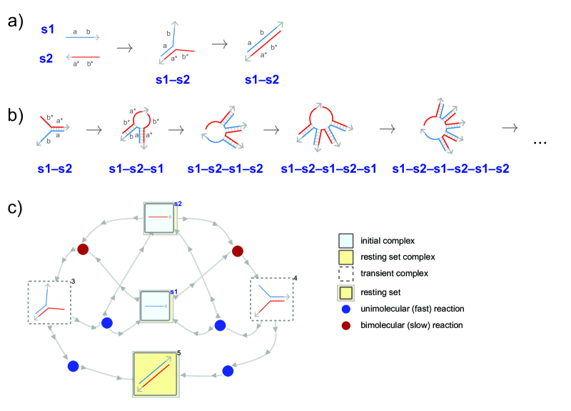
Figure 1: The Polymerization Problem. Reaction enumerators must avoid generation of infinitely-long polymers. (a) Intended behavior for a simple system of two strands. Binding between the red strand and the blue strand results in the formation of a stable duplex (the binding could be nucleated by binding between either domain a/a^* or domain b/b^*—here we show only the former for simplicity). (b) Pathological behavior in an enumerator without a separation of timescales. Repeated bimolecular association reactions are allowed to occur before the intramolecular binding reaction, generating implausibly long polymers. Depending on the order in which the enumerator searches for reactions, this could prevent such an enumerator from ever finding the kinetically- and thermodynamically-favored complex—the simple duplex. (c) Reaction network generated by our enumerator. Separation of reactions into “fast” (unimolecular) and “slow” (bimolecular) allows the classification of certain complexes (dashed boxes) as “transients”; by prohibiting the transient complexes from participating in bimolecular reactions, the pathway generated by our enumerator converges on the intended duplex.

A series of inspiring demonstrations during the last 15 years have shown DNA to be a robust and versatile substrate for nanoscale construction and computation^{1, 2, 3, 4}. DNA has been used to build tile assemblies^{5, 6}; arbitrary shapes^{7, 8}; molecular motors^{9, 10, 11}, walkers^{12, 13, 14, 15}, and robots^{16, 17}; analog circuits that perform amplification of concentrations^{18, 14, 19} and polymer lengths^{20, 14}; synthetic transcriptional circuits²¹; molecular logic gates²²; Turing-universal stack machines²³; and application-specific analog and digital circuits that perform non-trivial calculations^{24, 25, 26, 1}. A common abstraction is to describe these complex systems in terms of a number of “domains”—contiguous sequences of nucleotides that are intended to participate in hybridization as a group; complementary domains are intended to interact, and all other domains are not. Once a system has been described in terms of domains, a computational sequence design package can generate a sequence of nucleotides for each domain in the system, implementing the desired complementarity rules^{27, 28}. Developing such increasingly complex dynamic DNA nanosystems requires tools both for the automated design of these systems, but also for software-assisted verification of their behavior^{29, 30}.

One mode of verification is to check whether a set of DNA complexes can react to produce the desired product species (or various anticipated intermediate species). Given a domain-level model, this can be done by enumerating the network of all possible reactions that can occur, starting from a finite set of initial complexes. The result is a chemical reaction network (equivalently a Petri net), connecting these initial complexes to some set of intermediate complexes. For the sake of this paper, we use the term “enumeration” to refer to the process of generating a chemical reaction network, given a set of initial complexes and a set of rules for their possible interactions.

This enumeration process, by itself, does not fully describe the expected kinetic behavior of the system, because the concentration (or number of copies) of each initial species is not yet specified. However, the enumerated network of reactions forms the basis of a system’s dynamics, and therefore a great deal can often be observed about a system’s behavior simply by examining the network of reactions. Unintended side reactions that could hamper the kinetics of the system or cause unanticipated failure modes can be identified. Furthermore, given initial concentrations (or counts), the chemical reaction network can be simulated using deterministic ordinary differential equations (ODEs) or stochastic methods, and in some cases global properties of the dynamics can be analyzed. In dynamic DNA nanotechnology, this type of enumeration, like the design, has often been performed by hand; this is clearly infeasible for all but the most simple systems, as the number of possible unintended interactions between two species grows quadratically in the number of domains. Worse, the combinatorial structure inherent in the rearrangement and assembly of strands can give rise to an exponential—potentially even infinite—number of species. Thus, automated methods for performing the enumeration are essential, and for tractability it is necessary that they focus attention on only the most relevant possible complexes and reactions. Rule-based models developed for concisely representing combinatorial structures in systems biology, such as BioNetGen³¹ or Kappa³², could in principle be used for DNA systems, but appropriate rules for the relevant DNA interactions would have to be provided by the user for each system.

Several previous efforts have explored the in silico testing and verification of dynamic DNA nanotechnology systems using a built-in set of rules. Most notably, Phillips and Cardelli have demonstrated the DNA circuit compiler and analysis tool “Visual DSD,” which was subsequently extended by Lakin et al.^{29, 33, 34} The analysis component of DSD allows for enumeration of possible reactions between a set of initial complexes, and then simulation of those reactions—either using a system of ODEs or a stochastic simulation. DSD also allows a hybrid “just-in-time” enumeration model which interleaves enumeration with simulation; in this model, reactions are stochastically selected for pursuit by the enumerator based on their estimated probabilities (rather than the entire network being enumerated exhaustively) . However, DSD has a limited system of representation for strand displacement systems; in particular, the formalism cannot represent branched junction, hairpin, or multiloop structures. Similarly, the DSD model cannot currently express reactions relying on looped or branched intermediates, such as 4-way branch migration or remote toehold-mediated 3-way branch migration³⁵. These structural motifs and reaction mechanisms have proven useful in recent experimental work for self-assembly^{14, 36}, locomotion^{11, 17}, imaging³⁷, and computation. Earlier work by Nishikawa et al. included a similar joint enumeration and simulation model that allows arbitrary secondary structures using strands with “abstract bases” analogous to our “domains”; combinatorial explosion was controlled by only allowing interactions between complexes above some threshold concentration³⁸. More recent work by Kawamata et al. uses a graph-based model to represent and simulate reactions between species^{39, 40}.

Here, our goal was to develop a domain-level reaction enumerator that (a) separates the enumeration and simulation steps so that the resulting reaction network can be rigorously analyzed, (b) models a wide range secondary structures and conformational mechanisms used in dynamic DNA nanotechnology, and (c) controls combinatorial explosion using an approximation that is valid in a well-defined limit, thus allowing simplification of the resulting network. Our enumerator, which we call Peppercorn, exhaustively determines the possible hybridization reactions between a set of initial complexes, as well as between any complexes generated as products of these reactions, yielding a complete reaction network. The enumerator can represent arbitrary non-pseudoknotted complexes, and handles 3-way and 4-way branch migration, including reactions initiated by remote toeholds. It enforces a separation of timescales in order to avoid implausible polymerization that would otherwise result from this degree of generality. Finally, it includes a scheme for “condensing” reactions to consider only slow transitions between groups of species—excluding transient intermediate complexes. We have implemented the Peppercorn enumerator in Python, and it has been included as part of the DyNAMiC Workbench Integrated Development Environment³⁰, which is available online with a graphical user interface (www.molsys.net/workbench).

The driving issue in the development of our enumerator has been the need to model as wide a range of secondary structures as possible. We chose non-pseudoknotted secondary structures, a class that includes not only the linear and “hairy linear” structures of DSD, but also branched tree-like structures with hairpin loops, bulge loops, interior loops, and multiloop junctions (Fig. S3). (Pseudoknotted structures, in which branches of a tree can contact each other to form cycles, require more complicated energy models, have geometrical constraints, and are not extensively used in dynamic DNA nanotechnology yet, so version 1.0 of Peppercorn does not allow them. See Appendix D and Fig. S4 for further explanation.)

The choice to allow arbitrary non-pseudoknotted structures, and arbitrary hybridization interactions between them, introduces some problems that don’t arise in restricted models such as Visual DSD. For example, some sets of species may allow for the generation of infinitely long polymers (Fig. 1); a naive attempt to enumerate all possible reactions in such a system would prevent the algorithm from terminating. In the laboratory, these polymers will not occur at low concentrations if kinetically faster reactions are possible that preclude polymerization. Therefore, the enumerator must provide some plausible approximation for a separation of kinetic timescales. We find here that the low-concentration limit, in which unimolecular reactions are sufficiently faster than bimolecular reactions, provides a clean and rigorous basis for a semantics that avoids the spurious polymerization issue.

Finally, it is desirable that the results of this enumeration be interpretable to the user—an excessively complex reaction network will be useful only for performing kinetic simulations and will make it hard to distinguish intended reaction pathways from unintended side reactions. Simplification may be necessary for further verification (for instance, comparison of the system’s predicted behavior to a specification, given in a higher level language). It is essential that any simplification has some guaranteed correspondence to the full, detailed reaction network. Given a presumed separation of timescales, one way to make the network more interpretable is to show only the “slow” reactions, and to assume that “fast” reactions happen instantaneously. We will explore this idea in detail later.

As a motivating example, we show the 3-arm junction system of Yin et al. in Fig. 2¹⁴; this system involves the assembly of a 3-arm junction from a set of metastable hairpins, triggered by the addition of a catalyst (Fig. 2a). The catalyst opens one hairpin by toehold-mediated branch migration, exposing another toehold (previously sequestered within the hairpin stem); this toehold similarly opens the second hairpin, which can open the third hairpin. In the final step, a four-strand intermediate complex (containing the three hairpins and the initiator) can collapse to the final 3-arm junction structure, releasing the single-strand catalyst. Even for this simple process, the full, detailed reaction network is rather complicated (because of the separate toehold-nucleation steps necessary for attachment of each hairpin to the growing structure, as well as various unintended side reactions). These steps result in transient intermediates that quickly decay to a more stable “resting complex.” By skipping these transient intermediates (and depicting only bimolecular transitions between sets of resting complexes), the reaction network can be greatly simplified (Fig. 2b).

Figure 2: Catalytic 3-arm junction formation. We show the catalytic 3-arm junction assembly process (originally demonstrated by Yin et al. ¹⁴), as enumerated by our software; the intended pathway is highlighted in red and purple. Boxes with rounded edges represent complexes—initial complexes have blue backgrounds, “transient” complexes have dashed borders (e.g. complex 5), and “resting complexes” have yellow backgrounds. Circular nodes are reactions—“unimolecular” (blue) and “bimolecular” (red) reactions. “Resting sets” are shown as light yellow boxes around complexes (in this case, each resting set has only one complex). (a) Detailed reactions. A set of three strands (n2, n3, n4) begin as metastable hairpin monomers. A single-stranded initiator (n1) induces toehold attachment (5) and opening of the first hairpin, exposing a sequestered toehold (11). The opened hairpin-initiator complex can bind the second hairpin (n3) in a similar process, and so on for the third hairpin (n4). Finally, remote toehold-mediated branch migration allows n4 to displace the initiator n1, allowing for multiple turnover. Greyed-out reactions and complexes indicate non-productive binding. (b) Condensed reaction graph, showing only reactions between “resting sets.” (c) Key complexes are shown in detail.

3 Reaction Enumeration Model

3.1 Primitives and Definitions

We begin by defining some terms necessary for a discussion of the reaction enumeration algorithm and process. These terms are also demonstrated in Fig. 2.

Definition 1.

A domain $d=(z,\sigma)$ is a tuple where $z$ is the name of the domain and $\sigma$ is the (optional) string of nucleotides from the alphabet $\Sigma=\left\{A,C,T,G\right\}$. The length of a domain $d$ is written as $|d|$ and represents the number of nucleotides in the sequence $\sigma$. The enumerator semantics depend only on $|d|$ and not on the actual sequence, thus allowing the domain-level dynamics to be specified prior to sequence design. A domain $d=(z,\sigma)$ has a complementary domain $d^{*}$ whose name is generally $z^{*}$ and whose sequence is the Watson-Crick complement of $s$.

Definition 2.

A strand $s=(z,D)$ is a tuple where $z$ is the name of the strand and $D$ is a sequence of domains $\langle d_{1},d_{2},\ldots\rangle$, ordered from the 5’ end of the strand to the 3’ end. Two strands are equal if and only if their names are equal and they contain identical sequences of domains.

Definition 3.

A structure $T=\langle T_{1},T_{2},\ldots T_{n}\rangle$ (for a sequence of $n$ strands) is a sequence of lists of bindings, where each binding is either a pair of integers or $\varnothing$. That is, $T_{i}=\langle T_{i,1},T_{i,2},\ldots\rangle$ is the structure for strand $i$. $T_{i,j}=(s_{i,j},d_{i,j})$ is a tuple indicating that domain number j within strand number i is bound to domain number $d_{i,j}$ in strand number $s_{i,j}$. This encoding is redundant because $T_{i,j}=(i^{\prime},j^{\prime})\iff T_{i^{\prime},j^{\prime}}=(i,j)$. If a domain is unbound, $T_{i,j}=\varnothing$.

Definition 4.

A complex $c=(z,S,T)$ is a tuple where $z$ is the name, $S$ is the sequence of strands in the complex, and $T$ is the structure of the complex.

• A complex can be rotated by circularly permuting the elements of $S$ and $T$ (e.g. $S^{\prime}=\langle S_{n},S_{1},S_{2},\ldots,S_{n-1}\rangle$) and setting $s_{i,j}=1+((s_{i,j}+n-1)\mod n)$ for all $s_{i,j}\in T_{i}$ for all $T_{i}\in T$). Note that for a non-pseudoknotted complex, the sequence of strands has a unique circular ordering in which the base pairs are properly nested, but there are multiple equivalent circular permutations of the complex⁴¹. Therefore we say the resulting complex is in canonical form if the lexicographically (by the strand name) lowest strand $S_{\ell}$ appears first (e.g. $S_{1}=S_{\ell}$). A complex may be rotated repeatedly in order to achieve canonical form. Two complexes in canonical form are equal if they contain the same strands in the same order, and their structures are equal.

• A complex must be “connected”, which means that all strands in the complex are connected to one another. Two strands $S_{1}$ and $S_{2}$ are “connected” if either $S_{1}$ is bound to $S_{2}$ or $S_{1}$ is bound to some other strand that is connected to $S_{2}$.

Definition 5.

A reaction $r=(A,B)$ is a tuple where $A$ is the multiset of reactants and $B$ is the multiset of products, where reactants and products are both complexes. We write $\rho(r)$ to represent the rate of $r$.

• The arity $\alpha(r)$ of a reaction $r$ is a pair $(|A|,|B|)$, where $|A|$ counts the total number of elements in $A$, and similarly for $|B|$. Any reaction with arity $(1,n)$ is unimolecular; reactions with arity $(2,n)$ are bimolecular, and those with other arities are higher order. For the sake of this paper, we do not consider $(0,n)$ or $(n,0)$ reactions (those which birth new products from no reactants or cause all reactants to disappear).

• A reaction may be classified as fast or slow; we make this separation based on the arity of the reaction (unimolecular reactions are fast, while bimolecular and higher-order reactions are slow). This assumption is rooted in the Law of Mass Action for chemical kinetics. For a unimolecular reaction $A\to B$, the rate $\rho_{\text{uni}}$ of the reaction is given by $\rho_{\text{uni}}=k_{\text{uni}}[A]$ where $[A]$ is the concentration of species $A$, and $k_{\text{uni}}$ is a rate constant. For a bimolecular reaction $A+B\to C$, the rate $\rho_{\text{bi}}$ of the reaction is given by $\rho_{\text{bi}}=k_{\text{bi}}[A][B]$, where $[A]$ is the concentration of species $A$, $[B]$ is the concentration of $B$, and $k_{\text{bi}}$ is a rate constant.

  This means that, as the concentration of all species decreases, the rates of bimolecular reactions decreases more quickly than the rates of unimolecular reactions. Intuitively, this is because bimolecular reactions require the increasingly improbable collision of two species (rather than one species simply achieving sufficient transition energy). Therefore, the assumption of a “clean” separation of timescales (such that all unimolecular reactions occur at a faster rate than any bimolecular reactions) is only valid at sufficiently low concentrations.

• For a set $R$ of reactions, we sometimes write $R_{f}$ to represent the fast reactions and $R_{s}$ to represent the slow reactions, such that $R=R_{f}\cup R_{s}$. Finally, it will be sometimes useful to partition $R_{f}$ into $(1,1)$ and $(1,n)$ reactions, such that $R_{f}=R_{f}^{(1,1)}\cup R_{f}^{(1,n)}$, where by convention $n>1$.

Definition 6.

A resting set $Q$ is a set of one or more complexes—strongly-connected by fast (1,1) reactions—with no outgoing fast reactions of any arity. That is, fast reactions can interconvert between any of the complexes within $Q$, but no fast reaction is possible that transforms a complex in $Q$ to any complex outside of $Q$. We write this as: $\forall r=(A,B)\in R_{f}:A\subseteq Q\rightarrow B\subseteq Q$.

• Complexes which belong to resting sets are called resting complexes; all other complexes are transient complexes.

Definition 7.

A reaction network is a pair $G=(C,R)$ where $C$ is a set of species (either complexes or resting sets) and $R$ is a set of reactions between those species.

• When $C$ is a set of complexes, we refer to $G$ as a “detailed reaction network.” In Sec. 5 we discuss reaction networks where $C$ is a set of resting sets; these are “condensed reaction networks.”

• Although we may informally refer to a reaction network as a “reaction graph,” the presence of bimolecular reactions means that most reaction networks cannot be simply represented as a graph whose vertices are complexes and whose reactions are edges.

  If $R$ contains only $(1,1)$ reactions, than we can consider $G$ to be a directed graph, where $C$ are the vertices, and each reaction $r=(\left\{a\right\},\left\{b\right\})\in R$ is an edge connecting the reactant complex $a$ to the product complex $b$. We use this representation to define a notion of resting sets (above), and to provide a scheme for condensing a reaction network.

  Alternatively, a reaction network may be represented as bipartite graph $G^{\prime}=(V,E)$, where the set of vertices $V=C\cup R$, and the edges in $E$ are pairs $(c,r)$ or $(r,c)$ for some $r\in R$, $c\in C$. For instance, this would allow a reaction $r$ such as:

  $$X+Y\to Z$$

  to be represented by the graph $G=(\left\{X,Y,Z\right\}\cup\left\{r\right\},\left\{(X,r),(Y,r),(r,Z)\right\})$. We use this representation only when visually depicting reaction networks, as in Fig. 2. In all other cases in this paper, the graphs we refer to will be unipartite where the vertices are species.

Definition 8.

A “reaction enumerator” is therefore a function which maps a set of complexes $\mathcal{C}$ to a set of reactions $\mathcal{R}$ between those complexes. Therefore application of a reaction enumerator to a set of complexes yields a reaction network.

We note briefly that these notions are related to other models of parallel computing, particularly Petri nets ^{42, 43}. Our reaction networks could also be considered Petri nets, where the species (either complexes—for a detailed reaction network, or resting sets—for a condensed reaction network) are “places” and the reactions are “transitions.” In a test tube, there would be a finite number of molecules for each individual species—in the language of Petri nets, molecules are called “tokens”, and a “marking” is an assignment of token counts (molecule numbers) to each place (species).

We emphasize that the “enumeration” task at hand is determination of the CRN/net itself—we are not enumerating possible molecule counts/markings of the net. Rather, we assume a finite initial set of complexes and—given some rules about how those complexes may interact—attempt to list all possible reactions that may occur. In the next section, we describe these interaction rules.

3.2 Reaction types

The enumerator relies on the definition of several “move functions”—a move function takes a complex or set of complexes and generates all possible reactions of a given type. In principle, many reaction types are possible; however, we restrict ourselves to the following four basic types, further classifying each type by arity. Here we provide the move functions for each of these reaction types. The different reaction types are summarized in Fig. 3.

Note: when clear from context which complex is under consideration, we will sometimes write $d_{i,j}$ to refer to domain $d_{j}$ on strand $s_{i}$ in this complex. Similarly, if $X=(i,j)$, we may write $d_{X}$ to refer to $d_{i,j}$.

Binding

– two complementary, unpaired domains hybridize to form a new complex (Fig. 3a).

• (1,1) binding – binding occurs between two domains in the same complex. These reactions can be discovered by traversing each domain on each strand and looking ahead for higher-indexed domains that are complementary (within a multiloop, skipping over stems that lead to branched structures, in order to avoid generating pseudoknots); a separate reaction is generated for each separate complementary pair. See Alg. S1 for pseudocode.

• (2,1) binding – binding occurs between two domains on different complexes. These reactions can be found by comparing each domain in one complex $c$ to each domain in another complex $c^{\prime}$, generating a separate reaction to join each complementary pair that is found. See Alg. S2 in the apppendix for pseudocode.

Opening

– two paired domains in a complex detach (Fig. 3b). We assume that there is some threshold length $L$, such that duplexes less than or equal to $L$ nucleotides long can detach rapidly (in unimolecular fast reactions), while domains longer than $L$ bind irreversibly. $L$ is a parameter that can be set by the user; the default value is $L=8$.

These reactions can be found by examining each domain $d_{j}$ on a complex that is bound to a higher-indexed domain, looking to the left and right of that domain (along the same strand) to determine the total length $\ell$ in nucleotides of the helix containing $d_{j}$. If $\ell<L$, a new reaction is generated that detaches all bound domains in the helix. See Alg. S3 in the appendix for pseudocode.

• (1,1) opening – two paired domains in a complex detach, but the complex remains connected

• (1,2) opening – two paired domains in a complex detach, and the complex dissociates into two complexes

3-way

– an unpaired domain replaces one domain in a nearby duplex (branch migration) (Fig. 3c). These reactions can be discovered as follows: for each bound domain with an adjacent unbound domain on each strand (the invading domain), look first to the left and then to the right of that domain—skipping over internal loops—for a third bound domain (the displaced domain) that is complementary to the invading domain. If the displaced domain is directly adjacent to the bound domain (on the same strand), then this is “direct toehold-mediated branch migration”; otherwise (e.g. if the bound domain and the displaced domain are separated by an internal loop), this is known as “remote toehold-mediated branch migration.”³⁵ See Alg. S4 in the appendix for pseudocode.

• (1,1) 3-way – the branch migration results in a complex which remains connected

• (1,2) 3-way – the branch migration releases a complex

4-way

– a four-arm junction is re-arranged such that hybridization is exchanged between several strands (Fig. 3d). See Alg. S5 in the appendix for pseudocode.

• (1,1) 4-way – the branch migration results in a complex which remains connected

• (1,2) 4-way – the branch migration releases a complex

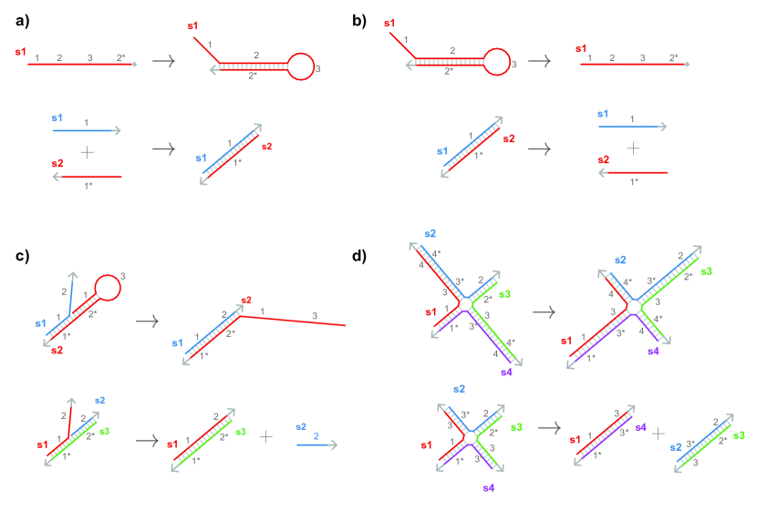
Figure 3: Available reaction types. (a) Bind (1,1) and (2,1). (b) Open (1,1) and (1,2). (c) 3-way branch migration (1,1) and (1,2). (d) 4-way branch migration (1,1) and (1,2)

3.3 Separation of timescales

Reactions are classified as fast or slow according to their arity; as discussed above ($1,n$) reactions are fast for all $n\geq 0$, while all other reactions are slow. Complexes are partitioned into “transient complexes” and “resting complexes.” Resting complexes are those complexes that are part of a “resting set”, while transient complexes are all other complexes. resting sets are calculated as follows: consider a reaction network $C,R$; we can construct a graph $G=(C,R_{f}^{(1,1)})$ where $R_{f}^{(1,1)}$ is the set of fast $(1,1)$ reactions in the reaction network. We compute the set $W$ of “strongly-connected components” of $G$; Each component $W_{i}\in W$ is a resting set if and only if there are no outgoing fast reactions for any complex in $W_{i}$. That is, for some resting set $Q\in W$, any fast reaction consuming a complex in $Q$ produces only products that are in $Q$.

Intuitively, resting sets are sets of complexes that can interconvert rapidly between one another, whereas transient complexes are those which (via only fast reactions) rapidly react to become different complexes (eventually resting complexes). Given infinite time, all molecules that begin in transient complexes will eventually reach a resting set, and all complexes within a resting set will be visited infinitely often by any molecule that remains in the resting set.

Our assumption of a separation of timescales allows the following simplification to be made—transient complexes are unlikely to undergo slower bimolecular (or higher-order) reactions, since fast reactions rapidly transform them to other complexes. We therefore assume that only resting complexes can participate in slow reactions. This simplification avoids consideration of a large number of highly unlikely reaction pathways and intermediate complexes. For instance, it significantly reduces the problem of potentially infinite polymerization, as shown in Fig. 1b. Similarly, consider the example of the three-arm junction (Fig. 2). Before the junction closes, displacing the initiator, it is possible for another hairpin to bind the exposed third-arm, catalyzing the formation of a fourth arm; this process could repeat, creating an implausibly large polymeric structure. We recognize that, in the limit of low concentrations, the bimolecular association will be much slower than the unimolecular branch migration. By classifying the intermediate complex as transient (to be quickly resolved by the formation of a completed 3-arm junction), we prohibit the bimolecular association reaction that could result in the polymer. Additionally, since the enumeration of unimolecular reactions is linear in the number of species, while enumeration of bimolecular reactions is quadratic, eliminating the consideration of bimolecular reactions between transient complexes effectively reduces the complexity of the enumeration problem.

It should be noted that the set of reactions presented in our model still does not describe all possible behaviors of DNA strands—notably, “partial” binding between domains is not possible, and none of the reactions produces complexes that are pseudoknotted. Additional details are provided in the appendix.

4 Reaction Enumeration Algorithm

The essence of the reaction enumeration algorithm is as follows:

1. Exhaustively enumerate complexes reachable from the initial complexes by fast reactions.

2. Classify those complexes into transient complexes or resting complexes (by calculating the SCCs in terms of fast reactions and marking those SCCs with no outgoing fast reactions resting sets).

3. Enumerate slow (bimolecular) reactions between resting complexes.

4. Repeat this process for any new complexes generated by slow (bimolecular) reactions.

Additional details of the algorithm are provided in Sec. A.

5 Condensing reactions

It may not always be desirable or efficient to view—or even to simulate—the entire reaction space, including all transient complexes and individual binding/unbinding events. For this reason, we provide a mechanism of systematically summarizing, or “condensing” the full network of complexes and reactions. In this condensed representation, we represent “transitions” between resting sets as a set of “condensed reactions,” where the reactants and products of condensed reactions are resting sets, rather than individual complexes. Recall that a resting set is a set of one or more complexes, connected by fast reactions (and with no outgoing fast reactions). All of these condensed reactions will be bimolecular. Intuitively, if we assume that fast reactions are arbitrarily fast, then looking only at the resting sets, the condensed reactions will behave exactly the same as the full reaction network. We formalize the correspondance between trajectories in the detailed and the condensed reaction networks in Sec. B.

We define the “condensed reaction network” to be the reaction network $\hat{G}=(\mathcal{Q},\hat{\mathcal{R}})$, where $\mathcal{Q}$ is the set of resting sets and $\hat{\mathcal{R}}$ is the set of condensed reactions. For clarity, we will refer to the “full”, non-condensed reaction network $G=(\mathcal{C},\mathcal{R})$ as the “detailed reaction network”. The goal of this section, therefore, is to describe how to calculate the condensed reaction network $\hat{G}$ from the detailed reaction network $G$. We later prove some properties of this transformation—namely that transitions are preserved between the two reaction networks in Sec. B.

Since much of the following discussion will involve both sets (which may contain only one instance of each member), and multisets (which may contain many instances of any element—for example, the reactants and products of a chemical reaction are each multisets), we will use blackboard-bold braces $\BeginAccSupp{method=hex,unicode,ActualText=2983}\textnormal{\char 102\relax}\mathchoice{\mkern-4.05mu}{\mkern-4.05mu}{\mkern-4.3mu}{\mkern-4.8mu}\textnormal{\char 106\relax}\EndAccSupp{}~{}\BeginAccSupp{method=hex,unicode,ActualText=2984}\textnormal{\char 106\relax}\mathchoice{\mkern-4.05mu}{\mkern-4.05mu}{\mkern-4.3mu}{\mkern-4.8mu}\textnormal{\char 103\relax}\EndAccSupp{}$ to represent multisets and normal braces $\left\{~{}\right\}$ to represent sets. Let us also define a useful operation on sets of multisets. Let $A$ and $B$ be sets of multisets; then we will define the “Cartesian sum” of $A$ and $B$ to be $A\oplus B=\left\{a+b:a\in A,b\in B\right\}$. . It is easily shown that the Cartesian sum is associative and commutative. We will therefore also sometimes write $\bigoplus_{b_{i}\in B}b_{i}$ to represent $b_{1}\oplus b_{2}\oplus\ldots$ for all $b_{i}\in B$.

We will attempt to present this section as a self-contained theory about condensed reaction networks that will be independent of the particular details of the detailed reaction enumeration algorithm. However, we will make certain restrictions on the detailed reaction network to which this algorithm is applied. The reader can verify that the reaction enumeration algorithm presented above satisfies these properties, even when the enumeration terminates prematurely (as in Sec. A.1):

1. All fast reactions are unimolecular, and all slow reactions are bimolecular or higher order.

2. Reactions can have any arity $(n,m)$, as long as $0<n\leq 2$ and $m>0$.

3. For any sequence of unimolecular reactions, where each reaction consumes a product of the previous reaction and the last reaction produces the original species, the sequence must consist only of 1-1 reactions.

4. Reactants of non-unimolecular reactions must be resting complexes.

Fig. 4 provides an example of the reaction condensation process. Before we explain this process, let us clarify a few properties of the detailed reaction network, based on our definitions. Considering the detailed reaction network $G=(\mathcal{C},\mathcal{R}_{f}\cup\mathcal{R}_{s})$, let $\mathcal{R}_{f}^{(1,1)}$ be the fast (1,1) reactions in $\mathcal{R}$. First note that the complexes in $\mathcal{C}$ and the fast reactions $\mathcal{R}_{f}^{(1,1)}$ form a directed graph $\Gamma=(\mathcal{C},\mathcal{R}_{f}^{(1,1)})$. We will be calculating the strongly-connected components (SCCs) of this graph using Tarjan’s algorithm, as we did in the reaction enumeration algorithm. Note that every complex (whether a resting complex or a transient complex) is a member of some SCC of $\Gamma$. Let us denote by $\mathbb{S}(x)$ the SCC of $\Gamma$ containing some complex $x$. The resting sets of $G$ are the SCCs for which there are no outgoing fast reactions of any arity. There may be (even large) SCCs that only contain transient complexes, because there is at least one outgoing fast reaction from the SCC; for instance, in Fig. 4, $\left\{1,2\right\}$ is an SCC, but is not a resting set (because of the fast reaction $2\to 3$). Also note that many SCCs may contain only one element (for instance, $\left\{3\right\}$ is an SCC). Finally, observe that we can form another graph, $\Gamma^{\prime}$, where the nodes are SCCs of $\Gamma$, and there is a directed edge between SCCs if there is a $(1,m)$ reaction with a reactant in one SCC and a product in the other. That is, $\Gamma^{\prime}=(S,E)$ where $E=\left\{S(a),S(b_{i})\forall b_{i}\in B:r=(\BeginAccSupp{method=hex,unicode,ActualText=2983}\textnormal{\char 102\relax}\mathchoice{\mkern-4.05mu}{\mkern-4.05mu}{\mkern-4.3mu}{\mkern-4.8mu}\textnormal{\char 106\relax}\EndAccSupp{}a\BeginAccSupp{method=hex,unicode,ActualText=2984}\textnormal{\char 106\relax}\mathchoice{\mkern-4.05mu}{\mkern-4.05mu}{\mkern-4.3mu}{\mkern-4.8mu}\textnormal{\char 103\relax}\EndAccSupp{},B)\in R_{o}\wedge\alpha(r)=(1,m)\right\}$. $\Gamma^{\prime}$ is a directed acyclic graph (since all cycles were captured by the SCCs). The leaves of $\Gamma^{\prime}$ (those vertices with no outgoing edges) are the resting sets of $G$.

Definition 9.

A “fate” $F$ of a complex $x$ is a multiset of possible resting sets, reachable from $x$ by fast reactions.

$F$ is a multiset because, for instance, $x$ may be a dimer that can decompose into two identical complexes, both of which are resting complexes, such that: $x\rightarrow y+y$. Any complex $x$ may have many such fates, and all complexes must have at least one fate. We will denote the set of such fates by $\mathbb{F}(x)$. Computing $\mathbb{F}(x)$ for all complexes $x$ in the ensemble therefore allows each complex to be mapped to a set of possible resting set fates. More generally, we may think about the fate of a multiset of complexes; this answers the question “to what combinations of resting sets can some molecules evolve, starting in this multiset of complexes, exclusively via fast reactions?” Let us define $\mathbb{F}(X)$ where $X=\BeginAccSupp{method=hex,unicode,ActualText=2983}\textnormal{\char 102\relax}\mathchoice{\mkern-4.05mu}{\mkern-4.05mu}{\mkern-4.3mu}{\mkern-4.8mu}\textnormal{\char 106\relax}\EndAccSupp{}x_{1},x_{2},\ldots\BeginAccSupp{method=hex,unicode,ActualText=2984}\textnormal{\char 106\relax}\mathchoice{\mkern-4.05mu}{\mkern-4.05mu}{\mkern-4.3mu}{\mkern-4.8mu}\textnormal{\char 103\relax}\EndAccSupp{}$ to be:

$$\mathbb{F}(X)=\bigoplus_{x\in X}\mathbb{F}(x)=\mathbb{F}(x_{1})\oplus\mathbb{F}(x_{2})\oplus\ldots$$

The intuition is that, since fates for different complexes are independent, the set of possible fates of $X$ is the set of all possible combinations of the fates of $x_{1}$, $x_{2}$, etc. From here, we can define the related notion for some reaction $r=(A,B)$, where $B=\BeginAccSupp{method=hex,unicode,ActualText=2983}\textnormal{\char 102\relax}\mathchoice{\mkern-4.05mu}{\mkern-4.05mu}{\mkern-4.3mu}{\mkern-4.8mu}\textnormal{\char 106\relax}\EndAccSupp{}b_{1},b_{2},\ldots b_{n}\BeginAccSupp{method=hex,unicode,ActualText=2984}\textnormal{\char 106\relax}\mathchoice{\mkern-4.05mu}{\mkern-4.05mu}{\mkern-4.3mu}{\mkern-4.8mu}\textnormal{\char 103\relax}\EndAccSupp{}$. Let $\mathbb{R}(r)=\mathbb{F}(B)$, such that:

$$\mathbb{R}(r)=\mathbb{F}(B)=\bigoplus_{b\in B}\mathbb{F}(b)=\mathbb{F}(b_{1})\oplus\mathbb{F}(b_{2})\oplus\ldots\oplus\mathbb{F}(b_{n}).$$

Finally, let $R_{o}(S)$ be the set of reactions leaving some SCC $S$ of $\Gamma$.

With these definition, we can provide an expression for $\mathbb{F}(x)$ in terms of a recursion:

$$\mathbb{F}(x)=\begin{cases}\left\{\mathbb{S}(x)\right\}&\text{if }\mathbb{S}(x)\text{is a resting set}\\ \bigcup_{r\in R_{o}\left(\mathbb{S}(X)\right)}\mathbb{R}(r)&\text{otherwise}\\ \end{cases}$$ (1)

The “base case” is that, if $x$ is a resting complex, then $\mathbb{F}(x)$ is just $x$’s resting set. The recursive case can be evaluated in finite time, because $\Gamma^{\prime}$ is a directed acyclic graph. That is, if we start with some arbitrary transient complex $x$, the recursion can be evaluated by a depth-first traversal of $\Gamma^{\prime}$, starting from $x$; since $\Gamma^{\prime}$ is acyclic, each branch of the depth-first traversal will terminate at a leaf of $\Gamma^{\prime}$—a resting complex for which $\mathbb{F}(x)$ is trivial.

Once we have computed $\mathbb{F}(x)$, we can easily calculate the set of condensed reactions. Since $\mathbb{F}(x)$ captures all of the information about the fast reactions in which $x$ participates, we must only consider slow reactions. For each slow reaction $s=(A,B)$ in the detailed reaction network, where $A$ is the multiset of reactant complexes and $B$ is the multiset of product complexes, we will generate some number of condensed reactions—one for each fate of $B$. Specifically, the condensed reaction network $\hat{G}=(\hat{C},\hat{R})$ has $\hat{C}$ being the set of resting sets; we build $\hat{R}$ as follows: for each slow reaction $s=(A,B)\in R$, with $\mathbb{S}(A)=\BeginAccSupp{method=hex,unicode,ActualText=2983}\textnormal{\char 102\relax}\mathchoice{\mkern-4.05mu}{\mkern-4.05mu}{\mkern-4.3mu}{\mkern-4.8mu}\textnormal{\char 106\relax}\EndAccSupp{}\mathbb{S}(a_{i}):a_{i}\in A\BeginAccSupp{method=hex,unicode,ActualText=2984}\textnormal{\char 106\relax}\mathchoice{\mkern-4.05mu}{\mkern-4.05mu}{\mkern-4.3mu}{\mkern-4.8mu}\textnormal{\char 103\relax}\EndAccSupp{}$, then for each $F\in F(s)$, we add a condensed reaction $(\mathbb{S}(A),F)$ to $\hat{R}$. In Alg. S7 we describe precisely how to calculate $\mathbb{F}(x)$, and then how to compute the condensed reactions from $\mathbb{F}(x)$. In Sec. B we present a set of theorems justifying the choice of this algorithm.

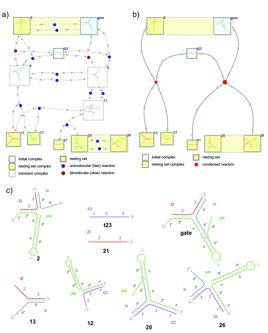
Figure 4: Reaction Condensation Example. In this example, we attempt to illustrate possible complexities in condensing reactions. (a) Detailed reaction network. Beginning with complex gate, rapid interconversion with 2 is possible. Depending on the state of the complex, interaction with t23 yields a variety of breakdown products. (b) Condensed reaction network. The condensed reactions show two possible bimolecular reactions between gate/2 and t23, and that each of these reactions has multiple breakdown products. Although there are two parallel pathways that yield complexes 12 and 13 in the detailed reaction network (via 6 or via 5 and 17), only a single reaction ($\texttt{gate}\to\texttt{13}+\texttt{12}$) appears in the condensed reactions, because the two transient pathways have indistinguishable fates. (c) Key complexes shown in detail.

6 Approximate Kinetics

Thus far we have only discussed the kinetics of the system in the context of our assumption that the timescales for “fast” and “slow” reactions can be separated. We have not addressed the fact that, even within the sets of fast and slow reactions, different reactions may occur at very different rates. Different rates of different reactions can greatly impact the dynamics of the system’s behavior. Therefore in order to make useful predictions about the experimental kinetics of the reaction networks we are studying, we need to consider the rates of these reactions, in addition to simply enumerating the reactions themselves.

In this section, we present a method for approximating the rate laws governing the rates of each of the “move types” discussed in Sec. 3.2, along with an extension for calculating the rates of condensed reactions. Our implementation automatically calculates these rates and includes them in its output, allowing the user to import the resulting model into a kinetic simulator such as COPASI, provide initial concentrations for species, and simulate the resulting dynamics. It is important to emphasize that the rate laws that we provide (in particular, the formulas we give for the rate constants), although based on experimental evidence and intuition, are heuristic and approximate. Also note that the kinetics of a real physical system will be affected by parameters outside the consideration of our model—for instance, the sequences of each domain (and therefore the binding energies) will be different, and the temperature and salt concentrations can both change the energetics of the interactions. These changes can greatly affect the real system’s overall dynamic behavior. The formulas we give here are intended to roughly approximate the rate constants at $25\text{\,}\mathrm{\SIUnitSymbolCelsius}$ and $10\text{\,}\mathrm{m\text{M}}$ Mg²⁺.

Let $\rho(r)$ be the rate of some reaction $r=(A,B)$, where $A={a_{1},a_{2},\ldots}$. For the sake of this section, we will assume that $\rho(r)$ is given by:

$$\rho(r)=k\prod_{a\in A}[a]$$

where $[a]$ represents the concentration of some species $a$, and $k$ a constant, which we call the “rate constant”. Implicit in this choice of rate law is the assumption that all reactions are elementary (meaning there is only a single transition state between the reactants and the products); in reality, this is not the case, as most DNA strand interactions have a complex transition state landscape and involve many intermediate states. Since the enumerator has no knowledge of the concentrations of any species, the problem of estimating the rate $\rho(r)$ of the reaction boils down to estimating the rate constant $k$. We will therefore attempt to provide formulas for approximating these rate constants, such that the overall reaction rates are consistent with experimental evidence in a reasonable concentration regime (sufficiently below micromolar concentrations).

In Sec. C, we provide approximate formulas for the rate constant $k$, for each of the reaction types described above.

6.1 Approximate condensed reaction kinetics

Consider some reaction $\hat{r}=(\hat{A},\hat{B})$ where $\hat{A}=\BeginAccSupp{method=hex,unicode,ActualText=2983}\textnormal{\char 102\relax}\mathchoice{\mkern-4.05mu}{\mkern-4.05mu}{\mkern-4.3mu}{\mkern-4.8mu}\textnormal{\char 106\relax}\EndAccSupp{}\hat{A}_{1},\hat{A}_{2},\ldots\BeginAccSupp{method=hex,unicode,ActualText=2984}\textnormal{\char 106\relax}\mathchoice{\mkern-4.05mu}{\mkern-4.05mu}{\mkern-4.3mu}{\mkern-4.8mu}\textnormal{\char 103\relax}\EndAccSupp{}$ and $\hat{B}$ are multisets of resting sets. Assume $\hat{r}$ is part of a condensed reaction network $(\mathcal{\hat{C}},\mathcal{\hat{R}})$, and that there is a detailed reaction network $(\mathcal{C},\mathcal{R})$. Let $R_{\hat{A}}$ be the set of all detailed bimolecular reactions in $\mathcal{R}$ between representations of $\hat{A}$:

$$R_{\hat{A}}=\left\{r=(A^{\prime},B^{\prime}):r\in\mathcal{R},A^{\prime}\text{ is a representation of }\hat{A}\right\}.$$

For bimolecular reactions (where $\hat{A}=(\hat{A}_{1},\hat{A}_{2})$), then $R_{\hat{A}}$ is given by:

$$R_{\hat{A}}=\left\{r=(\BeginAccSupp{method=hex,unicode,ActualText=2983}\textnormal{\char 102\relax}\mathchoice{\mkern-4.05mu}{\mkern-4.05mu}{\mkern-4.3mu}{\mkern-4.8mu}\textnormal{\char 106\relax}\EndAccSupp{}A^{\prime}_{1},A^{\prime}_{2}\BeginAccSupp{method=hex,unicode,ActualText=2984}\textnormal{\char 106\relax}\mathchoice{\mkern-4.05mu}{\mkern-4.05mu}{\mkern-4.3mu}{\mkern-4.8mu}\textnormal{\char 103\relax}\EndAccSupp{},B^{\prime}):r\in\mathcal{R},A^{\prime}_{1}\in\hat{A}_{1},A^{\prime}_{2}\in\hat{A}_{2}\right\}.$$

The rate law $\rho(\hat{r})$ for the condensed reaction $\hat{r}$ will be given by:

$$\rho(\hat{r})=k\prod_{\hat{A}_{i}\in\hat{A}}[\hat{A}_{i}]$$

where $[\hat{A}_{i}]$ represents the concentration of the resting set $\hat{A}_{i}$, which we can assume to be in equilibrium relative to the fast reactions. We can consider $[\hat{A}_{i}]$ to be the sum over the concentrations of the species in $\hat{A}_{i}$:

$$[\hat{A}_{i}]=\sum_{a\in\hat{A}_{i}}[a].$$

Again, the real challenge will be predicting the rate constant $k$.

For simplicity, we will consider only the bimolecular case, where $\hat{A}=(\hat{A}_{1},\hat{A}_{2})$ (the generalization to higher order reactions is simple). The approximate rate constant $k$ is given by

$$k=\sum_{r=(\BeginAccSupp{method=hex,unicode,ActualText=2983}\textnormal{\char 102\relax}\mathchoice{\mkern-4.05mu}{\mkern-4.05mu}{\mkern-4.3mu}{\mkern-4.8mu}\textnormal{\char 106\relax}\EndAccSupp{}a_{1},a_{2}\BeginAccSupp{method=hex,unicode,ActualText=2984}\textnormal{\char 106\relax}\mathchoice{\mkern-4.05mu}{\mkern-4.05mu}{\mkern-4.3mu}{\mkern-4.8mu}\textnormal{\char 103\relax}\EndAccSupp{},B)\in R_{\hat{A}}}\mathbb{P}\left[a_{1}:\hat{A}_{1}\right]\cdot\mathbb{P}\left[a_{2}:\hat{A}_{2}\right]\cdot k_{r}\cdot\mathbb{P}\left[T_{B\to\hat{B}}\right]$$ (2)

where: $\mathbb{P}\left[a_{1}:\hat{A}_{1}\right]$ represents the probability that, at any given time, a single complex in the resting set $\hat{A}_{1}$ will be $a_{1}$, $\mathbb{P}\left[a_{2}:\hat{A}_{2}\right]$ represents the probability that, at any given time, a single complex in the resting set $\hat{A}_{2}$ will be $a_{2}$, $k_{r}$ represents the rate constant for the detailed reaction $r$, as calculated in the previous section, and $\mathbb{P}\left[T_{B\to\hat{B}}\right]$ represents the probability that the complexes in $B$ decay to complexes that represent $\hat{B}$. Note that, if $r$ produces products which can never be converted to the resting sets in $\hat{B}$, then this term will be 0.

The sum is over all reactions which can represent the reactants—that is, we need to consider all possible reactions that can consume one complex from each resting set in $\hat{A}$. The overall rate for the condensed reaction will be proportional to the rates of those detailed reactions, weighted by the joint probability that those reactants are actually present, and that the products decay to the correct resting set.

To calculate $\mathbb{P}\left[a_{1}:\hat{A}_{1}\right]$, $\mathbb{P}\left[a_{2}:\hat{A}_{2}\right]$, and $\mathbb{P}\left[T_{B\to\hat{B}}\right]$, it is helpful to think of each of the SCCs of the the graph $\Gamma$ of the detailed reaction network as individual, irreducible Continuous Time Markov Chains (CTMCs). We will use the results for resting sets to calculate $\mathbb{P}\left[a_{1}:\hat{A}_{1}\right]$, $\mathbb{P}\left[a_{2}:\hat{A}_{2}\right]$, and results for SCCs of transient complexes to derive $\mathbb{P}\left[T_{B\to\hat{B}}\right]$.

Consider first the resting sets. We can treat a single instance of the resting set $A=\left\{a_{1},a_{2},\ldots a_{L}\right\}$ to be a Markov process, periodically transitioning between each of the $L$ states, according to the reactions connecting the various complexes $a_{1},a_{2},\ldots$ in the resting set. We can describe the dynamics of this process by a matrix $\mathbf{T}\in\mathbb{R}^{L\times L}$, where the elements $T_{ij}$ of the matrix represent the rate (possibly zero) of the reaction from state $j$ to state $i$, which we denote $\rho(j\to i)$, and each diagonal element is the negative sum of the column:

$$T_{ij}=\begin{cases}\rho(j\to i)&i\neq j\\ -\sum_{j=1,j\neq i}^{L}T_{ji}&i=j\\ \end{cases}$$ (3)

Let $\mathbf{s}(t)=(s_{1},s_{2},\ldots)^{T}$ be an $L$-dimensional vector giving the probabilities, at time $t$, of being in any of the $L$ states. The continuous-time dynamics of this process obeys

$$\frac{d\mathbf{s}}{dt}=\mathbf{T}\mathbf{s}(t).$$

For a resting set, we assume that the system has reached equilibrium, and so $\mathbf{s}$ is not changing with time. We therefore find the “stationary distribution” $\hat{\mathbf{s}}$ of this process by setting $d\mathbf{s}/dt=0$, and recognizing that $\hat{\mathbf{s}}$ is the right-eigenvector of $\mathbf{T}$ with eigenvalue zero. Given the stationary distribution $\hat{\mathbf{s}}=(\hat{s}_{1},\hat{s}_{2},\ldots,\hat{s}_{L})^{T}$, we recognize that

$$\mathbb{P}\left[a_{i}:A_{i}\right]=\hat{s}_{i}.$$ (4)

Next consider the transient SCCs. To figure the probability $\mathbb{P}\left[T_{B\to\hat{B}}\right]$ that complexes in $B$ decay to complexes that represent $\hat{B}$, we will again model the SCC as a Markov process, but we cannot use the stationary distribution since the transient SCC may be far from equilibrium. Note that this SCC does not represent a resting set, so there are additionally some $e$ outgoing fast reactions that exit the SCC. We will model this SCC, including the outgoing reactions, as an $(L+e)$-state Markov process, where each of the $e$ states is absorbing. We want to know the probability that, having entered the SCC in some state $i\in\left\{1\ldots L\right\}$, it will leave via some reaction $j\in\left\{L+1\ldots L+e\right\}$. We number the reactions in this way to allow them to be discussed consistently as states in the same Markov process as the complexes.

Assume the SCC is again given by $A=\left\{a_{1},a_{2},\ldots a_{L}\right\}$. Let $\mathbf{Q}\in\mathbb{R}^{L\times L}$ be the matrix of transition probabilities within the SCC, such that $Q_{ij}$ is the probability that, at a given time the system’s next transition is from state $i$ to state $j$, where $i,j\in\left\{1\ldots L\right\}$. Let us therefore define an additional matrix $\mathbf{E}\in\mathbb{R}^{L\times e}$, where $E_{ij}$ represents the probability that the system in state $i\in\left\{1\ldots L\right\}$ transitions next to absorbing state $j\in\left\{L+1\ldots L_{e}\right\}$. We define the transition probabilities $Q_{ij}$ and $R_{ij}$ in terms of the transition rates—if $k_{ij}$ is the rate constant of the transition from state $i$ to state $j$, then

$$Q_{ij}=\frac{k_{ij}}{\sum_{j^{\prime}=1}^{L+e}k_{ij^{\prime}}}$$ (5)

and similarly for $R_{ij}$. To calculate the probability of exiting via state $j$ after entering through state $i$, we first define the “fundamental matrix”—which gives the expected number of visits to state $j$, starting from state $i$:

$$\mathbf{N}=\sum_{k=0}^{\infty}\mathbf{Q}^{k}=(\mathbf{I}_{L}-\mathbf{Q})^{-1}$$ (6)

where $\mathbf{I}_{L}$ is the $L\times L$ identity matrix. Let us define the “absorption matrix” $\mathbf{B}=\mathbf{N}\mathbf{R}$; the entries $B_{ij}$ represent the probability of exiting via state $j$ after entering through state $i$.

But what we really need is to calculate the relative probabilities of each of the fates of some complex $x$. Let $\mathbb{P}\left[x\to F\right]$ be the probability that $x$ decays into a given fate $F$.

$$\mathbb{P}\left[x\to F\right]=\begin{cases}1&\text{if $\mathbb{S}(x)$ is a resting set and $\mathbb{F}(x)=\left\{F\right\}$}\\ \sum_{j}{B_{ij}\mathbb{P}\left[r_{j}\to F\right]}&\text{if $\mathbb{S}(x)$ is a transient SCC}\\ 0&\text{if $F\not\in\mathbb{F}(x)$}\end{cases}$$ (7)

where $\mathbf{B}=[B_{ij}]$ is the absorption matrix for $\mathbb{S}(x)$, $i$ represents the index of complex $x$ in $\mathbb{S}(x)$, and $j$ is the index of the reaction exits $\mathbb{S}(x)$, and $\mathbb{P}\left[r_{j}\to F\right]$ is the probability that the products of the reaction $r_{j}$ decay to complexes that represent $F$. More formally, for some reaction $r_{j}=(C,D)$, where $D=\BeginAccSupp{method=hex,unicode,ActualText=2983}\textnormal{\char 102\relax}\mathchoice{\mkern-4.05mu}{\mkern-4.05mu}{\mkern-4.3mu}{\mkern-4.8mu}\textnormal{\char 106\relax}\EndAccSupp{}d_{1},d_{2},\ldots\BeginAccSupp{method=hex,unicode,ActualText=2984}\textnormal{\char 106\relax}\mathchoice{\mkern-4.05mu}{\mkern-4.05mu}{\mkern-4.3mu}{\mkern-4.8mu}\textnormal{\char 103\relax}\EndAccSupp{}$:

$$\mathbb{P}\left[r_{j}\to F\right]=\sum_{\left\{F^{\prime}_{1}+F^{\prime}_{2}+\ldots F^{\prime}_{n}=F\right\}}\mathbb{P}\left[d_{1}\to F^{\prime}_{1}\right]\mathbb{P}\left[d_{2}\to F^{\prime}_{2}\right]\ldots\mathbb{P}\left[d_{n}\to F^{\prime}_{n}\right]$$ (8)

The sum is taken over all of the ways that the fates $\BeginAccSupp{method=hex,unicode,ActualText=2983}\textnormal{\char 102\relax}\mathchoice{\mkern-4.05mu}{\mkern-4.05mu}{\mkern-4.3mu}{\mkern-4.8mu}\textnormal{\char 106\relax}\EndAccSupp{}F^{\prime}_{k}\BeginAccSupp{method=hex,unicode,ActualText=2984}\textnormal{\char 106\relax}\mathchoice{\mkern-4.05mu}{\mkern-4.05mu}{\mkern-4.3mu}{\mkern-4.8mu}\textnormal{\char 103\relax}\EndAccSupp{}\in\BeginAccSupp{method=hex,unicode,ActualText=2983}\textnormal{\char 102\relax}\mathchoice{\mkern-4.05mu}{\mkern-4.05mu}{\mkern-4.3mu}{\mkern-4.8mu}\textnormal{\char 106\relax}\EndAccSupp{}\mathbb{F}(d_{1})\times\mathbb{F}(d_{2})\times\ldots:d_{k}\in D\BeginAccSupp{method=hex,unicode,ActualText=2984}\textnormal{\char 106\relax}\mathchoice{\mkern-4.05mu}{\mkern-4.05mu}{\mkern-4.3mu}{\mkern-4.8mu}\textnormal{\char 103\relax}\EndAccSupp{}$ can combine such that the $\BeginAccSupp{method=hex,unicode,ActualText=2983}\textnormal{\char 102\relax}\mathchoice{\mkern-4.05mu}{\mkern-4.05mu}{\mkern-4.3mu}{\mkern-4.8mu}\textnormal{\char 106\relax}\EndAccSupp{}F^{\prime}_{k}\BeginAccSupp{method=hex,unicode,ActualText=2984}\textnormal{\char 106\relax}\mathchoice{\mkern-4.05mu}{\mkern-4.05mu}{\mkern-4.3mu}{\mkern-4.8mu}\textnormal{\char 103\relax}\EndAccSupp{}$ sum to our target fate $F$ (that is, $\sum_{k}F^{\prime}_{k}=F$. Within the sum, we want to calculate the joint probability that all of the complexes $d_{k}\in D$ decay to their respective fates $F^{\prime}_{k}$. These terms can be computed recursively by Eq. 7.

Finally, we can write an expression for our quantity of interest. We want to know the probability $\mathbb{P}\left[T_{B\to\hat{B}}\right]$; however, we realize now that this can be computed easily using Eq. 8:

$$\mathbb{P}\left[T_{B\to\hat{B}}\right]=\mathbb{P}\left[r\to\hat{B}\right],$$

where $r$ is the original, detailed bimolecular reaction.

Now we have shown how to compute all the terms necessary to evaluate Eq. 2. The structure of our arguments has mirrored the algorithm for deriving the condensed reactions—it is simple to efficiently evaluate Eq. 4, 7, and 8 alongside Alg. S7, and therefore to compute a rate constant $k$ for each condensed reaction.

7 Discussion

We have presented an algorithm for exhaustive enumeration of hybridization reactions between a set of DNA species. Our enumerator is more flexible than previously-presented work, allowing enumeration of essentially all non-pseudoknotted structures; previous enumerators such as Visual DSD have been limited to structures without hairpins or internal loops ³⁴. The imposed separation of timescales allows for general bimolecular reactions to be enumerated without producing a large number of physically implausible reactions and forming a (potentially infinite) polymeric structure. By instead insisting that (at sufficiently low concentrations) all unimolecular reactions will precede bimolecular reactions, we allow unimolecular reactions (for instance, ring-closing or branch migration) to terminate such polymerization reactions. The transient intermediate complex, that could otherwise participate in polymerization, is excluded from consideration of bimolecular reactions.

Further, we have demonstrated a convenient representation for condensing large reaction networks into more compact and interpretable reaction networks. We have proven that this transformation preserves the relevant properties of the detailed reaction network—namely, that all transitions between resting sets are possible in the condensed reaction network—and that the condensed reaction network does not introduce spurious transitions not possible in the detailed reaction network.

Our implementation exhaustively enumerates the full reaction network (or a truncated version of the network if certain trigger conditions are reached). Simulation can then be performed on the full reaction network to determine steady-state or time-course behavior. Visual DSD, includes a “just-in-time” enumeration mode, which combines the enumeration and simulation processes. This algorithm begins with a multiset of initial complexes, and at each step generates a set of possible reactions among those complexes; these possible reactions are selected from probabilistically to generate a new state. In this way, the model produces statistically correct samples from the continuous time Markov chain that represents the time-evolution of the ensemble. This algorithm could be an interesting future extension to our implementation.

Acknowledgements. The authors thank Chris Thachuk, Niles Pierce, Peng Yin, and Justin Werfel for discussion and support. This work was supported by the National Science Foundation grants CCF-1317694 and CCF-0832824 (The Molecular Programming Project).

Appendix A Reaction enumeration algorithm details

The reaction enumeration algorithm works by passing complexes through a progression of several mutable sets; as new complexes are enumerated, they are added to one of these sets, then eventually removed and transferred to a later set. All complexes accumulate in either $\mathcal{T}$ (transient complexes) or $\mathcal{E}$ (resting state complexes). This progression enforces the requirement that each complex be classified as a resting state complex or transient complex, that all fast reactions are enumerated before slow reactions, and that complexes are not enumerated more than once. For simplicity, we assume an operation $\textsc{Pop}(S)$ exists that removes and returns some element from the mutable set $S$.

• $\mathcal{B}$ contains complexes that have had no reactions enumerated yet. Complexes are moved out of $\mathcal{B}$ into $\mathcal{F}$ when their “neighborhood” is considered. We define a “neighborhood” about a complex $c$ to be the set of complexes that can be produced by a series of zero or more fast reactions starting from $c$.

• $\mathcal{F}$ contains complexes in the current neighborhood which have not yet had fast reactions enumerated. These complexes will be moved to $\mathcal{N}$ once their fast reactions have been enumerated.

• $\mathcal{N}$ contains complexes enumerated within the current neighborhood, but that have not yet been characterized as transient or resting states. Each of these complexes is classified, then moved into $\mathcal{S}$ or $\mathcal{T}$.

• $\mathcal{S}$ contains resting state complexes which have not yet had bimolecular reactions with set $\mathcal{E}$ enumerated yet. All self-interactions for these complexes have been enumerated.

• $\mathcal{E}$ contains enumerated resting state complexes. Only cross-reactions with other end states need to be considered for these complexes. These complexes will remain in this list throughout function execution.

• $\mathcal{T}$ contains transient complexes which have had their fast reactions enumerated. These complexes will remain in this list throughout function execution.

Fig. S1 summarizes the progression of complexes through these sets. Additionally, two other sets are accumulated over the course of the enumeration:

• $\mathcal{R}$ contains all reactions that have been enumerated.

• $\mathcal{Q}$ contains all resting states that have been enumerated.

					$\nearrow$	$\mathcal{S}$	$\rightarrow$	$\mathcal{E}$
$\mathcal{B}$	$\rightarrow$	$\mathcal{F}$	$\rightarrow$	$\mathcal{N}$		(no slow reactions enumerated)		(resting state complexes)
					$\searrow$	$\mathcal{T}$
(no reactions enumerated)		(no fast reactions enumerated)		(not classified into transient/resting)		(transient complexes)

Figure S1: Passage of complexes through various lists; complexes begin with no outgoing reactions enumerated ($\mathcal{B}$), then have fast reactions in their neighborhood enumerated ($\mathcal{F}$, $\mathcal{N}$) before being classified into transient ($\mathcal{T}$) or resting state ($\mathcal{S}$) complexes; finally slow reactions are enumerated ($\mathcal{E}$).

In Alg. S6 we describe the reaction enumeration algorithm in detail.

A.1 Terminating conditions

Although our enumerator is designed to avoid enumerating implausible polymerization reactions, as described in Fig. 1, it is possible to enumerate systems which result in genuine polymerization, such as those described by ^{20, 11}. To allow such enumerations to terminate, our enumerator places a soft limit on the maximum number of complexes and the maximum number of reactions that can be enumerated before the enumerator will exit. These limits are checked before the neighborhood of fast reactions is enumerated, for each complex in $B$. The limits are configurable by the user.

If the number of complexes in $\mathcal{E}\cup\mathcal{S}\cup\mathcal{T}$ is greater than the maximum number of complexes, or the number of reactions in $\mathcal{R}$ is greater than the configured maximum, the partially-enumerated network is “cleaned up” by deleting all reactions in $\mathcal{R}$ that produce complex(es) leftover in $\mathcal{B}$. That is, no complex will be reported in the output that has not had its neighborhood of fast reactions enumerated exhaustively. Evaluating the limits only between consideration of each neighborhood (rather than during) prevents the pathological mis-classification of resting state and transient complexes, but means the limit may be exceeded if the last neighborhood considered is large.

Appendix B Justification of the condensed reaction algorithm

We will now justify the algorithm for condensing reactions with several theorems that show the relationship between the condensed reaction network $\hat{G}=(\mathcal{\hat{C}},\mathcal{\hat{R}})$ and the detailed reaction network $G=\mathcal{C},\mathcal{R}$. To do this, we introduce two definitions.

First, we need a notion of what kind of processes from the detailed reaction network are actually included in the condensed reaction network. We define a “fast transition” $T_{\BeginAccSupp{method=hex,unicode,ActualText=2983}\textnormal{\char 102\relax}\mathchoice{\mkern-4.05mu}{\mkern-4.05mu}{\mkern-4.3mu}{\mkern-4.8mu}\textnormal{\char 106\relax}\EndAccSupp{}x\BeginAccSupp{method=hex,unicode,ActualText=2984}\textnormal{\char 106\relax}\mathchoice{\mkern-4.05mu}{\mkern-4.05mu}{\mkern-4.3mu}{\mkern-4.8mu}\textnormal{\char 103\relax}\EndAccSupp{}\to B}$ to be a sequence of (zero or more) unimolecular reactions that begin from a single initial (transient or resting state) complex $x$ and result in a multiset $B$ of resting state complexes. A “resting state transition” $T_{\BeginAccSupp{method=hex,unicode,ActualText=2983}\textnormal{\char 102\relax}\mathchoice{\mkern-4.05mu}{\mkern-4.05mu}{\mkern-4.3mu}{\mkern-4.8mu}\textnormal{\char 106\relax}\EndAccSupp{}a_{1},a_{2}\BeginAccSupp{method=hex,unicode,ActualText=2984}\textnormal{\char 106\relax}\mathchoice{\mkern-4.05mu}{\mkern-4.05mu}{\mkern-4.3mu}{\mkern-4.8mu}\textnormal{\char 103\relax}\EndAccSupp{}\to B}$ is a sequence of detailed reactions starting with a bimolecular (slow) reaction (by definition between two resting state complexes $a_{1}$ and $a_{2}$), followed by a sequence of (zero or more) unimolecular reactions that can occur if the system starts with just $a_{1}$ and $a_{2}$ present, and such that the final state $B$ consists exclusively of resting state complexes.

Second, we need a notion of correspondence between some reaction in the condensed reaction network and a transition that can occur in the detailed reaction network. For some multiset of resting states $\hat{A}=\BeginAccSupp{method=hex,unicode,ActualText=2983}\textnormal{\char 102\relax}\mathchoice{\mkern-4.05mu}{\mkern-4.05mu}{\mkern-4.3mu}{\mkern-4.8mu}\textnormal{\char 106\relax}\EndAccSupp{}\hat{A}_{1},\hat{A}_{2},\ldots\BeginAccSupp{method=hex,unicode,ActualText=2984}\textnormal{\char 106\relax}\mathchoice{\mkern-4.05mu}{\mkern-4.05mu}{\mkern-4.3mu}{\mkern-4.8mu}\textnormal{\char 103\relax}\EndAccSupp{}$, where each $\hat{A_{i}}=\left\{a_{i,1},a_{i,2},\ldots\right\}$, a “representation” of $\hat{A}$ is a set containing a choice of one complex $a_{i,j}$ from each $\hat{A}_{i}$. Note that if any of the sets $\hat{A_{i}}\in\hat{A}$ are not singletons, then there are multiple representations of $\hat{A}$. For example, if $\hat{A}=\BeginAccSupp{method=hex,unicode,ActualText=2983}\textnormal{\char 102\relax}\mathchoice{\mkern-4.05mu}{\mkern-4.05mu}{\mkern-4.3mu}{\mkern-4.8mu}\textnormal{\char 106\relax}\EndAccSupp{}\hat{A}_{1},\hat{A}_{2}\BeginAccSupp{method=hex,unicode,ActualText=2984}\textnormal{\char 106\relax}\mathchoice{\mkern-4.05mu}{\mkern-4.05mu}{\mkern-4.3mu}{\mkern-4.8mu}\textnormal{\char 103\relax}\EndAccSupp{}$, $\hat{A}_{1}=\left\{a_{1,1},a_{1,2}\right\}$, and $\hat{A}_{2}=\left\{a_{2,1},a_{2,2}\right\}$, then there are four possible representations of $\hat{A}$: $\left\{a_{1,1},a_{2,1}\right\}$, $\left\{a_{1,2},a_{2,1}\right\}$, $\left\{a_{1,1},a_{2,2}\right\}$, or $\left\{a_{1,2},a_{2,2}\right\}$. We can write $A\sim\hat{A}$ to indicate that $A$ is a representation of $\hat{A}$

Lemma 1.

For every complex $x$, and for every fate $F$ in the set of fates $\mathbb{F}(x)$, and for every $B$ such that $B\sim F$, there exists a fast transition $T_{\BeginAccSupp{method=hex,unicode,ActualText=2983}\textnormal{\char 102\relax}\mathchoice{\mkern-4.05mu}{\mkern-4.05mu}{\mkern-4.3mu}{\mkern-4.8mu}\textnormal{\char 106\relax}\EndAccSupp{}x\BeginAccSupp{method=hex,unicode,ActualText=2984}\textnormal{\char 106\relax}\mathchoice{\mkern-4.05mu}{\mkern-4.05mu}{\mkern-4.3mu}{\mkern-4.8mu}\textnormal{\char 103\relax}\EndAccSupp{}\rightarrow B}$.

Proof.

Consider a single fate $F\in\mathbb{F}(x)$. In the base case where $x$ is a resting complex, then $\mathbb{F}(x)=\left\{\mathbb{S}(x)\right\}$ is singleton, and we take $F=\mathbb{S}(x)$. If $\mathbb{S}(x)$ is non-singleton, then any transition between $x$ and another complex in $b\in\mathbb{S}(x)$ will satisfy the property that $B=\BeginAccSupp{method=hex,unicode,ActualText=2983}\textnormal{\char 102\relax}\mathchoice{\mkern-4.05mu}{\mkern-4.05mu}{\mkern-4.3mu}{\mkern-4.8mu}\textnormal{\char 106\relax}\EndAccSupp{}b\BeginAccSupp{method=hex,unicode,ActualText=2984}\textnormal{\char 106\relax}\mathchoice{\mkern-4.05mu}{\mkern-4.05mu}{\mkern-4.3mu}{\mkern-4.8mu}\textnormal{\char 103\relax}\EndAccSupp{}\sim F$. If $\mathbb{S}(x)$ is singleton ($\mathbb{S}(x)=\left\{x\right\}$), then the transition is degenerate $T_{\BeginAccSupp{method=hex,unicode,ActualText=2983}\textnormal{\char 102\relax}\mathchoice{\mkern-4.05mu}{\mkern-4.05mu}{\mkern-4.3mu}{\mkern-4.8mu}\textnormal{\char 106\relax}\EndAccSupp{}x\BeginAccSupp{method=hex,unicode,ActualText=2984}\textnormal{\char 106\relax}\mathchoice{\mkern-4.05mu}{\mkern-4.05mu}{\mkern-4.3mu}{\mkern-4.8mu}\textnormal{\char 103\relax}\EndAccSupp{}\to\BeginAccSupp{method=hex,unicode,ActualText=2983}\textnormal{\char 102\relax}\mathchoice{\mkern-4.05mu}{\mkern-4.05mu}{\mkern-4.3mu}{\mkern-4.8mu}\textnormal{\char 106\relax}\EndAccSupp{}x\BeginAccSupp{method=hex,unicode,ActualText=2984}\textnormal{\char 106\relax}\mathchoice{\mkern-4.05mu}{\mkern-4.05mu}{\mkern-4.3mu}{\mkern-4.8mu}\textnormal{\char 103\relax}\EndAccSupp{}}$, but still satisfies the propery that $B=\BeginAccSupp{method=hex,unicode,ActualText=2983}\textnormal{\char 102\relax}\mathchoice{\mkern-4.05mu}{\mkern-4.05mu}{\mkern-4.3mu}{\mkern-4.8mu}\textnormal{\char 106\relax}\EndAccSupp{}x\BeginAccSupp{method=hex,unicode,ActualText=2984}\textnormal{\char 106\relax}\mathchoice{\mkern-4.05mu}{\mkern-4.05mu}{\mkern-4.3mu}{\mkern-4.8mu}\textnormal{\char 103\relax}\EndAccSupp{}\sim F$.

When $x$ is not a resting state complex, recognize that each fate $F\in\mathbb{F}(x)$ was generated by application of the recursive case of Eq. 1, in which a union is taken over outgoing reactions from $\mathbb{S}(x)$. That is, each fate $F\in\mathbb{F}(x)$ is generated by some outgoing reaction $r=(\alpha,\beta)$ from $\mathbb{S}(x)$. Specifically, $F$ is one element of the set $\mathbb{R}(r)=\mathbb{F}(\beta)=\bigoplus_{b\in\beta}\mathbb{F}(b)$. For any $B\sim F$, the fast transition $T_{\BeginAccSupp{method=hex,unicode,ActualText=2983}\textnormal{\char 102\relax}\mathchoice{\mkern-4.05mu}{\mkern-4.05mu}{\mkern-4.3mu}{\mkern-4.8mu}\textnormal{\char 106\relax}\EndAccSupp{}x\BeginAccSupp{method=hex,unicode,ActualText=2984}\textnormal{\char 106\relax}\mathchoice{\mkern-4.05mu}{\mkern-4.05mu}{\mkern-4.3mu}{\mkern-4.8mu}\textnormal{\char 103\relax}\EndAccSupp{}\to B}$ can thus be accomplished by first following $r$, followed by the concatenation of $T_{\BeginAccSupp{method=hex,unicode,ActualText=2983}\textnormal{\char 102\relax}\mathchoice{\mkern-4.05mu}{\mkern-4.05mu}{\mkern-4.3mu}{\mkern-4.8mu}\textnormal{\char 106\relax}\EndAccSupp{}b\BeginAccSupp{method=hex,unicode,ActualText=2984}\textnormal{\char 106\relax}\mathchoice{\mkern-4.05mu}{\mkern-4.05mu}{\mkern-4.3mu}{\mkern-4.8mu}\textnormal{\char 103\relax}\EndAccSupp{}\to\mathbb{F}(b)}$ for each $b\in\beta$.

By induction, we recognize that, for any complex $x$ and fate $F\in\mathbb{F}(x)$, a detailed fast transition can be accomplished from $x$ to $B\sim F$. ∎

Theorem 1.

(Condensed reactions map to detailed reactions) For every condensed reaction $\hat{r}=(\hat{A},\hat{B})$, for every $A$ that represents $\hat{A}$, and for every $B$ that represents $\hat{B}$, there exists a detailed resting state transition $T_{A\to B}$.

Proof.

First, recognize that every condensed reaction $\hat{r}=(\hat{A},\hat{B})$ was generated by some bimolecular reaction $r=(A,A^{\prime})$, where $A$ contains only resting state complexes and represents $\hat{A}$. Therefore we must only show that there exists a fast transition $T_{A^{\prime}\to B}$, such that $B\sim\hat{B}$. We recognize that the multiset of products $\hat{B}$, of the condensed reaction $\hat{r}$, was generated from one element of $\mathbb{R}(r)=\mathbb{F}(A^{\prime})$. Therefore, $\hat{B}$ is an element of $\mathbb{F}(A^{\prime})$. By Lemma 1, there exists a detailed transition $T_{A^{\prime}\to B}$, such that $B\sim\hat{B}$. Therefore there exists a transition $T_{A\to B}$ such that $A\sim\hat{A}$ and $B\sim\hat{B}$. ∎

Lemma 2.

For some complex $x$, each fast transition $T_{\BeginAccSupp{method=hex,unicode,ActualText=2983}\textnormal{\char 102\relax}\mathchoice{\mkern-4.05mu}{\mkern-4.05mu}{\mkern-4.3mu}{\mkern-4.8mu}\textnormal{\char 106\relax}\EndAccSupp{}x\BeginAccSupp{method=hex,unicode,ActualText=2984}\textnormal{\char 106\relax}\mathchoice{\mkern-4.05mu}{\mkern-4.05mu}{\mkern-4.3mu}{\mkern-4.8mu}\textnormal{\char 103\relax}\EndAccSupp{}\to B}$, such that $B$ contains only resting state complexes, corresponds to exactly one fate $F\in\mathbb{F}(x)$. Specifically, there exists some fate $F\in\mathbb{F}(x)$ such that $B\sim F$.

Proof.

Consider the base case where $x$ is a resting state complex; in this case, all fast transitions from $x$ must lead to another resting state complex in $\mathbb{S}(x)$. $\mathbb{F}(x)=\left\{\mathbb{S}(x)\right\}$, by Eq. 1, and therefore this transition corresponds to the fate $F=\mathbb{S}(x)$.

Consider some detailed fast transition $T_{\BeginAccSupp{method=hex,unicode,ActualText=2983}\textnormal{\char 102\relax}\mathchoice{\mkern-4.05mu}{\mkern-4.05mu}{\mkern-4.3mu}{\mkern-4.8mu}\textnormal{\char 106\relax}\EndAccSupp{}x\BeginAccSupp{method=hex,unicode,ActualText=2984}\textnormal{\char 106\relax}\mathchoice{\mkern-4.05mu}{\mkern-4.05mu}{\mkern-4.3mu}{\mkern-4.8mu}\textnormal{\char 103\relax}\EndAccSupp{}\to B}$ such that $B=\BeginAccSupp{method=hex,unicode,ActualText=2983}\textnormal{\char 102\relax}\mathchoice{\mkern-4.05mu}{\mkern-4.05mu}{\mkern-4.3mu}{\mkern-4.8mu}\textnormal{\char 106\relax}\EndAccSupp{}b_{1},b_{2},\ldots\BeginAccSupp{method=hex,unicode,ActualText=2984}\textnormal{\char 106\relax}\mathchoice{\mkern-4.05mu}{\mkern-4.05mu}{\mkern-4.3mu}{\mkern-4.8mu}\textnormal{\char 103\relax}\EndAccSupp{}$ contains only resting state complexes. We recognize that, if $x$ is not a resting state complex, there must be at least one reaction in this process. The transition begins with this initial reaction $r^{0}=(\BeginAccSupp{method=hex,unicode,ActualText=2983}\textnormal{\char 102\relax}\mathchoice{\mkern-4.05mu}{\mkern-4.05mu}{\mkern-4.3mu}{\mkern-4.8mu}\textnormal{\char 106\relax}\EndAccSupp{}x\BeginAccSupp{method=hex,unicode,ActualText=2984}\textnormal{\char 106\relax}\mathchoice{\mkern-4.05mu}{\mkern-4.05mu}{\mkern-4.3mu}{\mkern-4.8mu}\textnormal{\char 103\relax}\EndAccSupp{},Y)$; $Y$ may have multiple products, each of which decays independently to some complex or set of complexes in $B$.

Realize that, for some reaction $r_{i}=(A_{i-1},A_{i})$, by applying Eq. 1 we recognize that if a fate $F$ is reachable from $A_{i}$, then it is reachable from $A_{i-1}$. That is, for some fate $F$, $F\in\mathbb{F}(A_{i})\implies F\in\mathbb{F}(A_{i-1})$. This means that, for some prior reaction $r_{i-1}=(A_{i-2},A^{\prime}_{i})$ such that $A_{i}\subseteq A^{\prime}_{i}$—that is, a reaction $r_{i-1}$ that produces the reactant of $r_{i}$—$F\in\mathbb{R}(r_{i})\implies F\in\mathbb{R}(r_{i-1})$.

Next, we note that the set of products $B$ of the transition $T_{\BeginAccSupp{method=hex,unicode,ActualText=2983}\textnormal{\char 102\relax}\mathchoice{\mkern-4.05mu}{\mkern-4.05mu}{\mkern-4.3mu}{\mkern-4.8mu}\textnormal{\char 106\relax}\EndAccSupp{}x\BeginAccSupp{method=hex,unicode,ActualText=2984}\textnormal{\char 106\relax}\mathchoice{\mkern-4.05mu}{\mkern-4.05mu}{\mkern-4.3mu}{\mkern-4.8mu}\textnormal{\char 103\relax}\EndAccSupp{}\to B}$ must represent some fate; that is, $B\sim F$. Since $B$ consists exclusively of resting states, $F=\BeginAccSupp{method=hex,unicode,ActualText=2983}\textnormal{\char 102\relax}\mathchoice{\mkern-4.05mu}{\mkern-4.05mu}{\mkern-4.3mu}{\mkern-4.8mu}\textnormal{\char 106\relax}\EndAccSupp{}\mathbb{S}(b):b\in B\BeginAccSupp{method=hex,unicode,ActualText=2984}\textnormal{\char 106\relax}\mathchoice{\mkern-4.05mu}{\mkern-4.05mu}{\mkern-4.3mu}{\mkern-4.8mu}\textnormal{\char 103\relax}\EndAccSupp{}$. Multiple reactions $r_{1},r_{2},\ldots r_{m}$ may have produced the complexes in $B$, let us denote this set $R_{B}$: $R_{B}=\left\{r_{i}=(A_{i},B_{i})\in T_{\BeginAccSupp{method=hex,unicode,ActualText=2983}\textnormal{\char 102\relax}\mathchoice{\mkern-4.05mu}{\mkern-4.05mu}{\mkern-4.3mu}{\mkern-4.8mu}\textnormal{\char 106\relax}\EndAccSupp{}x\BeginAccSupp{method=hex,unicode,ActualText=2984}\textnormal{\char 106\relax}\mathchoice{\mkern-4.05mu}{\mkern-4.05mu}{\mkern-4.3mu}{\mkern-4.8mu}\textnormal{\char 103\relax}\EndAccSupp{}\to B}:B_{i}\subseteq B\right\}$; $B$ is therefore the sum of the products of these reactions: $B=\sum_{r_{i}=(A_{i},B_{i})\in R_{B}}B_{i}$. Because $B\sim F$ and Eq. 1 includes all possible sums of $\mathbb{R}(B)$, this means that if we choose fates $F_{i}\in\mathbb{F}(r_{i})$ for each of those reactions, there exists some set $\left\{F_{1},F_{2},\ldots,F_{m}\right\}$ such that $F_{1}+F_{2}+\ldots+F_{m}=F$.

Consider one of the reactions $r_{i}=(A_{i},B_{i})\in R_{B}$, that produces complex(es) in $B$. Each fate $F^{\prime}\in\mathbb{R}(r_{i})$ is also a fate of any reaction that produces $A_{i}$. This means that, for $r_{i}$, the particular fate $F_{i}\in\left\{F_{1},F_{2},\ldots,F_{m}\right\}$ satisfying $\sum_{j=1}^{m}F_{j}$ must also be a fate of any reaction that produces $A_{i}$. By induction, we can work backwards from $r_{i}$ all the way to the initial reaction $r^{0}$, and recognize that $F_{i}\subseteq F^{0}$ for some $F^{0}\in\mathbb{R}(r^{0})$. The same is true for all reactions $r_{i}\in R_{B}$. Because the recursive case of Eq. 1 sums over all combinations of fates for all such pathways, the $F_{1}+F_{2}+\ldots+F_{m}=F$ must be a member of $\mathbb{R}(r^{0})$, and therefore a member of $\mathbb{F}(x)$. ∎

Theorem 2.

(Detailed reactions map to condensed reactions) For every detailed resting state transition $T_{A\to B}$, there exists a condensed reaction $\hat{r}=(\hat{A},\hat{B})$ such that $A$ represents $\hat{A}$ and $B$ represents $\hat{B}$.

Proof.

Since $T_{A\to B}$ is a transition between two sets ($A$ and $B$) of detailed resting state complexes, the transition consists of two steps: first, a bimolecular reaction $r=(A,A^{\prime})$ converts $A$ to $A^{\prime}$; second, a series of unimolecular reactions convert the complexes in $A^{\prime}$ to $B$. The algorithm generates one or more condensed reactions for each detailed bimolecular reaction. Specifically, the algorithm generates one condensed reaction for each combination of fates of the products in $A^{\prime}$. That is, each of the condensed reactions is generated from one element in $\mathbb{R}(r)=\bigoplus_{a^{\prime}\in A^{\prime}}\mathbb{F}(A^{\prime})$. By Lemma 2, for each product $a^{\prime}\in A^{\prime}$, $\mathbb{F}(a^{\prime})$ corresponds to the set of possible transitions from $a^{\prime}$ that result in some resting state. Therefore we can choose any possible fast transition between $T_{A^{\prime}\to B}$, and it will correspond to some element of $\mathbb{R}(r)$—and therefore to a condensed reaction $\hat{r}=(\hat{A},\hat{B})$. ∎

Intuitively, these two theorems mean that the condensed reaction network effectively models the detailed reaction network, at least in terms of transitions between resting states. The first theorem shows that a condensed reaction must be mapped to a suitable sequence of reactions in the detailed reaction network. The second theorem shows the converse—that any process in the detailed reaction network is represented by the condensed reactions. Having proved these theorems, we propose the following corollaries that extend this reasoning from individual (detailed and condensed) reactions to sequences of condensed and detailed reactions. We omit the proofs.

Corollary 1.

For any sequence of condensed reactions starting in some initial state $\hat{A}$ and ending in some final state $\hat{B}$, and for any $A\sim\hat{A}$ and for any $B\sim\hat{B}$, there exists a sequence of detailed reactions starting in $A$ and ending in $B$.

Proof omitted.

Corollary 2.

Conversely, for any sequence of detailed reactions starting in some multiset of resting state complexes $A$ and ending in some multiset of resting state complexes $B$, there exists a sequence of condensed reactions starting in $\hat{A}$ and ending in $\hat{B}$ such that $A\sim\hat{A}$ and $B\sim\hat{B}$.

Proof omitted.

Appendix C Approximate detailed reaction kinetics

(2,1) Binding

— $k=$1\text{\times}{10}^{6}\text{\,}{\mathrm{\text{M}}}^{-1}\text{\,}{\mathrm{s}}^{-1}$$, according to experimental evidence^{44, 45}.

(1,1) Binding

— The energetics of 1,1 binding depend strongly on whether the reaction forms an entropically unfavorable “internal loop” or “bulge.” We therefore provide three separate rate constant formulas for these different conditions. Zipping is binding between two adjacent domains (e.g. between $d_{i,j}$ and $d_{i,j+1}$). Hairpin closing is where two non-adjacent domains bind to form a hairpin. Bulge closing is where two non-adjacent domains bind to form a more complex internal loop.

Zipping

— $k=10^{8}/\ell~{}${\mathrm{s}}^{-1}$$, where $\ell$ is the length of the domain. Estimates range from ${10}^{-7}\text{\,}\mathrm{s}$ to ${10}^{-8}\text{\,}\mathrm{s}$ for the zipping time of a single base pair.^{46, 47}

Hairpin closing

— $k=($2.54\text{\times}{10}^{8}$)(\ell+5)^{-3}~{}${\mathrm{s}}^{-1}$$, where $\ell$ is the length of the hairpin. Bonnet et al. measured various hairpin closing rates and determine empirically that the length dependence is approximately given by

$$k=a(\ell+5)^{-c}$$

where the exponent $c$ depends on the temperature and the parameter $a$ is to be fitted to the data⁴⁸. For $25.7\text{\,}\mathrm{\SIUnitSymbolCelsius}$, the authors report $c=3$ provides the best fit. We estimated $a$ by a linear fit of $(\ell+5)^{-3}$ to experimentally measured values of $k$, using the following data from Fig. 7 of ⁴⁸:

$\ell$	$(\ell+5)^{-3}$	$k$
30	$(30+5)^{-3}$	5000
21	$(21+5)^{-3}$	10000
16	$(16+5)^{-3}$	20000
12	$(12+5)^{-3}$	50000

Bulge closing

— $k=($2.54\text{\times}{10}^{8}$)(\ell^{\prime}+5)^{-3}~{}${\mathrm{s}}^{-1}$$, where $\ell^{\prime}=|y|+|w|+5$ approximates the size of the bulge. We used the same expression as for hairpins, but must account for the additional length from the region of unpaired bases in the bulge. Consider binding between two strands, as in Fig. S2. Let $\ell^{\prime}=|y|+|w|+5$, such that the rate constant is given by $k=a(\ell^{\prime}+5)^{-3}$.

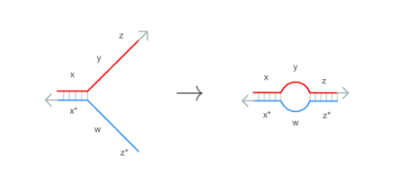
Figure S2: Bulge formation

Multiloop closing

— $k=($2.54\text{\times}{10}^{8}$)(\ell^{\prime}+5)^{-3}~{}${\mathrm{s}}^{-1}$$, where $\ell^{\prime}=\sum_{i=1}^{m}|d_{i}|+5(m-1)$ approximates the size of the multiloop containing domains $d_{1},d_{2},\ldots d_{m}$. We used a similar expression as for bulges, but must generalize to account for the presence of $m$ stems and loop segments within the multiloop. We therefore treat the multiloop size as the length of each domain, plus 5 nucleotides for each stem.

Opening

— $k=10^{6-1.24\ell}$. Note that 2,1 binding is the reverse reaction of 1,2 opening. Experimental evidence suggests this ratio depends exponentially on the length $\ell$ of the binding/opening domain ⁴⁹, and therefore:

$$e^{\Delta G^{\circ}/RT}=\frac{k_{\text{reverse}}}{k_{\text{forward}}}=\frac{\text{1,2 opening rate}}{\text{2,1 binding rate}}=10^{-a\ell}~{}$\mathrm{\text{M}}$$$

where $\Delta G^{\circ}$ is the Gibbs free energy at standard conditions, $T$ is the temperature in Kelvin, $R$ is the ideal gas constant, and $a$ is an unknown constant. Given the binding rate constant $k_{\text{forward}}=$1\text{\times}{10}^{6}\text{\,}{\mathrm{\text{M}}}^{-1}\text{\,}{\mathrm{s}}^{-1}$$, this means that the opening rate constant $k_{\text{reverse}}=10^{(6-a\ell)}~{}${\mathrm{s}}^{-1}$$. We know that the typical energy of a single base stack is $-1.7$ $\mathrm{\text{kcal}}\text{\,}{\mathrm{mol}}^{-1}$ at $T=298$ $\mathrm{K}$ (25 $\mathrm{\SIUnitSymbolCelsius}$) in a typical salt buffer⁴⁹. We can use this information to solve for the constant $a$:

$$e^{\Delta G^{\circ}/RT}=a10^{-\ell}\implies\Delta G^{\circ}=(-RT\ln 10)a\ell$$

$$\Delta G^{\circ}=-1.7\ell\implies-1.7\ell=(-RT\ln 10)a\ell$$

$$\implies a=1.7/(RT\ln 10)\approx 1.24$$

for $R$ = $1.99\text{\times}{10}^{-3}\text{\,}\mathrm{\text{kcal}}\text{\,}{\mathrm{K}}^{-1}\text{\,}{\mathrm{mol}}^{-1}$, $T$ = $298\text{\,}\mathrm{K}$.

3-way branch migration

— We can consider the 3-way branch migration process as consisting of an initiation step that takes some time $a~{}$\mathrm{s}$$ and a series of branch migration steps; the time for branch migration steps varies quadratically with the length $\ell$ of the domain ^{44, 50}, with some timescale $b~{}$\mathrm{s}$$ each. The expected time $\langle t\rangle$ for 3-way branch migration of $\ell$ bases, including an initiation time $b$, is

$$\langle t\rangle=a+b\ell^{2}.$$

Imperfectly approximating the completion time of branch migration as a Poisson rate with the same expected time, the rate constant $k$ is therefore

$$k=\frac{1}{\langle t\rangle}=\frac{1}{a+b\ell^{2}}$$

where the values of $a$ and $b$ must be determined experimentally, and represent the expected time for initiation and individual branch migration steps, respectively⁵⁰. We assume that the values are different for branch migration between adjacent domains ($d_{i,j}$ and $d_{i,j+1}$) and for remote toehold-mediated branch migration³⁵, where the domains are non-adjacent.

Adjacent

— $k=\left[($2.8\text{\times}{10}^{-3}$)+($0.1\text{\times}{10}^{-3}$)\ell^{2}\right]^{-1}~{}${\mathrm{s}}^{-1}$$. Srinivas et al. measured $a=$2.8\text{\times}{10}^{-3}\text{\,}\mathrm{s}$$ and $b=$0.1\text{\times}{10}^{-3}\text{\,}\mathrm{s}$$⁵⁰.

Remote toehold-mediated

— $k=\left[\rho(\ell)($2.8\text{\times}{10}^{-3}$)+($0.1\text{\times}{10}^{-3}$)\ell^{2}\right]^{-1}~{}${\mathrm{s}}^{-1}$$ We assume the same step rate $b$ as for adjacent branch migration above, but assume that the initiation time $a$ is a factor of $\rho(\ell^{\prime})$ slower for remote toehold-mediated branch migration than for adjacent branch migration. We define $\rho(\ell)=\alpha/k_{\text{multiloop closing}}(\ell^{\prime})$, where $k_{\text{multiloop closing}}(\ell^{\prime})$ is calculated by the rate constant formula given above for multiloop closing over a bulge length $\ell^{\prime}$, and $\alpha$ is a constant for remote toeholds, fitted to the experimental data.

4-way branch migration

— $k=\frac{1}{77+\ell^{2}}~{}${\mathrm{s}}^{-1}$$. We use a similar expression to that for 3-way branch migration. Dabby measured $a=$77\text{\,}\mathrm{s}$$ and $b=$1\text{\,}\mathrm{s}$$ ³⁶.

Appendix D Nucleic acid secondary structure and pseudoknots

Nucleic acid structures can be divided into two classes: those with base pairs that can be nested into a tree-like structure are called “non-pseudoknotted” (Fig. S3), while those that do not obey this nesting property are “pseudoknotted” ^{51, 52} (Fig. S4). There are vastly more possible pseudoknotted structures than non-pseudoknotted structures, so allowing enumeration of pseudoknotted intermediates greatly increases the possible size of the generated reaction network. It would be attractive to enumerate only a subset of pseudoknotted secondary structures, but a poor understanding of the energetics of pseudoknotted structures makes it very hard to determine which pseudoknots to allow and which to omit^{53, 54, 55}. Further, reactions (such as three-way branch migration) that are always plausible for non-pseudoknotted structures can yield topologically-impossible structures for pseudoknotted intermediates. For the sake of simplicity and efficiency we will therefore restrict our attention to non-pseudoknotted intermediates, for the time being.

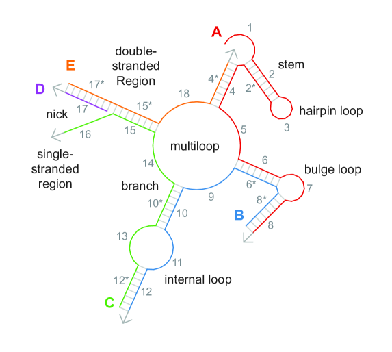
Figure S3: Non-pseudoknoted secondary structures. Our enumerator is capable of handling a wide range of non-pseudoknotted secondary structures, depicted above.

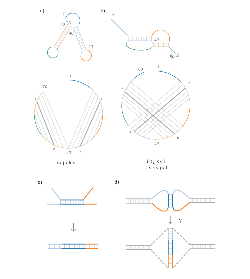
Figure S4: Pseudoknotted vs. non-pseudoknotted structures. (a) Structure containing no pseudoknots; all base pairs are either nested ($i<k<l<j$), or adjacent ($i<j<k<l$). (b) Structure containing a pseudoknot; $i<j$ and $k<l$, but $i<k<j<l$, so the nesting property is not satisfied. This can be seen geometrically in the circle diagram. (c) For non-pseudoknotted complexes, 1-1 binding is always permissible and yields plausible structures. (d) For a pseudoknotted complex such as this “kissing-loop” motif, binding between adjacent domains may produce unrealistic structures (e.g. binding between adjacent domains in the kissing-loop duplex would likely require partial unwinding of the duplexes). Lack of a coherent and efficient energetic model for structures with pseudoknots makes the plausibility of these structures difficult to evaluate.

Appendix E Limitations

As mentioned in the main text, there are two major limitations to the enumerator, as presented here.

The first limitation precludes several behaviors, such as partial binding between similar domains with small numbers of nucleotide mismatches (a concept which has been exploited to precisely control the thermodynamics and therefore specificity of DNA hybridization reactions ⁵⁶), as well as partial binding at the edges between two adjacent domains.

The second limitation precludes consideration of the wide range of structures that contain pseudoknots. The distinction between pseudoknotted and non-pseudoknotted complexes is demonstrated in Fig. S4 Essentially, a pseudoknotted complex is one which contains two intercalated stem-loop structures. Consider a complex with $N$ nucleotides, each numbered $1,2,\ldots,N$. Formally, this is non-pseudoknotted if, for every two base pairs $i,j$ and $k,l$ (where $i,j,k,l$ are the numerical indices of four nucleotides in a complex) where $i<j$, $k<l$, and $i<k$, then either $i<k<l<j$ (that is, the pair $k,l$ is nested within the pair $i,j$) or $i<j<k<l$ (that is, the pairs $i,j$ and $k,l$ occur sequentially). Pseudoknotted structures do not obey this nesting property. This can be easily seen by drawing the DNA backbone of a pseudoknotted structure around a circle, and drawing base pairs as chords of the circle; if these chords cross, a complex is pseudoknotted..

It should be apparent that there are combinatorially more pseudoknotted structures than non-pseudoknotted structures. The presence of pseudoknots has important implications for the energetics of a structure—notably, many parameters of the energetic models that incorporate pseudoknots have not been measured and as a consequence it is difficult to accurately calculate the free energy and therefore estimate the stability of pseudoknotted structures. Additionally, certain reactions have non-intuitive behavior; for instance, consider a 1-1 binding reaction between adjacent, complementary domains. For non-pseudoknotted structures, this reaction is always permissible. For pseudoknotted complexes, it is easy to consider scenarios where a naive branch migration would lead to physically implausible structures (see Fig. S4). For simplicity and efficiency, we therefore do not consider pseudoknotted complexes.

Appendix F Implementation

We have implemented the reaction enumeration algorithm, as well as the algorithm for condensing reactions, in a command-line utility written in Python. The enumerator allows input to be specified using the Pepper Intermediate Language (PIL)—a flexible, text-based language for describing DNA strand displacement systems ⁵⁷—as well as a simple, JSON-based interchange format. The enumerator can produce both full and condensed reaction spaces for a set of starting complexes. It can also write generated systems to several output formats:

Pepper Intermediate Language (PIL)

— Output format resembles input format ⁵⁷, but additional enumerated complexes and reactions are added.

Systems Biology Markup Language (SBML)⁵⁸

— Standard format used by many modeling packages in systems and synthetic biology. Allows models to be transferred to numerous simulation and analysis utilities.

Chemical Reaction Network (CRN)

— Simple plain text format listing each reaction on a single line. In this format, some reaction $A+B\to C+D$ would be written A + B -> C + D.

ENJS

— JSON-based output format; ENJS can be visualized interactively using DyNAMiC Workbench—this visualization is discussed in Chapter 2, and examples are shown in Chapter 6 of ref. ³⁰.

Appendix G Supplemental Pseudocode

Algorithm S1 Bind 1-1 move type

1:function bind11($c:\mathrm{Complex}$)

2:     $R\leftarrow\left\{~{}\right\}$ $\triangleright$ Initialize empty set of reactions

3:     $c=(S,T),S=\left\{s_{1},s_{2},\ldots s_{|S|}\right\}$

4:     for all $i\in\left\{1\ldots|S|\right\}$ do $\triangleright$ For each strand

5:         $s_{i}=(z,D)$

6:         for all $j\in\left\{1\ldots|D|\right\}$ do $\triangleright$ For each domain

7:              if $T_{i,j}=\varnothing$ then $\triangleright$ If domain $d_{j}$ is unpaired

8:                  $i^{\prime}\leftarrow i$

9:                  $j^{\prime}\leftarrow j+1$

10:                  while $i^{\prime}<|S|$ and $(i^{\prime},j^{\prime})\neq(i,j)$ do $\triangleright$ Iterate over all domains with higher indices

11:                       $s_{i^{\prime}}=(z^{\prime},D^{\prime}),D^{\prime}=\left\{d^{\prime}_{1},d^{\prime}_{2},\ldots\right\}$

12:                       if $j^{\prime}\geq|D^{\prime}|$ then $\triangleright$ If at the end of a strand

13:                           $(i^{\prime},j^{\prime})\leftarrow(i^{\prime}+1,0)$ $\triangleright$ Move to first domain on next strand

14:                       else if $T_{i^{\prime},j^{\prime}}\neq\varnothing$ then $\triangleright$ If domain is paired

15:                           $(i^{\prime},j^{\prime})\leftarrow T_{i^{\prime},j^{\prime}}$

16:$\triangleright$ Skip over the internal loop between $i,j$ and $i^{\prime},j^{\prime}$ so we don’t make a pseudoknot

17:                       else if $d_{j}={d^{\prime}}_{j^{\prime}}^{*}$ then $\triangleright$ If $d_{j}$ is complementary to $d_{j}^{\prime}$

18:                           $T^{\prime}\leftarrow T$ $\triangleright$ Make a new structure

19:                           $T^{\prime}_{i,j}\leftarrow(i^{\prime},j^{\prime})$, $T^{\prime}_{i^{\prime},j^{\prime}}\leftarrow(i,j)$ $\triangleright$ Where domains $(i,j)$ and $(i^{\prime},j^{\prime})$ are paired

20:                           $c^{\prime}\leftarrow(S,T^{\prime})$

21:                           $R\leftarrow R\cup\left\{(\BeginAccSupp{method=hex,unicode,ActualText=2983}\textnormal{\char 102\relax}\mathchoice{\mkern-4.05mu}{\mkern-4.05mu}{\mkern-4.3mu}{\mkern-4.8mu}\textnormal{\char 106\relax}\EndAccSupp{}c\BeginAccSupp{method=hex,unicode,ActualText=2984}\textnormal{\char 106\relax}\mathchoice{\mkern-4.05mu}{\mkern-4.05mu}{\mkern-4.3mu}{\mkern-4.8mu}\textnormal{\char 103\relax}\EndAccSupp{},\BeginAccSupp{method=hex,unicode,ActualText=2983}\textnormal{\char 102\relax}\mathchoice{\mkern-4.05mu}{\mkern-4.05mu}{\mkern-4.3mu}{\mkern-4.8mu}\textnormal{\char 106\relax}\EndAccSupp{}c^{\prime}\BeginAccSupp{method=hex,unicode,ActualText=2984}\textnormal{\char 106\relax}\mathchoice{\mkern-4.05mu}{\mkern-4.05mu}{\mkern-4.3mu}{\mkern-4.8mu}\textnormal{\char 103\relax}\EndAccSupp{})\right\}$ $\triangleright$ Make a new reaction that yields this complex

22:                       end if

23:                       $j^{\prime}\leftarrow j^{\prime}+1$ $\triangleright$ Go to next domain

24:                  end while

25:              end if

26:         end for

27:     end for

28:     return $R$

29:end function

Algorithm S2 Bind 2-1 move type

1:function bind21($c:\mathrm{Complex}$, $c^{\prime}:\mathrm{Complex}$)

2:     $R\leftarrow\left\{~{}\right\}$ $\triangleright$ Initialize empty set of reactions

3:     $c=(S,T)$, $c^{\prime}=(S^{\prime},T^{\prime})$

4:     for all $d$ such that $\exists(z,D)\in S$, $d\in D$ do $\triangleright$ For each domain on each strand in $c$

5:         for all $d^{\prime}$ such that $\exists(z^{\prime},D^{\prime})\in S^{\prime}$, $d^{\prime}\in D^{\prime}$ do $\triangleright$ For each domain on each strand in $c^{\prime}$

6:              if $d^{\prime}=d^{*}$ then $\triangleright$ If $d$ and $d^{\prime}$ are complementary

7:                  $S^{\prime\prime}\leftarrow S\cup S^{\prime}$

8:                  $T^{\prime\prime}\leftarrow$ combine structures, pair $d$ and $d^{\prime}$

9:                  $c^{\prime\prime}\leftarrow(S^{\prime\prime},T^{\prime\prime})$ $\triangleright$ Make new complex that joins $c$ and $c^{\prime}$

10:                  $R\leftarrow R\cup\left\{(\BeginAccSupp{method=hex,unicode,ActualText=2983}\textnormal{\char 102\relax}\mathchoice{\mkern-4.05mu}{\mkern-4.05mu}{\mkern-4.3mu}{\mkern-4.8mu}\textnormal{\char 106\relax}\EndAccSupp{}c,c^{\prime}\BeginAccSupp{method=hex,unicode,ActualText=2984}\textnormal{\char 106\relax}\mathchoice{\mkern-4.05mu}{\mkern-4.05mu}{\mkern-4.3mu}{\mkern-4.8mu}\textnormal{\char 103\relax}\EndAccSupp{},\BeginAccSupp{method=hex,unicode,ActualText=2983}\textnormal{\char 102\relax}\mathchoice{\mkern-4.05mu}{\mkern-4.05mu}{\mkern-4.3mu}{\mkern-4.8mu}\textnormal{\char 106\relax}\EndAccSupp{}c^{\prime\prime}\BeginAccSupp{method=hex,unicode,ActualText=2984}\textnormal{\char 106\relax}\mathchoice{\mkern-4.05mu}{\mkern-4.05mu}{\mkern-4.3mu}{\mkern-4.8mu}\textnormal{\char 103\relax}\EndAccSupp{})\right\}$ $\triangleright$ Make reaction that yields this complex

11:              end if

12:         end for

13:     end for

14:     return $R$

15:end function

Algorithm S3 Opening move type

1:function open($c:\mathrm{Complex}$)

2:     $R\leftarrow\left\{~{}\right\}$ $\triangleright$ Initialize empty set of reactions

3:     $c=(S,T),S=\left\{s_{1},s_{2},\ldots s_{|S|}\right\}$

4:     for all $i\in\left\{1\ldots|S|\right\}$ do $\triangleright$ For each strand

5:         $s_{i}=(z,D),D=\left\{d_{1},d_{2},\ldots d_{|D|}\right\}$

6:         for all $j\in\left\{1\ldots|D|\right\}$ do $\triangleright$ For each domain

7:              if $T_{i,j}\neq\varnothing$ and $T_{i,j}>(i,j)$ then $\triangleright$ If domain $d_{j}$ is paired to a later domain

8:$\triangleright$ Find the beginning and end of the helix where $d_{j}$ is bound

9:                  $A=(i_{A},j_{A})\leftarrow(i,j)$ $\triangleright$ Beginning of the helix on the “top” strand

10:                  $B=(i_{B},j_{B})\leftarrow T_{i,j}$ $\triangleright$ Beginning of the helix on the “bottom” strand

11:                  $A^{\prime}=(i_{A^{\prime}},j_{A^{\prime}})\leftarrow A$ $\triangleright$ End of the helix on the “top” strand

12:                  $B^{\prime}=(i_{B^{\prime}},j_{B^{\prime}})\leftarrow B$ $\triangleright$ End of the helix on the “bottom” strand

13:                  $\ell\leftarrow|d_{j}|$ $\triangleright$ Keep track of helix length in nucleotides

14:                  $\triangleright$ Find the end of the helix

15:                  while $j_{A}^{\prime}<|s_{i_{A^{\prime}}}|$ and $j_{B}^{\prime}\geq 0$ and $A^{\prime}=T_{B^{\prime}}$ do $\triangleright$ While neither strand is broken and domains are paired

16:                       $j_{A^{\prime}}\leftarrow j_{A^{\prime}}+1$ $\triangleright$ Move right

17:                       $j_{B^{\prime}}\leftarrow j_{B^{\prime}}-1$

18:                       $\ell\leftarrow\ell+|d_{j_{A^{\prime}}}|$

19:                  end while

20:                  $\triangleright$ Find the beginning of the helix

21:                  while $j_{A}\geq 0$ and $j_{B}<|s_{i_{B}}|$ and $A=T_{B}$ do $\triangleright$ While neither strand is broken and domains are paired

22:                       $j_{A}\leftarrow j_{A}-1$ $\triangleright$ Move left

23:                       $j_{B}\leftarrow j_{B}+1$

24:                       $\ell\leftarrow\ell+|d_{j_{A}}|$

25:                  end while

26:                  if $\ell<L$ then $\triangleright$ If the total length of the helix is less than the threshold

27:                       $T^{\prime}\leftarrow T$

28:                       for all $j^{\prime}\in\left\{j_{A}\ldots j_{A^{\prime}}\right\}$ do

29:                           Update $T^{\prime}$ to break pair $i,j^{\prime}$

30:                       end for

31:                       if $S,T^{\prime}$ is not connected then

32:                           $c^{\prime},c^{\prime\prime}\leftarrow$ split $T^{\prime}$ and $S$ into two connected complexes

33:                           $R\leftarrow R\cup\left\{(\BeginAccSupp{method=hex,unicode,ActualText=2983}\textnormal{\char 102\relax}\mathchoice{\mkern-4.05mu}{\mkern-4.05mu}{\mkern-4.3mu}{\mkern-4.8mu}\textnormal{\char 106\relax}\EndAccSupp{}c\BeginAccSupp{method=hex,unicode,ActualText=2984}\textnormal{\char 106\relax}\mathchoice{\mkern-4.05mu}{\mkern-4.05mu}{\mkern-4.3mu}{\mkern-4.8mu}\textnormal{\char 103\relax}\EndAccSupp{},\BeginAccSupp{method=hex,unicode,ActualText=2983}\textnormal{\char 102\relax}\mathchoice{\mkern-4.05mu}{\mkern-4.05mu}{\mkern-4.3mu}{\mkern-4.8mu}\textnormal{\char 106\relax}\EndAccSupp{}c^{\prime},c^{\prime\prime}\BeginAccSupp{method=hex,unicode,ActualText=2984}\textnormal{\char 106\relax}\mathchoice{\mkern-4.05mu}{\mkern-4.05mu}{\mkern-4.3mu}{\mkern-4.8mu}\textnormal{\char 103\relax}\EndAccSupp{})\right\}$ $\triangleright$ Make reaction that yields these complexes

34:                       else

35:                           $c^{\prime}\leftarrow(S,T^{\prime})$ $\triangleright$ Make new complex

36:                           $R\leftarrow R\cup\left\{(\BeginAccSupp{method=hex,unicode,ActualText=2983}\textnormal{\char 102\relax}\mathchoice{\mkern-4.05mu}{\mkern-4.05mu}{\mkern-4.3mu}{\mkern-4.8mu}\textnormal{\char 106\relax}\EndAccSupp{}c\BeginAccSupp{method=hex,unicode,ActualText=2984}\textnormal{\char 106\relax}\mathchoice{\mkern-4.05mu}{\mkern-4.05mu}{\mkern-4.3mu}{\mkern-4.8mu}\textnormal{\char 103\relax}\EndAccSupp{},\BeginAccSupp{method=hex,unicode,ActualText=2983}\textnormal{\char 102\relax}\mathchoice{\mkern-4.05mu}{\mkern-4.05mu}{\mkern-4.3mu}{\mkern-4.8mu}\textnormal{\char 106\relax}\EndAccSupp{}c^{\prime}\BeginAccSupp{method=hex,unicode,ActualText=2984}\textnormal{\char 106\relax}\mathchoice{\mkern-4.05mu}{\mkern-4.05mu}{\mkern-4.3mu}{\mkern-4.8mu}\textnormal{\char 103\relax}\EndAccSupp{})\right\}$ $\triangleright$ Make reaction that yields this complex

37:                       end if

38:                  end if

39:              end if

40:         end for

41:     end for

42:     return $R$

43:end function

Algorithm S4 3-way branch migration move type

1:function 3way($c:\mathrm{Complex}$)

2:     $R\leftarrow\left\{~{}\right\}$ $\triangleright$ Initialize empty set of reactions

3:     $c=(S,T),S=\left\{s_{1},s_{2},\ldots s_{|S|}\right\}$

4:     for all $i\in\left\{1\ldots|S|\right\}$ do $\triangleright$ For each strand

5:         $s_{i}=(z,D),D=\left\{d_{1},d_{2},\ldots d_{|D|}\right\}$

6:         for all $j\in\left\{1\ldots|D|\right\}$ do $\triangleright$ For each domain

7:              $\triangleright$ Look to the left

8:              if $T_{i,j}\neq\varnothing$ and $j\neq|D|$ and $T_{i,j+1}=\varnothing$ then

9:                  $(i^{\prime},j^{\prime})\leftarrow(i,j+1)$ $\triangleright$ $(i,j+1)$ will be the invading domain

10:                  repeat$\triangleright$ Search left to find a bound domain $(i^{\prime},j^{\prime})$ that can be displaced

11:                       $j^{\prime}\leftarrow j^{\prime}-1$

12:                       if $T_{i^{\prime},j^{\prime}}\neq\varnothing$ and $d_{i^{\prime},j^{\prime}}$ can pair $d_{j+1}$ then

13:                           $T^{\prime}\leftarrow T$ where $T^{\prime}_{i^{\prime},j^{\prime}}=(i,j+1)$, $T^{\prime}_{i,j+1}=(i^{\prime},j^{\prime})$

14:                           if $S,T^{\prime}$ is not connected then

15:                                $c^{\prime},c^{\prime\prime}\leftarrow$ split $T^{\prime}$ and $S$ into two connected complexes

16:                                $R\leftarrow R\cup\left\{(\BeginAccSupp{method=hex,unicode,ActualText=2983}\textnormal{\char 102\relax}\mathchoice{\mkern-4.05mu}{\mkern-4.05mu}{\mkern-4.3mu}{\mkern-4.8mu}\textnormal{\char 106\relax}\EndAccSupp{}c\BeginAccSupp{method=hex,unicode,ActualText=2984}\textnormal{\char 106\relax}\mathchoice{\mkern-4.05mu}{\mkern-4.05mu}{\mkern-4.3mu}{\mkern-4.8mu}\textnormal{\char 103\relax}\EndAccSupp{},\BeginAccSupp{method=hex,unicode,ActualText=2983}\textnormal{\char 102\relax}\mathchoice{\mkern-4.05mu}{\mkern-4.05mu}{\mkern-4.3mu}{\mkern-4.8mu}\textnormal{\char 106\relax}\EndAccSupp{}c^{\prime},c^{\prime\prime}\BeginAccSupp{method=hex,unicode,ActualText=2984}\textnormal{\char 106\relax}\mathchoice{\mkern-4.05mu}{\mkern-4.05mu}{\mkern-4.3mu}{\mkern-4.8mu}\textnormal{\char 103\relax}\EndAccSupp{})\right\}$ $\triangleright$ Make reaction that yields these complexes

17:                           else

18:                                $c^{\prime}\leftarrow(S,T^{\prime})$ $\triangleright$ Make new complex

19:                                $R\leftarrow R\cup\left\{(\BeginAccSupp{method=hex,unicode,ActualText=2983}\textnormal{\char 102\relax}\mathchoice{\mkern-4.05mu}{\mkern-4.05mu}{\mkern-4.3mu}{\mkern-4.8mu}\textnormal{\char 106\relax}\EndAccSupp{}c\BeginAccSupp{method=hex,unicode,ActualText=2984}\textnormal{\char 106\relax}\mathchoice{\mkern-4.05mu}{\mkern-4.05mu}{\mkern-4.3mu}{\mkern-4.8mu}\textnormal{\char 103\relax}\EndAccSupp{},\BeginAccSupp{method=hex,unicode,ActualText=2983}\textnormal{\char 102\relax}\mathchoice{\mkern-4.05mu}{\mkern-4.05mu}{\mkern-4.3mu}{\mkern-4.8mu}\textnormal{\char 106\relax}\EndAccSupp{}c^{\prime}\BeginAccSupp{method=hex,unicode,ActualText=2984}\textnormal{\char 106\relax}\mathchoice{\mkern-4.05mu}{\mkern-4.05mu}{\mkern-4.3mu}{\mkern-4.8mu}\textnormal{\char 103\relax}\EndAccSupp{})\right\}$ $\triangleright$ Make reaction that yields this complex

20:                           end if

21:                       end if

22:                       $(i^{\prime},j^{\prime})\leftarrow T_{i^{\prime},j^{\prime}}$ $\triangleright$ Follow the structure

23:                  until $j^{\prime}=-1$ or $T_{i^{\prime},j^{\prime}}=\varnothing$ or $(i^{\prime},j^{\prime})=(i,j)$

24:              end if

25:              $\triangleright$ Look to the right

26:              if $T_{i,j}\neq\varnothing$ and $j\neq 0$ and $T_{i,j-1}=\varnothing$ then

27:                  $(i^{\prime},j^{\prime})\leftarrow(i,j-1)$ $\triangleright$ $(i,j-1)$ will be the invading domain

28:                  repeat$\triangleright$ Search right to find a bound domain $(i^{\prime},j^{\prime})$ that can be displaced

29:                       $j^{\prime}\leftarrow j^{\prime}+1$

30:                       if $T_{i^{\prime},j^{\prime}}\neq\varnothing$ and $d_{i^{\prime},j^{\prime}}$ can pair $d_{j-1}$ then

31:                           $T^{\prime}\leftarrow T$ where $T^{\prime}_{i^{\prime},j^{\prime}}=(i,j-1)$, $T^{\prime}_{i,j-1}=(i^{\prime},j^{\prime})$

32:                           if $S,T^{\prime}$ is not connected then

33:                                $c^{\prime},c^{\prime\prime}\leftarrow$ split $T^{\prime}$ and $S$ into two connected complexes

34:                                $R\leftarrow R\cup\left\{(\BeginAccSupp{method=hex,unicode,ActualText=2983}\textnormal{\char 102\relax}\mathchoice{\mkern-4.05mu}{\mkern-4.05mu}{\mkern-4.3mu}{\mkern-4.8mu}\textnormal{\char 106\relax}\EndAccSupp{}c\BeginAccSupp{method=hex,unicode,ActualText=2984}\textnormal{\char 106\relax}\mathchoice{\mkern-4.05mu}{\mkern-4.05mu}{\mkern-4.3mu}{\mkern-4.8mu}\textnormal{\char 103\relax}\EndAccSupp{},\BeginAccSupp{method=hex,unicode,ActualText=2983}\textnormal{\char 102\relax}\mathchoice{\mkern-4.05mu}{\mkern-4.05mu}{\mkern-4.3mu}{\mkern-4.8mu}\textnormal{\char 106\relax}\EndAccSupp{}c^{\prime},c^{\prime\prime}\BeginAccSupp{method=hex,unicode,ActualText=2984}\textnormal{\char 106\relax}\mathchoice{\mkern-4.05mu}{\mkern-4.05mu}{\mkern-4.3mu}{\mkern-4.8mu}\textnormal{\char 103\relax}\EndAccSupp{})\right\}$ $\triangleright$ Make reaction that yields these complexes

35:                           else

36:                                $c^{\prime}\leftarrow(S,T^{\prime})$ $\triangleright$ Make new complex

37:                                $R\leftarrow R\cup\left\{(\BeginAccSupp{method=hex,unicode,ActualText=2983}\textnormal{\char 102\relax}\mathchoice{\mkern-4.05mu}{\mkern-4.05mu}{\mkern-4.3mu}{\mkern-4.8mu}\textnormal{\char 106\relax}\EndAccSupp{}c\BeginAccSupp{method=hex,unicode,ActualText=2984}\textnormal{\char 106\relax}\mathchoice{\mkern-4.05mu}{\mkern-4.05mu}{\mkern-4.3mu}{\mkern-4.8mu}\textnormal{\char 103\relax}\EndAccSupp{},\BeginAccSupp{method=hex,unicode,ActualText=2983}\textnormal{\char 102\relax}\mathchoice{\mkern-4.05mu}{\mkern-4.05mu}{\mkern-4.3mu}{\mkern-4.8mu}\textnormal{\char 106\relax}\EndAccSupp{}c^{\prime}\BeginAccSupp{method=hex,unicode,ActualText=2984}\textnormal{\char 106\relax}\mathchoice{\mkern-4.05mu}{\mkern-4.05mu}{\mkern-4.3mu}{\mkern-4.8mu}\textnormal{\char 103\relax}\EndAccSupp{})\right\}$ $\triangleright$ Make reaction that yields this complex

38:                           end if

39:                       end if

40:                  until $j^{\prime}=|D|$ or $(i^{\prime},j^{\prime})=(i,j)$

41:              end if

42:         end for

43:     end for

44:     return $R$

45:end function

Algorithm S5 4-way branch migration move type

1:function 4way($c:\mathrm{Complex}$)

2:     $R\leftarrow\left\{~{}\right\}$ $\triangleright$ Initialize empty set of reactions

3:     $c=(S,T),S=\left\{s_{1},s_{2},\ldots s_{|S|}\right\}$

4:     for all $i\in\left\{1\ldots|S|\right\}$ do $\triangleright$ For each strand

5:         $s_{i}=(z,D),D=\left\{d_{1},d_{2},\ldots d_{|D|}\right\}$

6:         for all $j\in\left\{1\ldots|D|\right\}$ do $\triangleright$ For each domain

7:              if $T_{i,j}\neq\varnothing$ and $j<|D|$ then $\triangleright$ domain $d_{j}$ must be bound, not be at the end of a strand

8:                  $A\leftarrow(i,j+1)$ $\triangleright$ Displacing domain

9:                  $B\leftarrow T_{i,j+1}$ $\triangleright$ Displaced domain

10:                  if $B=\varnothing$ then Continue

11:                  end if

12:                  $C=(i_{C},j_{C})\leftarrow T_{i,j}$

13:                  $C\leftarrow(i_{C},j_{C}-1)$ $\triangleright$ Template domain (replaces B, binds A)

14:                  if $j_{C}<1$ then Continue

15:                  end if

16:                  $D\leftarrow T_{C}$ $\triangleright$ (replaces A, binds B)

17:                  if $D=\varnothing$ then Continue

18:                  end if

19:                  if $B\neq C$ and $d_{A}=d_{C}^{*}$ and $d_{B}=d_{D}^{*}$ then $\triangleright$ If this is a four-way branch migration

20:                       $T^{\prime}\leftarrow T$, $T^{\prime}_{A}\leftarrow C,T^{\prime}_{C}\leftarrow A$; $T^{\prime}_{B}\leftarrow D,T^{\prime}_{D}\leftarrow B$

21:                       if $S,T^{\prime}$ is not connected then

22:                           $c^{\prime},c^{\prime\prime}\leftarrow$ split $T^{\prime}$ and $S$ into two connected complexes

23:                           $R\leftarrow R\cup\left\{(\BeginAccSupp{method=hex,unicode,ActualText=2983}\textnormal{\char 102\relax}\mathchoice{\mkern-4.05mu}{\mkern-4.05mu}{\mkern-4.3mu}{\mkern-4.8mu}\textnormal{\char 106\relax}\EndAccSupp{}c\BeginAccSupp{method=hex,unicode,ActualText=2984}\textnormal{\char 106\relax}\mathchoice{\mkern-4.05mu}{\mkern-4.05mu}{\mkern-4.3mu}{\mkern-4.8mu}\textnormal{\char 103\relax}\EndAccSupp{},\BeginAccSupp{method=hex,unicode,ActualText=2983}\textnormal{\char 102\relax}\mathchoice{\mkern-4.05mu}{\mkern-4.05mu}{\mkern-4.3mu}{\mkern-4.8mu}\textnormal{\char 106\relax}\EndAccSupp{}c^{\prime},c^{\prime\prime}\BeginAccSupp{method=hex,unicode,ActualText=2984}\textnormal{\char 106\relax}\mathchoice{\mkern-4.05mu}{\mkern-4.05mu}{\mkern-4.3mu}{\mkern-4.8mu}\textnormal{\char 103\relax}\EndAccSupp{})\right\}$ $\triangleright$ Make reaction that yields these complexes

24:                       else

25:                           $c^{\prime}\leftarrow(S,T^{\prime})$ $\triangleright$ Make new complex

26:                           $R\leftarrow R\cup\left\{(\BeginAccSupp{method=hex,unicode,ActualText=2983}\textnormal{\char 102\relax}\mathchoice{\mkern-4.05mu}{\mkern-4.05mu}{\mkern-4.3mu}{\mkern-4.8mu}\textnormal{\char 106\relax}\EndAccSupp{}c\BeginAccSupp{method=hex,unicode,ActualText=2984}\textnormal{\char 106\relax}\mathchoice{\mkern-4.05mu}{\mkern-4.05mu}{\mkern-4.3mu}{\mkern-4.8mu}\textnormal{\char 103\relax}\EndAccSupp{},\BeginAccSupp{method=hex,unicode,ActualText=2983}\textnormal{\char 102\relax}\mathchoice{\mkern-4.05mu}{\mkern-4.05mu}{\mkern-4.3mu}{\mkern-4.8mu}\textnormal{\char 106\relax}\EndAccSupp{}c^{\prime}\BeginAccSupp{method=hex,unicode,ActualText=2984}\textnormal{\char 106\relax}\mathchoice{\mkern-4.05mu}{\mkern-4.05mu}{\mkern-4.3mu}{\mkern-4.8mu}\textnormal{\char 103\relax}\EndAccSupp{})\right\}$ $\triangleright$ Make reaction that yields this complex

27:                       end if

28:                  end if

29:              end if

30:         end for

31:     end for

32:     return $R$

33:end function

Algorithm S6 Reaction enumeration

1:procedure Enumerate($A:\left\{\mathrm{Complex}\right\}$)

2:     $\mathcal{E}\leftarrow\left\{\right\};\mathcal{S}\leftarrow\left\{\right\};\mathcal{T}\leftarrow\left\{\right\}$ $\triangleright$ Complexes

3:     $\mathcal{R}\leftarrow\left\{\right\}$ $\triangleright$ Reactions

4:     $\mathcal{Q}\leftarrow\left\{\right\}$ $\triangleright$ Resting states

5:     $\mathcal{B}\leftarrow A$

6:     while  $\mathcal{B}\neq\left\{\right\}$  do $\triangleright$ Enumerate fast reactions from $A$

7:         $b\leftarrow$ pop($\mathcal{B}$)

8:         $(S^{\prime},T^{\prime},Q^{\prime},R^{\prime})\leftarrow$ enumerateNeighborhood($b$) $\triangleright$ Find fast reactions from $b$

9:         $\mathcal{S}\leftarrow\mathcal{S}\cup S^{\prime}$; $\mathcal{T}\leftarrow\mathcal{T}\cup T^{\prime}$; $\mathcal{R}\leftarrow\mathcal{R}\cup R^{\prime}$; $\mathcal{Q}\leftarrow\mathcal{Q}\cup Q^{\prime}$

10:     end while

11:     while $\mathcal{S}\neq\left\{\right\}$ do $\triangleright$ Enumerate slow reactions between resting state complexes

12:         $s\leftarrow$ pop($\mathcal{S}$)

13:         $(R^{\prime},B^{\prime})\leftarrow$ getSlowReactions($s$, $\mathcal{S}\cup\mathcal{E}$) $\triangleright$ Find slow reactions from $s$

14:         $\mathcal{E}\leftarrow\mathcal{E}\cup\left\{s\right\}$ $\triangleright$ $s$ moves to $\mathcal{E}$ once slow reactions are enumerated

15:         $\mathcal{R}\leftarrow\mathcal{R}\cup R^{\prime}$ $\triangleright$ Store new reactions

16:         $\mathcal{B}\leftarrow\mathcal{B}\cup B^{\prime}\setminus(\mathcal{E}\cup\mathcal{S}\cup{T})$ $\triangleright$ Store new complexes

17:         while  $\mathcal{B}\neq\left\{\right\}$  do $\triangleright$ Enumerate fast reactions from $B$

18:              $b\leftarrow$ pop($\mathcal{B}$)

19:              $(S^{\prime},T^{\prime},Q^{\prime},R^{\prime})\leftarrow$ neighborhood($b$) $\triangleright$ Find fast reactions from $b$

20:              $\mathcal{S}\leftarrow\mathcal{S}\cup S^{\prime}$; $\mathcal{T}\leftarrow\mathcal{T}\cup T^{\prime}$; $\mathcal{R}\leftarrow\mathcal{R}\cup R^{\prime}$; $\mathcal{Q}\leftarrow\mathcal{Q}\cup Q^{\prime}$

21:         end while

22:     end while

23:end procedure

24:procedure enumerateNeighborhood($c:\mathrm{Complex}$) $\triangleright$ Calculates fast reactions from $c$, sorts complexes into resting state complexes/transient complexes

25:     $\mathcal{F}=\{c\}$ $\triangleright$ Complexes from fast reactions in neighborhood

26:     $\mathcal{N}=\left\{\right\}$ $\triangleright$ Complexes in neighborhood

27:     $\mathcal{R}_{N}=\left\{\right\}$ $\triangleright$ (Fast) Reactions in neighborhood

28:     while  $\mathcal{F}\neq\left\{\right\}$  do $\triangleright$ Enumerate fast reactions from each complex in $F$

29:         $f\leftarrow$ pop($\mathcal{F}$)

30:         $(R^{\prime},F^{\prime})\leftarrow$ getFastReactions($f$) $\triangleright$ Find fast reactions from $f$

31:         $\mathcal{F}\leftarrow\mathcal{F}\cup F^{\prime}\setminus\mathcal{N}$

32:         $\mathcal{N}\leftarrow\mathcal{N}\cup F^{\prime}$

33:         $\mathcal{R}_{N}\leftarrow\mathcal{R}_{N}\cup R^{\prime}$

34:     end while

35:     Apply Tarjan’s algorithm⁵⁹ to find strongly-connected components of the directed graph $G=(\mathcal{N},\mathcal{R}_{N})$

36:     $Q^{\prime}\leftarrow\left\{\text{strongly-connected components of }G\text{ with no outgoing fast reactions}\right\}$ $\triangleright$ Resting states are SCCs of $G$

37:     $S^{\prime}\leftarrow\left\{s:s\in q~{}\text{for any}~{}q\in Q^{\prime}\right\}$ $\triangleright$ resting state complexes are in a resting state

38:     $T^{\prime}\leftarrow\mathcal{N}\setminus S^{\prime}$ $\triangleright$ Transient complexes are everything else

39:     return $(S^{\prime},T^{\prime},Q^{\prime},\mathcal{R}_{N})$

40:end procedure

41:procedure getFastReactions($c:\mathrm{Complex}$)

42:$\triangleright$ Calculates all fast (unimolecular) reactions that consume $c$

43:     $R\leftarrow$ fast reactions consuming $c$, $C\leftarrow$ union of products of reactions in $R$

44:     return $R,C$

45:end procedure

46:procedure getSlowReactions($c:\mathrm{Complex}$, $S:\left\{\mathrm{Complex}\right\}$)

47:$\triangleright$ Calculates all slow (bimolecular) reactions that consume $c$ and an element of $S$

48:     $R\leftarrow$ slow reactions consuming $c$ and $s\in S$, $C\leftarrow$ union of products of reactions in $R$

49:     return $R,C$

50:end procedure

Algorithm S7 Condensing Reactions

1:$\mathbb{F}{x}\leftarrow$ undefined $\forall$ complexes $x$ $\triangleright$ The map $\mathbb{F}:\mathrm{Complex}\to\left\{\mathrm{Fate}\right\}$ is global and begins empty

2:$S\leftarrow\left\{~{}\right\}$ $\triangleright$ The map $S:\mathrm{Complex}\to\left\{\mathrm{Complex}\right\}$ is global and begins empty

3:

4:procedure Condense($\mathcal{C}:\left\{\mathrm{Complex}\right\}$, $\mathcal{R}:\left\{\mathrm{Reaction}\right\}$) $\triangleright$ Computes the fates for each complex, then generates a set of condensed reactions

5:     $\mathcal{R}_{s}\leftarrow\left\{r:r\in\mathcal{R},r~{}\text{is slow}\right\}$ $\triangleright$ Slow reactions

6:     $\mathcal{R}_{f}\leftarrow\mathcal{R}\setminus\mathcal{R}_{s}$ $\triangleright$ Fast reactions

7:     $\mathcal{R}_{f}^{(1,1)}\leftarrow\left\{r\in\mathcal{R}_{f}:\alpha(r)=(1,1)\right\}$ $\triangleright$ Fast (1,1) reactions

8:     Use Tarjan’s algorithm⁵⁹ to compute the set of strongly-connected components

9:from the graph $\Gamma=(\mathcal{C},\mathcal{R}_{f}^{(1,1)})$

10:     $S\leftarrow$ the set of strongly-connected components of $\Gamma$

11:     $\mathbb{S}(x)\leftarrow$ the strongly-connected component containing complex $x$, $\forall x\in\mathcal{C}$

12:     for all $\mathcal{C}_{c}\in S$ do $\triangleright$ For each SCC $\mathcal{C}_{c}$ of $\Gamma$

13:         computeFates($C_{c}$, $\mathcal{R}_{f}$)

14:     end for

15:     return condenseReactions($\mathcal{R}_{s}$)

16:end procedure

17:

18:procedure computeFates($\mathcal{C}:\left\{\mathrm{Complex}\right\}$, $\mathcal{R}_{f}:\left\{\mathrm{Reaction}\right\}$)

19:     $R_{o}\leftarrow\left\{r=(A,B)\in\mathcal{R}_{f}:A\subseteq\mathcal{C},B\setminus\mathcal{C}\neq\emptyset\right\}$ $\triangleright$ Outgoing fast reactions

20:     if $|R_{o}|=0$ then $\triangleright$ If no outgoing fast reactions

21:         $\mathbb{F}(c)\leftarrow\BeginAccSupp{method=hex,unicode,ActualText=2983}\textnormal{\char 102\relax}\mathchoice{\mkern-4.05mu}{\mkern-4.05mu}{\mkern-4.3mu}{\mkern-4.8mu}\textnormal{\char 106\relax}\EndAccSupp{}\mathcal{C}\BeginAccSupp{method=hex,unicode,ActualText=2984}\textnormal{\char 106\relax}\mathchoice{\mkern-4.05mu}{\mkern-4.05mu}{\mkern-4.3mu}{\mkern-4.8mu}\textnormal{\char 103\relax}\EndAccSupp{}~{}\forall~{}c\in\mathcal{C}$ $\triangleright$ $\mathbb{F}(c)$ is the resting state $\mathcal{C}$ containing the complex $c$

22:     else$\triangleright$ If there are outgoing fast reactions

23:         for all $c\in\mathcal{C}$ do

24:              $R_{o}^{(}1,n)\leftarrow\left\{r\in R_{o}:\alpha(r)=(1,n)\right\}$

25:              $P_{o}\leftarrow\bigcup_{r=(A,B)\in R_{o}^{(}1,1)}B$

26:              for all $x\in P_{o}$ do

27:                  If $\mathbb{F}(x)$ is undefined, computeFates($\mathbb{S}(x)$, $\mathcal{R}_{f}$)

28:              end for

29:              $\mathbb{F}(c)\leftarrow\displaystyle\bigcup_{r=(A,B)\in R_{o}}\left(\bigoplus_{b\in B}\mathbb{F}(b)\right)$ $\triangleright$ $\mathbb{F}(c)$ are the possible fates from outgoing reactions

30:         end for

31:     end if

32:end procedure

33:

34:procedure condenseReactions($\mathcal{R}_{s}:\left\{\mathrm{Reaction}\right\}$) $\triangleright$ Condensed reaction space from the set of slow reactions

35:     $\mathcal{\hat{R}}\leftarrow\left\{~{}\right\}$ $\triangleright$ Condensed reactions

36:     for all $s=(A,{b})\in\mathcal{R}_{s}$ do

37:         $A^{\prime}\leftarrow\sum_{a\in A}\mathbb{F}(a)$ $\triangleright$ Fates of reactants are all trivial

38:         for all $B^{\prime}\in\mathbb{F}(b)$ do $\triangleright$ For each fate of $b$

39:              $r^{\prime}\leftarrow(A^{\prime},B^{\prime})$ $\triangleright$ Generate new reaction

40:              $\mathcal{\hat{R}}\leftarrow\mathcal{\hat{R}}\cup{r^{\prime}}$

41:         end for

42:     end for

43:     return $\mathcal{\hat{R}}$

44:end procedure

References

- [1] D. Y. Zhang and G. Seelig, “Dynamic DNA nanotechnology using strand-displacement reactions.,” Nat. Chem., vol. 3, pp. 103–113, 2011.
- [2] Y. Krishnan and F. C. Simmel, “Nucleic Acid Based Molecular Devices,” Angew. Chem. Int. Ed., vol. 50, pp. 3124–3156, Mar. 2011.
- [3] N. C. Seeman, “Nanomaterials based on DNA.,” Annu. Rev. Biochem., vol. 79, pp. 65–87, 2010.
- [4] X. Chen and A. Ellington, “Shaping up nucleic acid computation,” Curr. Opin. Biotechnol., 2010.
- [5] E. Winfree, F. Liu, L. A. Wenzler, and N. C. Seeman, “Design and self-assembly of two-dimensional DNA crystals.,” Nature, vol. 394, pp. 539–544, Aug. 1998.
- [6] P. W. K. Rothemund, N. Papadakis, and E. Winfree, “Algorithmic self-assembly of DNA Sierpinski triangles.,” PLoS Biol., vol. 2, p. e424, 2004.
- [7] P. W. K. Rothemund, “Folding DNA to create nanoscale shapes and patterns,” Nature, vol. 440, pp. 297–302, Mar. 2006.
- [8] B. Wei, M. Dai, and P. Yin, “Complex shapes self-assembled from single-stranded DNA tiles.,” Nature, vol. 485, pp. 623–626, May 2012.
- [9] B. Yurke, A. J. Turberfield, A. P. Mills, F. C. Simmel, and J. L. Neumann, “A DNA-fuelled molecular machine made of DNA.,” Nature, vol. 406, pp. 605–608, Aug. 2000.
- [10] A. J. Turberfield, J. C. Mitchell, B. Yurke, A. P. Mills, M. I. Blakey, and F. C. Simmel, “DNA fuel for free-running nanomachines.,” Phys. Rev. Lett., vol. 90, p. 118102, Mar. 2003.
- [11] S. Venkataraman, R. M. Dirks, P. W. K. Rothemund, E. Winfree, and N. A. Pierce, “An autonomous polymerization motor powered by DNA hybridization,” Nat. Nanotech., vol. 2, pp. 490–494, July 2007.
- [12] J.-S. Shin and N. A. Pierce, “A synthetic DNA walker for molecular transport.,” J. Am. Chem. Soc., vol. 126, pp. 10834–10835, Sept. 2004.
- [13] W. B. Sherman and N. C. Seeman, “A precisely controlled DNA biped walking device,” Nano Lett., 2004.
- [14] P. Yin, H. M. T. Choi, C. R. Calvert, and N. A. Pierce, “Programming biomolecular self-assembly pathways.,” Nature, vol. 451, pp. 318–322, 2008.
- [15] T. Omabegho, R. Sha, and N. C. Seeman, “A bipedal DNA Brownian motor with coordinated legs.,” Science, vol. 324, pp. 67–71, Apr. 2009.
- [16] B. Ding and N. C. Seeman, “Operation of a DNA Robot Arm Inserted into a 2D DNA Crystalline Substrate,” Science, vol. 314, pp. 1583–1585, Dec. 2006.
- [17] R. A. Muscat, J. Bath, and A. J. Turberfield, “A Programmable Molecular Robot,” Nano Lett., vol. 11, pp. 982–987, Mar. 2011.
- [18] D. Y. Zhang, A. J. Turberfield, B. Yurke, and E. Winfree, “Engineering entropy-driven reactions and networks catalyzed by DNA,” Science, vol. 318, pp. 1121–1125, Nov. 2007.
- [19] B. Li, Y. Jiang, X. Chen, and A. D. Ellington, “Probing spatial organization of DNA strands using enzyme-free hairpin assembly circuits,” J. Am. Chem. Soc., vol. 134, pp. 13918–13921, Aug. 2012.
- [20] R. M. Dirks and N. A. Pierce, “Triggered amplification by hybridization chain reaction.,” Proc. Natl. Acad. Sci. U. S. A., vol. 101, pp. 15275–15278, Oct. 2004.
- [21] J. Kim and E. Winfree, “Synthetic in vitro transcriptional oscillators,” Molecular systems biology, vol. 7, no. 1, 2011.
- [22] G. Seelig, D. Soloveichik, D. Y. Zhang, and E. Winfree, “Enzyme-Free Nucleic Acid Logic Circuits,” Science, vol. 314, pp. 1585–1588, 2006.
- [23] L. Qian, D. Soloveichik, and E. Winfree, “Efficient Turing-universal computation with DNA polymers,” DNA Computing and Molecular Programming, pp. 123–140, 2011.
- [24] L. Qian, E. Winfree, and J. Bruck, “Neural network computation with DNA strand displacement cascades.,” Nature, vol. 475, pp. 368–372, 2011.
- [25] L. Qian and E. Winfree, “Scaling up digital circuit computation with DNA strand displacement cascades.,” Science, vol. 332, pp. 1196–1201, 2011.
- [26] Y.-J. Chen, N. Dalchau, N. Srinivas, A. Phillips, L. Cardelli, D. Soloveichik, and G. Seelig, “Programmable chemical controllers made from DNA,” Nat. Nanotech., vol. 8, pp. 755–762, 2013.
- [27] J. N. Zadeh, C. D. Steenberg, J. S. Bois, B. R. Wolfe, M. B. Pierce, A. R. Khan, R. M. Dirks, and N. A. Pierce, “NUPACK: Analysis and design of nucleic acid systems.,” J. Comput. Chem., vol. 32, pp. 170–173, Jan. 2011.
- [28] D. Y. Zhang, “Towards domain-based sequence design for DNA strand displacement reactions,” Lecture Notes in Computer Science, vol. 6518, pp. 162–175, 2011.
- [29] A. Phillips and L. Cardelli, “A programming language for composable DNA circuits,” J. R. Soc. Interface, vol. 6 Suppl 4, pp. S419–36, 2009.
- [30] C. Grun, Automated design of dynamic nucleic acid systems. PhD thesis, Harvard University, School of Engineering and Applied Sciences, Apr. 2014.
- [31] J. R. Faeder, M. L. Blinov, and W. S. Hlavacek, “Rule-based modeling of biochemical systems with BioNetGen,” in Systems biology, pp. 113–167, Springer, 2009.
- [32] J. Feret, V. Danos, J. Krivine, R. Harmer, and W. Fontana, “Internal coarse-graining of molecular systems,” Proceedings of the National Academy of Sciences, vol. 106, no. 16, pp. 6453–6458, 2009.
- [33] M. R. Lakin and A. Phillips, “Modelling, simulating and verifying Turing-powerful strand displacement systems,” in DNA Computing and Molecular Programming, pp. 130–144, Springer, 2011.
- [34] M. R. Lakin, S. Youssef, L. Cardelli, and A. Phillips, “Abstractions for DNA circuit design,” J. R. Soc. Interface, vol. 9, pp. 470–486, 2012.
- [35] A. J. Genot, D. Y. Zhang, J. Bath, and A. J. Turberfield, “Remote Toehold: A Mechanism for Flexible Control of DNA Hybridization Kinetics,” J. Am. Chem. Soc., vol. 133, pp. 2177–2182, Feb. 2011.
- [36] N. L. Dabby, Synthetic molecular machines for active self-assembly: prototype algorithms, designs, and experimental study. PhD thesis, Caltech, Feb. 2013.
- [37] H. M. T. Choi, J. Y. Chang, L. A. Trinh, J. E. Padilla, S. E. Fraser, and N. A. Pierce, “Programmable in situ amplification for multiplexed imaging of mRNA expression.,” Nat. Biotechnol., vol. 28, pp. 1208–1212, Nov. 2010.
- [38] A. Nishikawa, M. Yamamura, and M. Hagiya, “DNA computation simulator based on abstract bases,” Soft Computing, vol. 5, no. 1, pp. 25–38, 2001.
- [39] I. Kawamata, F. Tanaka, and M. Hagiya, “Abstraction of DNA Graph Structures for Efficient Enumeration and Simulation,” in International Conference on Parallel and Distributed Processing Techniques and Applications, pp. 800–806, 2011.
- [40] I. Kawamata, N. Aubert, M. Hamano, and M. Hagiya, “Abstraction of graph-based models of bio-molecular reaction systems for efficient simulation,” in Computational Methods in Systems Biology, pp. 187–206, Springer, 2012.
- [41] R. M. Dirks, J. S. Bois, J. M. Schaeffer, E. Winfree, and N. A. Pierce, “Thermodynamic analysis of interacting nucleic acid strands,” SIAM Rev., vol. 49, no. 1, pp. 65–88, 2007.
- [42] M. Cook, D. Soloveichik, E. Winfree, and J. Bruck, “Programmability of Chemical Reaction Networks,” in Algorithmic Bioprocesses, pp. 543–584, Berlin, Heidelberg: Springer Berlin Heidelberg, Aug. 2009.
- [43] P. J. Goss and J. Peccoud, “Quantitative modeling of stochastic systems in molecular biology by using stochastic Petri nets.,” Proc. Natl. Acad. Sci. U. S. A., vol. 95, pp. 6750–6755, June 1998.
- [44] D. Y. Zhang and E. Winfree, “Control of DNA strand displacement kinetics using toehold exchange.,” J. Am. Chem. Soc., vol. 131, pp. 17303–17314, Dec. 2009.
- [45] L. E. Morrison and L. M. Stols, “Sensitive fluorescence-based thermodynamic and kinetic measurements of DNA hybridization in solution.,” Biochemistry, vol. 32, pp. 3095–3104, Mar. 1993.
- [46] J. G. Wetmur and N. Davidson, “Kinetics of renaturation of DNA,” J. Mol. Biol., 1968.
- [47] D. Pörschke, “A direct measurement of the unzippering rate of a nucleic acid double helix.,” Biophys. Chem., vol. 2, pp. 97–101, Aug. 1974.
- [48] G. Bonnet, O. Krichevsky, and A. Libchaber, “Kinetics of conformational fluctuations in DNA hairpin-loops.,” Proc. Natl. Acad. Sci. U. S. A., vol. 95, pp. 8602–8606, July 1998.
- [49] J. G. Wetmur and J. Fresco, “DNA Probes: Applications of the Principles of Nucleic Acid Hybridization,” Critical Reviews in Biochemistry and Molecular Biology, vol. 26, pp. 227–259, Jan. 1991.
- [50] N. Srinivas, T. E. Ouldridge, P. Sulc, J. M. Schaeffer, B. Yurke, A. A. Louis, J. P. K. Doye, and E. Winfree, “On the biophysics and kinetics of toehold-mediated DNA strand displacement.,” Nucleic Acids Res., vol. 41, pp. 10641–10658, Dec. 2013.
- [51] D. W. Staple and S. E. Butcher, “Pseudoknots: RNA structures with diverse functions.,” PLoS Biol., vol. 3, p. e213, June 2005.
- [52] B. Liu, D. H. Mathews, and D. H. Turner, “RNA pseudoknots: folding and finding.,” F1000 Biol Rep, vol. 2, p. 8, 2010.
- [53] D. H. Turner, N. Sugimoto, and S. M. Freier, “RNA structure prediction,” Annual Review of Biophysics and Biophysical Chemistry, vol. 17, pp. 167–192, 1988.
- [54] D. H. Mathews, J. L. Childs, S. J. Schroeder, M. Zuker, and D. H. Turner, “Incorporating chemical modification constraints into a dynamic programming algorithm for prediction of RNA secondary structure,” Proc. Natl. Acad. Sci. U. S. A., vol. 101, pp. 7287–7292, 2004.
- [55] H. Isambert and E. D. Siggia, “Modeling RNA folding paths with pseudoknots: application to hepatitis delta virus ribozyme,” Proceedings of the National Academy of Sciences, vol. 97, no. 12, pp. 6515–6520, 2000.
- [56] D. Y. Zhang, S. X. Chen, and P. Yin, “Optimizing the specificity of nucleic acid hybridization.,” Nat. Chem., vol. 4, pp. 208–214, Mar. 2012.
- [57] S. Ligocki, C. Berlind, J. M. Schaeffer, and E. Winfree, “PIL Specification,” Nov. 2010.
- [58] M. Hucka et al., “The systems biology markup language (SBML): a medium for representation and exchange of biochemical network models,” Bioinformatics, vol. 19, pp. 524–531, 2003.
- [59] R. Tarjan, “Depth-First Search and Linear Graph Algorithms,” SIAM J. Comput., vol. 1, pp. 146–160, June 1972.