Energy-Time Uncertainty Relations in Quantum Measurements

Abstract

Quantum measurement is a physical process. A system and an apparatus interact for a certain time period (measurement time), and during this interaction, information about an observable is transferred from the system to the apparatus. In this study, we quantify the energy fluctuation of the quantum apparatus required for this physical process to occur autonomously. We first examine the so-called standard model of measurement, which is free from any non-trivial energy-time uncertainty relation, to find that it needs an external system that switches on the interaction between the system and the apparatus. In such a sense this model is not closed. Therefore to treat a measurement process in a fully quantum manner we need to consider a “larger” quantum apparatus which works also as a timing device switching on the interaction. In this setting we prove that a trade-off relation (energy-time uncertainty relation), $\tau\cdot\Delta H_{A}\geq\frac{\pi\hbar}{4}$, holds between the energy fluctuation $\Delta H_{A}$ of the quantum apparatus and the measurement time $\tau$. We use this trade-off relation to discuss the spacetime uncertainty relation concerning the operational meaning of the microscopic structure of spacetime. In addition, we derive another trade-off inequality between the measurement time and the strength of interaction between the system and the apparatus.

I Introduction

Quantum measurement is one of the simplest, yet most important, physical processes WZbook ; vNbook ; BLMbook ; BGLbook ; HZbook ; Bell . Without measurement, we see no event and obtain no information. A quantum measurement is a process that maps the quantum state of a quantum system to the classical state (probability distribution) of an external classical system that belongs to the observer side. It is known that the interface (border) between quantum and classical systems can be shifted. In fact, an observer does not interact with the system itself. Instead, they extract information from another system, a measurement apparatus, that has direct contact with the system. Both the system and the measurement apparatus can be treated quantum mechanically.

The main purpose of this paper is to investigate the energy and interaction required for measuring an observable. More precisely, we investigate the energy of a quantum apparatus and the strength of interaction between a system and the apparatus so that the process is fully described by quantum theory. To put the question from a more pragmatic viewpoint, our interest is in the “amount of resource” required to perform a measurement (or information transfer) task StateReduction . Thus, to study this problem, the interface between quantum and classical systems must be located such that the apparatus is treated quantum mechanically. For instance, although we have an equivalent minimum description (called an instrument Oza1984 ; BLMbook ; BGLbook ; HZbook ) of the dynamics and measurement results that puts the interface between the system and the apparatus, our problem does not allow us to employ it because our interest is in the limitations of the quantum apparatus. In section II, we discuss how “large” the quantum side (or quantum apparatus) must be to describe a measurement process in a fully quantum manner. We examine a so-called standard measurement model to find that the model requires an external system switching on the measurement interaction between a system and an apparatus. In this sense, the measurement process is not closed - it is not described in a fully quantum manner in this model. This model does not obey any non-trivial energy-time uncertainty relation. This conclusion agrees with previous results Aharonov ; Busch2 ; BuschTEUR . Then, in section III, we rigorously formulate a quantum apparatus as a timing device that autonomously switches on a perturbation. An argument on the analyticity shows that the total Hamiltonian must be two-side unbounded to fulfill the conditions for the timing device. Our main results are presented in section IV. We consider a measurement apparatus that autonomously switches on the interaction at a certain time. We show that there is an energy-time uncertainty type relation between the fluctuation of the apparatus Hamiltonian and time duration of the measurement. The proof of this trade-off relation is given by combining two kinds of uncertainty relations. We first observe that a perfect measurement of a given observable implies a perfect distortion of the conjugate states. This property is called an information-disturbance relation and is related to an uncertainty relation for a joint measurement. We then employ the Mandelstam-Tamm uncertainty relation to obtain a restriction on time and energy required for the distortion. In addition, because the measurement process involves an information transfer from the system to the apparatus, the interaction between them should not be too weak. In fact, in section V we show a trade-off relation between the strength of interaction and the measurement time. The Robertson uncertainty relation plays an essential role in the proof. In section VI we illustrate an argument of the spacetime uncertainty relation as an application of our result.

II Measurement process as a physical process

Let us consider a quantum system described by a Hilbert space $\mathcal{H}$. A quantum state is represented as a density operator on $\mathcal{H}$. We first present a description when we put an interface between the quantum and external classical systems just outside this system. By measuring an observable, we obtain an outcome. In general, the outcome is not definite and only a probability distribution on the outcome set is determined. Thus the measurement of an observable maps the quantum state of a quantum system to the classical state (probability distribution) of an external classical system which belongs to the observer side. For a map to be consistent with an interpretation based on probability, it must be an affine map. Each affine map is completely described by a positive-operator-valued measure (POVM) in the quantum system (see e.g., BGLbook ). A POVM (with a discrete outcome set $\Omega$) is defined as a family of positive operators $\{\mathsf{A}(x)\}_{x\in\Omega_{\mathsf{A}}}$ satisfying $\sum_{x\in\Omega_{\mathsf{A}}}\mathsf{A}(x)=\mathbf{1}$. A POVM $\mathsf{A}=\{\mathsf{A}(x)\}_{\Omega_{\mathsf{A}}}$ gives a probability distribution $P_{\mathsf{A}}(x):=\mbox{tr}[\rho\mathsf{A}(x)]$ on an outcome set $\Omega_{\mathsf{A}}$. A POVM $\mathsf{A}=\{\mathsf{A}(x)\}_{x\in\Omega_{\mathsf{A}}}$ is called a projection-valued measure (PVM), or a sharp observable, if each $\mathsf{A}(x)$ is a projection operator.

Next we shift the interface between the quantum and classical systems. The measurement process is a physical interaction between a system and a measurement apparatus. We treat the apparatus as a quantum system described by a Hilbert space $\mathcal{K}$. By taking $\mathcal{K}$ to be sufficiently large, we can expect the total system to be (approximately) closed. Thus the total dynamics is specified by a Hamiltonian $H$. The total Hamiltonian can be decomposed into three parts Hamiltonian :

$$H=H_{S}+H_{A}+V,$$

where $H_{S}$ (resp. $H_{A}$) acts only on $\mathcal{H}$ (resp. $\mathcal{K}$) and $V$ describes an interaction Hamiltonian acting on $\mathcal{H}\otimes\mathcal{K}$. (More precisely, the total Hamiltonian should be written as $H=H_{S}\otimes\mathbf{1}+\mathbf{1}\otimes H_{A}+V$.) The initial state of the composite system at time $t=t_{0}$ is described by $\Theta(t_{0}):=\rho\otimes\sigma$ with an unknown state $\rho$ of the system and a fixed initial state $\sigma$ of the apparatus. This evolves according to the von Neumann equation up to a certain predetermined time $t=t_{0}+\tau$, where the time duration $\tau$ is called a measurement time duration. Then an observer outside these quantum systems observes a meter observable $\mathsf{E}=\{\mathsf{E}_{x}\}$, which is a POVM on the apparatus. This whole process is said to describe a measurement process of an observable $\mathsf{A}=\{\mathsf{A}_{x}\}$ if $\mbox{tr}[\mathsf{A}_{x}\rho]=\mbox{tr}[(\mathbf{1}\otimes\mathsf{E}_{x})e^{-i\frac{H\tau}{\hbar}}(\rho\otimes\sigma)e^{-\frac{H\tau}{\hbar}}]$ holds for every $\rho$.

The above physical measurement model is consistent with the abstract measurement theory by Ozawa’s extension theorem Oza1984 and has been shown to be useful in analyzing real measurement processes. This model, however, is not sufficient for obtaining general results on the minimum energy fluctuation required for a measurement. In order to illustrate this point, we consider the following example, a so-called standard measurement model developed essentially by von Neumann vNbook . Suppose that a system is a qubit (thus $\mathcal{H}=\mathbb{C}^{2}$) and an apparatus is a one-particle system on a real line (see FIG. 1).

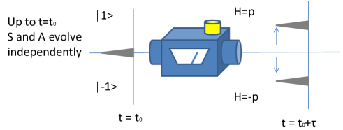
Figure 1: A measurement model with $H_{A}=0$.

Set $H_{S}=0$, $H_{A}=0$ and $V=\sigma_{z}\otimes p$, where $p$ represents the momentum operator. As the meter observable we employ $\{\int_{x\geq 0}dx|x\rangle\langle x|,\int_{x<0}dx|x\rangle\langle x|\}$. For an arbitrary time duration $\tau$, if the initial state at time $t=t_{0}$ of the apparatus is prepared in a narrowly-localized state with respect to a position, the accuracy of the measurement of $\sigma_{z}$ can be made arbitrarily high. Therefore, there is no limitation on the time and energy required for this measurement process.

By looking carefully at this model, one may notice that the time duration is given by hand. In this model, the interaction between a system and an apparatus is switched on at $t=t_{0}$ and switched off at $t=t_{0}+\tau$. The dynamics outside this time interval is not discussed. An external observer must put these systems together at $t=t_{0}$, which until then must have been somehow independent. Thus the mechanism initiating this switching-on process is supposed to be outside the quantum model. In this sense, this model is not closed and we need to shift the interface further to include the on-and-off switching process.

In the discussion below, we develop a general measurement process that also treats this switching-on (and off) mechanism quantum mechanically. In some situations, roughly speaking, we shift the quantum-classical interface so that the quantum side includes the experimenter who controls the apparatus. In the next section we give a mathematically rigorous formulation of the timing device that switches on a perturbation.

III Apparatus as a switching device for an interaction

As stated above, we investigate an apparatus that works not only as an information extractor but also as a switching device for an interaction (perturbation). To do so, in this section, we study a formulation of the latter condition and derive some results. We consider an apparatus that works as a timing device to switch on an interaction at a certain time after $t=t_{0}$. Thus, we assume that at time $t=t_{0}$ the state of the total system is a product state. The apparatus is specified by the Hilbert space $\mathcal{K}$, Hamiltonian $H_{A}$ and a state $\sigma(t_{0})$ at time $t=t_{0}$.

Let us first assume that the apparatus is perfectly isolated and has no interaction with the system. Then the time evolution is described by a von Neumann equation determined by an apparatus Hamiltonian $H_{A}$ which acts only on $\mathcal{K}$. For an arbitrary time $t\in\mathbb{R}$, the state at time $t$ is written as $\sigma(t)=e^{-i\frac{H_{A}(t-t_{0})}{\hbar}}\sigma(t_{0})e^{i\frac{H_{A}(t-t_{0})}{\hbar}}$.

Next, we consider an interaction between the system and apparatus. We denote the Hilbert space of the system by $\mathcal{H}$. The individual dynamics of the system is governed by the Hamiltonian $H_{S}$ defined on $\mathcal{H}$. Thus the total Hamiltonian has three parts, $H=H_{S}+H_{A}+V$, where $V$ is the interaction Hamiltonian that acts on the tensor product $\mathcal{H}\otimes\mathcal{K}$. The time evolution of a state $\Theta(t)$ (a density operator) over the composite system is described by the corresponding von Neumann equation,

$$i\hbar\frac{d}{dt}\Theta(t)=[H,\Theta(t)].$$

Let us consider conditions for $H_{A}$, $V$ and a state of the apparatus to describe a timing device. They must satisfy the following general conditions that represent the capability to switch on the interaction at a certain time. The apparatus evolves freely up to time $t=t_{0}$ and then switches on an interaction with the system at some time after $t=t_{0}$. Thus, the state of the apparatus should be decoupled from that of the system until time $t=t_{0}$. The time evolution of the state is determined entirely once the state at a certain time is given. We impose the following condition on the dynamics and the state at time $t=t_{0}$:

Condition 1.

(No interaction up to time $t=t_{0}$) An apparatus (specified by $H_{A}$, $V$ and a state $\sigma(t_{0})$ at time $t=t_{0}$) satisfies the no interaction condition up to time $t=t_{0}$ if for any $t\leq t_{0}$ and for any state $\rho$ of the system,

$$[V,\rho\otimes\sigma(t)]=0$$ (1)

holds, where $\sigma(t):=e^{-i\frac{H_{A}(t-t_{0})}{\hbar}}\sigma(t_{0})e^{i\frac{H_{A}(t-t_{0})}{\hbar}}$.

We emphasize that in Condition 1, the left-hand side of (1) must be vanishing for any $\rho$. This condition implies that only after the apparatus reaches $\sigma(t_{0})$, does $V$ induce the apparatus and the system to interact. In fact the following lemma shows that these conditions are equivalent.

Lemma 1.

Condition 1 is satisfied if and only if for any state $\rho$ of the system and $t\leq t_{0}$,

$$e^{-i\frac{H(t-t_{0})}{\hbar}}(\rho\otimes\sigma(t_{0}))e^{i\frac{H(t-t_{0})}{\hbar}}=\rho(t)\otimes\sigma(t)$$ (2)

holds, where $\rho(t)$ is defined by $\rho(t)=e^{-i\frac{H_{S}(t-t_{0})}{\hbar}}\rho e^{i\frac{H_{S}(t-t_{0})}{\hbar}}.$

Proof.

“If part”: We differentiate by $t$,

$$e^{-i\frac{H(t-t_{0})}{\hbar}}(\rho\otimes\sigma(t_{0}))e^{i\frac{H(t-t_{0})}{\hbar}}=\rho(t)\otimes\sigma(t)$$

to obtain

$$[H,e^{-i\frac{H(t-t_{0})}{\hbar}}(\rho\otimes\sigma(t_{0}))e^{i\frac{H(t-t_{0})}{\hbar}}]=[H_{S}+H_{A},\rho(t)\otimes\sigma(t)].$$

As the left-hand side is written as $[H_{S}+H_{A}+V,\rho(t)\otimes\sigma(t)]$, we obtain $[V,\rho(t)\otimes\sigma(t)]=0$. As $\rho$ is arbitrary, we obtain Condition 1.
“Only if” part: It holds that for $t\leq t_{0}$,

$$i\hbar\frac{d}{dt}\rho(t)\otimes\sigma(t) = [H_{S}+H_{A},\rho(t)\otimes\sigma(t)]$$

$$= [H,\rho(t)\otimes\sigma(t)],$$

where we used (1) for $\rho(t)$. Thus we conclude that $\rho(t)\otimes\sigma(t)$ satisfies the von Neumann equation whose integration is (2). ∎

This condition ensures that if once the state at an arbitrary time $t_{1}<t_{0}$ is prepared as $\rho(t_{1})\otimes\sigma(t_{1})$, the composite system evolves independently up to time $t=t_{0}$.

Lemma 2.

If Condition 1 is satisfied and at a certain time $t_{1}\leq t_{0}$ the state has a product form $\Theta(t_{1})=\rho(t_{1})\otimes\sigma(t_{1})$; then the state $\Theta(t)$ at any time $t\leq t_{0}$ becomes the product state;

$$\Theta(t)=\rho(t)\otimes\sigma(t),$$

where $\rho(t)=e^{-i\frac{H_{S}}{\hbar}(t-t_{1})}\rho(t_{1})e^{i\frac{H_{S}}{\hbar}(t-t_{1})}$.

Proof.

It follows immediately from Lemma 1. ∎

It is easy to see that a trivial interaction $V=0$ satisfies Condition 1. The following condition is imposed to avoid such a trivial interaction.

Condition 2.

(Non-triviality condition) An apparatus satisfies the non-triviality condition if there exists a state $\rho$ and a time $t>t_{0}$ such that

$$[V,e^{-i\frac{H(t-t_{0})}{\hbar}}(\rho\otimes\sigma(t_{0}))e^{i\frac{H(t-t_{0})}{\hbar}}]\neq 0.$$

Note that this condition is rather weak. It still allows the existence of $\rho$ such that $V$ acts trivially on $\rho(t)\otimes\sigma(t)$ for any $t\in\mathbb{R}$. In addition, this condition does not specify exactly the switching time of the perturbation as $t=t_{0}$. It only requires the existence of the moment $(t>t_{0})$ at which the perturbation does not vanish.

It is possible to further impose a condition on the switching-off process of an interaction.

Condition 3.

(Switching-off time condition) An apparatus satisfies the switching-off time condition if there exists a time $t_{1}>t_{0}$ called a switching off time such that for any $t\geq t_{1}$ and for any state $\rho$ of the system,

$$[V,e^{-i\frac{H(t-t_{0})}{\hbar}}(\rho\otimes\sigma(t_{0}))e^{i\frac{H(t-t_{0})}{\hbar}}]=0$$ (3)

holds.

One may consider a weaker definition for the switching-off time that depends on an initial state of the system. However, in this paper we do not use the switching-off condition.

Example 1.

Suppose that an apparatus is described by $\mathcal{K}=L^{2}(\mathbb{R})$ and $H_{A}=p:=-i\hbar\frac{d}{dx}$. It is coupled with a system described by $\mathcal{H}=\mathbb{C}^{2}$ with orthonormal basis $\{|0\rangle,|1\rangle\}$ and a trivial Hamiltonian $H_{S}=0$. The interaction term is introduced as $V=\sigma_{z}\otimes g(q)$, where $\sigma_{z}=|1\rangle\langle 1|-|0\rangle\langle 0|$ and $g$ is a nonvanishing real function whose support is included in $(0,\Delta)$ for some $\Delta>0$. In the position representation $|\phi(0)\rangle$ is supposed to be strictly localized in the negative real line. That is, the support of $\phi(t=0,x):=\langle x|\phi(0)\rangle$ is included in $(-\delta,0)$ for some $\delta>0$. The freely evolved state of the apparatus can be written as $\phi(t,x)=\phi(0,x-t)$, which has support in $(-\delta+t,t)$. It is easy to see that this system-plus-apparatus satisfies Condition 1.

Let us consider the time evolution of the state denoted by $|\Omega(0)\rangle\otimes|\phi(0)\rangle$. For $|\Omega(0)\rangle=|0\rangle$, while the state of the system remains $|0\rangle$, the state of the apparatus is affected by the interaction. We denote the whole state at time $t$ by $|0\rangle\otimes|\phi^{0}(t)\rangle$. It can be shown that at time $t$, the state of the apparatus $|\phi^{0}(t)\rangle$ becomes $\phi^{0}(t,x)=e^{-\frac{i}{\hbar}\int^{x}_{0}dx^{\prime}g(x^{\prime})}\phi(t,x)$ in the position representation. On the other hand, for $|\Omega(0)\rangle=|1\rangle$, while the state of the system remains $|1\rangle$, the state $|\phi^{1}(t)\rangle$ of the apparatus at time $t$ becomes $\phi^{1}(t,x)=e^{\frac{i}{\hbar}\int^{x}_{0}dx^{\prime}g(x^{\prime})}\phi(t,x)$ in the position representation. Thus, for a general initial state $|\Omega(0)\rangle=c_{0}|0\rangle+c_{1}|1\rangle$, the state of the total system evolves as

$$|\Phi(t)\rangle=c_{0}|0\rangle\otimes|\phi^{0}(t)\rangle+c_{1}|1\rangle\otimes|\phi^{1}(t)\rangle,$$

which coincides with an unperturbed (freely evolved) state up to time $t=0$. Thus it satisfies Condition 1. The state of the system evolves as

$$\rho(t)=|c_{0}|^{2}|0\rangle\langle 0|+|c_{1}|^{2}|1\rangle\langle 1|+c_{0}\overline{c_{1}}|0\rangle\langle 1|\langle\phi^{1}(t)|\phi^{0}(t)\rangle+c_{1}\overline{c_{0}}|1\rangle\langle 0|\langle\phi^{0}(t)|\phi^{1}(t)\rangle,$$

which does not agree, in general, with the freely evolved state

$$\rho^{0}(t)=|c_{0}|^{2}|0\rangle\langle 0|+|c_{1}|^{2}|1\rangle\langle 1|+c_{0}\overline{c_{1}}|0\rangle\langle 1|+c_{1}\overline{c_{0}}|1\rangle\langle 0|$$

for $t>0$. Thus Condition 2 is also satisfied. In addition, we put $\tau=\Delta+\delta$. Taking into account the support of $\phi(t,x)$, we obtain for $t>\tau$,

$$\phi^{0}(t,x)=e^{-\frac{i}{\hbar}\int^{\Delta}_{0}dx^{\prime}g(x^{\prime})}\phi(t,x)$$

$$\phi^{1}(t,x)=e^{\frac{i}{\hbar}\int^{\Delta}_{0}dx^{\prime}g(x^{\prime})}\phi(t,x).$$

As their supports do not intersect with the support of $g$, Condition 3 is satisfied.

The total Hamiltonian in the above example has unbounded spectrum $\mathbb{R}$. This unboundedness must be satisfied in general.

Theorem 1.

Let us consider a model satisfying both Condition 1 and Condition 2. The spectrum of the total Hamiltonian $H=H_{S}+H_{A}+V$ is two-side unbounded (lower and upper unbounded).

Proof.

Suppose that $H$ is lower bounded. (An upper bounded case can be treated similarly.) By purifying the state $\sigma(t_{0})$ of the apparatus, we can assume the state $\sigma(t_{0})$ to be pure. We denote the purified state by $\sigma(t_{0})=|\phi(t_{0})\rangle\langle\phi(t_{0})|$. On this enlarged system, $H$ also works as a Hamiltonian and is lower bounded. (More precisely we need $H\otimes\mathbf{1}$, where $\mathbf{1}$ acts only on an auxiliary Hilbert space employed for purification.) We denote by $\mathcal{K}$ again the enlarged Hilbert space of the apparatus. For an arbitrary state $|\Omega\rangle\in\mathcal{H}$, we have for $t\leq t_{0}$,

$$[V,e^{-i\frac{H}{\hbar}(t-t_{0})}|\Omega\otimes\phi(t_{0})\rangle\langle\Omega\otimes\phi(t_{0})|e^{i\frac{H}{\hbar}(t-t_{0})}]=0.$$

This implies that for $t\leq t_{0}$ there exists a function $c(t)$ such that

$$Ve^{-i\frac{H}{\hbar}(t-t_{0})}|\Omega\otimes\phi(t_{0})\rangle=c(t)|\Omega\otimes\phi(t_{0})\rangle.$$

As $|\Omega\otimes\phi(t_{0})\rangle$ is normalized we have

$$Ve^{-i\frac{H}{\hbar}(t-t_{0})}|\Omega\otimes\phi(t_{0})\rangle=|\Omega\otimes\phi(t_{0})\rangle\langle\Omega\otimes\phi(t_{0})|Ve^{-i\frac{H}{\hbar}(t-t_{0})}|\Omega\otimes\phi(t_{0})\rangle.$$

For an arbitrary $|\Psi\rangle\in\mathcal{H}\otimes\mathcal{K}$ we now define

$$f_{\Psi,\Omega}(t):=\langle\Psi|\left(Ve^{-i\frac{H}{\hbar}(t-t_{0})}-\langle\Omega\otimes\phi(t_{0})|Ve^{-i\frac{H}{\hbar}(t-t_{0})}|\Omega\otimes\phi(t_{0})\rangle\right)|\Omega\otimes\phi(t_{0})\rangle.$$

This is vanishing for $t\leq t_{0}$. As $H$ is lower bounded, $f_{\Psi,\Omega}(z):=\langle\Psi|\left(Ve^{-i\frac{H_{c}}{\hbar}(z-t_{0})}-\langle\Omega\otimes\phi(t_{0})|Ve^{-i\frac{H}{\hbar}(z-t_{0})}|\Omega\otimes\phi(t_{0})\rangle\right)|\Omega\otimes\phi(0)\rangle$ can be defined for $Im(z)\leq 0$ and is analytic for $Im(z)<0$ Hergerfeldt . The Schwarz reflection principle Ahlforsbook implies that $f_{\Psi,\Omega}$ can be extended to an analytic function on $\mathbb{C}\setminus\{s|s>0\}$. Because $f_{\Psi,\Omega}(t)=0$ on $t\leq t_{0}$, it follows that $f_{\Psi,\Omega}(t)=0$ for $t\in\mathbb{R}$. That is, for all $t\in\mathbb{R}$,

$$Ve^{-i\frac{H}{\hbar}(t-t_{0})}|\Omega\otimes\phi(t_{0})\rangle=|\Omega\otimes\phi(t_{0})\rangle\langle\Omega\otimes\phi(t_{0})|Ve^{-i\frac{H}{\hbar}(t-t_{0})}|\Omega\otimes\phi(t_{0})\rangle$$

holds. This contradicts Condition 2. ∎

The unbounded character of the total Hamiltonian implies that the total system is an unstable system or an infinite system. In the latter case, the Hamiltonian is the generator of time evolution referring to a state through the GNS representation Haagbook . We present a more “physical” example whose Hamiltonian is bounded from below. In this example, the conditions are relaxed to yield small errors.

Example 2.

Suppose that an apparatus is described by a one-particle Hilbert space $\mathcal{K}=L^{2}(\mathbb{R})$. We consider a “real” single particle which has Hamiltonian $H_{A}=\frac{p^{2}}{2m}=-\frac{\hbar^{2}}{2m}\frac{d^{2}}{dx^{2}}$ with a particle mass $m>0$. This $H_{A}$ is lower-bounded. We set $t_{0}=0$ and some large $T\gg 0$. We set $|\phi(-T)\rangle$ in its position representation as

$$\phi(-T,x)=\frac{1}{\pi^{1/4}\sqrt{\sigma}}\exp\left(ik(x-x_{0})-\frac{(x-x_{0})^{2}}{2\sigma^{2}}\right),$$

where $k>0$ and $x_{0}$ is chosen to satisfy $-x_{0}=\frac{\hbar k}{m}(T+\Delta)$ for some fixed $\Delta>0$. Then it evolves according to the free Hamiltonian $H_{A}=\frac{p^{2}}{2m}$ as

$$\phi(s-T,x)=\frac{1}{\pi^{1/4}\sqrt{\sigma}\left(1+\frac{is\hbar}{\sigma^{2}m}\right)}\exp\left(\frac{-\frac{(x-x_{0})^{2}}{2\sigma^{2}}+ik(x-x_{0})-\frac{is\hbar k^{2}}{2m}}{1+\frac{is\hbar}{\sigma^{2}m}}\right).$$

It gives rise to the probability distribution, for $v_{g}:=\hbar k/m$,

$$|\phi(s-T,x)|^{2}=\frac{\pi^{1/2}}{\sigma\left(1+\frac{s^{2}\hbar^{2}}{\sigma^{4}m^{2}}\right)}\exp\left(\frac{-\frac{1}{\sigma^{2}}\left(x-x_{0}-v_{g}s\right)^{2}}{1+\frac{s^{2}\hbar^{2}}{\sigma^{4}m^{2}}}\right),$$

which gives an expectation and variance of $q$ as

$$\langle q(s-T)\rangle = x_{0}+v_{g}s$$ (4)

$$\Delta q(s-T) := \sqrt{\langle q(s-T)^{2}\rangle-\langle q(s-T)\rangle^{2}}=\sigma\left(1+\frac{\hbar^{2}s^{2}}{\sigma^{4}m^{2}}\right)^{1/2}.$$ (5)

Let us consider a composite system $\mathcal{H}\otimes\mathcal{K}$, where $\mathcal{H}$ is a Hilbert space with a Hamiltonian $H_{S}$. The total Hamiltonian is assumed to have a form,

$$H=H_{S}+H_{A}+B\otimes V(q),$$

where $B$ is a self-adjoint operator and $suppV(\cdot)\subset(0,\infty)$. One can see that for sufficiently large $t$ the interaction term gives a non-trivial effect. In the following we show that up to time $t_{0}=0$ the states evolve almost freely. We estimate, for $s\leq T$,

$$\|e^{-i\frac{Hs}{\hbar}}|\xi\otimes\phi(-T)\rangle-|\xi(t)\otimes\phi(s-T)\rangle\| = \||\xi\otimes\phi(-T)\rangle-W(s)|\xi\otimes\phi(-T)\rangle\|$$

$$\leq \int^{s}_{0}dt\left\|\frac{d}{dt}W(t)|\xi\otimes\phi(-T)\rangle\right\|,$$

where $W(t)=e^{i\frac{Ht}{\hbar}}e^{-i\frac{H_{0}t}{\hbar}}$ with $H_{0}=H_{S}+H_{A}$. We obtain

$$\frac{d}{dt}W(t)|\xi\otimes\phi(-T)\rangle=\frac{i}{\hbar}W(t)e^{i\frac{H_{0}t}{\hbar}}(B\otimes V(q))e^{-i\frac{H_{0}t}{\hbar}}|\xi\otimes\phi(-T)\rangle.$$

Defining a projection $P_{\geq}$ by $(P_{\geq}\psi)(x)=\left\{\begin{array}[]{cc}\psi(x)&(x\geq 0)\\ 0&(x<0)\\ \end{array}\right.$, we have

$$e^{i\frac{H_{0}t}{\hbar}}(B\otimes V(q))e^{-i\frac{H_{0}t}{\hbar}}|\xi\otimes\phi(-T)\rangle=e^{i\frac{H_{0}t}{\hbar}}(B\otimes V(q))(\mathbf{1}\otimes P_{\geq})e^{-i\frac{H_{0}t}{\hbar}}|\xi\otimes\phi(-T)\rangle,$$

and

$$\|e^{i\frac{H_{0}t}{\hbar}}(B\otimes V(q))e^{-i\frac{H_{0}t}{\hbar}}|\xi\otimes\phi(-T)\rangle\|\leq\|B\otimes V(q)\|\|(\mathbf{1}\otimes P_{\geq})e^{-i\frac{H_{0}t}{\hbar}}|\xi\otimes\phi(-T)\rangle\|$$

$$= \|B\|\|V(q)\|\|P_{\geq}e^{-\frac{H_{A}t}{\hbar}}|\phi(-T)\rangle\|.$$

We can estimate $\|P_{\geq}|\phi(t-T)\rangle\|^{2}=\int^{\infty}_{0}|\phi(t-T,x)|^{2}$. We use (4), (5) and the Chebyshev inequality to give, for $t\leq T$,

$$\|P_{\geq}|\phi(t-T)\rangle\|^{2}\leq\frac{\sigma^{2}\left(1+\frac{\hbar^{2}t^{2}}{\sigma^{4}m^{2}}\right)}{(x_{0}+v_{g}t)^{2}}\leq\frac{\sigma^{2}\left(1+\frac{\hbar^{2}t^{2}}{\sigma^{4}m^{2}}\right)}{(v_{g}\Delta)^{2}},$$

which can be made arbitrarily small as $k\to\infty$. Thus, we have

$$\|e^{-i\frac{Hs}{\hbar}}|\xi\otimes\phi(-T)\rangle-|\xi(t)\otimes\phi(s-T)\rangle\|\leq\|B\|\|V(q)\|\frac{\sigma}{v_{g}\Delta}\left(s+\frac{\hbar^{2}}{3\sigma^{4}m^{2}}s^{3}\right),$$

which can be arbitrary small for $k\to\infty$. Thus, up to time $t_{0}=0$, the interaction can be made negligibly small.

IV Energy-Time Uncertainty Relation I: Energy of Apparatus

In this section we investigate how much energy is required to realize a measurement process satisfying Condition 1. More precisely, we study the energy fluctuation $\Delta H_{A}$ of the apparatus Hamiltonian required for a measurement within a measurement time duration $\tau$, and derive the energy-time uncertainty relation between them.

We treat a closed composite system consisting of a system and a measuring apparatus whose total Hilbert space is $\mathcal{H}\otimes\mathcal{K}$. The dynamics is governed by a total Hamiltonian $H=H_{S}+H_{A}+V$, where $H_{S}$ (respectively $H_{A}$) is the system Hamiltonian acting on $hi$ (resp. $\mathcal{K}$) and $V$ is the interaction. The apparatus must be large enough to include the switching-on process. That is, the model with an “initial” state $\sigma(t_{0})$ of the apparatus at time $t=t_{0}$ satisfies Condition 1. In addition, the model is assumed to describe a measurement process of a sharp observable i.e., a PVM $\mathsf{P}=\{\mathsf{P}_{n}\}_{n\in\Omega_{\mathsf{P}}}$ with a measurement time duration $\tau>0$. That is, there exists a POVM $\mathsf{E}=\{\mathsf{E}_{n}\}_{n\in\Omega_{\mathsf{P}}}$ acting on $\mathcal{K}$ such that it holds that for an arbitrary state $\rho$ of the system,

$$\mbox{tr}[\rho\mathsf{P}_{n}]=\mbox{tr}[e^{-i\frac{H}{\hbar}\tau}(\rho\otimes\sigma(t_{0}))e^{i\frac{H}{\hbar}{\tau}}(\mathbf{1}\otimes\mathsf{E}_{n})].$$

Two observations play roles in deriving a result. The first is a so-called information-disturbance trade-off relation in the quantum measurement process. In quantum mechanics, any non-trivial measurement process causes disturbance of quantum states. This property is directly related to the uncertainty relation of joint measurement. In fact, the disturbance caused by a measurement of an observable spoils the subsequent measurements. In particular, a perfectly accurate measurement of an observable implies a complete distortion of the conjugate states. The second observation, which is derived in this section for the first time, is a kind of energy-time uncertainty relation between the energy fluctuation of an apparatus and the time duration required to disturb a state of the system. This relation is proved by applying the Mandelstam-Tamm uncertainty relation to a timing device satisfying Condition 1. Combining these two observations, we derive a trade-off inequality between the time duration of the measurement process and the energy fluctuation of the apparatus.

We begin with the latter problem: how large an energy fluctuation is required to disturb a state. We examine the behavior of states of a system interacting with a timing device. We consider the time evolution of $\Theta_{0}(t_{0}):=\rho(t_{0})\otimes\sigma(t_{0})$, where $\rho(t_{0})$ is a state of the system at time $t=t_{0}$. Its evolved state is denoted by $\Theta_{0}(t)=e^{-i\frac{H}{\hbar}(t-t_{0})}\Theta_{0}(t_{0})e^{i\frac{H}{\hbar}(t-t_{0})}$, and its restricted state on the system is written as $\rho(t):=\mbox{tr}_{\mathcal{K}}\Theta_{0}(t)$, where $\mbox{tr}_{\mathcal{K}}$ represents a partial trace. This state $\rho(t)$ should be compared to the freely evolved (imaginary) state $\rho^{0}(t):=e^{-i\frac{H_{S}}{\hbar}(t-t_{0})}\rho(t_{0})e^{i\frac{H_{S}}{\hbar}(t-t_{0})}$.

We employ a quantity, called fidelity, to quantify the deviation. The fidelity between the two states $\rho_{0}$ and $\rho_{1}$ is defined by $F(\rho_{0},\rho_{1}):=\mbox{tr}(\sqrt{\rho_{0}^{1/2}\rho_{1}\rho_{0}^{1/2}})$. It satisfies $0\leq F(\rho_{0},\rho_{1})\leq 1$, and $F(\rho_{0},\rho_{1})=1$ holds if and only if $\rho_{0}=\rho_{1}$. (See for example, Nielsen .)

Now we consider a timing device which satisfies Condition 1. The energy fluctuation of the apparatus at $t=t_{0}$

$$\Delta H_{A}:=\sqrt{\mbox{tr}[\sigma(t_{0})H_{A}^{2}]-\mbox{tr}[\sigma(t_{0})H_{A}]^{2}}$$

plays a central role in the following theorems. Because up to time $t=t_{0}$ the apparatus evolves only by $H_{A}$, the energy fluctuation is constant for $t\leq t_{0}$. This quantity characterizes the speed of the time evolution for the isolated apparatus. Because of Condition 1, the state of the apparatus evolves up to time $t=t_{0}$ as if it is isolated. Thus $\sigma(t)$, a state of the apparatus for $t\leq t_{0}$, is written as $\sigma(t)=e^{-i\frac{H_{A}}{\hbar}(t-t_{0})}\sigma(t_{0})e^{i\frac{H_{A}}{\hbar}(t-t_{0})}$. The well-known Mandelstam-Tamm time energy uncertainty relation Mandelstam-Tamm ; Busch1 ; BuschTEUR ; Pfeifer states that for any normalized vector $|\phi(t)\rangle=e^{-i\frac{H_{A}}{\hbar}(t-t_{0})}|\phi(t_{0})\rangle\in\mathcal{K}$, their overlap is bounded as

$$|\langle\phi(t)|\phi(t_{0})\rangle|\geq\cos\left(\frac{\Delta H_{A}(t-t_{0})}{\hbar}\right)$$

for $|t-t_{0}|\leq\frac{\pi\hbar}{2\Delta H_{A}}$.

Lemma 3.

For $t$ satisfying $0\leq t_{0}-t\leq\frac{\pi\hbar}{2\Delta H_{s}}$, the fidelity between $\sigma(t)$ and $\sigma(t_{0})$ is bounded as

$$F(\sigma(t),\sigma(t_{0}))\geq\cos\left(\frac{\Delta H_{A}(t-t_{0})}{\hbar}\right).$$ (6)

Proof.

The fidelity is the maximum overlap between the purified states as $F(\sigma(t),\sigma(t_{0}))=\sup|\langle\phi(t)|\phi(t_{0})\rangle|$, and the above inequality can be obtained for the fidelity by using $\Delta H_{A}=\Delta(H_{A}\otimes\mathbf{1})$, where $\Delta(H_{A}\otimes\mathbf{1})$ is the energy fluctuation of the purified state $|\phi(t_{0})\rangle$ of $\sigma(t_{0})$. ∎

The deviation of the perturbed state, measured by the fidelity, can be bounded by the following simple argument.

Theorem 2.

Let us consider a process that satisfies Condition 1. $F(\rho(t),\rho^{0}(t))$ represents the fidelity between $\rho(t)$ and the freely evolved state $\rho^{0}(t)$. It holds that for $0\leq t-t_{0}\leq\frac{\pi\hbar}{2\Delta H_{A}}$,

$$\cos\left(\frac{\Delta H_{A}(t-t_{0})}{\hbar}\right)\leq F(\rho(t),\rho^{0}(t)).$$

Proof.

Let us consider two states $\Theta_{t_{0}}(t_{0})$ and $\Gamma_{t}(t_{0})$ $(0\leq t-t_{0}\leq\frac{\pi\hbar}{2\Delta H_{c}})$ defined by

$$\Theta_{t_{0}}(t_{0}) := \rho(t_{0})\otimes\sigma(t_{0})$$

$$\Gamma_{t}(t_{0}) := \rho(t_{0})\otimes\sigma(t_{0}-(t-t_{0})).$$

These states evolve with the Hamiltonian $H=H_{S}+H_{A}+V$. We denote the states at time $t$ by $\Theta_{t_{0}}(t)$ and $\Gamma_{t}(t)$. Although $\Theta_{t_{0}}(t)$ may have a complicated form, $\Gamma_{t}(t)$ has a simple form as it evolves freely,

$$\Gamma_{t}(t)=\rho^{0}(t)\otimes\sigma(t_{0}),$$

where we used Lemma 2. Because the fidelity between the two states is invariant under unitary evolution Nielsen , it holds that

$$F(\Theta_{t_{0}}(t_{0}),\Gamma_{t}(t_{0}))=F(\Theta_{t_{0}}(t),\Gamma_{t}(t)).$$

The left-hand side of the above equation becomes

$$F(\Theta_{t_{0}}(t_{0}),\Gamma_{t}(t_{0}))=F(\sigma(t_{0}),\sigma(t_{0}-(t-t_{0})),$$

and the right-hand side is bounded as

$$F(\Theta_{t_{0}}(t),\Gamma_{t}(t))\leq F(\rho(t),\rho^{0}(t)),$$

where we utilized the fact that the fidelity decreases for restricted states Nielsen . Thus it holds that

$$F(\sigma(t_{0}),\sigma(t_{0}-(t-t_{0}))\leq F(\rho(t),\rho^{0}(t)).$$

The left-hand side of this inequality represents the speed of time evolution of the apparatus and is bounded as (6). This concludes the proof. ∎

Now, we use an information-disturbance trade-off relation to estimate the size of the perturbation caused by a measurement. We study a process in which a sharp observable is perfectly measured. The following is our main result:

Theorem 3.

Let us consider a measurement process of a sharp observable $\mathsf{P}=\{\mathsf{P}_{n}\}$ that satisfies Condition 1. Its measurement time duration $\tau$ and energy fluctuation of an apparatus $\Delta H_{A}$ must satisfy

$$\tau\cdot\Delta H_{A}\geq\frac{\pi\hbar}{4}.$$

Proof.

We consider the dynamics from time $t=t_{0}$ to $t=t_{0}+\tau$. Suppose that $0$ and $1$ are possible outcomes. We consider two states $|0\rangle$ and $|1\rangle$ satisfying $P_{0}|0\rangle=|0\rangle$, $P_{1}|0\rangle=0$, $P_{1}|1\rangle=|1\rangle$, and $P_{0}|1\rangle=0$. We suppose that for a time duration $\tau$ an initial state (at time $t_{0}$) $|0\rangle\langle 0|\otimes\sigma(t_{0})$ evolves to $\Theta_{0}$, and an initial state $|1\rangle\langle 1|\otimes\sigma(t_{0})$ evolves to $\Theta_{1}$. In a perfectly accurate measurement process, their restricted states to the apparatus, $\mbox{tr}_{\mathcal{H}}[\Theta_{0}]$ and $\mbox{tr}_{\mathcal{H}}[\Theta_{1}]$, are perfectly distinguishable. We can show that this dynamics spoils completely the possibility to measure its “conjugate” observable afterwards. That is, if we define $|\pm\rangle=\frac{1}{\sqrt{2}}(|0\rangle\pm|1\rangle)$, initial states $|\pm\rangle\langle\pm|\otimes\sigma(t_{0})$ evolve to states whose restriction to the system coincide. We follow the derivation given by Janssens and Maassen Janssens . The states to be compared are $\mbox{tr}_{A}[e^{-i\frac{H}{\hbar}\tau}(|\pm\rangle\langle\pm|\otimes\sigma(t_{0}))e^{i\frac{H}{\hbar}\tau}]$. For an arbitrary operator $\mathsf{A}$ on the system, it holds that

$$|\mbox{tr}[e^{-i\frac{H}{\hbar}\tau}((|+\rangle\langle+|-|-\rangle\langle-|)\otimes\sigma(t_{0}))e^{i\frac{H}{\hbar}\tau}(\mathsf{A}\otimes\mathbf{1})] \leq 2|\mbox{tr}[e^{-i\frac{H}{\hbar}\tau}(|1\rangle\langle 0|\otimes\sigma(t_{0}))e^{i\frac{H}{\hbar}\tau}(\mathsf{A}\otimes\mathbf{1})]|$$ (7)

$$\leq 2\sum_{n}|\mbox{tr}[e^{-i\frac{H}{\hbar}\tau}(|1\rangle\langle 0|\otimes\sigma(t_{0}))e^{i\frac{H}{\hbar}\tau}(\mathsf{A}\otimes\mathsf{E}_{n})]|$$

$$= 2\sum_{n}|\langle 0\otimes\phi(t_{0})|e^{i\frac{H}{\hbar}\tau}(\mathsf{A}\otimes\mathsf{E}_{n}\otimes\mathbf{1})e^{-i\frac{H}{\hbar}\tau}|1\otimes\phi(t_{0})\rangle|,$$

where $|\phi(t_{0})\rangle$ is a purified vector of $\sigma(t_{0})$. By using the Cauchy-Schwarz inequality, we obtain

$$(\ref{tochuu1}) \leq 2\|\mathsf{A}\|\sum_{n}\langle 0\otimes\phi(t_{0})|e^{i\frac{H}{\hbar}\tau}(\mathbf{1}\otimes\mathsf{E}_{n}\otimes\mathbf{1})e^{-i\frac{H}{\hbar}\tau}|0\otimes\phi(t_{0})\rangle^{1/2}\langle 1\otimes\phi(t_{0})|e^{i\frac{H}{\hbar}\tau}(\mathbf{1}\otimes\mathsf{E}_{n}\otimes\mathbf{1})e^{-i\frac{H}{\hbar}\tau}|1\otimes\phi(t_{0})\rangle^{1/2}$$

$$= 2\|\mathsf{A}\|\sum_{n}\delta_{n0}\delta_{n1}=0.$$

Thus the states $|+\rangle\langle+|\otimes\sigma(t_{0})$ and $|-\rangle\langle-|\otimes\sigma(t_{0})$ evolve into states whose restriction to the system is an identical state $\rho$. One can conclude that at least one of the states $|\pm\rangle$ is perturbed. To estimate the magnitude of this perturbation we consider unitary evolution governed by the Hamiltonian $H_{S}$. In time $\tau$, this “unperturbed” dynamics changes $|\pm\rangle$ to a pair of orthogonal states $|\pm^{\prime}\rangle$ of the system. We estimate $F(\rho,|+^{\prime}\rangle\langle+^{\prime}|)$ and $F(\rho,|-^{\prime}\rangle\langle-^{\prime}|)$. As $|\pm^{\prime}\rangle$ are orthogonal, we have

$$F(\rho,|+^{\prime}\rangle\langle+^{\prime}|)^{2}+F(\rho,|-^{\prime}\rangle\langle-^{\prime}|)^{2} = \langle+^{\prime}|\rho|+^{\prime}\rangle+\langle-^{\prime}|\rho|-^{\prime}\rangle$$

$$\leq \mbox{tr}[\rho]=1.$$

Thus we can conclude

$$\min\{F(\rho,|+^{\prime}\rangle\langle+^{\prime}|),F(\rho,|-^{\prime}\rangle\langle-^{\prime}|)\}\leq\frac{1}{\sqrt{2}}.$$

We assume $F(\rho,|+^{\prime}\rangle\langle+^{\prime}|)\leq\frac{1}{\sqrt{2}}$. Combining it with Theorem 2 by putting $\rho(t_{0})=|+\rangle\langle+|$, we obtain

$$\cos\left(\frac{\tau\Delta H_{A}}{\hbar}\right)\leq\frac{1}{\sqrt{2}}.$$

This ends the proof. ∎

The above theorem can be easily extended to obtain the following:

Proposition 1.

Let us consider a measurement process satisfying Condition 1 of a sharp observable $\mathsf{P}$ that has at least $N$ outcomes. The measurement time duration $\tau$ and the fluctuation of the apparatus Hamiltonian $\Delta H_{A}$ satisfy

$$\cos\left(\frac{\tau\Delta H_{A}}{\hbar}\right)\leq\frac{1}{\sqrt{N}}.$$

Proof.

We can assume that PVM $\mathsf{P}$ has the elements $\{\mathsf{P}_{0},\mathsf{P}_{1},\ldots,\mathsf{P}_{N-1}\}$ that have eigenvectors $\{|n\rangle\}_{n=0,1,\ldots,N-1}$ satisfying $\mathsf{P}_{n}|n\rangle=|n\rangle$. Then one can show that states $|\tilde{k}\rangle:=\frac{1}{\sqrt{N}}\sum_{n}e^{i\frac{2\pi kn}{N}}|n\rangle$ evolve into states whose restrictions to the system coincide. In fact, for an arbitrary operator $\mathsf{A}$ on the system, it holds that for $m\neq l$,

$$|\mbox{tr}[e^{-i\frac{H}{\hbar}\tau}(|\tilde{m}\rangle\langle\tilde{m}|-|\tilde{l}\rangle\langle\tilde{l}|\otimes\sigma(t_{0}))e^{i\frac{H}{\hbar}\tau}(\mathsf{A}\otimes\mathbf{1})]\leq\frac{1}{N}\sum_{n\neq n^{\prime}}|\langle n\otimes\phi(t_{0})|e^{i\frac{H}{\hbar}\tau}(\mathsf{A}\otimes\mathbf{1})e^{-i\frac{H}{\hbar}\tau}|n^{\prime}\otimes\phi(t_{0})\rangle|,$$

where $|\phi(t_{0})\rangle$ is a purified state of $\sigma(t_{0})$. The argument employed above bounds the right hand side of this inequality by zero.

Let us denote this identical state at time $t=t_{0}+\tau$ on the system by $\rho$. We denote the states obtained by unperturbed (free) time evolution by $\{|\tilde{k}^{\prime}\rangle\}$, which are orthonormal. Now we have

$$\sum_{k=0}^{N-1}F(\rho,|\tilde{k}^{\prime}\rangle\langle\tilde{k}^{\prime}|)^{2}\leq\mbox{tr}[\rho]=1.$$

Thus $min_{k}F(\rho,|\tilde{k}^{\prime}\rangle\langle\tilde{k}^{\prime}|)\leq\frac{1}{\sqrt{N}}$ is obtained. This ends the proof. ∎

Letting $N$ go to $\infty$, we obtain the following:

Corollary 1.

Let us consider a measurement process satisfying Condition 1 of a sharp observable that has infinitely many outcomes. The measurement time duration $\tau$ and the fluctuation of the apparatus Hamiltonian $\Delta H_{A}$ must satisfy

$$\tau\cdot\Delta H_{A}\geq\frac{\pi\hbar}{2}.$$

As $\Delta H_{A}$ can be infinite for some states, it is instructive to derive a similar trade-off relation for other quantities characterizing energy indefiniteness. For $0<\alpha\leq 1$, the overall width $\Delta_{\alpha}f$ of a distribution function $f$ on $\mathbb{R}$ is defined as the width of the smallest interval $I$ such that

$$\int_{I}dxf(x)\geq\alpha.$$

This quantity has its own corresponding energy-time uncertainty relation Uffink . A closed system with a Hamiltonian $H$ is considered. Let $\tau_{\beta}$ be the minimal time it takes for a state $|\psi(0)\rangle$ to evolve to a state $|\psi(t)\rangle$ such that

$$|\langle\psi(0)|\psi(t)\rangle|\leq\beta.$$

Then one can show, for $\beta\leq 2\alpha-1$,

$$\tau_{\beta}\cdot\Delta_{\alpha}(H)\geq 2\hbar\arccos\frac{\beta+1-\alpha}{\alpha},$$

where $\Delta_{\alpha}(H)$ is the overall width of a distribution function $f(E)$ defined by $\langle\psi(0)|E(dE)|\psi(0)\rangle=f(E)dE$, where $E(dE)$ is a spectral measure of $H$.

This inequality is employed to derive another version of the above result. The proof is given in the Appendix A.

Theorem 4.

Let $\tau$ be a measurement duration. For any $\alpha$ with $\alpha\geq\frac{1}{2}\left(1+\frac{1}{\sqrt{2}}\right)$, it holds that

$$\tau\cdot\Delta_{\alpha}(H)\geq 2\hbar\arccos\frac{\frac{1}{\sqrt{2}}+1-\alpha}{\alpha}.$$

It is interesting to extend the results to measurements with errors. Let us consider again a sharp observable $\mathsf{P}=\{\mathsf{P}_{n}\}$. For an initial state $\rho_{n}$ with $\mathsf{P}_{n}\rho_{n}\mathsf{P}_{n}=\mathsf{P}_{n}$, an imperfect measurement allows errors. That is, there may exist $\rho_{n}$ and $m$ such that $Prob(m|\rho_{n}):=\mbox{tr}[e^{-i\frac{H\tau}{\hbar}}(\rho_{n}\otimes\sigma(t_{0}))e^{i\frac{H\tau}{\hbar}}(\mathbf{1}\otimes\mathsf{E}_{n})]\neq\delta_{nm}$ holds. We introduce $P_{error}$ by

$$P_{error}:=\sup_{n}\sup_{\rho_{n}:\mathsf{P}_{n}\rho_{n}\mathsf{P}_{n}=\rho_{n}}(1-P(n|\rho_{n}))$$

which represents the worst case error probability.

Theorem 5.

Let us consider a measurement process satisfying Condition 1 of a sharp observable $\mathsf{P}=\{\mathsf{P}_{n}\}$ with the worst case error probability $P_{error}$. Its measurement time duration $\tau$ and energy fluctuation of an apparatus $\Delta H_{A}$ satisfies

$$\cos\left(\frac{\tau\Delta H_{A}}{\hbar}\right)\leq\sqrt{\frac{1+6\sqrt{P_{error}}}{2}}.$$

The proof is given in Appendix B.

As mentioned, the uncertainty relation for joint measurement, or the information-disturbance relation, plays a crucial role in our proof. While the quantitative relation given by Janssens and Maassen was employed here, other quantitative relations MiHeisenberg ; MiJMP ; HeMi ought to be applicable. It would be interesting to compare the corresponding energy-time uncertainty relations.

Example 3.

Let us consider an apparatus consisting of a particle in a two-dimensional $xz-$plane. Its Hilbert space is written as $\mathcal{K}=L^{2}(\mathbb{R}^{2})$. We denote by $(q_{x},p_{x},q_{z},p_{z})$ position and momentum operators of their corresponding subscripts. We set an apparatus Hamiltonian $H_{A}$ as

$$H_{A}=p_{x}.$$

We consider a qubit (spin-$1/2$ degree of freedom) as a system whose self Hamiltonian $H_{S}$ is vanishing. Thus a total Hilbert space is written as $\mathcal{H}_{T}=\mathcal{H}\otimes\mathcal{K}=\mathbb{C}^{2}\otimes L^{2}(\mathbb{R}^{2})$. We study a time evolution determined by the total Hamiltonian,

$$H=V+H_{A}=\sigma_{z}g(q_{x})p_{z}+p_{x},$$

where $g$ is a nonnegative smooth function whose support is in $(0,\delta)$ with $\delta>0$. We set an initial state (at time $t=0$) of the apparatus in the position representation as

$$\phi(t=0,x,z)=\langle x,z|\phi(0)\rangle=\xi(x)\eta(z),$$

where $\xi$ is a smooth real function satisfying $\mbox{supp}\xi\subset(-\Delta,0)$ for some $\Delta>0$ and $\eta$ is a smooth function with $\eta(-z)=\eta(z)$ and $\mbox{supp}\eta\subset(-\epsilon,\epsilon)$ for some $\epsilon>0$. We set $\tau:=\delta+\Delta$ and assume that $\epsilon>0$ is small enough to satisfy

$$\epsilon<\int^{\tau}_{0}dtg(t).$$

It is easy to see that this model satisfies Condition 1. Its energy fluctuation up to time $t=0$ is

$$\Delta H_{A}=-\hbar^{2}\int dx\overline{\xi(x)}\frac{d^{2}}{dy^{2}}\xi(x)=\hbar^{2}\int dx\left(\frac{d\xi(x)}{dx}\right)^{2},$$

which becomes finite for sufficiently smooth $\xi$. After a lengthy calculation one can see that if an initial state of the system is $|1\rangle$ (respectively $|-1\rangle$), the probability for $q_{z}>0$ (resp. $q_{z}<0$) at time $t=\tau$ is $1$. Thus this model works as a measurement model of $\sigma_{z}$. If we rescale $\xi$ as, for $C>0$,

$$\xi_{C}(x):=\sqrt{C}\xi(Cx),$$

$\Delta$ is scaled as $\Delta/C$ and thus $\tau$ scales as $\tau/C$. On the other hand, the energy fluctuation $\Delta H_{A}$ is scaled as $C\Delta H_{A}$. Thus this model illustrates the expected energy-time trade-off.

We close this section with a remark on the definition of apparatus. The above example can be regarded as a toy model of the Stern-Gerlach experiment if the qubit is interpreted as the spin degree of freedom of a moving particle. Thus, the apparatus in this model is the position degree of freedom of a particle.

V Energy-Time Uncertainty Relation II: Interaction Strength

In the previous section, we derived a trade-off inequality between the fluctuation of $H_{A}$ and the measurement time duration $\tau$. In this section, we examine the magnitude of interaction $V$ that is required for measurements. In this section Condition 1 is not assumed. The measurement process is described by a total Hamiltonian $H=H_{S}+H_{A}+V$ and the dynamics up to time $t=t_{0}$ is irrelevant. A state of the apparatus $\sigma(t_{0})$ is prepared at time $t=t_{0}$ and a meter observable $\mathsf{E}$ is measured at $t=t_{0}+\tau$. The reason why we do not need conditions for switching-on device to obtain the bound on the interaction is that the interaction Hamiltonian is mainly relevant to the border between the system and the apparatus while the switching-on condition is relevant to the border between the apparatus and the classical system.

Theorem 6.

For a model to describe a measurement process of a PVM, the interaction $V$ must satisfy

$$\|V\|\cdot\tau\geq\frac{\pi}{4}\hbar.$$

Proof.

Again we consider a process exactly measuring a PVM $\mathsf{P}$. Two states $|0\rangle$ and $|1\rangle$ satisfying $P_{0}|0\rangle=|0\rangle$, $P_{1}|1\rangle=|1\rangle$ and $P_{1}|0\rangle=0$, $P_{0}|1\rangle=0$ exist. For a process to distinguish these states exactly, its conjugate states are completely destroyed. That is, if we define $|\pm\rangle=\frac{1}{\sqrt{2}}(|0\rangle+|1\rangle)$, initial states $|\pm\rangle\langle\pm|\otimes\sigma(t_{0})$ are mapped to states that are an identical on the system side. We denote by $\rho$ such a final state on the system. We also denote by $|\pm^{\prime}\rangle$ the states obtained by free evolution without interaction in time $\tau$. We have already shown that

$$\min\{F(\rho,|+^{\prime}\rangle\langle+^{\prime}|),F(\rho,|-^{\prime}\rangle\langle-^{\prime}|)\}\leq\frac{1}{\sqrt{2}}.$$

We assume $F(\rho,|+^{\prime}\rangle\langle+^{\prime}|)\leq\frac{1}{\sqrt{2}}$. The state $\rho$ is written as

$$\rho=\mbox{tr}_{A}[e^{-i\frac{H\tau}{\hbar}}(|+\rangle\langle+|\otimes|\phi(t_{0})\rangle\langle\phi(t_{0})|)e^{i\frac{H\tau}{\hbar}}],$$

where $|\phi(t_{0})\rangle$ is a purified state of $\sigma(t_{0})$ and $\mbox{tr}_{A}$ denotes a partial trace to obtain a restricted state on the system. We introduce a time-evolving vector $|\Phi(t)\rangle:=e^{-i\frac{H(t-t_{0})}{\hbar}}|+\rangle\otimes|\phi(t_{0})\rangle$. On the other hand, $|+^{\prime}\rangle$ satisfies

$$|+^{\prime}\rangle\langle+^{\prime}|\otimes|\phi(t_{0}+\tau)\rangle\langle\phi(t_{0}+\tau)|=e^{-i\frac{H_{0}\tau}{\hbar}}|+\rangle\langle+|\otimes|\phi(t_{0})\rangle\langle\phi(t_{0})|e^{i\frac{H_{0}\tau}{\hbar}},$$

where $H_{0}=H_{S}+H_{A}$. We introduce $|\Phi_{0}(t)\rangle:=e^{-i\frac{H_{0}(t-t_{0})}{\hbar}}|+\rangle\otimes|\phi(t_{0})\rangle$. Since the fidelity does not decrease by the partial trace, the vectors $|\Phi(t)\rangle$ and $|\Phi_{0}(t)\rangle$ satisfy

$$|\langle\Phi_{0}(t_{0}+\tau)|\Phi(t_{0}+\tau)\rangle|\leq\frac{1}{\sqrt{2}}.$$ (8)

Defining $p(t):=\langle\Phi_{0}(t)|\Phi(t)\rangle\langle\Phi(t)|\Phi_{0}(t)\rangle$, we obtain

$$i\hbar\frac{d}{dt}p(t)=\langle\Phi_{0}(t)|[V,|\Phi(t)\rangle\langle\Phi(t)|]\Phi_{0}(t)\rangle.$$

The right-hand side of this equation can be further bounded by the Robertson uncertainty relation as

$$|\langle\Phi_{0}(t)|[V,|\Phi(t)\rangle\langle\Phi(t)|]|\Phi_{0}(t)\rangle|\leq 2(\Delta V)_{t}\sqrt{p(t)-p(t)^{2}},$$

where $(\Delta V)_{t}:=\sqrt{\langle\Phi_{0}(t)|V^{2}|\Phi_{0}(t)\rangle-\langle\Phi_{0}(t)|V|\Phi_{0}(t)\rangle^{2}}\leq\|V\|$. Thus we obtain,

$$\frac{d}{dt}p(t)\leq 2\|V\|\sqrt{p(t)-p(t)^{2}},$$

whose solution shows that

$$p(t)\geq\cos^{2}\left(\frac{\|V\|}{\hbar}(t-t_{0})\right).$$ (9)

By combining (8) and (9), we conclude the proof. ∎

As in the case of energy fluctuation, the right-hand side of the trade-off relation gets larger depending on the number of outcomes. In particular, for observables which have infinitely many outcomes we have the following theorem:

Theorem 7.

Let us consider a measurement model that measures a sharp observable with infinitely many outcomes. Its interaction $V$ must satisfy

$$\|V\|\cdot\tau\geq\frac{\pi}{2}\hbar.$$

Proof.

For an arbitrary $N>0$ we can assume that the PVM to be measured has the elements $\mathsf{P}_{1},\mathsf{P}_{2},\ldots,\mathsf{P}_{N}$ with eigenvectors $\{|n\rangle\}_{n=1,2,\ldots,N}$ satisfying $\mathsf{P}_{n}|n\rangle=|n\rangle$. (If $\mathsf{P}$ has a continuous outcome set, we construct the above elements by discretizing the set.) We can show that the states $|\tilde{k}\rangle:=\frac{1}{\sqrt{N}}\sum_{n}e^{i\frac{2\pi kn}{N}}|n\rangle$ are mapped to an identical state, say $\rho$, on the system. We denote the states obtained by unperturbed (free) time evolution by $\{|\tilde{k}^{\prime}\rangle\}$, which are orthonormalized. Now we have,

$$\sum_{k=1}^{N}F(\rho,|\tilde{k}^{\prime}\rangle\langle\tilde{k}^{\prime}|)^{2}\leq\mbox{tr}[\rho]=1.$$

Thus, $min_{k}F(\rho,|\tilde{k}^{\prime}\rangle\langle\tilde{k}^{\prime}|)\leq\frac{1}{\sqrt{N}}$ is obtained. An argument in the previous proof is applied to show

$$\cos\left(\frac{\|V\|}{\hbar}\tau\right)\leq\frac{1}{\sqrt{N}}.$$

As $N$ was arbitrary, it ends the proof. ∎

In MiyaderaInteraction2011 , a similar bound on the interaction strength was derived that is related to the Hamiltonian $H_{S}$. The relationship of the present work with it will be discussed elsewhere.

VI Spacetime uncertainty relation

As an application of our results on the energy variance required for a measurement, we study the so-called spacetime uncertainty relation. It is believed that spacetime is not a simple continuum at the microscopic scale. A quantum effect is thought to impose some limitation on the microscopic spacetime structure Mead . This limitation has been proposed in various ways including string theory Yoneya . In FDR , Doplicher, Fredenhagen and Roberts gave an ingenious, yet heuristic argument by combining the quantum measurement of local observables with general relativity, as explained below. We may suppose that a spacetime region, say $D$, has its operational meaning if one is able to measure a local observable located at $D$. They argue that one needs to concentrate energy to measure an observable in $D$. If we assume that this energy can be identified with mass, for a sufficiently small $D$ the mass can become too large to avoid black hole formation. As a black hole prevents the extraction of information from the region, the region $D$ looses its operational meaning. (The authors further propose that the spacetime be described by noncommutative geometry.) Their reasoning with respect to the usage of general relativity is heuristic. In addition, the first part of this reasoning still contains an ambiguity. We apply our theorem to strengthen this first part of the energy-time uncertainty relation between apparatus energy fluctuation and measurement time.

We consider a nonrelativistic discrete space $\mathbb{Z}^{d}$. Thus the spacetime is $\mathbb{Z}^{d}\times\mathbb{R}$. There is no apriori reason that the whole part of the apparatus must be located in a small region specified by $D$. That is, one may consider a large apparatus that extends outside the small region to avoid energy concentration. Or, even if the apparatus is localized, it may interact with an infinitely extended environment that has large energy fluctuation. (We investigate the latter possibility below.) This loophole, however, is not applied if the locality of interaction is taken into consideration. Let us consider an apparatus located at the origin $0$ of the lattice (see FIG. 2). Other sites represent the environment. For each $x\in\mathbb{Z}^{d}$ there is a Hilbert space $\mathcal{H}_{x}$ that is not necessarily finite dimensional. The background lattice structure $\mathbb{Z}^{d}$ introduces a natural Euclidean distance between sites denoted by $d(x,y)=\sqrt{\sum_{i}(x_{i}-y_{i})^{2}}$. For each finite region $\Lambda\subset\mathbb{Z}$, we consider a Hilbert space $\otimes_{x\in\Lambda}\mathcal{H}_{x}$ and an observable algebra $\mathfrak{A}(\Lambda)\subset\mathbf{B}(\otimes_{x\in\Lambda}\mathcal{H}_{x})$. (See BR for a precise definition of the mathematical terminology.) For $\Lambda_{1}\subset\Lambda_{2}$, a natural inclusion relation $\mathfrak{A}(\Lambda_{1})\subset\mathfrak{A}(\Lambda_{2})$ is introduced. Thus an arbitrary pair of observables $A_{j}\in\mathfrak{A}(\Lambda_{j})$ $(j=1,2)$ for any disjoint regions $\Lambda_{1}$ and $\Lambda_{2}$ satisfies $[A_{1},A_{2}]=0$. The total observable algebra is defined by $\mathfrak{A}:=\overline{\cup_{\Lambda}\mathfrak{A}(\Lambda)}^{\|\cdot\|}$, where the summation is taken over all finite regions and it is made closed with respect to norm topology. The dynamics is specified by a local Hamiltonian. On each site a self Hamiltonian $h_{x}$ acting only on $\mathcal{H}_{x}$ is defined. The interaction must be local. For simplicity, we assume that the interaction is nearest-neighbor. That is, only for each pair $\{x,y\}$ satisfying $d(x,y)=1$, an interaction $\Phi(\{x,y\})$ that acts on $\mathcal{H}_{x}\otimes\mathcal{H}_{y}$ is non-trivial. For each finite region $\Lambda\subset\mathbb{Z}^{d}$, let $H_{\Lambda}$ denote its “box Hamiltonian” defined by

$$H_{\Lambda}=\sum_{x\in\Lambda}h_{x}+\sum_{\{x,y\}\subset\Lambda}\Phi(x,y).$$

This box Hamiltonian defines the dynamics (in the Heisenberg picture) by $\beta^{\Lambda}_{t}(\mathsf{A})=e^{i\frac{H_{\Lambda}}{\hbar}t}\mathsf{A}e^{-i\frac{H_{\Lambda}}{\hbar}t}$, where $\beta^{\Lambda}_{t}$ is a one-parameter $*$-automorphism group $(t\in\mathbb{R})$. The infinite volume limit on the box converges and defines the dynamics, $\beta_{t}$, by

$$\beta_{t}(\mathsf{A})=\lim_{\Lambda\to\mathbb{Z}^{d}}\beta^{\Lambda}_{t}(\mathsf{A}),$$

where the limit is taken with respect to norm topology. Let us consider a system to be measured. We assume that it interacts only with an apparatus and has a Hilbert space $\mathcal{H}$. Its own dynamics is governed by a system Hamiltonian $H_{S}$, which defines a one parameter group of $*$-automorphism $\gamma_{t}$ by $\gamma_{t}(\mathsf{B})=e^{i\frac{H_{S}}{\hbar}t}\mathsf{B}e^{i\frac{H_{S}}{\hbar}t}$ for $\mathsf{B}\in\mathbb{B}(\mathcal{H})$. The interaction is given by an interaction Hamiltonian $V$ acting only on $\mathcal{H}\otimes\mathcal{H}_{0}$. The full dynamics is given by the norm limit of the “box Hamiltonian” approximated dynamics $\alpha^{\Lambda}_{t}(\mathsf{A})=e^{i\frac{H_{S}+H_{\Lambda}+V}{\hbar}t}\mathsf{A}e^{-i\frac{H_{S}+H_{\Lambda}+V}{\hbar}t}$ as

$$\alpha_{t}(\mathsf{A})=\lim_{\Lambda\to\mathbb{Z}^{d}}\alpha_{t}^{\Lambda}(\mathsf{A}).$$

Let us reformulate Condition 1 to treat this infinite quantum system. The total observable algebra is written as $\mathbf{B}(\mathcal{H})\otimes\mathfrak{A}$. We define $\alpha^{0}_{t}$ by $\alpha^{0}_{t}=\gamma_{t}\otimes\beta_{t}$ which describes the dynamics without interaction between the system and the apparatus-plus-environment. Let us denote by $\omega$ an initial state of the apparatus-plus-environment at time $t=0$. (For simplicity we set $t_{0}=0$.) An initial state of the composite system is written as $\rho\otimes\omega$ with a state $\rho$ of the system. Its real time evolution (in the Schrödinger picture) is represented as $(\rho\otimes\omega)\circ\alpha_{t}$. Condition 1 is now replaced by the following condition:

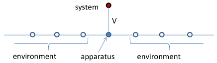
Figure 2: The origin of $\mathbb{Z}^{d}$ represents an apparatus which interacts with a system and environment.

Condition 4.

(No-interaction up to switching-on time) For $t\leq 0$ and an arbitrary state $\rho$ of the system, $(\rho\otimes\omega)\circ\alpha_{t}=(\rho\otimes\omega)\circ\alpha^{0}_{t}$ holds.

For $\tau>0$, let us consider the states $\Theta_{0}$ and $\Theta_{\tau}$ defined by $\Theta_{0}=\rho\otimes\omega$ and $\Theta_{\tau}=\rho\otimes(\omega\circ\beta_{-\tau})$. Due to Condition 4, the latter state can be rewritten as

$$\Theta_{\tau}=((\rho\circ\gamma_{\tau})\otimes\omega)\circ\alpha^{0}_{-\tau}=((\rho\circ\gamma_{\tau})\otimes\omega)\circ\alpha_{-\tau}.$$

We consider states at time $t=\tau$ for initial states $\Theta_{0}$ and $\Theta_{\tau}$. Although $\Theta_{0}\circ\alpha_{\tau}$ may become complicated, $\Theta_{\tau}\circ\alpha_{\tau}$ is written in a simple form as

$$\Theta_{\tau}\circ\alpha_{\tau}=(\rho\circ\gamma_{\tau})\otimes\omega.$$

Suppose that the dynamics $\alpha_{t}$ describes a measurement process for a PVM $\mathsf{P}=\{\mathsf{P}_{n}\}\subset\mathbf{B}(\mathcal{H})$ with its measurement time duration $\tau$. Let us take the Gelfand-Naimark-Segal (GNS) representation BR of the apparatus plus environment. That is, a state $\omega$ is represented by using a Hilbert space $\mathcal{K}$, a normalized vector $|\Omega\rangle\in\mathcal{K}$ and a representation $\pi$ as $\omega(A)=\langle\Omega|\pi_{\omega}(A)\Omega\rangle$. Let us consider the normalized vectors $|\phi_{n}\rangle\in\mathcal{H}$ satisfying $\mathsf{P}_{n}|\phi_{n}\rangle=|\phi_{n}\rangle$. Each $|\phi_{n}\rangle$ defines a state $\rho_{n}(B)=\langle\phi_{n}|B|\phi_{n}\rangle$ on the system for $B\in\mathbf{B}(\mathcal{H})$. As the dynamics describes a measurement process of $\mathsf{P}$, there exists a POVM $\mathsf{E}=\{\mathsf{E}_{n}\}\subset\mathbf{B}(\mathcal{H}_{0})\subset\mathfrak{A}$ such that

$$(\rho_{n}\otimes\omega)\circ\alpha_{\tau}(\mathbf{1}\otimes\mathsf{E}_{m})=\langle\phi_{n}\otimes\Omega|\pi(\alpha_{\tau}(\mathbf{1}\otimes\mathsf{E}_{m}))|\phi_{n}\otimes\Omega\rangle=\delta_{nm},$$

where $\pi=id\otimes\pi_{\omega}$ is a representation of the total observable algebra. Let us consider a pair of states $\{\rho_{+}=|+\rangle\langle+|,\rho_{-}=|-\rangle\langle-|\}$ on the system defined by $|\pm\rangle=\frac{1}{\sqrt{2}}(|\phi_{0}\rangle\pm|\phi_{1}\rangle)$. For any $\mathsf{A}\in\mathbf{B}(\mathcal{H})$, it holds that

$$|(\rho_{+}\otimes\omega-\rho_{-}\otimes\omega)\circ\alpha_{\tau}(\mathsf{A}\otimes\mathbf{1})| = 2|Im\langle\phi_{0}\otimes\Omega|\pi(\alpha_{\tau}(\mathsf{A}\otimes\mathbf{1}))|\phi_{1}\otimes\Omega\rangle|$$

$$\leq 2|\langle\phi_{0}\otimes\Omega|\pi(\alpha_{\tau}(\mathsf{A}\otimes\mathbf{1}))|\phi_{1}\otimes\Omega\rangle|$$

$$\leq 2\sum_{n}|\langle\phi_{0}\otimes\Omega|\pi(\alpha_{\tau}(\mathsf{A}\otimes\mathsf{E}_{n}))|\phi_{1}\otimes\Omega\rangle|$$

$$= 2\sum_{n}|\langle\phi_{0}\otimes\Omega|\pi(\alpha_{\tau}(\mathbf{1}\otimes\mathsf{E}^{1/2}_{n}))\pi(\alpha_{\tau}(\mathsf{A}\otimes\mathbf{1}))\pi(\alpha_{\tau}(\mathbf{1}\otimes\mathsf{E}^{1/2}_{n}))|\phi_{1}\otimes\Omega\rangle|$$

$$\leq 2\|\mathsf{A}\|\sum_{n}\langle\phi_{0}\otimes\Omega|\pi(\alpha_{\tau}(\mathbf{1}\otimes\mathsf{E}_{n}))|\phi_{0}\otimes\Omega\rangle^{1/2}\langle\phi_{1}\otimes\Omega|\pi(\alpha_{\tau}(\mathbf{1}\otimes\mathsf{E}_{n}))|\phi_{1}\otimes\Omega\rangle^{1/2}$$

$$= 2\|\mathsf{A}\|\sum_{n}\delta_{0n}\delta_{1n}=0.$$

Let $\rho_{\pm}(\tau)$ denote the restricted states of $(\rho_{\pm}\otimes\omega)\circ\alpha_{\tau}$ on the system. We can conclude that the pair of states $\rho_{+}(\tau)$ and $\rho_{-}(\tau)$ satisfies $\rho_{+}(\tau)=\rho_{-}(\tau)$. Therefore we can introduce $\rho(\tau)$ by $\rho(\tau)=\rho_{+}(\tau)=\rho_{-}(\tau)$.

We define a pair of states $|\pm^{\prime}\rangle\langle\pm^{\prime}|$ by $|\pm^{\prime}\rangle=e^{-\frac{H_{S}\tau}{\hbar}}|\pm\rangle$. The argument in the previous section is applied to derive $\min\{F(\rho(\tau),|+^{\prime}\rangle\langle+^{\prime}|),F(\rho(\tau),|-^{\prime}\rangle\langle-^{\prime}|)\}\leq\frac{1}{\sqrt{2}}$. Hereafter we assume $F(\rho(\tau),|+^{\prime}\rangle\langle+^{\prime}|)\leq\frac{1}{\sqrt{2}}$.

In the present case, since the environment is infinite, the energy fluctuation of the environment is usually infinite as well. Thus the direct application of our previous result gives only a trivial inequality. Considering the locality of the model, we can see that the region relevant to the dynamics of the system is finite, because the information propagates essentially at a finite speed. This finite information propagation speed $V_{\Phi}<\infty$ is given by the so-called Lieb-Robinson bound BR ; NS . This bound allows us to approximate the dynamics by that given by a “box Hamiltonian”. For an arbitrary $\epsilon>0$, and $v\geq V_{\Phi}$, there is a finite region $D$ such that for any $\mathsf{A}\in\mathbf{B}(\mathcal{H})$ and $t\in\mathbb{R}$,

$$\|\alpha_{t}(A)-\alpha_{t}^{\Lambda_{v|t|,D}}(A)\|\leq\epsilon\|\mathsf{A}\|,$$

where $\Lambda_{v|t|,D}:=\{x|\ ^{\exists}y\in D,d(x,y)<v|t|\}$ represents a “box”. Let us consider the approximated dynamics given by the box $\Lambda_{V_{\Phi}\tau,D}$. The states $\rho_{\pm}$ evolve into $\rho^{\prime}_{\pm}(\tau)$ in time $\tau$ following this approximated dynamics. For the box Hamiltonian $H_{\Lambda_{V_{\Phi}\tau,D}}$, we apply Theorem 2 to obtain

$$\cos\left(\frac{\Delta H_{\Lambda_{V_{\Phi}\tau,D}}}{\hbar}\tau\right)\leq F(\rho^{\prime}_{+}(\tau),|+^{\prime}\rangle\langle+^{\prime}|),$$

which is equivalent to

$$\frac{\Delta H_{\Lambda_{V_{\Phi}\tau,D}}}{\hbar}\tau\geq\mbox{Arccos}F(\rho^{\prime}_{+}(\tau),|+^{\prime}\rangle\langle+^{\prime}|).$$ (10)

To estimate how well the state $\rho^{\prime}_{+}(\tau)$ approximates the real state $\rho_{+}(\tau)$, we use a result obtained by Rastegin Rastegin .

Lemma 4.

For states $\rho_{0},\rho_{1},\sigma$, it holds that

$$\mbox{Arccos}F(\rho_{0},\rho_{1})\leq\mbox{Arccos}F(\rho_{0},\sigma)+\mbox{Arccos}F(\rho_{1},\sigma).$$

Applying this to (10), we obtain

$$\frac{\Delta H_{\Lambda_{V_{\Phi}\tau,D}}}{\hbar}\tau\geq\mbox{Arccos}F(\rho_{+}(\tau),|+\rangle\langle+|)-\mbox{Arccos}F(\rho_{+}(\tau),\rho^{\prime}_{+}(\tau)).$$

The last term on the right-hand side is bounded by the use of a relation between fidelity and trace distance, $1-F(\rho_{+}(\tau),\rho^{\prime}_{+}(\tau))\leq D(\rho_{+}(\tau),\rho^{\prime}_{+}(\tau)):=\sup_{\mathsf{A}:\|\mathsf{A}\|=1}|\mbox{tr}[(\rho_{+}(\tau)-\rho^{\prime}_{+}(\tau))\mathsf{A}]|$. Since it holds that

$$1-F(\rho_{+}(\tau),\rho^{\prime}_{+}(\tau))^{2}=(1-F(\rho_{+}(\tau),\rho^{\prime}_{+}(\tau)(1+F(\rho_{+}(\tau),\rho^{\prime}_{+}(\tau)))\leq 2D(\rho_{+}(\tau),\rho^{\prime}_{+}(\tau)),$$

we obtain

$$\mbox{Arccos}F(\rho_{+}(\tau),\rho^{\prime}_{+}(\tau))\leq\mbox{Arcsin}\sqrt{2D(\rho_{+}(\tau),\rho^{\prime}_{+}(\tau))}\leq\frac{\pi}{2}\sqrt{2D(\rho_{+}(\tau),\rho^{\prime}_{+}(\tau))}.$$

As $F(\rho_{+}(\tau),|+^{\prime}\rangle\langle+^{\prime}|)\leq\frac{1}{\sqrt{2}}$ holds, we conclude

$$\Delta H_{\Lambda_{V_{\Phi}\tau,D}}\cdot\tau\geq\frac{\pi\hbar}{4}-\frac{\pi\hbar}{2}\sqrt{2\epsilon},$$

which represents a starting point in the discussion of the spacetime uncertainty relation.

Let us give a rough sketch on the heuristic derivation of the spacetime uncertainty relation following FDR . For the relativistic dynamics, $V_{\Phi}$ in the above nonrelativistic model could be replaced by the speed of light $c$ and $D$ represents a relevant region of the local observable $\mathsf{A}$, and $\epsilon=0$. Thus we obtain for $\Gamma_{D}(\tau)=\{D+{\bf x}\in\mathbb{R}^{3}|{\bf x}^{2}\leq(c\tau)^{2}\}$,

$$\Delta H_{\Gamma_{D}(\tau)}\tau\geq\frac{\pi\hbar}{4}.$$

Assume that $D$ is a sphere with radius $R$. Then the volume of $\Gamma_{D}(\tau)$ is equal to $\frac{\pi}{3}(R+c\tau)^{3}$. Let us identify $\Delta H_{\Gamma_{D}(\tau)}$ with a mass $Mc^{2}$ in the region $\Gamma_{D}(\tau)$. The above inequality gives

$$Mc^{2}\tau\geq\frac{\pi\hbar}{4}.$$

For the mass to avoid the formation of a blackhole, $R+c\tau$ must exceed the Schwarzschild radius and

$$R+c\tau\geq\frac{2GM}{c^{2}}$$

holds. Thus we have the limitation,

$$\tau(R+c\tau)\frac{c^{4}}{2G}\geq\frac{\pi\hbar}{4}.$$

For small $\tau(\ll\frac{R}{c})$, this implies

$$\tau R\geq\frac{\pi\hbar G}{2c^{4}}.$$

VII Discussions

In this paper, we studied quantum measurements as physical processes. Each measurement is described as an interaction between a system and an apparatus. We investigated the energy fluctuation of the apparatus and the strength of interaction so that the system-plus-apparatus is regarded as a closed quantum system. We first examined the so-called standard model of measurement to find that this model needs an external system that switches on its measurement interaction. In this sense, the model is not closed. For the system-plus-apparatus to be genuinely closed, the quantum side must be made large enough to be capable of switching on the interaction autonomously. In this setting, we showed a trade-off relation between the measurement time duration and the energy fluctuation of the apparatus. This relation was obtained by combining two uncertainty relations; the information-disturbance relation and Mandelstam-Tamm uncertainty relation. We applied this relation to strengthen an argument regarding the spacetime uncertainty relation. In addition, we considered the strength of interaction between the system and the apparatus, and showed that there also exists a trade-off between the strength and the measurement time duration.

For an apparatus to evolve completely freely up to a certain time and then switch on a perturbation, the Hamiltonian must be two-sided unbounded. This unbounded nature is often unwelcome as it forces the apparatus to be an infinite or unstable system. To avoid this situation, we may weaken Condition 1 by allowing some error (see Example 2). This kind of weakening of the conditions has been often employed in studies on quantum clocks Peres ; BDM . A detailed study on more “physical” measurement models will be treated elsewhere.

A quantum apparatus in our problem can be understood as a device performing a specified task. This sort of device is studied in a context of programmable quantum gates HZbook ; Nielsen and the optimality of control has been recently discussed Bisio . It would be interesting to extend our result so as to be applicable to various tasks other than measurement. For instance the famous Einstein photon box BuschTEUR ; Busch1 could, we hope, be revisited.

While our treatment of spacetime uncertainty relations agrees with physical intuition, there remain things to be improved. The discrete space is the most crucial drawback in our model. We should treat the spacetime as a continuum, or as a flat Minkowski spacetime as the first natural setting. In order to achieve this, the time translation group $\mathbb{R}$ should be generalized to the Poincaré group $\mathcal{P}_{+}^{\uparrow}$. Then the localization of event will be made much clearer and a covariant spacetime uncertainty relation is expected to be obtained. Such an extension and refinement of our analysis to $\mathcal{P}_{+}^{\uparrow}$ (or general Lie group $G$) is an important problem which we hope will be studied elsewhere.

As a final remark, we want to point out that an external classical clock is assumed in our study. If we shift the interface so that the quantum side contains a clock, the time is not anymore an extrinsic parameter but instead will become a relative quantity depending on the quantum clock PageWootters ; Milburn ; Giovannetti . A related concept, the notion of reference frame, has been recently studied extensively BRS ; mlbshort ; VSP .
Acknowledgements I am grateful to anonymous referees for valuable comments, and to Leon Loveridge for many helpful remarks. This work was supported by KAKENHI Grant Number 15K04998.

Appendix A Proof of Theorem 4

Proof.

For simplicity, we assume that $t_{0}=0$ and that $\sigma(0)(=|\phi(0)\rangle\langle\phi(0))|$ is pure. Let us consider two states $\Theta_{0}(0)$ and $\Theta_{t}(0)$ $(0\leq t\leq\frac{\pi\hbar}{2\Delta H_{c}})$ defined by

$$\Theta_{0}(0) := \rho(0)\otimes|\phi(0)\rangle\langle\phi(0)|$$

$$\Gamma_{t}(0) := \rho(0)\otimes|\phi(-t)\rangle\langle\phi(-t)|.$$

These states evolve with the Hamiltonian $H=H_{S}+H_{A}+V$. Let us denote the states at time $t$ by $\Theta_{0}(t)$ and $\Gamma_{t}(t)$. While $\Theta_{0}(t)$ may have a complicated form, $\Gamma_{t}(t)$ has a simple form,

$$\Gamma_{t}(t)=\rho^{0}(t)\otimes|\phi(0)\rangle\langle\phi(0)|,$$

where we used Lemma 2. Because the fidelity between two states is invariant under unitary evolution Nielsen , it follows that

$$F(\Theta_{0}(0),\Gamma_{t}(0))=F(\Theta_{0}(t),\Gamma_{t}(t)).$$

The left-hand side of the above equation becomes

$$F(\Theta_{0}(0),\Gamma_{t}(0))=|\langle\phi(0)|\phi(-t)\rangle|$$

and the right-hand side is bounded as

$$F(\Theta_{0}(t),\Gamma_{t}(t))\leq F(\rho(t),\rho^{0}(t)),$$

where we utilized the fact that the fidelity decreases for restricted states Nielsen . Thus it holds that

$$|\langle\phi(0)|\phi(-t)\rangle|\leq F(\rho(t),\rho^{0}(t)).$$

The left-hand side of this inequality represents the speed of time evolution of the apparatus and is bounded. Let us fix a value $0\leq F_{0}\leq 1$ and denote by $\tau_{F}$ the minimum time $t$ attaining $F(\rho(t),\rho^{0}(t))\leq F_{0}$. Then we obtain,

$$\tau_{F_{0}}\cdot\Delta_{\alpha}(H)\geq 2\hbar\arccos\frac{F_{0}+1-\alpha}{\alpha}.$$

For this process to describe a measurement process, there must be an initial state attaining $F(\rho(t),\rho^{(}0))\leq\frac{1}{\sqrt{2}}$. Thus we obtain

$$\tau\cdot\Delta_{\alpha}(H)\geq 2\hbar\arccos\frac{\frac{1}{\sqrt{2}}+1-\alpha}{\alpha}.$$

∎

Corollary 2.

For $\alpha=\frac{1}{2}\left(\frac{1}{\sqrt{2}}+1\right)$, it holds that

$$\tau\cdot\Delta_{\alpha}(H)\geq\frac{2\pi\hbar}{3}.$$

Appendix B Proof of Theorem 5

Proof.

We mimic the proof of Theorem 3. We consider the dynamics from time $t=t_{0}$ to $t=t_{0}+\tau$. Suppose that $0$ and $1$ are possible outcomes. We consider two states $|0\rangle$ and $|1\rangle$ satisfying $P_{0}|0\rangle=|0\rangle$, $P_{1}|0\rangle=0$, $P_{1}|1\rangle=|1\rangle$, and $P_{0}|1\rangle=0$ and define $|\pm\rangle:=\frac{1}{\sqrt{2}}(|0\rangle+|1\rangle)$. We consider a pair of initial states $|\pm\rangle\langle\pm|\otimes\sigma(t_{0})$. The states to be compared are $\rho_{\pm}:=\mbox{tr}_{\mathcal{K}}[e^{-i\frac{H}{\hbar}\tau}(|\pm\rangle\langle\pm|\otimes\sigma(t_{0}))e^{i\frac{H}{\hbar}\tau}]$. For an arbitrary operator $\mathsf{A}$ on the system, it holds that

$$|\mbox{tr}[e^{-i\frac{H}{\hbar}\tau}(|(+\rangle\langle+|-|-\rangle\langle-|)\otimes\sigma(t_{0}))e^{i\frac{H}{\hbar}\tau}(\mathsf{A}\otimes\mathbf{1})]$$

$$\leq 2\|\mathsf{A}\|\sum_{n}\langle 0\otimes\phi(t_{0})|e^{i\frac{H}{\hbar}\tau}(\mathbf{1}\otimes\mathsf{E}_{n})e^{-i\frac{H}{\hbar}\tau}|0\otimes\phi(t_{0})\rangle^{1/2}\langle 1\otimes\phi(t_{0})|e^{i\frac{H}{\hbar}\tau}(\mathbf{1}\otimes\mathsf{E}_{n})e^{-i\frac{H}{\hbar}\tau}|1\otimes\phi(t_{0})\rangle^{1/2}$$

$$= 2\|\mathsf{A}\|\sum_{n}P(n||0\rangle\langle 0|)^{1/2}P(n||1\rangle\langle 1|)^{1/2}$$

$$= 2\|\mathsf{A}\|\left(P(0||0\rangle\langle 0|)^{1/2}P(0||1\rangle\langle 1|)^{1/2}+P(1||0\rangle\langle 0|)^{1/2}P(1||1\rangle\langle 1|)^{1/2}+\sum_{n\neq 0,1}P(n||0\rangle\langle 0|)^{1/2}P(n||1\rangle\langle 1|)^{1/2}\right)$$

$$\leq 2\|\mathsf{A}\|\left(P(0||1\rangle\langle 1|)^{1/2}+P(1||0\rangle\langle 0|)^{1/2}+(\sum_{n\neq 0,1}P(n||0\rangle\langle 0|))^{1/2}(\sum_{n\neq 0,1}P(n||1\rangle\langle 1|))^{1/2}\right)$$

$$\leq 6\|A\|\sqrt{P_{error}}.$$

Thus we obtain $D(\rho_{+},\rho_{-}):=\sup_{\mathsf{A}:\|\mathsf{A}\|=1}|\mbox{tr}[(\rho_{+}-\rho_{-})\mathsf{A}]|\leq 6\sqrt{P_{error}}$. To estimate the magnitude of this perturbation we consider unitary evolution governed by the Hamiltonian $H_{S}$. In time $\tau$, this “unperturbed” dynamics changes $|\pm\rangle$ to a pair of orthogonal states $|\pm^{\prime}\rangle$ of the system. We then estimate $F(\rho_{+},|+^{\prime}\rangle\langle+^{\prime}|)$ and $F(\rho_{-},|-^{\prime}\rangle\langle-^{\prime}|)$. As $|\pm^{\prime}\rangle$ are orthogonal, we have

$$F(\rho_{+},|+^{\prime}\rangle\langle+^{\prime}|)^{2}+F(\rho_{-},|-^{\prime}\rangle\langle-^{\prime}|)^{2} = \langle+^{\prime}|\rho_{+}|+^{\prime}\rangle+\langle-^{\prime}|\rho_{-}|-^{\prime}\rangle$$

$$= \langle+^{\prime}|\rho_{+}|+^{\prime}\rangle+\langle-^{\prime}|\rho_{+}|-^{\prime}\rangle+\langle-^{\prime}|\rho_{-}-\rho_{+}|-^{\prime}\rangle$$

$$\leq \mbox{tr}[\rho_{+}]+D(\rho_{+},\rho_{-})$$

$$\leq 1+6\sqrt{P_{error}}.$$

Thus we can conclude

$$\min\{F(\rho,|+^{\prime}\rangle\langle+^{\prime}|),F(\rho,|-^{\prime}\rangle\langle-^{\prime}|)\}\leq\sqrt{\frac{1+6\sqrt{P_{error}}}{2}}.$$

We assume $F(\rho,|+^{\prime}\rangle\langle+^{\prime}|)\leq\sqrt{\frac{1+6\sqrt{P_{error}}}{2}}$. Combining it with Theorem 2 by putting $\rho(t_{0})=|+\rangle\langle+|$, we obtain

$$\cos\left(\frac{\tau\Delta H_{A}}{\hbar}\right)\leq\sqrt{\frac{1+6\sqrt{P_{error}}}{2}}.$$

This ends the proof. ∎

References

- (1) J. A. Wheeler and W. Zurek, Quantum Theory and Measurement, Princeton University Press, 1984.
- (2) J. von Neumann, Mathematical Foundations of Quantum Mechanics , Princeton University Press, 1955.
- (3) P. Busch, P. Lahti and P. Mittelstaedt, The Quantum Theory of Measurement, Springer, 1996.
- (4) P. Busch, M. Grabowski and P. Lahti, Operational Quantum Physics, Springer, 1995.
- (5) T. Heinosaari and M. Ziman, The Mathematical Language of Quantum Theory, Cambridge University Press, 2012.
- (6) J. S. Bell, Speakable and Unspeakable in Quantum Mechanics, Cambridge University Press 2004.
- (7) While a measurement process consists of the “information transfer” described by the time evolution of a composite system and the state reduction conditional to each measurement outcome, we treat only the former. See Ozawareduction for the relevant discussions.
- (8) M. Ozawa, Fortschr. Phys. 46, 615 (1998).
- (9) M. Ozawa, J. Math. Phys. 25, 79 (1984).
- (10) Y. Aharonov and D. Bohm, Phys. Rev. 122, 1649 (1961).
- (11) P. Busch, Found. Phys. 20, 33 (1990).
- (12) P. Busch, in Time in Quantum Mechanics, eds. J. G. Muga, R. Sala Mayato, I.L. Egusquiza, Springer-Verlag, Berlin 2nd ed. (2008).
- (13) For a given total Hamiltonian there is an ambiguity in dividing it into three parts as . In this paper, by imposing conditions which are explained later, this arbitrariness is reduced to some extent. Although there remains arbitrariness even with these conditions, our results do not depend on the choice of the division.
- (14) G. C. Hegerfeldt, Phys. Rev. Lett. 72 596 (1994).
- (15) L. Ahlfors, Complex Analysis, McGraw-Hill, 1979.
- (16) R. Haag, Local Quantum Physics, Springer, 1992.
- (17) M. Nielsen and I. Chuang, Quantum Computation and Quantum Information, Cambridge University Press, (2000).
- (18) L. Mandelstam and I. G. Tamm, J. Phys. U.S.S.R. 9, 249 (1945).
- (19) P. Busch, Found. Phys. 20, 1 (1990).
- (20) P. Pfeifer, Phys. Rev. Lett. 70, 3365 (1993).
- (21) B. Janssens and H. Maassen, J. Phys. A: Math. Gen. 39, 9845 (2006).
- (22) J. Uffink, Am. J. Phys. 61, 935 (1993).
- (23) T. Miyadera and H. Imai, Phys. Rev. A 78, 052119 (2008).
- (24) T. Miyadera, J. Math. Phys. 52, 072105 (2011).
- (25) T. Heinosaari and T. Miyadera, Phys. Rev. A 88, 042117 (2013).
- (26) T. Miyadera, Phys. Rev. A 83, 052119 (2011).
- (27) C. A. Mead, Phys. Rev. 135, B849 (1964).
- (28) T. Yoneya, Prog. Theor. Phys. 103, 1081 (2000).
- (29) S. Doplicher, K. Fredenhagen and J. E. Roberts, Commun. Math. Phys. 172, 187 (1995).
- (30) O. Bratteli and D. Robinson, Operator Algebras and Quantum Statistical Mechanics 1 & 2, Springer, 1997.
- (31) B. Nachtergaele and R. Sims, New Trends in Mathematical Physics, 591 (2009).
- (32) A. E. Rastegin, Phys. Rev. A 67, 012305 (2003).
- (33) A. Peres, Am. J. Phys. 42, 552 (1980).
- (34) V. Buzek, R. Derka and S. Massar, Phys. Rev. .Lett.. 82, 2207 (1999).
- (35) A. Bisio, G. Chiribella, G. M. D’ariano, S. Facchini and P. Perinotti, Phys. Rev. A 81, 032324 (2010).
- (36) D. N. Page and W. K. Wootters, Phys. Rev. D 27, 2885 (1983).
- (37) G. J. Milburn and D. Poulin, Int. J. Quantum Inform., 04, 151 (2006).
- (38) V. Giovannetti, S. Lloyd and L. Maccone, Phys. Rev. D 92, 045033 (2015).
- (39) S. D. Bartlett, T. Rudolph and R. W. Spekkens, Rev. Mod. Phys. 79, 555 (2007).
- (40) T. Miyadera, L. Loveridge and P. Busch, J. Phys. A: Math. Theor. 49, 185301 (2016).
- (41) L. Loveridge, P. Busch and T. Miyadera, arXiv: 1604.02836.