Experimental quantum tomography of a homodyne detector

Abstract

We suggest and demonstrate a tomographic method to fully characterize homodyne detectors at the quantum level. The operator measure associated with the detector is expanded in the quadrature basis and probed with a set of coherent states. The coefficients of the expansion are retrieved using a least squares algorithm. We then validate the reconstructed operator measure on nonclassical states. Finally, we exploit results to estimate the overall quantum efficiency of the detector.

I Introduction

Balanced homodyne detection is a crucial detection technique for continuous variable quantum technology and lies at the core of many quantum optics experiments Lvovsky and Raymer (2009); Mauro D’Ariano et al. (2003); Welsch et al. (1999). From its first proposal for the measurement of quadrature squeezing, to its current extensive use in the fields of quantum tomography, quantum communication and quantum metrology Vogel and Risken (1989); Smithey et al. (1993); D’Ariano et al. (1994); Armen et al. (2002); D’Auria et al. (2009); Wittmann et al. (2010); Chi et al. (2011); Blandino et al. (2012); Kumar et al. (2012); Olivares et al. (2013); Berni et al. (2015); Cialdi et al. (2016), this detection scheme has carved its place into experimental quantum optics. Besides quantum optical systems, homodyne detection extends its reach to the whole field of continuous variable quantum technologies, spanning from atomic systems Gunawardena and Elliott (2007); Gross et al. (2011) to quantum optomechanics Verhagen et al. (2012).

Advances in technology promoted the spread of many different configurations of this versatile apparatus, tailored to disparate experimental needs. Such a wide range of applications calls for reliable ways to fully characterize homodyne detectors. Each specific setup relies on classical calibrations in order to gain the most general description of the apparatus and of the relationship between the input state and the measurement output. Recently, a characterisation of homodyne detection, only used as a phase-insensitive photon counter, was demonstrated Cooper et al. (2014). However, a general and reliable model for the description of the fully phase-sensitive homodyne detection in the form of a Quantum Detector Tomography (QDT) is, in fact, still lacking.

The pioneering proposals for QDT Luis and Sánchez-Soto (1999); Fiurášek (2001); D’Ariano et al. (2004a); D’Ariano and Perinotti (2007) were followed by the experimental characterization of an avalanche photodiode, in both single and time-multiplexed configurations, for the detection of up to eight photons Lundeen et al. (2009). Subsequent works developed the idea, including the effect of decoherence onto the operator description D’Auria et al. (2011), or different detection devices, such as superconducting nanowires Akhlaghi et al. (2011) and TES based systems Brida et al. (2012a, b). However, these are detectors devoted to photon counting, whose description is entirely embedded in the diagonal sector of the Fock space. Only recently, a specific phase-sensitive hybrid scheme, in the form of a weak homodyne detector based on photon counting, was the object of an experimentally realized QDT Zhang et al. (2012). In this paper, we move several crucial steps forward, and present a theoretical and experimental realization of QDT for homodyne detector, i.e. the most commonly used form of a fully phase-sensitive detector, whose operators are naturally described in phase space.

The quantum description of any detector is given by a positive operator-valued measure (POVM), i.e. a set of positive operators $\left\{\Pi_{n}\right\}$, giving a resolution of identity $\sum_{n}\Pi_{n}={\mathbb{I}}$. The determination of these operators is, in turn, the main goal of detector tomography. Given an input state $\rho$, the Born rule states that $p_{n}^{\rho}=\mathtt{Tr}\!\left[\rho\,\Pi_{n}\right]$ is the probability of obtaining the outcome $n$ when the generalized observable described by $\Pi$ is being measured. The inversion of this formula allows the reconstruction of the operators $\Pi_{n}$ from the experimentally sampled probability distribution $p_{n}^{\rho}$, over a suitable set of known states $\rho$. These must form a tomographically complete set, spanning the Hilbert subspace where the POVM elements are defined on D’Ariano et al. (2000).

The simplest choice for a continuous variable system is a set of coherent states. They provide an overcomplete basis for the Fock space, and it has already been proved that even 1-dimensional discrete collections of coherent states form a complete basis, and may be used to reconstruct classical and non-classical states Janszky and Vinogradov (1990); Janszky et al. (1995). In fact, the experimental distributions of the outcomes for a set of coherent states already provide a full representation of the detector operators, in the form of a sample of their Q-functions

$$Q_{n}(\alpha)=\frac{1}{\pi}\left\langle\alpha\right|\Pi_{n}\left|\alpha\right\rangle=\frac{1}{\pi}\mathcal{P}_{n}^{\alpha}\,,$$

where $\{{\mathcal{P}^{\alpha}_{n}}\}$ represents the probability distribution for a coherent state. However, this representation is not suitable to provide a complete and reliable characterization of the detector. In fact, any subsequent use of this reconstruction scheme to predict the outcome of the measurement for a different signal would involve the (numerical) evaluation of the trace rule in the phase-space as

$$\mathtt{Tr}\!\left[\rho\,\Pi_{n}\right]=\int_{\mathbb{C}}\!d^{2}\alpha\,P[\rho](\alpha)\,Q_{n}(\alpha)\,,$$

where the Glauber P-function $P[\rho](\alpha)$ is singular for any nonclassical state, and thus not suitable for sampling. In order to overcome this problem we suggest an expansion in the quadrature basis of the operator measure associated with the detector, using as probe a set of coherent states. We then obtain the coefficients of the expansion using a least squares algorithm on a sufficiently large sample of data. We also validate the experimentally obtained POVM by reconstructing nonclassical known states. Finally, we exploit results to estimate the overall quantum efficiency of the detector.

The paper is structured as follows. In Section II we review the description of homodyne detection and introduce the algorithm employed for the reconstruction of its POVM. In Section III we describe our experimental apparatus, whereas in Section IV we present results of the reconstruction, as well as their validation on nonclassical states. Section V closes the paper with some concluding remarks.

II Homodyne Detection

A homodyne detector is a fully phase sensitive apparatus that provides a complete characterization of any given state of a single-mode radiation field Leonhardt (1997). This state, the signal, is sent to a balanced beam splitter, where it interferes with an intense coherent field, the local oscillator, usually coming from the same laser source. The phase of the signal has then a precise value $\phi$ with respect to the local oscillator, and can be adjusted by means of a piezo-actuated mirror. The two outputs of the beam splitter are then focused on two photodiodes, and the resulting photocurrents subtracted and analyzed. It can be shown that, in the approximation of high amplitude $\left|\beta\right|$ of the local oscillator, the measurement associated to this detector corresponds to

$${X}=\frac{{a}{b}^{\dagger}+{a}^{\dagger}{b}}{\sqrt{2}\left|\beta\right|}\underset{\left|\beta\right|\gg 1}{\longrightarrow}\frac{{a}^{\dagger}e^{\imath\phi}+{a}\,e^{-\imath\phi}}{2}={x}_{\phi}$$ (1)

where ${a}$ and ${b}$ are the mode operators for the signal and the local oscillator, respectively. The operator ${b}$ was replaced by $\left|\beta\right|e^{\imath\phi}$ in Eq. (1) by considering its action onto the local oscillator, that can be treated as a coherent state $\left|\beta\right\rangle$. The operation connected to the working scheme of this detector is therefore the measurement of the quadrature operator ${x}_{\phi}$ on the signal mode. Such a link states the equivalence between the discrete spectrum of the operator ${X}$ and the continuous one of the quadrature, due to the high intensity of the local oscillator, that can be consequently treated classically. This equivalence can be extended to the characteristic functions

$$\mathtt{Tr}\!_{a,b}\!\left[e^{\imath\lambda{X}}\rho\otimes\left|\beta\right\rangle\!\left\langle\beta\right|\right]\underset{\left|\beta\right|\gg 1}{\longrightarrow}\mathtt{Tr}\!_{a}\!\left[e^{\imath\lambda{x}_{\phi}}\rho\right]$$ (2)

assuring the equivalence of all moments D’Ariano et al. (2004b).

The key feature of homodyne detection is its ability to discern between different phase values of an input signal, setting itself apart from the photon counting detectors that have been characterized in the past. A straightforward choice for a basis in which representing the POVM elements of a phase insensitive device is the number basis, in the form $\Pi_{k}=\sum_{n=0}^{+\infty}\pi_{n}^{(k)}\left|n\right\rangle\!\left\langle n\right|$, where $\left|n\right\rangle\!\left\langle n\right|$ is the projector onto the n-photon Fock state. Such a description is no longer suitable for our apparatus, that hinges on a phase-sensitive operation scheme. Off-diagonal elements in the number-basis expansion could enclose phase-sensitive properties, as was done in Zhang et al. (2012), but reconstruction of the detector operators would become increasingly difficult due to the high dimension of the Hilbert space the POVM would be defined in.

II.1 The reconstruction algorithm

A suitable basis to expand the POVM $\Pi(x)$ of a phase-sensitive detector for continuous variable systems is the set $\left\{\left|y\right\rangle\!\left\langle y\right|\right\}_{y\in\mathbb{R}}$ of eigenstates of a quadrature operator ${x}_{\phi}$, e.g. setting $\phi=0$

$$\Pi(x)=\int\!dy\,g^{(x)}_{y}\left|y\right\rangle\!\left\langle y\right|\,.$$ (3)

The detector has now a Q-function representation given by

$$\mathcal{P}_{\alpha}(x) =\left\langle\alpha\right|\Pi(x)\left|\alpha\right\rangle$$

$$=\int\!\!dy\,g^{(x)}_{y}\sqrt{\frac{2}{\pi}}\,\exp\left\{-2(y-\left|\alpha\right|)^{2}\right\}\,,$$ (4)

where the matrix $g^{(x)}_{k}$ contains all the information needed to describe the response of the detector. The set of operators $\left\{\Pi(x)\right\}$ can then be discretized, reflecting the experimental sampling during the measurement process, and be confined to a selected portion of the quadrature range, say $\left[x_{\min},\,x_{\max}\right]$. The expansion on the quadrature basis $\left\{\left|y\right\rangle\!\left\langle y\right|\right\}$ can be discretized as well, reducing the number of POVM elements. Equation (II.1) may be rewritten as

$$\Pi_{j}\equiv\Pi(x_{j})=\sum_{k}g^{j}_{k}\left|y_{k}\right\rangle\!\left\langle y_{k}\right|\,.$$ (5)

The analogue of Eq. (II.1), i.e. ${\mathcal{P}}_{\alpha}(x_{j})=\langle\alpha|\Pi(x_{j})|\alpha\rangle$, can now be compared to experimental results and may be inverted to find the matrix $\mathbf{g}$. To this purpose, starting from a set of coherent states with calibrated amplitudes $\left\{\left|\tilde{\alpha}_{s}\right|\right\}$, we use a least-squares method:

$$g^{j}_{k}=\underset{\left\{g_{k}^{j}\right\}>0}{\mathtt{arg\,\,min}}\left\{\sum_{j}\sum_{s}\left[p_{\tilde{\alpha}_{s}}(x_{j})-\mathcal{P}_{\tilde{\alpha}_{s}}(x_{j})\right]^{2}\right\}\,,$$ (6)

where $p_{\tilde{\alpha}_{s}}(x_{j})$ is the experimentally observed distribution for the coherent state with amplitude $\left|\tilde{\alpha}_{s}\right|$. A pictorial representation of the algorithm is presented in Fig. 1(a). The algorithm retrieves the matrix $\mathbf{g}$ by comparing the experimentally sampled distributions to the corresponding Q - function representation. Starting from a coherent state of amplitude $\left|\tilde{\alpha}_{s}\right|$ and a quadrature value $x_{j}$, the algorithm finds the set of coefficients $g^{j}_{k}$ that minimises the difference between $p_{\tilde{\alpha}_{s}}(x_{j})$ and $\mathcal{P}_{\tilde{\alpha}_{s}}(x_{j})$. Experimental imperfections and fluctuations, corresponding to the shaded blue area in Fig. 1(a), degrade this relationship and “switch on” new coefficients in the expansion of Eq. (II.1). At the same time, each calibrated amplitude $\left|\tilde{\alpha}_{s}\right|$ is associated to a rescaled value $\left|\alpha_{s}\right|=\left|\tilde{\alpha}_{s}\right|\gamma_{s}$, to explicitly include the detector finite efficiency. The least squares algorithm of Eq. (6) performs this minimisation simultaneously for all the quadrature values $x_{j}\in\left[x_{\min},\,x_{\max}\right]$ and all the coherent states in the set. The detector response is then fully contained in the matrix $\mathbf{g}$.

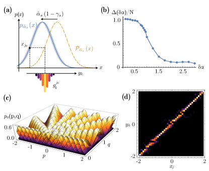
Figure 1: (Color online) Quantum tomography of a homodyne detector. A pictorial representation of the least-squares algorithm is reported in panel (a). The experimentally sampled probability distributions $p_{\tilde{\alpha}}(x)$ (solid blue) are compared to the Q - function representation $\mathcal{P}_{\tilde{\alpha}}(x)$ (dashed yellow). This is shown dashed to visualise the discretisation of Eq. (3). Panel (b) shows the efficiency of reconstruction as a function of increasing amplitude spacing in the tomographic set. The function $\Delta(\delta\alpha)$ is here normalized to the matrix dimension $N$. A sharp transition can be seen as the spacing between the states of the set approaches the maximum for the overlap function of Eq. (8). Panel (c) shows the phase space representation of the full set of coherent states used for tomography. Panel (d) shows the result of the reconstruction obtained imposing $\left|\alpha_{s}\right|=\left|\tilde{\alpha}_{s}\right|$. Notice the (expected) diagonal shape.

If we look back at Eq. (3), it is quite natural to link the characteristics of the matrix ${\mathbf{g}}$ to the features of the detector reconstruction. Each matrix row $g^{j}_{k}$ associates a quadrature value $x_{j}$ to a set of projectors on quadrature eigenstates, with weights given by the coefficients in Eq. (5). For an ideal detector, the matrix is diagonal $g^{j}_{k}=\delta_{kj}$, i.e. the only nonzero coefficient associates a quadrature value $x_{j}$ to its projector $\left|x_{j}\right\rangle\!\left\langle x_{j}\right|$. As we have seen, experimental imperfections will degrade this one-to-one relationship, spreading the coefficients around a central value. At the same time, the full array of coefficients $\gamma_{s}$ provides a unified model for the response of the detector. A detector tomography devised in this way is general enough for application to different configurations of the homodyne detection.

Let us now focus on the tomographic set, and in particular on the characteristics required to perform a reliable reconstruction. To this aim we have performed simulated experiments with sets having an increasing number of equidistant coherent states, with amplitudes in a given range $\alpha\in[-3,\,3]$, and measured at the same phase $\phi=0$. For each set the matrix representation of the detector $g^{j}_{k}$ was retrieved, and associated to the amplitude spacing $\delta\alpha$ between the coherent states in the set. Since the identity matrix ${\mathbb{I}}$ is the ideal-case solution of the reconstruction algorithm, we consider the following function of the amplitude spacing $\delta\alpha$

$$\Delta(\delta\alpha)=\mathtt{Tr}\!\left[\mathbb{I}\cdot\left[g^{j}_{k}\right]_{{\delta\alpha}}\right]$$ (7)

as a figure of merit to assess tomographic sets, e.g. to find the minimal $\delta\alpha$ corresponding to a reliable reconstruction.

For a perfect reconstruction, the two matrices are both the identity and $\Delta$ reduces to the dimension of the matrix $\mathbf{g}$. In the opposite case, more and more elements on the diagonal will be voided, and the trace will decrease. In Fig. 1(b) we show the results: a steep transition, corresponding to a deterioration of the reconstruction, appears for $\delta\alpha\simeq 0.7$. A similar conclusion may be obtained theoretically upon considering the overlap of two Gaussian $p_{\sigma}(x,x_{0})$ of equal standard deviation $\sigma$ but varying center $x_{0}$, i.e.

$$f(y)=\sqrt{\pi}\int_{-\infty}^{+\infty}\!\!\!\!\!\!\!dx\,p_{\sigma}(x,x_{0})\,p_{\sigma}(x,x_{0}+y)\,.$$ (8)

In particular, the function $y\cdot f(y)$ may be used to assess the tomographic set of coherent states, as it captures, roughly speaking, the trade-off between an increasing spacing and a decreasing overlap. Upon substituting $\sigma=0.5$, as it is for coherent states, we have that $y\cdot f\left(y\right)$ has a maximum at $y_{\max}=2^{-1/2}\simeq 0.707$, in good agreement with the value obtained by simulated experiments via Eq. (7). The reliability of this estimation has been then confirmed experimentally (see below).

III Experimental apparatus

A schematic diagram of the experimental setup is shown in Fig. 2. The apparatus is based on a mode-locked Ti:sapphire laser (Spectra-Physics Tsunami) providing, after suitable splitting, both the local oscillator (LO) beam for balanced homodyne detection and the probe coherent states for detector tomography. The laser emits $2$ ps pulses at a central wavelength of $78$5 nm, with a repetition rate of $82$ MHz. The detector characterized in this paper is an optical homodyne apparatus, operating in the time domain at high sampling frequency Zavatta et al. (2002, 2006). Amplitudes of the probe coherent states were selected by means of a reflective-coating glass attenuator. Precise calibration of each state is done by means of a Type I BBO crystal cut for degenerate spontaneous down-conversion (SPDC), pumped by the frequency doubled portion of the main laser beam. The injection of the probe coherent states into the signal path of the SPDC triggers the stimulated emission of downconverted photon pairs in the same mode (thus generating single-photon-added coherent states, SPACSs Zavatta et al. (2004a)) and in the idler mode, at a rate proportional to $1+\left|\alpha\right|^{2}$, where $\alpha$ is the amplitude of the incoming coherent state. Such a procedure provides a precise standard-free calibration of the input amplitude Migdall (1999) by means of the ratio between the count rate of stimulated and spontaneous events pursuing the idea of a calibration-free characterization.

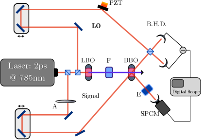
Figure 2: (Color online) Schematic diagram of the experimental setup. Picosecond-duration pulses at 785 nm are split by two high-transmission beam splitters. A first beam serves as the local oscillator (LO) for balanced homodyne detection (B.H.D.), while a second provides the probe coherent states for detector tomography. Optical delay lines provide synchronization, while the probe amplitude is adjusted with the attenuator (A). The main portion of the beam is frequency doubled in a LBO crystal, and then spatially and spectrally filtered by means of a pin-hole and a Michelson interferometer (F). It finally serves as the pump for a type-I BBO crystal for parametric down conversion, whose idler mode is used for calibration means and, after narrow Etalon spectral filtering (E), as a trigger signal.

IV Detector Tomography

In our detector tomography we have focused attention to the range $x\in\left[-2,\,2\right]$ probed by a tomographic set of coherent states with amplitudes $\alpha_{s}\in\{-3,\,3\}$. Our set is made of coherent states with $12$ different amplitudes, each one measured at $9$ different phase values between 0 and $\pi$. The full set is represented in Fig. 1(c).

As a first step we have performed a preliminary validating step of our reconstructing algorithm, by neglecting the rescaling factors $\gamma_{s}$. The set of amplitudes $\left\{\alpha_{s}\right\}$ has been measured with the homodyne detector, as the mean value of the probability distributions, and the coefficient matrix $\mathbf{g}$ has been retrieved imposing $\left|\tilde{\alpha}_{s}\right|=\left|\alpha_{s}\right|$. The result, reported in Fig. 1(d), presents the expected diagonal shape, partially blurred by fluctuations. The homodyne detection model obtained in this way may efficiently describe the detector behavior on several classical and non classical states.

Upon confirmation of the effectiveness of our method, we selected a reduced collection of coherent states, concentrating on those with a null or $\pi$ phase difference between the signal and the local oscillator. This set of $25$ coherent states has been then inserted into the algorithm of Eq. (6) together with the set of calibrated amplitudes $\left\{\tilde{\alpha}_{s}\right\}$, and the results are shown in Fig. 3(a). The retrieved matrix showed the expected diagonal shape, with an experimental spread around the central value. The array of coefficients $\gamma_{s}$ is reported in Fig. 3(b). An estimate for the uncertainty is obtained from the inverse of the second derivative of the function minimized in the least-squares algorithm. This uncertainty is increasing for decreasing values of $\alpha$, since for the limiting case of $\alpha=0$ our model is not defined. It was then used to weight the $\gamma_{s}$, and get a final mean value of $\bar{\gamma}_{0}=0.90\pm 0.03$.

Figure 3: (Color online) Quantum tomography of a homodyne detector. Panel (a) shows the matrix $g_{k}^{j}$ representing the expansion of the POVM elements in the quadrature basis. By comparison of this matrix with that of Fig. 1(d) one notices the spread of the coefficients around the diagonal, due to the additional parameters $\gamma_{s}$. These are reported in blue in the plot of Fig. 3(b), where the shaded area represents an estimate of the uncertainty, obtained through the second derivative of the function in Eq. (6). In a similar fashion, the mean value $\bar{\gamma}_{0}$ and its uncertainty are indicated in solid and shaded yellow. These results were then validated on the reconstruction of nonclassical states. In panels (c) and (d) we report the experimentally reconstructed Wigner functions for the Fock state $|1\rangle$ and for a single photon-added coherent state. The side plots in both panels show the Wigner marginal distributions (yellow), which are both very close to their representations in the detector description (the uncertainty due to the spread of $\bar{\gamma}_{0}$ is given by the blue-shadowed areas).

IV.1 POVM validation

The aim of quantum detector tomography is to fully characterize a given detector by retrieving the set of operators that fully describes its measurement process. In order to validate our technique for QDT, we have employed the reconstructed POVM to reproduce measurements performed on known states. In particular, we have tested the POVM on two kinds of nonclassical states: a single-photon Fock state and a SPACS with $\alpha=0.5$. These two states have been first measured in our setup, and the experimental results have been then compared to those obtained for the same states using the reconstructed detector POVM. The photon addition scheme of our setup, fundamental for the generation of these two states, had been previously characterised Zavatta et al. (2004b), and the operator ${a}^{\dagger}$ had been found to apply to a given input state with preparation efficiency $\zeta\approx 0.91$. The measured quadrature distributions for the Fock state and the SPACS, reported in Fig. 3(c) and 3(d), are in excellent agreement with the expected Q-function representation based on the tomography of our homodyne detector. The robustness and reliability of our method has been thus confirmed and we proved that the specific experimental realization of the detector, which depends on several parameters (like the detrector quantum efficiency, the degree of mode matching, the alignment, etc.), can be efficiently captured by the tomographic procedure. We also proved that the results of subsequent measurements can be effectively reproduced.

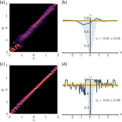
Figure 4: (Color online) Changing the number of coherent states in the tomographic set. Panels (a) and (b) show results of a successful tomography for the limiting case of an amplitude spacing of $0.7$, as predicted by the theoretical modeling. The limiting case of oversampling was also tested, yielding another positive result. Results of QDT using the full tomographic set of $109$ states are reported in panels (c) and (d).

The tomographic set of coherent states that we have used throughout the paper has proved to be a good test for our detectors. In order to improve the accuracy of the reconstruction we may extend the set to cover a bigger portion of phase space, while to minimize the experimental effort we may want to reduce the number of states in the set. Proceeding as above, and following our predictions from Eq. (7), we found that a minimal set of nine coherent states may be selected from the experimental data, all at phase zero. The amplitude spacing is three times larger than in the previous situation, but the reduced set is still able to provide a quorum for the tomography. Results are presented in Fig. 4(a) and (b). On the other hand, even with the full set of $109$ coherent states we have been able to efficiently reconstruct the detector, despite the increased phase space coverage and the increased fluctuations, due to oversampling. The matrix $g^{j}_{k}$ and the coefficients $\gamma_{s}$ for this case are shown in Fig. 4(c) and (d).

On the basis of the previous analysis and considering the large uncertainty of data in the area close to the origin, we have assigned a fixed value $\gamma_{s}=1$ to probe states with amplitudes smaller than 0.5. We found that the values of $\bar{\gamma}$ for the smallest and the largest tomographic set are given by $\bar{\gamma}_{1}=0.91\pm 0.03$ and $\bar{\gamma}_{2}=0.84\pm 0.09$ respectively. In fact, all the values of $\bar{\gamma}_{0}$, $\bar{\gamma}_{1}$ and $\bar{\gamma}_{2}$ are comparable within the uncertainty. On the other hand, they convey different information regarding the detector. The increased coefficient spread of the matrices reported in Fig. 3(a) and Fig. 4(a) can be considered as an additional rescaling parameter, modeling the experimental fluctuations, that is therefore directly included in the tomography. Values for $\bar{\gamma}$ are then larger, with reduced uncertainty. The matrix of Fig. 4(c) has instead a smaller spread, and therefore the extra rescaling is conveyed in $\bar{\gamma}_{2}$, lowering its value and making it more accurate, even though less precise. Thus $\bar{\gamma}_{2}$ is better suited to be compared to the value of the quantum detection efficiency that can be obtained by classical calibration. Indeed, we find that $\gamma_{2}\approx\sqrt{\eta}$, despite the fact that our model does not involve any prior knowledge of the detector structure or implementation. Different sets can therefore be used to highlight specific properties of the detector, adding value to our technique.

V Conclusions

We have suggested and demonstrated a full quantum detector tomography technique for a homodyne detector. In ideal conditions each detector operator is associated to a single quadrature projector: our technique suitably describes how experimental noise and specific physical realizations of the detector affect this description and allows us to quantify experimentally the spreading of the detector operators onto adjacent quadrature states. The model is general enough to describe any kind of homodyne setup, and it has proven capable of effectively describing the detector response to different tomographic sets. The reconstructed POVM have been then validated on different nonclassical states, thus confirming the robustness and the reliability of the method.

Our results provide a general method to estimate the overall detection efficiency in this class of detectors and may represent a valuable resource to optimize homodyne detection in different situations. Our model may be generalized to specifically treat single parameters of homodyne detectors, as mode mismatch or correlations between amplitude and phase noise. Besides, a better understanding of the fundamental functioning of this detector paves the way to an evolution of the same, as well as a broader and more precise use in quantum optics and quantum technology with continuous variables.

References

- Lvovsky and Raymer (2009) A. I. Lvovsky and M. G. Raymer, Rev. Mod. Phys. 81, 299 (2009).
- Mauro D’Ariano et al. (2003) G. Mauro D’Ariano, M. G. A. Paris, and M. F. Sacchi, in Advances in Imaging and Electron Physics, edited by P. W. Hawkes (Elsevier, 2003) pp. 205–308.
- Welsch et al. (1999) D.-G. Welsch, W. Vogel, and T. Opatrny, Prog. Opt. XXXIX, 63 (1999).
- Vogel and Risken (1989) K. Vogel and H. Risken, Phys. Rev. A 40, 2847 (1989).
- Smithey et al. (1993) D. Smithey, M. Beck, M. G. Raymer, and A. Faridani, Phys. Rev. Lett. 70, 1244 (1993).
- D’Ariano et al. (1994) G. M. D’Ariano, C. Macchiavello, and M. G. A. Paris, Phys. Rev. A 50, 4298 (1994).
- Armen et al. (2002) M. A. Armen, J. K. Au, J. K. Stockton, A. C. Doherty, and H. Mabuchi, Phys. Rev. Lett. 89, 133602 (2002).
- D’Auria et al. (2009) V. D’Auria, S. Fornaro, A. Porzio, S. Solimeno, S. Olivares, and M. G. A. Paris, Phys. Rev. Lett. 102, 020502 (2009).
- Wittmann et al. (2010) C. Wittmann, U. L. Andersen, M. Takeoka, D. Sych, and G. Leuchs, Phys. Rev. A 81, 062338 (2010).
- Chi et al. (2011) Y.-M. Chi, B. Qi, W. Zhu, L. Qian, H.-K. Lo, S.-H. Youn, A. I. Lvovsky, and L. Tian, New Journal of Physics 13, 013003 (2011).
- Blandino et al. (2012) R. Blandino, M. G. Genoni, J. Etesse, M. Barbieri, M. G. A. Paris, P. Grangier, and R. Tualle-Brouri, Phys. Rev. Lett. 109, 180402 (2012).
- Kumar et al. (2012) R. Kumar, E. Barrios, A. MacRae, E. Cairns, E. Huntington, and A. Lvovsky, Opt. Comm. 285, 5259 (2012).
- Olivares et al. (2013) S. Olivares, S. Cialdi, F. Castelli, and M. G. A. Paris, Phys. Rev. A 87, 050303 (2013).
- Berni et al. (2015) A. A. Berni, T. Gehring, B. M. Nielsen, V. Händchen, M. G. A. Paris, and U. L. Andersen, Nat. Photon. 9, 577 (2015).
- Cialdi et al. (2016) S. Cialdi, C. Porto, D. Cipriani, S. Olivares, and M. G. A. Paris, Phys. Rev. A 93, 043805 (2016).
- Gunawardena and Elliott (2007) M. Gunawardena and D. S. Elliott, Phys. Rev. Lett. 98, 043001 (2007).
- Gross et al. (2011) C. Gross, H. Strobel, E. Nicklas, T. Zibold, N. Bar-Gill, G. Kurizki, and M. K. Oberthaler, Nature 480, 219 (2011).
- Verhagen et al. (2012) E. Verhagen, S. Deléglise, S. Weis, A. Schliesser, and T. J. Kippenberg, Nature 482, 63 (2012).
- Cooper et al. (2014) M. Cooper, M. Karpiński, and B. J. Smith, Nat. Comm. 5, 4332 (2014).
- Luis and Sánchez-Soto (1999) A. Luis and L. L. Sánchez-Soto, Phys. Rev. Lett. 18, 3573 (1999).
- Fiurášek (2001) J. Fiurášek, Phys. Rev. A 64, 024102 (2001).
- D’Ariano et al. (2004a) G. M. D’Ariano, L. Maccone, and P. Presti, Phys. Rev. Lett. 93, 250407 (2004a).
- D’Ariano and Perinotti (2007) G. M. D’Ariano and P. Perinotti, Phys. Rev. Lett. 98, 020403 (2007).
- Lundeen et al. (2009) J. S. Lundeen, A. Feito, H. B. Coldenstrodt-Ronge, K. L. Pregnell, C. Silberhorn, T. C. Ralph, J. Eisert, M. B. Plenio, and I. A. Walmsley, Nat. Phys. 5, 27 (2009).
- D’Auria et al. (2011) V. D’Auria, N. Lee, T. Amri, C. Fabre, and J. Laurat, Phys. Rev. Lett. 107, 050504 (2011).
- Akhlaghi et al. (2011) M. K. Akhlaghi, A. H. Majedi, and J. S. Lundeen, Opt. Expr. 19, 784 (2011).
- Brida et al. (2012a) G. Brida, L. Ciavarella, I. P. Degiovanni, M. Genovese, A. Migdall, M. G. Mingolla, M. G. A. Paris, F. Piacentini, and S. V. Polyakov, Phys. Rev. Lett. 108, 253601 (2012a).
- Brida et al. (2012b) G. Brida, L. Ciavarella, I. P. Degiovanni, M. Genovese, L. Lolli, M. G. Mingolla, F. Piacentini, M. Rajteri, E. Taralli, and M. G. A. Paris, New J. Phys. 14, 085001 (2012b).
- Zhang et al. (2012) L. Zhang, H. B. Coldenstrodt-Ronge, A. Datta, G. Puentes, J. S. Lundeen, X. Jin, B. J. Smith, M. B. Plenio, and I. A. Walmsley, Nat. Phot. 6, 364 (2012).
- D’Ariano et al. (2000) G. M. D’Ariano, L. Maccone, and M. G. A. Paris, J. Phys. A 34, 93 (2000).
- Janszky and Vinogradov (1990) J. Janszky and A. V. Vinogradov, Phys. Rev. Lett. 64, 2771 (1990).
- Janszky et al. (1995) J. Janszky, P. Domokos, S. Szabo, and P. Adam, Phys. Rev.A 51, 4191 (1995).
- Leonhardt (1997) U. Leonhardt, Measuring the Quantum State of Light (Cambridge University Press, 1997) p. 208.
- D’Ariano et al. (2004b) G. M. D’Ariano, M. G. A. Paris, and M. F. Sacchi, in Quantum State Estimation, edited by M. G. A. Paris and J. Řeháček (Springer, 2004).
- Zavatta et al. (2002) A. Zavatta, M. Bellini, P. Ramazza, F. Marin, and F. T. Arecchi, J. Opt. Soc. Am. B 19, 1189 (2002).
- Zavatta et al. (2006) A. Zavatta, S. Viciani, and M. Bellini, Las. Phys. Lett. 3, 3 (2006).
- Zavatta et al. (2004a) A. Zavatta, S. Viciani, and M. Bellini, Science 306, 660 (2004a).
- Migdall (1999) A. Migdall, Phys. Today 52, 41 (1999).
- Zavatta et al. (2004b) A. Zavatta, S. Viciani, and M. Bellini, Phys. Rev. A 70, 053821 (2004b).