Nexus and Dirac lines in topological materials

Abstract

We consider the $Z_{2}$ topology of the Dirac lines, i.e., lines of band contacts, on an example of graphite. Four lines — three with topological charge $N_{1}=1$ each and one with $N_{1}=-1$ — merge together near the H-point and annihilate due to summation law $1+1+1-1=0$. The merging point is similar to the real-space nexus, an analog of the Dirac monopole at which the $Z_{2}$ strings terminate.

Keywords: Nexus, Bernal graphite, Dirac line

1 Introduction

Dirac points in 2D systems and Dirac lines in 3D are examples of the exceptional points and lines of level crossing analyzed by von Neumann and Wigner [1]. They are typically protected by symmetry and are described by the $Z_{2}$ topological invariant (see Ref. [2]). Close to the 2D Dirac point with nontrivial topological charge $N_{1}$, the energy spectrum after deformation can be represented by the $2\times 2$ matrix $H_{\rm Dirac}=c(\sigma_{1}p_{x}\pm\sigma_{2}p_{y})$, where the Pauli matrices $\sigma_{1,2}$ describe the pseudo-spin induced in the vicinity of the level crossing. This gives rise to the conical spectrum near the Dirac point $E=E_{0}\pm c|{\bf p}_{\perp}|$. For Dirac lines in 3D, the components $p_{x}$ and $p_{y}$ are in the transverse plane.

The Dirac Hamiltonian anticommutes with $\sigma_{3}$, which allows us to have the analytic form for the topological charge $N_{1}$, see e.g. review [3]:

$$N_{1}={\bf tr}\oint_{C}\frac{dl}{4\pi i}\cdot[\sigma_{3}H_{\rm Dirac}^{-1}({\bf p})\partial_{l}H_{\rm Dirac}({\bf p})]\,.$$ (1)

Here $C$ is an infinitesimal contour in momentum space around the Dirac point or the Dirac line. The topological charge $N_{1}$ in Eq. (1) is integer: $N_{1}=1$ for sign $+$ and $N_{1}=-1$ for sign $-$. However, the integer-valuedness emerges only in the vicinity of the Dirac point or line. In general, the summation rule is $1+1=2\equiv 0$. This means that the Dirac line with $N_{1}=2$ can be continuously deformed to the trivial configuration.

In time reversal symmetric superconductors, due to chiral symmetry the Dirac lines may have zero energy and thus correspond to the nodal lines in the spectrum. Such lines exist in cuprate superconductors. According to the bulk-boundary correspondence the nodal lines may produce a dispersionless spectrum on the boundary – the flat band with zero energy. [4, 5, 6] If time reversal symmetry is violated (for example, by supercurrent), the Dirac line acquires a nonzero energy, a Fermi surface is formed, and the Dirac line lives inside the Fermi surface. In cuprate superconductors, the Fermi surfaces created by supercurrent around Abrikosov vortices give rise, at zero temperature, to the finite density of states proportional to $\sqrt{B}$, where $B$ is the magnetic field. [7]

Examples of semimetals with 2D Dirac points and 3D Dirac lines are provided by graphene and graphite, correspondingly. In these materials the spin-orbit interaction can be ignored, and one can consider them as spinless materials. In graphene there are two Dirac points in the Brillouin zone. If graphene is treated as spinless, one Dirac point has $N_{1}=+1$ and another one has $N_{1}=-1$ (for spinful electrons these are $N_{1}=+2$ and $N_{1}=-2$ correspondingly).

In rhombohedral graphite (ABCABC… stacking) two Dirac points of graphene layers generate two well-separated Dirac lines. Each has a form of a spiral and is characterized by the topological charge $N_{1}=+1$ or $N_{1}=-1$. [8, 9] These Dirac lines have nonzero energy and live inside the chains of the hole and electron Fermi surfaces, discussed by McClure (see Fig. 2 in Ref. [10]). The projection of the spiral to the top or bottom surface of graphite determines the boundary of the (approximate) surface flat band. [8, 9] This flattening of the spectrum has been recently observed in epitaxial rhombohedral multilayer graphene.[11]

2 Bilayer graphene

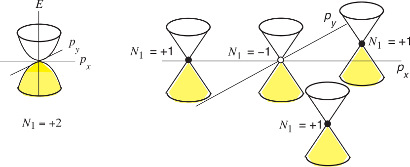
Figure 1: $Z_{2}$-topology of Dirac points in bilayer graphene. left: Dirac point with quadratic spectrum characterized by topological invariant $N_{1}=2$. Since the topological invariant is trivial in $Z_{2}$ topology, such a spectrum is unstable towards the gap formation, or to splitting. right: Splitting to topologically stable Dirac points due to trigonal warping.

In Bernal graphite (ABAB… stacking) the geometry of the Dirac lines is essentially different from rhombohedral graphite, because Bernal graphite is the 3D extension of bilayer graphene with AB stacking. Let us hence start by describing the bilayer graphene with AB stacking.

Since in each graphene layer the topological charges are $N_{1}=+1$ and $N_{1}=-1$ in the two valleys, in bilayer graphene the charges are summed up giving rise to trivial topological charges $N_{1}=+2\equiv 0$ and $N_{1}=-2\equiv 0$. Interaction between the layers may lead to several possible scenarios of the geometry of the fermionic spectrum in bilayer graphene:

1. If there is some special symmetry, such as the fundamental Lorentz invariance, one obtains a doubly degenerate conical spectrum. However, in bilayer graphene there is no symmetry which could support such a scenario.

2. The topological charge $N_{1}=2$ gives rise to the Dirac fermions with parabolic energy spectrum near the Dirac point, $E=E_{0}\pm{\bf p}^{2}_{\perp}/2m$ (Fig. 1 left). Such a spectrum belongs to the trivial element of the group $Z_{2}$, that is why the neglected hopping elements destroy the parabolic spectrum. The Dirac point disappears, and finite gap (the Dirac mass) emerges.

3. The Dirac point with $N_{1}=+2$ splits into two Dirac points, each with $N_{1}=+1$ and with conical spectrum (see [12] for the relativistic 3+1 system). Such splitting, however, violates the hexagonal symmetry of graphene.

4. The splitting of the $N_{1}=+2$ Dirac point, which is consistent with the hexagonal symmetry, is in Fig. 1 right. The $N_{1}=+2$ Dirac point splits into four Dirac conical points: the central Dirac point has $N_{1}=-1$, while three others with $N_{1}=+1$ each are connected by the $C_{3}$ symmetry, see Fig. 1 right. This is called the trigonal warping. The topological charges $N_{1}=\pm 1$ belong to the nontrivial element of the group $Z_{2}$. That is why each Dirac point is topologically stable and is not destroyed by addition of the neglected hopping elements, if they obey the time reversal and sublattice symmetry.

The bilayer graphene chooses the scenario (iv) with the trigonal warping, [13, 14] which prohibits the annihilation of the Dirac point due to splitting into the topologically stable Dirac points with $N_{1}=\pm 1$. Altogether the Brillouin zone of the bilayer graphene contains 8 Dirac conical points.

3 From topology of bilayer graphene to Bernal graphite

The trigonal warping also stabilizes the Dirac lines in the Bernal graphite (ABAB… stacking). Altogether the Brillouin zone of the Bernal graphite contains 8 Dirac lines,[15, 16] which originate from 8 Dirac conical points of bilayer graphene. These Dirac lines have finite energy and live inside the Fermi surface of graphite.

However, the topologically stable Dirac lines appear only in a certain region of momenta $p_{z}$. Outside that region the scenario (ii) without the Dirac lines takes place. This means that there exists an exceptional point in the spectrum, at which four topologically stable Dirac lines merge together and annihilate each other. [15, 16] Such a point is a direct analog of the nexus, a point in the real space where the $Z_{2}$ or $Z_{4}$ topological defects merge and annihilate each other, see Fig. 2 top. [18]

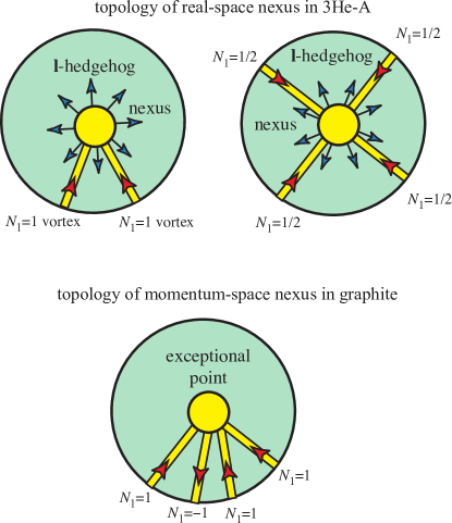
Figure 2: Real-space and momentum space nexus. top left: Real-space nexus in the dipole locked superfluid ³He-A, where vortices are described by $Z_{2}$-topology. Two vortices, with $N_{1}=1$ each, merge together at the hedgehog in the field of the orbital momentum vector $\hat{\bf l}$ and annihilate each other since $N_{1}=2\equiv 0$. top right: Real-space nexus in the dipole unlocked superfluid ³He-A, where vortices are described by $Z_{4}$-topology. Four half-quantum vortices, with $N_{1}=1/2$ each, merge together at the hedgehog and annihilate each other. bottom: Illustration of the topology of the momentum-space nexus in graphite. Dirac lines obey the $Z_{2}$-topology. Four Dirac lines, with $N_{1}=+1$, $N_{1}=+1$, $N_{1}=+1$ and $N_{1}=-1$, merge together at an exceptional point of the spectrum and annihilate each other, because $N_{1}=1+1+1-1=2\equiv 0$.

Let us find this exceptional point. According to $D_{6h}$ symmetry of graphite, the Dirac lines are situated in the vertical mirror planes, and thus the exceptional point is on the H-K-H line in the Brillouin zone at $p_{z}=P^{*}$.

The Hamiltonian of Bernal graphite is a 3D extension of the 2D Hamiltonian describing bilayer graphene:

$$H=\begin{pmatrix}\Delta&v_{F}pe^{-i\phi}&\gamma_{4}\Gamma(p_{z})v_{F}pe^{i\phi}&-2\gamma_{1}\Gamma(p_{z})\\ v_{F}pe^{i\phi}&\gamma_{2}(p_{z})&2\gamma_{3}\Gamma(p_{z})v_{F}pe^{-i\phi}&\gamma_{4}\Gamma(p_{z})v_{F}pe^{i\phi}\\ \gamma_{4}\Gamma(p_{z})v_{F}pe^{-i\phi}&2\gamma_{3}\Gamma(p_{z})v_{F}pe^{i\phi}&\gamma_{2}(p_{z})&v_{F}pe^{-i\phi}\\ -2\gamma_{1}\Gamma(p_{z})&\gamma_{4}\Gamma(p_{z})v_{F}pe^{-i\phi}&v_{F}pe^{i\phi}&\Delta\end{pmatrix}\,.$$ (2)

This corresponds to a rotated version of that written in Ref. [10] (we write the Hamiltonian in a basis spanned by the two layers $\times$ sublattice points, whereas Ref. [10] writes it in the eigenbasis defined by the strongest interlayer couplings), but we assume that the intralayer coupling $\gamma_{0}$ dominates over the other terms, and therefore also make the $\sigma\cdot p$ approximation for each layer. Here $pe^{i\phi}=p_{x}+ip_{y}$; $\Gamma(p_{z})=\cos((\pi/2a)p_{z})$, where $a$ is the distance between the K-point and H-point in the Brillouin zone of graphite and $p_{z}=0$ at the K-point so that $\Gamma(K)=1$ and $\Gamma(H)=0$. The function $\gamma_{2}(p_{z})=\gamma_{2}\Gamma^{2}(p_{z})/2$ describes the coupling across two layers and $\Delta$ denotes the locally broken A-B sublattice symmetry, which still preserves the global A-B symmetry. The coefficients $\gamma_{3,4}$ are related to the original tight-binding coefficients [10] $\tilde{\gamma}_{3,4}$ via $\gamma_{3,4}=\tilde{\gamma}_{3,4}/\gamma_{0}$. In graphite, $\gamma_{3}\approx 0.1$ and $\gamma_{4}\approx 0.01$ [17]. We neglect spin-orbit coupling and below we set $v_{F}=1$ for simplicity.

Hamiltonian (2) is invariant under time reversal symmetry (complex conjugation) combined with reflection from plane $p_{y}=0$ ($\phi\rightarrow-\phi$). This symmetry supports the $Z_{2}$ topology of Dirac points in graphene (Fig. 1 right) and Dirac lines in graphite.

4 Point of merging of Dirac lines

Since the merging point $P^{*}$ is on the H-K-H line, we consider the Hamiltonian at $p=0$ which has the following form (we consider only the traceless part):

$$\tilde{H}(p=0,p_{z})=H(p=0,p_{z})-\frac{1}{4}{\bf Tr}H(p=0,p_{z})=$$

$$\begin{pmatrix}f(p_{z})&0&0&-2g(p_{z})\\ 0&-f(p_{z})&0&0\\ 0&0&-f(p_{z})&0\\ -2g(p_{z})&0&0&f(p_{z})\end{pmatrix}~{},$$

$$f(p_{z})=\frac{1}{2}(\Delta-\gamma_{2}(p_{z})),~{}~{}g(p_{z})=\gamma_{1}\Gamma(p_{z})\,.$$ (3)

This can be rewritten in terms of the Pauli matrices $\sigma_{i}$ and $\tau_{i}$:

$$\tilde{H}(p=0,p_{z})=f(p_{z})\tau_{3}\sigma_{3}+g(p_{z})(\tau_{2}\sigma_{2}-\tau_{1}\sigma_{1})\,.$$ (4)

Let us introduce new matrices $\tilde{\tau}_{3}=-\tau_{3}$, $\tilde{\tau}_{1}=-\tau_{1}$, $\tilde{\tau}_{2}=\tau_{2}$ and the ”total spin” ${\bf J}=\frac{1}{2}({\mbox{\boldmath$\sigma$}}+\tilde{\mbox{\boldmath$\tau$}})$:

$$\tilde{H}(p=0,p_{z})=-(f(p_{z})+g(p_{z}))\tilde{\tau}_{3}\sigma_{3}+g(p_{z}){\mbox{\boldmath$\sigma$}}\cdot\tilde{\mbox{\boldmath$\tau$}}\,,$$ (5)

$${\mbox{\boldmath$\sigma$}}\cdot\tilde{\mbox{\boldmath$\tau$}}=2J(J+1)-3~{},~{}\tilde{\tau}_{3}\sigma_{3}=2J_{3}^{2}-1\,.$$ (6)

The Hamiltonian at $p=0$ can be expressed in terms of quantum numbers $J$ and $J_{3}$:

$$\tilde{H}(p=0)=-(f(p_{z})+g(p_{z}))(2J_{3}^{2}-1)+g(p_{z})(2J(J+1)-3)\,.$$ (7)

The exceptional point $p_{z}=P^{*}$ is at $f(p_{z})+g(p_{z})=0$, where three branches of the spectrum with $J=1$ are degenerate. Its position is determined by equation

$$\Delta-\gamma_{2}(p_{z})+2\gamma_{1}\Gamma(p_{z})=0\,.$$ (8)

In other notations this is the known equation for the exceptional point in graphite, see e.g. Ref. [16]. It is situated in the vicinity of the H-point. Away from this point, two branches with $J_{3}=\pm 1$ remain degenerate for all $p_{z}$. Close to the exceptional point

$$\tilde{H}(p=0,J=1)\approx-\lambda(p_{z}-P^{*})(2J_{3}^{2}-1)+g(P^{*})\,,$$ (9)

where $\lambda=f^{\prime}(P^{*})+g^{\prime}(P^{*})$.

The exceptional point $P^{*}$ is the merging point of four Dirac lines living in the symmetry planes at $p_{z}<P^{*}$. At $p_{H}>p_{z}>P^{*}$ the spectrum remains degenerate: the branches with $J_{3}=+1$ and $J_{3}=-1$ have the same energy. But these are the band contact lines rather than the Dirac lines: the branches have the same sign of energy counted from the line position, as distinct from $p_{z}<P^{*}$, where the touching branches have energies with opposite sign, which is the characteristics of a Dirac line (see Fig. 3). This means that at $p_{z}=P^{*}$ a band inversion occurs. The band inversion simultaneously happens for the branch with quantum numbers $J=1$ and $J_{3}=0$.

5 2D Dirac fermions at H-point

To see that the topology at $p_{H}>p_{z}>P^{*}$ is trivial, let us consider the $p_{x/y}$ plane containing the H-point. Since $\Gamma(p_{H})=0$, the Hamiltonian at the plane $p_{z}=p_{H}$ is

$$\tilde{H}(p,H)=\frac{1}{2}(\Delta-\gamma_{2}(p_{H}))\tau_{3}\sigma_{3}+p_{x}\sigma_{1}+p_{y}\sigma_{2}\,.$$ (10)

It represents two copies of massive 2D fermions with Dirac spectrum:

$$\tilde{E}(p)=\pm\sqrt{M^{2}+p^{2}}~{}~{},~{}~{}M=\frac{1}{2}(\Delta-\gamma_{2}(p_{H}))\,.$$ (11)

and thus two doubly degenerate branches. In addition to the contact line of $J_{z}=\pm 1$ branches, the other two branches, $J=1$, $J_{3}=0$ and $J=J_{3}=0$, contact each other. The Hamiltonian (10) has trivial $N_{1}$ topology. Due to continuity, the topology in the plane slightly below the H-point is also trivial. This demonstrates that at $p_{H}>p_{z}>P^{*}$ there are no Dirac lines. Instead there are band-contact lines, with trivial topological charge $N_{1}=0$. Thus the exceptional point $P^{*}$ is the point of merging of four Dirac lines.

6 Finite-energy Dirac lines

Let us consider the occurrence of the Dirac lines at a finite energy. For simplicity, we neglect $\gamma_{2}(p_{z})$ and $\gamma_{4}$, as they do not change the qualitative behavior of the Dirac lines close to the nexus. In this case, the characteristic equation for the bulk spectrum reads

$$(p^{2}+(\Delta-\epsilon)\epsilon)^{2}+(-4p^{3}\gamma_{3}^{2}(\Delta-\epsilon)^{2}-4\gamma_{1}^{2}\epsilon^{2}+8p^{3}\gamma_{1}\gamma_{3}\cos(3\phi))\Gamma^{2}(p_{z})+16p^{2}\gamma_{1}^{2}\gamma_{3}^{2}\Gamma(p_{z})^{4}=0.$$ (12)

This has four solutions for $\epsilon$. Let us analyze the solutions for three cases: (a) $|p_{z}|\ll P^{*}$, (b) $|p_{z}|=P^{*}$, and (c), $\pi/(2a)\geq|p_{z}|>P^{*}$. The relevant eigensolutions for a specific set of parameters in the three cases are plotted in Fig. 3.

For region (a), there are two eigenenergies $\epsilon\approx\pm\gamma_{1}\Gamma(p_{z})$, and two closer to zero. The latter two are plotted in Figs. 3(a,b) for a fixed $\Gamma(p_{z})$. Two low-energy solutions touch at specific points in the transverse momentum direction, either at $p=0$ and close to $\cos(3\phi)=-1$, $p=p_{0}=4\gamma_{1}\gamma_{3}\Gamma^{2}(p_{z})$, which is the exact position of the Dirac line for $\Delta=0$. For small $\Delta$, the Dirac lines at finite momentum obtain a finite energy $\epsilon=\Delta[1-1/(1+4\gamma_{3}^{2}\Delta\Gamma^{2}(p_{z}))]$ and slightly shift the line away from $p=p_{0}$. The Dirac line character however persists. Figure 3(c) shows all four eigenenergies in region (a). Here the splitting of the two low-energy lines is not visible as they are quite close to each other.

For $p_{z}=P^{*}$, the four solutions are plotted in Fig. 3(d). For low $\Delta$ and $p$, the energies are given by

$$\epsilon_{1,2}=\Delta\pm\sqrt{\Delta^{2}+p^{2}},\epsilon_{3,4}=\pm p.$$ (13)

There are hence two gapped and quadratic and two gapless linear branches, and three of them meet at $\epsilon=p=0$.

Above the nexus (region (c)), we may first set $\Gamma(p_{z})=0$, i.e., consider the $H$ point. There, the finite-energy solutions are given by (shifted by a constant energy from Eq. (11))

$$\epsilon_{a,b}=\frac{1}{2}(\Delta\pm\sqrt{4p^{2}+\Delta^{2}}),$$ (14)

The energies, plotted in Fig. 3(f), are doubly degenerate, but the degeneracy is lifted for a finite $\Gamma(p_{z})$, yielding two pairs of quadratic branches, the gap depending on the precise value of $\Gamma(p_{z})$. The lifting of this degeneracy is shown in Fig. 3(e).

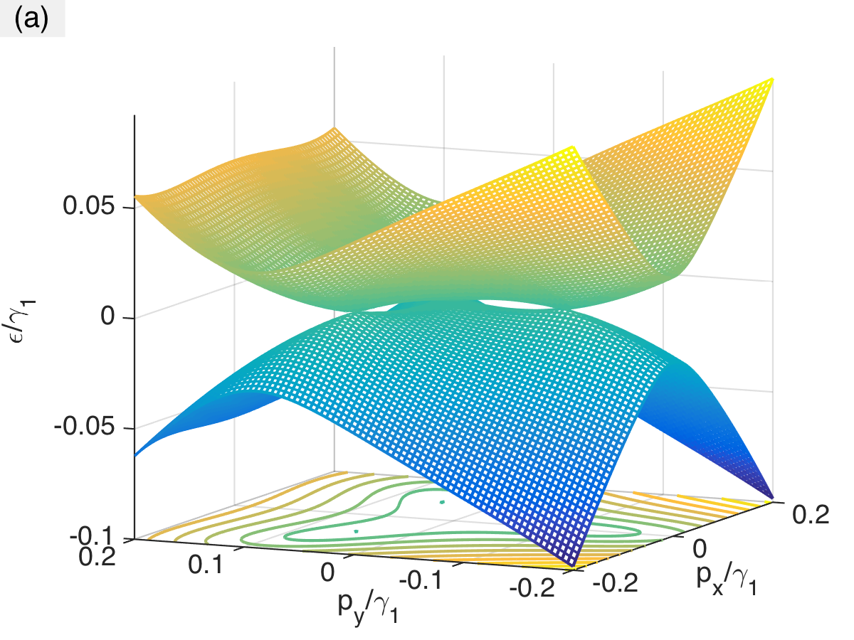
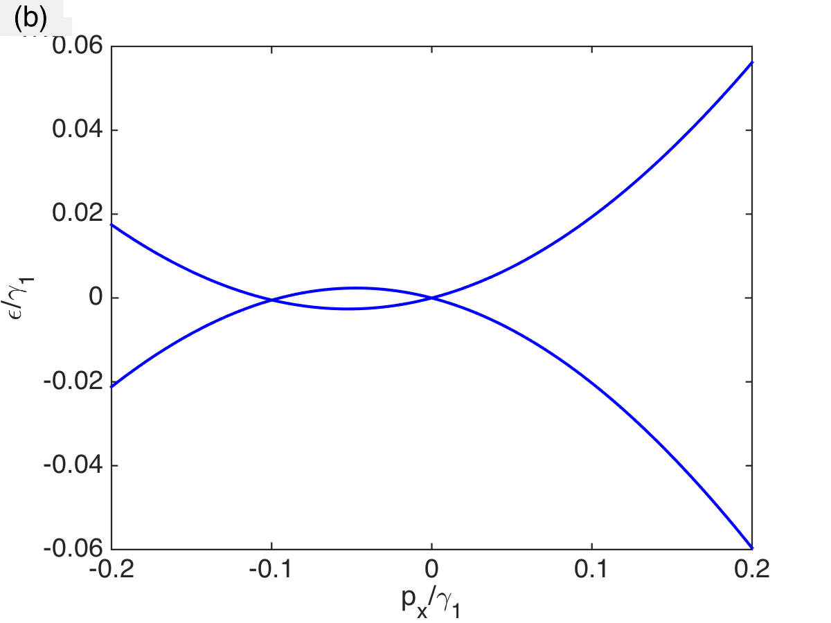
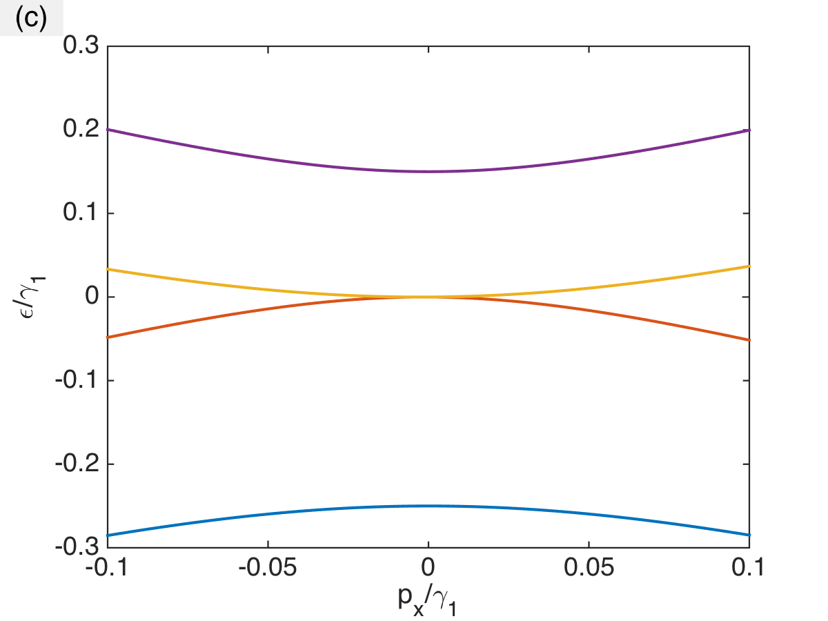
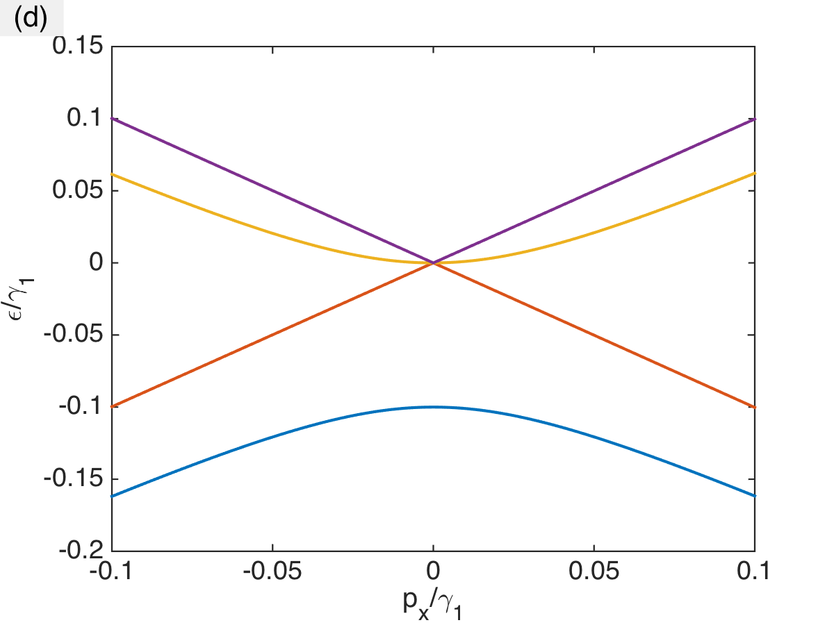
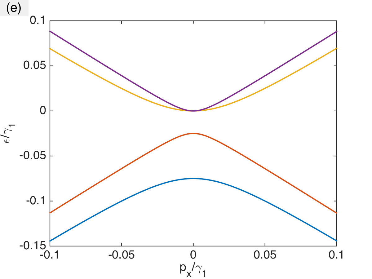
Figure 3: (a) Positions of the Dirac lines in the energy spectrum are seen as the points in momentum space where the two eigenenergies meet (plotted for $\Gamma(p_{z})=0.5$). (b) Cut through the $\phi=0$ axis revealing the positions of two of the Dirac lines. With a large $|\Delta|$ they shift towards lower values of $p$. (c) Same as previous but with $\Gamma(p_{z})=-2\Delta/\gamma_{1}$, showing also the higher-energy branches. Now the finite-momentum Dirac lines are too close to the center point to be visible. (d) Dispersion at the nexus, $\Gamma(p_{z})=-\Delta/(2\gamma_{1})$; (e) above the nexus, $\Gamma(p_{z})=-\Delta/(4\gamma_{1})$ and (f) at the $H$-point $\Gamma(p_{z})=0$. The figures are computed with $\Delta=-0.05\gamma_{1}$, $\gamma_{3}=0.1$, $\gamma_{2}=\gamma_{4}=0$.

7 Nexus

In the real space, the nexus is a kind of a Dirac monopole that terminates cosmic strings (the so-called $Z$-string in the Standard Model).[19] In chiral superfluid ³He-A the nexus is a hedgehog which terminates vortices with the $Z_{2}$ or $Z_{4}$ topology (Fig. 17.3 in the book [18] and Fig. 2 top). In the dipole-locked ³He-A the homotopy group for vortices is $Z_{2}$. That is why two vortices can terminate at the hedgehog in the field of the orbital momentum vector $\hat{\bf l}$, which is the analog of the Dirac magnetic monopole.

In the same manner the Dirac lines can be described by the $Z_{2}$ group, and if so, they may terminate on a Dirac monopole in some field. If the invariant $N_{1}$ belongs to the $Z_{2}$ group, which means that $N_{1}=2$ and $N_{1}=0$ are equivalent, then by some transformation of hopping elements the line described by even $N_{1}=2k$ can disappear. The lines with $N_{1}=\pm 1$ are stable. But when four such lines meet each other, their total charge is even, and thus they may annihilate each other. This also happens, since at $p_{z}>P^{*}$ the band contact lines are topologically trivial, $N_{1}=0$.

So, the point $p_{z}=P^{*}$ represents the nexus in momentum space, see Fig. 2 bottom. It is distinct from the 3D Weyl point in momentum space, which also represents the momentum-space analog of a Dirac monopole. Such a monopole contains the Dirac string: a singularity in the Berry phase which terminates at the monopole, see Fig. 11.4 in Ref. [18]. But this string is not observable.

8 Conclusion

The Dirac lines are suggested to exist in different semimetals. [20, 21, 22, 23, 24, 25, 26] The materials with Dirac lines are important, because they may have an (approximate) flat band on the boundary or at the interface between materials with different topological properties. The high density of states in the flat band provides a possible route to room-temperature superconductivity. [27]

However, the Bernal graphite is a very instructive example. Its spectrum demonstrates the possible interplay of several relevant topological invariants. One of them characterizes the local line element as in Ref. [2]. Another one is the global invariant, which characterizes for example the closed nodal ring as a whole: it is the same invariant which characterizes the 3D Dirac or Weyl point obtained by shrinking the nodal ring. There are also the topological invariants that characterize the Fermi surface(s). These include the local invariant of the Fermi surface [18] and the topology of the shape of the Fermi surface [28]. All this may combine to produce exotic topological patterns. The interplay of Weyl point and Fermi surface topologies with exchange of the Berry flux, when two Fermi surfaces contact each other, have been discussed in Refs. [29, 26]. The Bernal graphite provides an example of the interplay of Dirac lines in the mirror planes, an exceptional point (nexus), and Fermi surfaces with touching points between electron and hole pockets, see Refs. [15, 16].

References

References

- [1] J. von Neumann und E.P. Wigner, Über das Verhalten von Eigenwerten bei adiabatischen Prozessen, Phys. Zeit. 30, 467–470 (1929).
- [2] P. Hořava, Stability of Fermi surfaces and -theory, Phys. Rev. Lett. 95, 016405 (2005).
- [3] G.E. Volovik, The topology of quantum vacuum, Lecture Notes in Physics, 870, 343–383 (2013), arXiv:1111.4627.
- [4] S. Ryu and Y. Hatsugai, Topological origin of zero-energy edge states in particle-hole symmetric systems, Phys. Rev. Lett. 89, 077002 (2002).
- [5] A.P. Schnyder and S. Ryu, Topological phases and flat surface bands in superconductors without inversion symmetry, Phys. Rev. B 84, 060504(R) (2011).
- [6] A.P. Schnyder and P.M.R. Brydon, Topological surface states in nodal superconductors, J. Phys.: Condens. Matter 27 243201 (2015).
- [7] G.E. Volovik, Superconductivity with lines of gap nodes: Density of states in the vortex, JETP Lett. 58, 469–473 (1993).
- [8] T.T. Heikkilä and G.E. Volovik, Dimensional crossover in topological matter: Evolution of the multiple Dirac point in the layered system to the flat band on the surface, Pis’ma ZhETF 93, 63–68 (2011); JETP Lett. 93, 59–65 (2011); arXiv:1011.4185.
- [9] T.T. Heikkilä, N.B. Kopnin and G.E. Volovik, Flat bands in topological media, Pis’ma ZhETF 94, 252– 258 (2011); JETP Lett. 94, 233–239(2011); arXiv:1012.0905.
- [10] J.W. McClure, Band structure of graphite and de Haas-van Alphen effect, Phys. Rev. 108, 612-618 (1957).
- [11] D. Pierucci, H. Sediri, M. Hajlaoui, J.-C. Girard, T. Brumme, M. Calandra, E. Velez-Fort, G. Patriarche, M.G. Silly, G. Ferro, V. Souliere, M. Marangolo, F. Sirotti, F. Mauri, and A. Ouerghi, Evidence for flat bands near the Fermi level in epitaxial rhombohedral multilayer graphene, ACS Nano 9, 5432 (2015).
- [12] F.R. Klinkhamer and G.E. Volovik, Emergent CPT violation from the splitting of Fermi points, Int. J. Mod. Phys. A 20, 2795–2812 (2005); hep-th/0403037.
- [13] E. McCann and V.I. Fal’ko, Landau-level degeneracy and quantum Hall effect in a graphite bilayer, Phys. Rev. Lett. 96, 086805 (2006).
- [14] M. Koshino and T. Ando, Transport in bilayer graphene: Calculations within a self-consistent Born approximation, Phys. Rev. B 73, 245403 (2006).
- [15] G.P. Mikitik and Yu.V. Sharlai, Band-contact lines in the electron energy spectrum of graphite, Phys. Rev. B 73, 235112 (2006).
- [16] G.P. Mikitik and Yu.V. Sharlai, The Berry phase in graphene and graphite multilayers, Low Temp. Phys. 34, 794–780 (2008).
- [17] A.H. Castro Neto, F. Guinea, N.M.R. Peres, K.S. Novoselov, and A.K. Geim, The electronic properties of graphene, Rev. Mod. Phys. 81, 109 (2009).
- [18] G.E. Volovik, The Universe in a Helium Droplet (Oxford University Press, Oxford, UK, 2003).
- [19] J.M. Cornwall, Center vortices, nexuses, and the Georgi-Glashow model, Phys. Rev. D. 59, 125015 (1999).
- [20] H. Weng, Y. Liang, Q. Xu, Yu Rui, Z. Fang, Xi Dai, Y. Kawazoe, Topological node-line semimetal in three dimensional graphene networks, Phys. Rev. B 92, 045108 (2015).
- [21] L. S. Xie, L. M. Schoop, E. M. Seibel, Q. D. Gibson, W. Xie, and R. J. Cava, Potential ring of Dirac nodes in a new polymorph of Ca3P2, APL Mat. 3, 083602 (2015).
- [22] Youngkuk Kim, B.J. Wieder, C. L. Kane and A.M. Rappe, Dirac line nodes in inversion symmetric crystals, Phys. Rev. Lett. 115, 036806 (2015).
- [23] Yu Rui, H. Weng, Z. Fang, Xi Dai, and X. Hu, Topological node-line semimetal and Dirac semimetal state in antiperovskite Cu3PdN, Phys. Rev. Lett. 115, 036807 (2015).
- [24] K. Mullen, B. Uchoa, and D.T. Glatzhofer, Line of Dirac Nodes in Hyperhoneycomb Lattices, Phys. Rev. Lett. 115, 026403 (2015).
- [25] C. Fang, Y. Chen, H-Y. Kee, and L. Fu, Topological nodal line semimetals with and without spin-orbital coupling, arXiv:1506.03449.
- [26] D. Gosalbez-Martinez, I. Souza, D. Vanderbilt, Chiral degeneracies and Fermi-surface Chern numbers in bcc Fe, arXiv:1505.07727
- [27] T.T. Heikkilä and G.E. Volovik, Flat bands as a route to high-temperature superconductivity in graphite, arXiv:1504.05824.
- [28] S.P.Novikov and A.Ya.Maltsev, Topological phenomena in normal metals, Physics - Uspekhi, 41, 231–239 (1998).
- [29] F.R. Klinkhamer and G.E. Volovik, Emergent CPT violation from the splitting of Fermi points Int. J. Mod. Phys. A20, 2795–2812 (2005).