Local zeta regularization   and the scalar Casimir effect IV.   The case of a rectangular box

Davide Fermi$\,{}^{a}$, Livio Pizzocchero$\,{}^{b}$()

^a Dipartimento di Matematica, Università di Milano

Via C. Saldini 50, I-20133 Milano, Italy

e–mail: davide.fermi@unimi.it

^b Dipartimento di Matematica, Università di Milano

Via C. Saldini 50, I-20133 Milano, Italy

and Istituto Nazionale di Fisica Nucleare, Sezione di Milano, Italy

e–mail: livio.pizzocchero@unimi.it

Applying the general framework for local zeta regularization proposed in Part I of this series of papers, we compute the renormalized vacuum expectation value of several observables (in particular, of the stress-energy tensor and of the total energy) for a massless scalar field confined within a rectangular box of arbitrary dimension.

Keywords: Local Casimir effect, renormalization, zeta regularization.

AMS Subject classifications: 81T55, 83C47.

PACS: 03.70.+k, 11.10.Gh, 41.20.Cv .

1 Introduction.

In Part I of this series [12, 13, 14] we have considered in general local (and global) zeta regularization for a quantized neutral scalar field in a $d$-dimensional spatial domain $\Omega$, in the environment of $(d+1)$-dimensional Minkowski spacetime.

In the present Part IV we consider a massless field confined within a $d$-dimensional rectangular domain $\Omega=(0,a_{1})\times...\times(0,a_{d})$, with Dirichlet boundary conditions; applying the general scheme of Part I we renormalize several observables, namely: the vacuum expectation value (VEV) of the stress-energy tensor, the pressure on boundary points, the total energy VEV and of the total force acting on any side of the box. All these renormalized observables are represented as sums of series converging with exponential speed, for which we give quantitative remainder estimates. Our results hold for an arbitrary spatial dimension $d$; we subsequently specialize them to the subcase ($d=1$ and) $d=2$.

Let us make a comparison with the existing literature on the subject. The total energy and the forces on the sides of a rectangular box have been discussed in a lot of works, some of them using zeta regularization; here we only mention some of them. The foremost computation was performed by Lukosz [20, 21] for the electromagnetic field, by means of exponential regularization and Abel-Plana formula; the same technique was used by Mamaev and Trunov [22, 23] (also see [24, 25]) to discuss, amongst other models, the case of a conformal scalar field (). Alternative derivations of the total energy for a scalar field based on global zeta regularization were given by Ruggerio, Vilanni and Zimerman [31, 32] in two and three spatial dimensions, and by Ambjørn and Wolfram [3] (see also [4] for the electromagnetic case) in the case of a multidimensional rectangular cavity for several boundary conditions. The same configurations were later re-examined by X. Li, Cheng, J. Li and Zhai [19] by means of a zeta strategy, and by A. Edery [8, 9] using a so called “multidimensional cut-off technique”. Let us also cite the papers by Estrada, Fulling et al. [15, 16], on which we return later in this Introduction. Finally, let us mention the monographies of Elizalde et al. [10, 11] and Bordag et al. [5]; these can be taken as standard references for the study of global aspects.

In the present paper we consider global observables, such as the total energy and forces, mainly to complete the analysis of local aspects (i.e., the VEV of the stress-energy tensor), which occupy most of our analysis. Our series representations for these global observables are different, but equivalent to the ones of [5] (which appear to converge exponentially, like ours).

Concerning local aspects in the previous literature for a scalar field in a rectangular box let us first mention the two seminal papers [1] and [2] by Actor. In these papers $d=3$, the framework is Euclidean and the author renormalizes by analytic continuation the effective Lagrangian density and the VEV $\langle 0|\widehat{\phi}^{\,2}(x)|0\rangle$. The information contained in these works is equivalent, in the language of our papers, to the specification of the Dirichlet function $D_{s}({\bf x},{\bf y}):=\langle\delta_{\bf x}|(-\Delta)^{s}\delta_{\bf y}\rangle$ along the diagonal ${\bf y}={\bf x}$ (with $\Delta$ the Laplacian and ${\bf x},{\bf y}\in\Omega$), including its analytic continuation with respect to the complex parameter $s$. However, the VEV of the stress-energy tensor depends on $D_{s}({\bf x},{\bf x})$ as well as on the derivatives of $D_{s}({\bf x},{\bf y})$ with respect to ${\bf x}$ and ${\bf y}$, at points of the diagonal (see Part I of the present series). For this reason the results of [1, 2] are not sufficient to determine the stress-energy VEV, which in fact is not mentioned therein.

The renormalized VEV of the stress-energy tensor is derived in a work of Svaiter et al. [30]; the latter employs, again, analytic continuation methods in a formulation closely related to the approach of Actor. However, in [30] the authors consider an infinite rectangular waveguide, rather than a box; more precisely, it is assumed $d=3$ and the spatial domain is $\Omega=(0,a_{1})\times(0,a_{2})\times{\bf R}$. Apart from the domain, there are other differences bewteen the approach of Svaiter et al. and ours; in particular, the methods employed in [30] ultimately yield a representation of the stress-energy VEV via series converging with polynomial speed. Even though this approach could be extended to treat a box domain ($\Omega=(0,a_{1})\times(0,a_{2})\times(0,a_{3})$), it would most likely yield similar series representations, whose polynomial convergence would be slower compared to the exponential convergence of ours.

To go on, let us return to the already mentioned works by Estrada, Fulling et al. [15, 16]. Therein the configuration of a $2$-dimensional rectangular box is analysed for both Dirichlet and Neumann boundary conditions (along with some related models, such as the Casimir piston and the so-called “Casimir pistol”). The cited works introduce a regularized version of the stress-energy VEV, based on an exponential cutoff; this can be expressed in terms of the so-called cylinder kernel, which was also considered for other reasons in Parts I and II of this series. The regularized stress-energy VEV is computed by the method of images, allowing to express it as a sum over infinitely many optical paths. By integration of the above VEV, the authors of [15, 16] also obtain the regularized total energy and the regularized force acting on a side of the boundary. Their position of principle is that the theory with a cutoff is a more realistic description of the physical system under investigation; nonetheless, they also point out that the VEV of the observables for the system under analysis can be renormalized retaining only their regular parts with respect to the cut-off (an idea somehow related to what we call the “extended zeta approach”). Renormalization along these lines is carried out for global observables like the total energy, and hinted at for local observables (namely, for the energy density).

The present paper is organized as follows. In Section 2, as in the other papers of this series, we report a summary of results from Part I to be used in the present work. Section 3 and the related Appendices A, B, C are the core the paper; therein

we treat the box configuration $\Omega=(0,a_{1})\times...\times(0,a_{d})$ in arbitrary spatial dimension $d$, for Dirichlet boundary conditions. Our starting point is the heat kernel $\langle\delta_{\bf x}|e^{-\mathfrak{t}{\mathcal{A}}}\delta_{\bf y}\rangle$ for which we derive two different series representations capturing, respectively, the behavior for small and large $\mathfrak{t}$. As emphasized in Part I, the heat kernel determines an integral representation of the Dirichlet function $D_{s}({\bf x},{\bf y}):=\langle\delta_{\bf x}|(-\Delta)^{s}\delta_{\bf y}\rangle$, which can be used to construct the analytic continuation in $s$ of the latter. Combining these general facts with the series representation for the heat kernel cited above, we ultimately produce series expansions for the analytic continuations of $D_{s}({\bf x},{\bf y})$ and its derivatives, with the previously mentioned exponential speed of convergence; these determine all the local or global renormalized observables indicated before, from the stress-energy VEV to the force on each side of the box.

In Section 4, the previous general results are specialized to the cases with $d\in\{1,2\}$. For $d=1$, we recover from a different viewpoint the results already obtained in Section 6 of Part I where, as a first example of our general formalism, we discussed a massless scalar field on a segment $(0,a)$ (see this section of I for some references on this case, especially [26]). For $d=2$, working on $\Omega=(0,a_{1})\times(0,a_{2})$ and using the previously mentioned series expansions, we produce several graphs; some of them refer to the components of the stress-energy VEV for some choices of $a_{1},a_{2}$, while the others are about the further observables in which we are interested.Before moving on, let us mention that many of the results presented in this paper have been derived with the aid of the software $\tt{Mathematica}$ for both symbolic and numerical computations.

2 A summary of results from Part I

2.1   General setting.

Throughout the paper we use natural units, so that

$$c=1~{},\qquad\hbar=1~{}.$$ (2.1)

Our approach works in $(d+1)$-dimensional Minkowski spacetime, which is identified with ${\bf R}^{d+1}$ using a set of inertial coordinates

$$x=(x^{\mu})_{\mu=0,1,...,d}\equiv(x^{0},{\bf x})\equiv(t,{\bf x})~{};$$ (2.2)

the Minkowski metric is $(\eta_{\mu\nu})=\mbox{diag}(-1,1,...\,,1)$ . We fix a spatial domain $\Omega\subset{\bf R}^{d}$ and a background static potential $V\!:\!\Omega\!\to\!{\bf R}$. We consider a quantized neutral, scalar field $\widehat{\phi}:{\bf R}\times\Omega\to{\mathcal{L}}_{sa}(\mathfrak{F})$ ($\mathfrak{F}$ is the Fock space and ${\mathcal{L}}_{sa}(\mathfrak{F})$ are the selfadjoint operators on it); suitable boundary conditions are prescribed on $\partial\Omega$. The field equation reads

$$0=(-\partial_{tt}+\Delta-V({\bf x}))\widehat{\phi}({\bf x},t)$$ (2.3)

($\Delta:=\sum_{i=1}^{d}\partial_{ii}$ is the $d$-dimensional Laplacian). We put

$${\mathcal{A}}:=-\Delta+V~{},$$ (2.4)

keeping into account the boundary conditions on $\partial\Omega$, and consider the Hilbert space $L^{2}(\Omega)$ with inner product $\langle f|g\rangle:=\int_{\Omega}d{\bf x}\,\overline{f}({\bf x})g({\bf x})$. We assume ${\mathcal{A}}$ to be selfadjoint in $L^{2}(\Omega)$ and strictly positive (i.e., with spectrum $\sigma({\mathcal{A}})\subset[\varepsilon^{2},+\infty)$ for some $\varepsilon>0$).

We often refer to a complete orthonormal set $(F_{k})_{k\in{\mathcal{K}}}$ of (proper or improper) eigenfunctions of ${\mathcal{A}}$ with eigenvalues $(\omega^{2}_{k})_{k\in{\mathcal{K}}}$ ($\omega_{k}\!\geqslant\!\varepsilon$ for all $k\!\in\!{\mathcal{K}}$). Thus

$$\begin{split}&F_{k}:\Omega\to{\bf C};\qquad{\mathcal{A}}F_{k}=\omega^{2}_{k}F_{k}~{};\\ &\langle F_{k}|F_{h}\rangle=\delta(k,h)\quad\mbox{for all $k,h\in{\mathcal{K}}$}~{}.\end{split}$$ (2.5)

The labels $k\!\in\!{\mathcal{K}}$ can include both discrete and continuous parameters; $\int_{\mathcal{K}}dk$ indicates summation over all labels and $\delta(h,k)$ is the Dirac delta function on ${\mathcal{K}}$.

We expand the field $\widehat{\phi}$ in terms of destruction and creation operators corresponding to the above eigenfunctions, and assume the canonical commutation relations; $|0\rangle\in\mathfrak{F}$ is the vacuum state and VEV stands for “vacuum expectation value”.

The quantized stress-energy tensor reads ($\xi\!\in\!{\bf R}$ is a parameter)

$$\widehat{T}_{\mu\nu}:=\left(1-2\xi\right)\partial_{\mu}\widehat{\phi}\circ\partial_{\nu}\widehat{\phi}-\left({1\over 2}-2\xi\right)\eta_{\mu\nu}(\partial^{\lambda}\widehat{\phi}\,\partial_{\lambda}\widehat{\phi}+V\widehat{\phi}^{2})-2\xi\,\widehat{\phi}\circ\partial_{\mu\nu}\widehat{\phi}\,;$$ (2.6)

in the above we put $\widehat{A}\circ\widehat{B}:=(1/2)(\widehat{A}\widehat{B}+\widehat{B}\widehat{A})$ for all $\widehat{A},\widehat{B}\in{\mathcal{L}}_{sa}(\mathfrak{F})$, and all the bilinear terms in the field are evaluated on the diagonal (e.g., $\partial_{\mu}\widehat{\phi}\circ\partial_{\nu}\widehat{\phi}$ indicates the map $x\mapsto\partial_{\mu}\widehat{\phi}(x)\circ\partial_{\nu}\widehat{\phi}(x)$). The VEV $\langle 0|\widehat{T}_{\mu\nu}|0\rangle$ is typically divergent.

2.2   Zeta regularization.

The zeta-regularized field operator is

$$\widehat{\phi}^{u}:=(\kappa^{-2}{\mathcal{A}})^{-u/4}\widehat{\phi}~{},$$ (2.7)

where ${\mathcal{A}}$ is the operator (2.4), $u\in{\bf C}$ and $\kappa>0$ is a “mass scale” parameter; note that $\widehat{\phi}^{u}|_{u=0}=\widehat{\phi}$, at least formally. The zeta regularized stress-energy tensor is

$$\widehat{T}^{u}_{\mu\nu}:=(1\!-\!2\xi)\partial_{\mu}\widehat{\phi}^{u}\!\circ\partial_{\nu}\widehat{\phi}^{u}\!-\!\left({1\over 2}\!-\!2\xi\!\right)\!\eta_{\mu\nu}\!\left(\!\partial^{\lambda}\widehat{\phi}^{u}\partial_{\lambda}\widehat{\phi}^{u}\!+\!V(\widehat{\phi}^{u})^{2}\right)-2\xi\,\widehat{\phi}^{u}\!\circ\partial_{\mu\nu}\widehat{\phi}^{u}\,.$$ (2.8)

The VEV $\langle 0|\widehat{T}^{u}_{\mu\nu}|0\rangle$ is well defined for $\Re u$ large enough (see the forthcoming subsection 2.5); moreover, in the region of definition it is an analytic function of $u$. The same can be said of many related observables (including global objects, such as the total energy VEV).

For any one of these observables, let us denote with ${\mathcal{F}}(u)$ its zeta-regularized version and assume this to be analytic for $u$ in a suitable domain ${\mathcal{U}}_{0}\subset{\bf C}$. The zeta approach to renormalization can be formulated in two versions.

i) Restricted version. Assume the map ${\mathcal{U}}_{0}\!\to\!{\bf C}$, $u\!\mapsto\!{\mathcal{F}}(u)$ to admit an analytic continuation (indicated with the same notation) to an open subset ${\mathcal{U}}\!\subset\!{\bf C}$ with ${\mathcal{U}}\!\ni\!0$ ; then we define the renormalized observables as

$${\mathcal{F}}_{ren}:={\mathcal{F}}(0)~{}.$$ (2.9)

ii) Extended version. Assume that there exists an open subset ${\mathcal{U}}\!\subset\!{\bf C}$ with ${\mathcal{U}}_{0}\!\subset\!{\mathcal{U}}$, such that $0\!\in\!{\mathcal{U}}$ and the map $u\!\in\!{\mathcal{U}}_{0}\mapsto{\mathcal{F}}(u)$ has an analytic continuation to ${\mathcal{U}}\!\setminus\!\{0\}$ (still denoted with ${\mathcal{F}}$). Starting from the Laurent expansion ${\mathcal{F}}(u)=\sum_{k=-\infty}^{+\infty}{\mathcal{F}}_{k}u^{k}$, we introduce the regular part $(RP\,{\mathcal{F}})(u):=\sum_{k=0}^{+\infty}{\mathcal{F}}_{k}u^{k}$ and define

$${\mathcal{F}}_{ren}:=(RP\,{\mathcal{F}})(0)~{}.$$ (2.10)

Of course, if ${\mathcal{F}}$ is regular at $u=0$ the defnitions (2.9) (2.10) coincide.

Differently from the other papers of this series, the observables considered in the present Part IV will never exhibit singularities at $u=0$; thus, we will never need to use the prescription (ii).

In the sequel we will often refer to the stress-energy VEV, for which the prescription (i) gives

$$\langle 0|\widehat{T}_{\mu\nu}(x)|0\rangle_{ren}:=\langle 0|\widehat{T}^{u}_{\mu\nu}(x)|0\rangle\Big{|}_{u=0}~{}.$$ (2.11)

2.3   Conformal and non-conformal parts of the stress-energy VEV.

These are indicated by the superscripts $(\lozenge)$ and $(\blacksquare)$, respectively; they are defined by

$$\langle 0|\widehat{T}_{\mu\nu}|0\rangle_{ren}=\langle 0|\widehat{T}^{(\lozenge)}_{\mu\nu}|0\rangle_{ren}+(\xi\!-\!\xi_{d})\,\langle 0|\widehat{T}^{(\blacksquare)}_{\mu\nu}|0\rangle_{ren}~{},$$ (2.12)

where we are considering for the parameter $\xi$ the critical value

$$\xi_{d}:={d\!-\!1\over 4d}~{}.$$ (2.13)

2.4   Integral kernels.

If ${\mathcal{B}}$ is a linear operator in $L^{2}(\Omega)$, its integral kernel is the (generalized) function $({\bf x},{\bf y})\in\Omega\!\times\!\Omega\mapsto{\mathcal{B}}({\bf x},{\bf y}):=\langle\delta_{{\bf x}}|{\mathcal{B}}\,\delta_{{\bf y}}\rangle$ ($\delta_{\bf x}$ is the Dirac delta at ${\bf x}$). The trace of ${\mathcal{B}}$, assuming it exists, fulfills $\mbox{Tr}\,{\mathcal{B}}=\int_{\Omega}d{\bf x}\,{\mathcal{B}}({\bf x},{\bf x})$ .

In the following subsections ${\mathcal{A}}$ is a strictly positive selfadjoint operator in $L^{2}(\Omega)$, with a complete orthonormal set of eigenfunctions as in Eq. (2.5). In typical applications, ${\mathcal{A}}$ is the operator (2.4).

2.5   The Dirichlet kernel and its relations with the stress-energy VEV.

For (suitable) $s\in{\bf C}$, the $s$-th Dirichlet kernel of ${\mathcal{A}}$ is

$$D_{s}({\bf x},{\bf y}):={\mathcal{A}}^{-s}({\bf x},{\bf y})=\int_{\mathcal{K}}{dk\over\omega_{k}^{2s}}\;F_{k}({\bf x})\overline{F_{k}}({\bf y})~{}.$$ (2.14)

If $\Omega$ is a bounded domain with smooth boundary $\partial\Omega$ and ${\mathcal{A}}=-\Delta+V$ (with $V$ a smooth potential) is a strictly positive operator on $L^{2}(\Omega)$, considering the closure $\overline{\Omega}:=\Omega\cup\partial\Omega$ one can show that the map $D_{s}(~{},~{}):\overline{\Omega}\times\overline{\Omega}\to{\bf C}$, $({\bf x},{\bf y})\mapsto D_{s}({\bf x},{\bf y})$ is continuous along with all its partial derivatives up to order $j\in{\bf N}$, for all $s\in{\bf C}$ with $\Re s>d/2+j/2$ ; moreover, the eigenfunction expansion in Eq. (2.14) converges absolutely and uniformly on $\overline{\Omega}$ with all the derivatives up order $j$ for $\Re s>d+j/2$. Recalling Eq. (2.8), the regularized stress-energy VEV can be expressed as follows:

$${~{}}\langle 0|\widehat{T}^{u}_{00}({\bf x})|0\rangle\!=\!\kappa^{u}\!\!\left[\!\left(\!\frac{1}{4}\!+\!\xi\!\right)\!\!D_{{u-1\over 2}}({\bf x},{\bf y})\!+\!\left(\!\frac{1}{4}\!-\!\xi\!\right)\!\!(\partial^{x^{\ell}}\!\partial_{y^{\ell}}\!+\!V({\bf x}))D_{{u+1\over 2}}({\bf x},{\bf y})\right]_{{\bf y}={\bf x}}\!,$$ (2.15)

$$\langle 0|\widehat{T}^{u}_{0j}({\bf x})|0\rangle=\langle 0|\widehat{T}^{u}_{j0}({\bf x})|0\rangle=0~{},$$ (2.16)

$$\begin{split}&{~{}}\hskip 108.12054pt\langle 0|\widehat{T}^{u}_{ij}({\bf x})|0\rangle=\langle 0|\widehat{T}^{u}_{ji}({\bf x})|0\rangle=\\ &=\kappa^{u}\!\left[\!\Big{(}{1\over 4}-\xi\Big{)}\delta_{ij}\Big{(}\!D_{{u-1\over 2}}({\bf x},{\bf y})-(\partial^{\,x^{\ell}}\!\partial_{y^{\ell}}\!+\!V({\bf x}))D_{{u+1\over 2}}({\bf x},{\bf y})\Big{)}\,+\right.\\ &\hskip 142.26378pt\left.+\left(\!\Big{(}{1\over 2}-\xi\Big{)}\partial_{x^{i}y^{j}}-\xi\,\partial_{x^{i}x^{j}}\!\right)\!D_{{u+1\over 2}}({\bf x},{\bf y})\right]_{{\bf y}={\bf x}}\end{split}$$ (2.17)

($\langle 0|\widehat{T}^{u}_{\mu\nu}({\bf x})|0\rangle$ is short for $\langle 0|\widehat{T}^{u}_{\mu\nu}(t,{\bf x})|0\rangle$; indeed, the VEV does not depend on $t$). Of course, the map $\Omega\to{\bf C}$, ${\bf x}\mapsto\langle 0|\widehat{T}^{u}_{\mu\nu}({\bf x})|0\rangle$ possesses the same regularity as the functions ${\bf x}\in\Omega\mapsto D_{u\pm 1\over 2}({\bf x},{\bf x}),\partial_{zw}D_{u+1\over 2}({\bf x},{\bf x})$ ($z,w$ any two spatial variables); so, due to the previously mentioned results, ${\bf x}\mapsto\langle 0|\widehat{T}^{u}_{\mu\nu}({\bf x})|0\rangle$ is continuous on $\overline{\Omega}$ for $\Re u>d+1$.

Assume that $D_{u-1\over 2}$ and $\partial_{zw}D_{u+1\over 2}$ (for $z,w$ any two spatial variables) have analytic continuations regular at $u=0$ (which happens for the configuration considered in this paper); then, we can define

$$D_{\pm{1\over 2}}({\bf x},{\bf y}):=D_{u\pm 1\over 2}({\bf x},{\bf y})\Big{|}_{u=0}\,,$$ (2.18)

$$\partial_{zw}D_{{1\over 2}}({\bf x},{\bf y}):=\partial_{zw}D_{u+1\over 2}({\bf x},{\bf y})\Big{|}_{u=0}\,.$$ (2.19)

The renormalized stress-energy VEV $\langle 0|\widehat{T}_{\mu\nu}({\bf x})|0\rangle_{ren}:=\langle 0|\widehat{T}^{u}_{\mu\nu}({\bf x})|0\rangle|_{u=0}$ (see Eq. (2.11)) can be expressed as

$${~{}}\langle 0|\widehat{T}_{00}({\bf x})|0\rangle_{ren}\!=\!\left[\!\left(\!\frac{1}{4}\!+\!\xi\!\right)\!D_{\!-{1\over 2}}({\bf x},{\bf y})\!+\!\left(\!\frac{1}{4}\!-\!\xi\!\right)\!(\partial^{x^{\ell}}\!\partial_{y^{\ell}}\!+\!V({\bf x}))D_{\!+{1\over 2}}({\bf x},{\bf y})\right]_{{\bf y}={\bf x}}\!,\!$$ (2.20)

$$\langle 0|\widehat{T}_{0j}({\bf x})|0\rangle_{ren}=\langle 0|\widehat{T}_{j0}({\bf x})|0\rangle_{ren}=0~{},$$ (2.21)

$$\begin{split}&\hskip 116.65646pt\langle 0|\widehat{T}_{ij}({\bf x})|0\rangle_{ren}=\langle 0|\widehat{T}_{ji}({\bf x})|0\rangle_{ren}=\\ &=\!\left[\!\Big{(}{1\over 4}-\xi\Big{)}\delta_{ij}\Big{(}\!D_{\!-{1\over 2}}({\bf x},{\bf y})-(\partial^{\,x^{\ell}}\!\partial_{y^{\ell}}\!+\!V({\bf x}))D_{\!+{1\over 2}}({\bf x},{\bf y})\Big{)}\,+\right.\\ &\hskip 153.6447pt\left.+\left(\!\Big{(}{1\over 2}-\xi\Big{)}\partial_{x^{i}y^{j}}-\xi\,\partial_{x^{i}x^{j}}\!\right)\!D_{\!+{1\over 2}}({\bf x},{\bf y})\right]_{{\bf y}={\bf x}}.\end{split}$$ (2.22)

(More generally, in presence of a singularity at $u=0$ we should consider the regular parts of the functions $\kappa^{u}D_{u-1\over 2}$, $\kappa^{u}\partial_{zw}D_{u+1\over 2}$).

2.6   The heat kernel.

For $\mathfrak{t}\in[0,+\infty)$, this is given by

$$K(\mathfrak{t}\,;{\bf x},{\bf y}):=e^{-\mathfrak{t}{\mathcal{A}}}({\bf x},{\bf y})=\int_{\mathcal{K}}dk\;e^{-\mathfrak{t}\,\omega_{k}^{2}}\,F_{k}({\bf x})\overline{F_{k}}({\bf y})~{}.$$ (2.23)

If $\Omega$ is a bounded with smooth boundary $\partial\Omega$ and ${\mathcal{A}}=-\Delta+V$ ($V$ smooth) is strictly positive, the map $K(\mathfrak{t}\,;~{},~{}):\overline{\Omega}\times\overline{\Omega}\to{\bf C}$, $({\bf x},{\bf y})\mapsto K(\mathfrak{t}\,;{\bf x},{\bf y})$ is continuous along with all its partial derivatives of any order for all $\mathfrak{t}>0$ ; moreover, the eigenfunction expansion in Eq. (2.23) converges absolutely and uniformly (the same holds for all the corresponding derivatives).

2.7   The Dirichlet kernel as Mellin transform of the heat kernel.

For suitable values of $s\!\in\!{\bf C}$ (see Part I), there holds

$$D_{s}({\bf x},{\bf y})={1\over\Gamma(s)}\int_{0}^{+\infty}\!d\mathfrak{t}\;\mathfrak{t}^{s-1}\,K(\mathfrak{t}\,;{\bf x},{\bf y})~{}.$$ (2.24)

2.8   The case of product domains. Factorization of the heat kernel.

Let ${\mathcal{A}}:=-\Delta+V$ and consider the case where

$$\Omega=\Omega_{1}\times\Omega_{2}\ni{\bf x}=({\bf x}_{1},{\bf x}_{2})\,,{\bf y}=({\bf y}_{1},{\bf y}_{2})~{},$$ (2.25)

$$V({\bf x})=V_{1}({\bf x}_{1})+V_{2}({\bf x}_{2})$$ (2.26)

($\Omega_{a}\!\subset\!{\bf R}^{d_{a}}$ is an open subset, for $a\in\{1,2\}$; $d_{1}\!+\!d_{2}=d$); assume the boundary conditions on $\partial\Omega$ to arise from suitable boundary conditions prescribed separately on $\partial\Omega_{1}$ and $\partial\Omega_{2}$ so that, for $a=1,2$, the operators

$${\mathcal{A}}_{a}:=-\Delta_{a}+V({\bf x}_{a})$$ (2.27)

(with $\Delta_{a}$ the Laplacian on $\Omega_{a}$) are selfadjoint and strictly positive in $L^{2}(\Omega_{a})$. Then, the Hilbert space $L^{2}(\Omega)$ and the operator ${\mathcal{A}}$ can be represented as

$$L^{2}(\Omega)=L^{2}(\Omega_{1})\otimes L^{2}(\Omega_{2})~{},\qquad{\mathcal{A}}={\mathcal{A}}_{1}\otimes\mbox{{1}}+\mbox{{1}}\otimes{\mathcal{A}}_{2}~{}.$$ (2.28)

This implies, amongst else, that the heat kernels $K(\mathfrak{t}\,;{\bf x},{\bf y}):=e^{\mathfrak{t}{\mathcal{A}}}({\bf x},{\bf y})$, $K_{a}(\mathfrak{t}\,;{\bf x}_{a},{\bf y}_{a})$ $:=e^{\mathfrak{t}{\mathcal{A}}_{a}}({\bf x}_{a},{\bf y}_{a})$ ($a=1,2$) are related by

$$K(\mathfrak{t}\,;{\bf x},{\bf y})=K_{1}(\mathfrak{t}\,;{\bf x}_{1},{\bf y}_{1})\,K_{2}(\mathfrak{t}\,;{\bf x}_{1},{\bf x}_{2})~{}.$$ (2.29)

Similarly, writing $K(\mathfrak{t})$, $K_{a}(\mathfrak{t})$ ($a\in\{1,2\}$) for the heat traces of ${\mathcal{A}}$ and ${\mathcal{A}}_{a}$ ($a\in\{1,2\}$), respectively, we have

$$K(\mathfrak{t})=K_{1}(\mathfrak{t})\,K_{2}(\mathfrak{t})~{}.$$ (2.30)

The above considerations have obvious extensions to product domains with more than two factors.

2.9   Pressure on the boundary.

This is the force per unit area produced by the quantized field inside $\Omega$ at a point ${\bf x}\in\partial\Omega$. We first consider, for $\Re u$ large, the regularized pressure ${\bf p}^{u}({\bf x})$ with components

$$p^{u}_{i}({\bf x}):=\langle 0|\widehat{T}^{u}_{ij}({\bf x})|0\rangle\,n^{j}({\bf x})~{};$$ (2.31)

here and in the remainder of this paper, ${\bf n}({\bf x})\equiv(n^{i}({\bf x}))$ is the unit outher normal at ${\bf x}\in\partial\Omega$. For Dirichlet boundary conditions the above definition implies

$$p^{u}_{i}({\bf x})=\kappa^{u}\left[\left(\!-{1\over 4}\,\delta_{ij}\,\partial^{x^{\ell}}\!\partial_{y^{\ell}}+{1\over 2}\,\partial_{x^{i}y^{j}}\!\right)\!D_{u+1\over 2}({\bf x},{\bf y})\right]_{{\bf y}={\bf x}}n^{j}({\bf x})~{}.$$ (2.32)

We can define the renormalized pressure by analytic continuation as

$$p^{ren}_{i}({\bf x}):=p^{u}_{i}({\bf x})\Big{|}_{u=0}$$ (2.33)

(more generally, one should take the regular part if $u=0$ is a singular point; this will never happen in the present paper). Alternatively, we could put

$$p^{ren}_{i}({\bf x}):=\left(\lim_{{\bf x}^{\prime}\in\Omega,{\bf x}^{\prime}\to{\bf x}}\langle 0|\widehat{T}_{ij}({\bf x}^{\prime})|0\rangle_{ren}\right)n^{j}({\bf x})~{}.$$ (2.34)

Prescriptions (2.33) (2.34) do not always agree (for a counterexample, see Section 5 of Part II [13] of this series of papers). In Part I we conjectured that the two approaches agree when both of them give a finite result; this conjecture is true in the present case of a box as shown in subsection 3.6). Contrary to the previous works of this series [12, 13, 14], here we first discuss the pressure and next pass to the total energy; we make this choice because quite different computation techniques are employed for the stress-energy VEV and for the pressure, on the one hand, and for the total energy and integrated force, on the other hand.

2.10   The total energy.

The zeta-regularized total energy is

$${\mathcal{E}}^{u}:=\int_{\Omega}d{\bf x}\;\langle 0|\widehat{T}^{u}_{00}({\bf x})|0\rangle=E^{u}+B^{u}~{};$$ (2.35)

the second equality is proved after defining the regularized bulk and boundary energies, which are

$$E^{u}:={\kappa^{u}\!\over 2}\int_{\Omega}d{\bf x}\;D_{{u-1\over 2}}({\bf x},{\bf x})={\kappa^{u}\!\over 2}\;\mbox{Tr}\,\,{\mathcal{A}}^{{1-u\over 2}}~{},$$ (2.36)

$$B^{u}:=\kappa^{u}\left(\!{1\over 4}-\xi\!\right)\!\int_{\partial\Omega}\!da({\bf x})\,\left.{\partial\over\partial n_{{\bf y}}}\,D_{{u+1\over 2}}({\bf x},{\bf y})\right|_{{\bf y}={\bf x}}~{}.$$ (2.37)

One has $B^{u}=0$ for $\Omega$ bounded and either Dirichlet or Neummann boundary conditions on $\partial\Omega$.

Assuming the functions (2.36) (2.37) to be finite and analytic for suitable $u\in{\bf C}$, we define the renormalized energies by the restricted (or generalized) zeta approach; for example, we put

$$E^{ren}:=E^{u}\Big{|}_{u=0}$$ (2.38)

(again, if a singularity appears at $u=0$ we should take the regular part).

2.11   Forces on the boundary.

Let $\mathfrak{O}\!\subset\!\partial\Omega$; we consider (for $\Re u$ large) the regularized integrated force acting on $\mathfrak{O}$, i.e.,

$$\mathfrak{F}_{\mathfrak{O}}^{u}:=\int_{\mathfrak{O}}da({\bf x})\;{\bf p}^{u}({\bf x})$$ (2.39)

(${\bf p}^{u}({\bf x})$ is the regularized pressure of Eq. (2.31)). We can define the renormalized total force on $\mathfrak{O}$ as

$$\mathfrak{F}_{\mathfrak{O}}^{ren}:=\mathfrak{F}_{\mathfrak{O}}^{u}\Big{|}_{u=0}$$ (2.40)

(once more, the regular part should be taken if $u=0$ is a singular point, a variation which we shall never employ in the present paper). Alternatively, we could put

$$\mathfrak{F}_{\mathfrak{O}}^{ren}:=\int_{\mathfrak{O}}da({\bf x})\;{\bf p}^{ren}({\bf x})~{},$$ (2.41)

(${\bf p}^{ren}({\bf x})$ is the renormalized pressure, defined according to either Eq. (2.33) or Eq. (2.34)). In general the alternatives (2.40) (2.41) give different results.

3 The case of a massless field inside a box

3.1   Introducing the problem.

In the present section we analyse the model of a massless scalar field confined within a $d$-dimensional box, with no external potential; more precisely, we assume

$$\Omega=\times_{i=1}^{d}(0,a_{i})\quad\mbox{with $a_{i}>0$ for $i\in\{1,...,d\}$}~{},\qquad V=0~{}.$$ (3.1)

The boundary $\partial\Omega$ of the spatial domain is composed by the sides

$$\begin{split}&\pi_{p,\lambda}:=\{{\bf x}\in{\bf R}^{d}~{}|~{}\mbox{$x^{p}=\lambda\,a_{p}$\,, $x^{i}\in[0,a_{i}]$ for $i\neq p$}\}\\ &\hskip 48.36958pt\mbox{for $p\in\{1,...,d\}$, $\lambda\in\{0,1\}$}~{};\end{split}$$ (3.2)

for the sake of simplicity, we restrict attention to the case where the field fulfills Dirichlet boundary conditions on each one of these sides, meaning that

$$\widehat{\phi}(t,{\bf x})=0\quad\mbox{for all $t\in{\bf R}$, ${\bf x}\in\pi_{p,\lambda}$ ($p\in\{1,...,d\}$, $\lambda\in\{0,1\}$)}~{}.$$ (3.3)

As a matter of fact, all the results to be reported in the following could be generalized to the case of Neumann or periodic boundary conditions, possibly including cases where different boundary conditions are prescribed on different sides of the box; moreover, the methods to be presented could be adapted with little effort to deal with the cases of a massive scalar field ($V=m^{2}$) and of a slab configuration (see Part I) where

$$\Omega=\Omega_{1}\times{\bf R}^{d_{2}}\,,\quad\Omega_{1}=\times_{i=1}^{d_{1}}(0,a_{i})\;\subset\;{\bf R}^{d_{1}}\qquad(d_{1}+d_{2}=d)~{}.$$ (3.4)

None of these generalizations will be considered in the present paper.

3.2   The heat kernel.

Similarly to the model with a harmonic potential considered in our previous work [14], in the present setting we are dealing with a product domain configuration, in the sense of subsection 2.8. Working in standard Cartesian coordinates $(x^{i})_{i=1,...,d}$, the Hilbert space and the fundamental operator ${\mathcal{A}}:=-\Delta$ can berepresented as

$$L^{2}(\Omega)=\bigotimes_{i=1}^{d}L^{2}(0,a_{i})~{},$$ (3.5)

$$\begin{split}&{\mathcal{A}}={\mathcal{A}}_{1}\otimes\mbox{{1}}\otimes...\otimes\mbox{{1}}+...+\mbox{{1}}\otimes...\otimes\mbox{{1}}\otimes{\mathcal{A}}_{d}~{},\\ &\hskip 9.95863pt{\mathcal{A}}_{i}:=-{d^{2}\over dx^{2}}\quad\mbox{on $L^{2}(0,a_{i})$}\qquad(i\in\{1,...,d\})~{};\end{split}$$ (3.6)

for each operator ${\mathcal{A}}_{i}$ we assume the induced Dirichlet boundary conditions in $x^{i}=0$ and $x^{i}=a_{i}$ .

According to the general considerations of subsection 2.8 (see, in particular, Eq. (2.29)), in this situation the heat kernel associated to ${\mathcal{A}}$ factorizes; more precisely, we have

$$K(\mathfrak{t}\,;{\bf x},{\bf y})=\prod_{i=1}^{d}K_{i}(\mathfrak{t}\,;x^{i},y^{i})~{},$$ (3.7)

where, for $i\in\{1,...,d\}$, $K_{i}$ indicates the heat kernel of ${\mathcal{A}}_{i}$ . Hereafter we compute the heat kernels $K_{i}$, giving for all of them two distinct representations; these are suited to describe, respectively, the behaviour of the kernels $K_{i}$ for small and large $\mathfrak{t}$ (in a sense to be made more precise in the following) (). Clearly, each one of these representations yields, in turn, alternative expressions for the total heat kernel (3.7).   

3.2.1   First representation for the heat kernel (useful for large $\mathfrak{t}$).

Let us begin noting that, for any $i\in\{1,...,d\}$, a complete orthonormal set of eigenfunctions $(F_{k_{i}})_{k_{i}\in{\mathcal{K}}_{i}}$ for ${\mathcal{A}}_{i}$ in $L^{2}(0,a_{i})$, with corresponding eigenvalues $(\omega^{2}_{k_{i}})_{k_{i}\in{\mathcal{K}}_{i}}$, is given by

$$F_{k_{i}}(x^{i})\!:=\!\sqrt{2\over a_{i}}\,\sin(k_{i}x^{i})\,,\quad\!\omega^{2}_{k_{i}}:=k_{i}^{2}\quad\mbox{for }\,k_{i}\!\in\!{\mathcal{K}}_{i}\!\equiv\!\left\{{n_{i}\pi\over a_{i}}\,\Big{|}\,n_{i}=1,2,3,...\right\}.$$ (3.8)

Using the eigenfunction expansion (2.23), we obtain for the $1$-dimensional heat kernel $K_{i}$ the following expression ():

$$K_{i}(\mathfrak{t}\,;x^{i},y^{i})={2\over a_{i}}\sum_{n_{i}=1}^{+\infty}e^{-{n_{i}^{2}\pi^{2}\!\over a_{i}^{2}}\,\mathfrak{t}}\sin\!\Big{(}{n_{i}\pi\over a_{i}}\,y^{i}\Big{)}\sin\!\Big{(}{n_{i}\pi\over a_{i}}\,x^{i}\Big{)}~{}.$$ (3.9)

The above relation, along with Eq. (3.7), yields

$$K(\mathfrak{t}\,;{\bf x},{\bf y})={2^{d}\over a_{1}\,...\,a_{d}}\sum_{{\bf n}\in{\bf N}^{d}}e^{-\omega_{\bf n}^{2}\mathfrak{t}}\;C_{\bf n}({\bf x},{\bf y})~{},$$ (3.10)

where, for the sake of brevity, we put

$${\bf N}:=\{1,2,3,...\}~{},$$ (3.11)

$$\omega_{\bf n}^{2}:=\sum_{i=1}^{d}{n_{i}^{2}\pi^{2}\over a_{i}^{2}}~{},\quad C_{\bf n}({\bf x},{\bf y}):=\prod_{i=1}^{d}\sin\!\left({n_{i}\pi\over a_{i}}\,y^{i}\right)\!\sin\!\left({n_{i}\pi\over a_{i}}\,x^{i}\right)\quad\mbox{for ${\bf n}:=(n_{i})_{i=1,...,d}$}~{}.$$

Eq. (3.10) is easily seen to give a large $\mathfrak{t}$ expansion for the heat kernel $K(\mathfrak{t}\,;{\bf x},{\bf y})$ of ${\mathcal{A}}$; with this, we mean that the series over ${\bf n}\in{\bf N}^{d}$ in the cited equation is mainly determined by the terms corresponding to small values of $n_{i}$, for $i\in\{1,...,d\}$.

3.2.2   Second representation for the heat kernel (useful for small $\mathfrak{t}$).

Let us move on and note that, with little effort (namely, writing the sines in terms of complex exponentials), we can rephrase Eq. (3.9) as

$$K_{i}(\mathfrak{t}\,;x^{i},y^{i})={1\over 2a_{i}}\sum_{n_{i}=-\infty}^{+\infty}e^{-{n_{i}^{2}\pi^{2}\!\over a_{i}^{2}}\,\mathfrak{t}}\,\Big{[}e^{i{n_{i}\pi\over a_{i}}\,(x^{i}-y^{i})}-e^{i{n_{i}\pi\over a_{i}}\,(x^{i}+y^{i})}\Big{]}~{}.$$ (3.12)

Using the Poisson summation formula () and noting that

$$\begin{split}&\int_{-\infty}^{+\infty}\!\!\!dz\;e^{-{\pi^{2}\over a_{i}^{2}}\,\mathfrak{t}\,z^{2}}e^{i{\pi\over a_{i}}((x^{i}\pm y^{i})-2a_{i}h_{i})z}={a_{i}\over\sqrt{\pi\mathfrak{t}}}\;e^{-{(2a_{i}h_{i}-(x^{i}\pm y^{i}))^{2}\over 4\mathfrak{t}}}\\ &\hskip 48.36958pt\mbox{for\; $h_{i}\!\in\!{\bf Z}$\; with\; ${\bf Z}:=\{0,\pm 1,\pm 2,...\}$}~{},\end{split}$$ (3.13)

it follows from Eq. (3.12) that ()

$$K_{i}(\mathfrak{t}\,;x^{i},y^{i})={1\over\sqrt{4\pi\mathfrak{t}}}\sum_{h_{i}=-\infty}^{+\infty}\Big{[}e^{-{(2a_{i}h_{i}-(x^{i}-y^{i}))^{2}\over 4\mathfrak{t}}}-e^{-{(2a_{i}h_{i}-(x^{i}+y^{i}))^{2}\over 4\mathfrak{t}}}\Big{]}~{}.$$ (3.14)

The above identity can be rephrased as follows:

$$K_{i}(\mathfrak{t}\,;x^{i},y^{i})={1\over\sqrt{4\pi\mathfrak{t}}}\sum_{h_{i}\in{\bf Z},\,l_{i}\in\{1,2\}}\delta_{l_{i}}\;e^{-{1\over\mathfrak{t}}\,a_{i}^{2}(h_{i}-U_{l_{i}}(x^{i},y^{i}))^{2}}$$ (3.15)

where

$$\delta_{l_{i}}:=\left\{\!\!\begin{array}[]{cc}1&\mbox{for $l_{i}=1$}\\ -1&\mbox{for $l_{i}=2$}\end{array}\right.~{},\qquad U_{l_{i}}(x^{i},y^{i}):=\left\{\!\!\begin{array}[]{cc}{x^{i}-y^{i}\over 2a_{i}}&\mbox{for $l_{i}=1$}\\ {x^{i}+y^{i}\over 2a_{i}}&\mbox{for $l_{i}=2$}\end{array}\right.\!.$$ (3.16)

Eq. (3.15), along with Eq. (3.7), allows us to infer for the heat kernel the alternative representation

$$K(\mathfrak{t}\,;{\bf x},{\bf y})={1\over(4\pi\mathfrak{t})^{d/2}}\sum_{{\bf h}\in{\bf Z}^{d},\,{\bf l}\in\{1,2\}^{d}}\delta_{\bf l}\;e^{-{1\over\mathfrak{t}}\,b_{{\bf h}{\bf l}}({\bf x},{\bf y})}~{},$$ (3.17)

where, for simplicity of notation, we have put (recall Eq. (3.16))

$$\begin{split}&{\bf h}:=(h_{i})_{i=1,...,d}~{},\quad{\bf l}:=(l_{i})_{i=1,...,d}~{},\quad\delta_{\bf l}:=\prod_{i=1}^{d}\delta_{l_{i}}~{},\\ &\hskip 31.2982ptb_{{\bf h}{\bf l}}({\bf x},{\bf y}):=\sum_{i=1}^{d}a_{i}^{2}(h_{i}\!-\!U_{l_{i}}(x^{i},y^{i}))^{2}~{}.\end{split}$$ (3.18)

Notice that, for small $\mathfrak{t}$, the sum of the series appearing in Eq. (3.17) is mainly determined by the terms corresponding to small values of $|h_{i}|$, for $i\in\{1,...,d\}$; thus, the mentioned equation yields a small $\mathfrak{t}$ expansion for the heat kernel $K(\mathfrak{t}\,;{\bf x},{\bf y})$ .

3.2.3   Considerations on the sign of some coefficients.

Before moving on, let us emphasize a number of facts on the expansions (3.10) (3.17); we will resort to them in the following subsections, when performing the analytic continuation of the Dirichlet kernel and of its derivatives. i) On the one hand, we have

$$\omega_{\bf n}^{2}>0\quad\mbox{for all ${\bf n}\in{\bf N}^{d}$}~{}.$$ (3.19)

ii) On the other hand, notice that

$$b_{{\bf h}{\bf l}}({\bf x},{\bf y})\geqslant 0\quad\mbox{for all ${\bf h}\in{\bf Z}^{d}$, ${\bf l}\in\{1,2\}^{d}$, ${\bf x},{\bf y}\in\Omega$}~{}.$$ (3.20)

In particular, since

$$U_{l_{i}}(x^{i},y^{i})\in\left\{\!\begin{array}[]{cc}\left[-{1\over 2},{1\over 2}\right]&\mbox{for $l_{i}=1$}\\ \left[0,1\right]&\mbox{for $l_{i}=2$}\end{array}\right.$$ (3.21)

(see the definition of $U_{l_{i}}$ in Eq. (3.16)), it follows that

$$\begin{split}&\hskip 136.5733ptb_{{\bf h}{\bf l}}({\bf x},{\bf y})=0\quad\Leftrightarrow\\ &\Leftrightarrow\quad\mbox{for each $i\!\in\!\{1,...,d\}$\,, one has}~{}\left\{\!\!\begin{array}[]{ll}h_{i}=0,~{}l_{i}=1,~{}y^{i}=x^{i}\in[0,a_{i}]\\ \mbox{or}~{}h_{i}=0,~{}l_{i}=2,~{}y^{i}=x^{i}=0\\ \mbox{or}~{}h_{i}=1,~{}l_{i}=2,~{}y^{i}=x^{i}=a_{i}\end{array}\right.;\end{split}$$ (3.22)

let us stress that this implies, in particular, $b_{{\bf h}{\bf l}}({\bf x},{\bf y})\neq 0$ for ${\bf x}\neq{\bf y}$.

3.3   The Dirichlet kernel.

Consider the integral representation (2.24) for the Dirichlet kernel $D_{s}$ in terms of the heat kernel $K$ of ${\mathcal{A}}$ . We are going to construct the analytic continuation of $D_{s}$ in the style of Minakshisundaram (see [27]); to this purpose, let us fix arbitrarily

$$T\in(0,+\infty)$$ (3.23)

and re-express the cited integral representation as

$$D_{s}({\bf x},{\bf y})=D^{(>)}_{s}({\bf x},{\bf y})+D^{(<)}_{s}({\bf x},{\bf y})~{},\qquad\mbox{where}$$ (3.24)

$$D^{(>)}_{s}({\bf x},{\bf y}):={1\over\Gamma(s)}\int_{T}^{+\infty}\!d\mathfrak{t}\;\mathfrak{t}^{s-1}\,K(\mathfrak{t}\,;{\bf x},{\bf y})~{},$$ (3.25)

$$D^{(<)}_{s}({\bf x},{\bf y}):={1\over\Gamma(s)}\int_{0}^{T}d\mathfrak{t}\;\mathfrak{t}^{s-1}\,K(\mathfrak{t}\,;{\bf x},{\bf y})$$ (3.26)

(notice that $D^{(>)}_{s}$ and $D^{(<)}_{s}$ depend on $T$, but their sum $D_{s}$ does not!). The idea we are going to pursue in the following is to substitute into Eq.s (3.25) (3.26), respectively, the large and small $\mathfrak{t}$ expansions (3.10) (3.17) for the heat kernel $K$ ().

3.3.1   Series expansion and analytic continuation of $D^{(>)}_{s}({\bf x},{\bf y})$.

Using Eq.s (3.10) (3.25), we readily infer

$$D^{(>)}_{s}({\bf x},{\bf y})={2^{d}\over a_{1}...a_{d}\,\Gamma(s)}\sum_{{\bf n}\in{\bf N}^{d}}C_{\bf n}({\bf x},{\bf y})\int_{T}^{+\infty}\!\!d\mathfrak{t}\;\mathfrak{t}^{s-1}\,e^{-\omega_{\bf n}^{2}\mathfrak{t}}~{}.$$ (3.27)

Concerning the integral over $(T,+\infty)$, via the change of variable $\tau:=\omega_{\bf n}^{2}\mathfrak{t}$ (recall that $\omega_{\bf n}^{2}>0$ for all ${\bf n}\in{\bf N}^{d}$; see Eq. (3.19)), we obtain

$$\int_{T}^{+\infty}\!\!\!d\mathfrak{t}\;\mathfrak{t}^{s-1}\,e^{-\omega_{\bf n}^{2}\mathfrak{t}}=\omega_{\bf n}^{-2s}\!\int_{\omega_{\bf n}^{2}T}^{+\infty}\!\!\!d\tau\;\tau^{s-1}\,e^{-\tau}=\omega_{\bf n}^{-2s}\,\Gamma(s,\omega_{\bf n}^{2}\,T)\quad\mbox{for $s\!\in\!{\bf C}$}\,,$$ (3.28)

where the last passage contains the upper incomplete gamma function (see [29], p.174, Eq.8.2.2)

$$\Gamma(s,z):=\int_{z}^{+\infty}\!\!dw\;e^{-w}\,w^{s-1}\qquad(s\in{\bf C},\,z\in(0,+\infty))~{}.$$ (3.29)

Summing up, we have

$$D^{(>)}_{s}({\bf x},{\bf y})={2^{d}\over a_{1}...a_{d}\,\Gamma(s)}\sum_{{\bf n}\in{\bf N}^{d}}\omega_{\bf n}^{-2s}\,\Gamma(s,\omega_{\bf n}^{2}\,T)\;C_{\bf n}({\bf x},{\bf y})~{}.$$ (3.30)

The above expression can be used to evaluate derivatives of any order of the function $D^{(>)}_{s}({\bf x},{\bf y})$; for example, for any pair of spatial variables $z,w$, we obtain

$$\partial_{zw}D^{(>)}_{s}({\bf x},{\bf y})={2^{d}\over a_{1}...a_{d}\,\Gamma(s)}\sum_{{\bf n}\in{\bf N}^{d}}\omega_{\bf n}^{-2s}\,\Gamma(s,\omega_{\bf n}^{2}\,T)\;\partial_{zw}C_{\bf n}({\bf x},{\bf y})~{}.$$ (3.31)

Let us anticipate that the series in the right-hand sides of Eq.s (3.30) (3.31) converge for all $s\in{\bf C}$, even for ${\bf y}={\bf x}$ (see subsection 3.4 and Appendices A, C for more details); so, Eq.s (3.30) (3.31) yield automatically the analytic continuations of the maps $s\mapsto D^{(>)}_{s}({\bf x},{\bf y})$, $\partial_{zw}D^{(>)}_{s}({\bf x},{\bf y})$ to the whole complex plane.   

3.3.2   Series expansion and analytic continuation of $D^{(<)}_{s}({\bf x},{\bf y})$.

Proceeding similarly to what we did for the function $D_{s}^{(>)}({\bf x},{\bf y})$, we can use Eq.s (3.17) (3.26) to deduce

$$D^{(<)}_{s}({\bf x},{\bf y})={1\over(4\pi)^{d/2}\Gamma(s)}\sum_{{\bf h}\in{\bf Z}^{d},\,{\bf l}\in\{1,2\}^{d}}\delta_{\bf l}\int_{0}^{T}d\mathfrak{t}\;\mathfrak{t}^{s-{d\over 2}-1}\,e^{-{1\over\mathfrak{t}}\,b_{{\bf h}{\bf l}}({\bf x},{\bf y})}~{}.$$ (3.32)

To go on, for $\beta\geqslant 0$ and $s\in{\bf C}$ satisfying the conditions in the forthcoming Eq. (3.34), let us introduce the function

$${\mathcal{P}}_{s}(\beta):=\int_{0}^{1}d\tau\;\tau^{s-1}e^{-{\beta\over\tau}}~{};$$ (3.33)

it is easy to check that

$${\mathcal{P}}_{s}(\beta)=\left\{\!\begin{array}[]{ll}s^{-1}&\mbox{for $\beta=0$, $\Re s>0$}\\ \beta^{s}\,\Gamma(-s,\beta)&\mbox{for $\beta>0$}\end{array}\right.$$ (3.34)

where, again, $\Gamma(~{},~{})$ denotes the upper incomplete gamma function. Starting from Eq. (3.33), we find as well that

$$\partial_{\beta}^{\ell}{\mathcal{P}}_{s}(\beta)=(-1)^{\ell}\,{\mathcal{P}}_{s-\ell}(\beta)\quad\;\mbox{for all $\ell\in\{0,1,2,...\}$}~{}.$$ (3.35)

Let us return to Eq. (3.32) (recalling that $b_{{\bf h}{\bf l}}({\bf x},{\bf y})\geqslant 0$ for all ${\bf h}\in{\bf Z}^{d}$, ${\bf l}\in\{1,2\}^{d}$; see Eq. (3.20)) and make therein the change of variable $\tau:=\mathfrak{t}/T$; comparing with the definition (3.33) of ${\mathcal{P}}_{\bullet}(~{})$, we get

$$D^{(<)}_{s}({\bf x},{\bf y})={T^{s-{d\over 2}}\over(4\pi)^{d/2}\Gamma(s)}\sum_{{\bf h}\in{\bf Z}^{d},\,{\bf l}\in\{1,2\}^{d}}\delta_{\bf l}~{}{\mathcal{P}}_{s-{d\over 2}}\!\left({b_{{\bf h}{\bf l}}({\bf x},{\bf y})\over T}\right)\,.$$ (3.36)

The above result can be used, along with Eq. (3.35), to infer analogous representations for the derivatives of any order of $D^{(<)}_{s}$; for example, if $z,w$ are any two spatial variables, derivating term by term Eq. (3.36) we obtain

$$\partial_{zw}D^{(<)}_{s}({\bf x},{\bf y})=$$ (3.37)

$${T^{s-{d\over 2}-2}\over(4\pi)^{d/2}\Gamma(s)}\sum_{{\bf h}\in{\bf Z}^{d},\,{\bf l}\in\{1,2\}^{d}}\!\delta_{\bf l}\!\left[{\mathcal{P}}_{s-{d\over 2}-2}\!\left({b_{{\bf h}{\bf l}}\over T}\right)\!\partial_{z}b_{{\bf h}{\bf l}}\,\partial_{w}b_{{\bf h}{\bf l}}-T\,{\mathcal{P}}_{s-{d\over 2}-1}\!\!\left({b_{{\bf h}{\bf l}}\over T}\right)\!\partial_{zw}b_{{\bf h}{\bf l}}\right]\!({\bf x},{\bf y})~{}.$$

Let us point out that, due to the results reported in Eq. (3.22), we have

$$\begin{array}[]{cc}\mbox{$b_{{\bf h}{\bf l}}({\bf x},{\bf y})=0$ only for ${\bf y}={\bf x}$ and for}\\ \mbox{a finite number of terms in the series of Eq.s (\ref{DirInfExp}) (\ref{DzwDirInfExp})\,.}\end{array}$$ (3.38)

The above mentioned terms of Eq.s (3.36) (3.37) deserve special attention, and we must use the first equality in (3.34) to evaluate them; on the contrary, for the infinitely many terms with $b_{{\bf h}{\bf l}}({\bf x},{\bf y})>0$ , the second line in Eq. (3.34) gives expressions in terms of upper incomplete gamma functions. In this way we obtain

$$\begin{split}&\hskip 19.91684ptD^{(<)}_{s}({\bf x},{\bf y})={T^{s-{d\over 2}}\over(4\pi)^{d/2}\Gamma(s)(s-{d\over 2})}\left(\sum_{\begin{subarray}{c}{\bf h}\in{\bf Z}^{d},\,{\bf l}\in\{1,2\}^{d}\\ \mbox{\scriptsize{s.t.} }b_{{\bf h}{\bf l}}({\bf x},{\bf y})=0\end{subarray}}\delta_{\bf l}\right)+\\ &+\;{1\over(4\pi)^{d/2}\Gamma(s)}\sum_{\begin{subarray}{c}{\bf h}\in{\bf Z}^{d},\,{\bf l}\in\{1,2\}^{d}\\ \mbox{\scriptsize{s.t.} }b_{{\bf h}{\bf l}}({\bf x},{\bf y})>0\end{subarray}}\delta_{\bf l}\,\Bigg{(}b_{{\bf h}{\bf l}}^{s-{d\over 2}}\,\Gamma\!\left({d\over 2}\!-\!s\,,\,{b_{{\bf h}{\bf l}}\over T}\right)\!\!\Bigg{)}({\bf x},{\bf y})~{}.\end{split}$$ (3.39)

Let us repeat that the first sum in the above expression contains finitely many terms. Notice that the term in the first line of Eq. (3.39) is related to the first equality in Eq. (3.34) which, in principle, would require $\Re s>d/2$ ; however, this term makes sense for all complex $s$ except $s=d/2$ , where a simple pole appears. Moreover, the series in the second line of Eq.s (3.39) can be proved to converge for any complex $s$; we defer a comprehensive discussion of this statement to subsection 3.4 (see also Appendix A).

In view of the above remarks, Eq. (3.39) gives automatically the analytic continuation of $D^{(<)}_{s}({\bf x},{\bf y})$ to a meromorphic function of $s$ on the whole complex plane, with a simple pole singularity only at

$$s=d/2$$ (3.40)

for ${\bf x},{\bf y}$ such that the first sum in Eq. (3.41) is non-empty; this happens only for ${\bf y}={\bf x}$ due to Eq. (3.22). A similar analysis can be made for the derivatives of $D^{(<)}_{s}$. For example, if $z,w$ are any two spatial variables, we obtain the following expression from Eq. (3.37):

$$\begin{split}&\partial_{zw}D^{(<)}_{s}({\bf x},{\bf y})=-\,{T^{s-{d\over 2}-1}\over(4\pi)^{d/2}\Gamma(s)(s-{d\over 2}-1)}\,\Bigg{(}\sum_{\begin{subarray}{c}{\bf h}\in{\bf Z}^{d},\,{\bf l}\in\{1,2\}^{d}\\ \mbox{\scriptsize{s.t.} }b_{{\bf h}{\bf l}}({\bf x},{\bf y})=0\end{subarray}}\!\delta_{\bf l}\;\partial_{zw}b_{{\bf h}{\bf l}}({\bf x},{\bf y})\!\Bigg{)}\,+\!\\ &\hskip 8.5359pt+\,{1\over(4\pi)^{d/2}\Gamma(s)}\sum_{\begin{subarray}{c}{\bf h}\in{\bf Z}^{d},\,{\bf l}\in\{1,2\}^{d}\\ \mbox{\scriptsize{s.t.} }b_{{\bf h}{\bf l}}({\bf x},{\bf y})>0\end{subarray}}\!\delta_{\bf l}\left[b_{{\bf h}{\bf l}}^{s-{d\over 2}-2}\left(\Gamma\!\left({d\over 2}\!+\!2\!-\!s\,,{b_{{\bf h}{\bf l}}\over T}\right)\!\partial_{z}b_{{\bf h}{\bf l}}\,\partial_{w}b_{{\bf h}{\bf l}}\;+\right.\right.\\ &\hskip 170.71652pt\left.\left.-\;\Gamma\!\left({d\over 2}\!+\!1\!-\!s\,,{b_{{\bf h}{\bf l}}\over T}\right)\!b_{{\bf h}{\bf l}}\,\partial_{zw}b_{{\bf h}{\bf l}}\right)\right]\!({\bf x},{\bf y})~{}.\end{split}$$ (3.41)

Again, the first of the above two sums is made of finitely many terms; besides, contrary to what one could expect from Eq. (3.37), this sum contains no term with the first order derivatives $\partial_{w}b_{{\bf h}{\bf l}}({\bf x},{\bf y})$, $\partial_{z}b_{{\bf h}{\bf l}}({\bf x},{\bf y})$ because they vanish if $b_{{\bf h}{\bf l}}({\bf x},{\bf y})=0$. By considerations analogous to those made above for Eq. (3.39) (based on the convergence of the second sum for all $s\in{\bf C}$), we infer that Eq. (3.41) gives automatically the analytic continuation of $\partial_{zw}D^{(<)}_{s}({\bf x},{\bf y})$ to a meromorphic function of $s$ on the whole complex plane, with a simple pole singularity only for ${\bf y}={\bf x}$ at

$$s=d/2+1~{}.$$ (3.42)

Let us stress that Eq.s (3.39) (3.41) are just the original Eq.s (3.36) (3.37), rewritten separating the terms with $b_{{\bf h}{\bf l}}({\bf x},{\bf y})=0$ for a better understanding of the behaviour with respect to $s$ . In the sequel, even when considering meromorphic continuations, we will always refer to the more concise representations (3.36) (3.37).

3.3.3   Conclusions for the Dirichlet kernel.

Using Eq. (3.24) and expressions (3.30) (3.36) for the functions $D_{s}^{(>)}$, $D_{s}^{(<)}$, respectively, we obtain the analytic continuation of the full Dirichlet kernel $D_{s}({\bf x},{\bf y})$ to a meromorphic function on the whole complex plane. Similar results hold for the derivatives of the Dirichlet kernel (see Eq.s (3.31) (3.37)).

The only singularity of $D_{s}({\bf x},{\bf y})$ is a simple pole for

$${\bf y}={\bf x}\quad\mbox{and}\quad s=d/2~{},$$ (3.43)

while $\partial_{zw}D_{s}({\bf x},{\bf y})$ (for any pair of spatial variables $z,w$) has a simple pole for

$${\bf y}={\bf x}\quad\mbox{and}\quad s=d/2+1~{}.$$ (3.44)

In particular the analytic continuation of $D_{u-1\over 2}({\bf x},{\bf y})|_{{\bf y}={\bf x}}$ and $\partial_{zw}D_{u+1\over 2}({\bf x},{\bf y})|_{{\bf y}={\bf x}}$, required for the evaluation of the regularized stress-energy VEV and pressure, are both regular at $u=0$ .

3.4   Convergence and remainder estimates for the series in Eq.s (3.30) (3.31) and (3.36) (3.37).

This subject is discussed in more detail in Appendix A; here we only report the main results. In the mentioned Appendix we show that the series cited in the title of this subsection are absolutely convergent; moreover, we derive fully quantitative remainder estimates when these series are approximated by finite sums.

To report here these estimates we need some notations, introduced hereafter. First of all we put

$$\begin{split}&\hskip 36.98866pta:=\min_{i\in\{1,...,d\}}\{a_{i}\}~{},\qquad A:=\max_{i\in\{1,...,d\}}\{a_{i}\}~{};\\ &|{\bf z}|:=\left(\sum_{i=1}^{d}z_{i}^{2}\right)^{\!\!1/2}\qquad\mbox{for ${\bf z}={\bf n}\in{\bf N}^{d}$ or ${\bf z}={\bf h}\in{\bf Z}^{d}$}~{}.\end{split}$$ (3.45)

Besides, for $N\!\in\!(2\sqrt{d},+\infty)$, $\alpha\!\in\!(0,1)$, $\beta\!\in\!(0,+\infty)$, $\sigma,\rho\in{\bf R}$, we set

$$H^{(d)}_{N}(\alpha,\beta;\sigma,\rho):=$$ (3.46)

$${\pi^{d/2}\over(1\!-\!\alpha)^{\sigma}(\alpha\,\beta)^{{d+\rho\over 2}}\,\Gamma({d\over 2})}\left({N\!-\!\sqrt{d}\over N\!-\!2\sqrt{d}}\right)^{\!\!\!d-1}\!\Gamma(\sigma,(1\!-\!\alpha)\beta N^{2})\;\Gamma\!\left({d\!+\!\rho\over 2}\,;\alpha\,\beta(N\!-\!2\sqrt{d})^{2}\right)\,;$$

it can be shown that there holds the asymptotic expansion

$$\begin{split}&H^{(d)}_{N}(\alpha,\beta;\sigma,\rho)={\pi^{d/2}\,\beta^{\sigma-2}e^{-4\alpha\,\beta d}\over\alpha(1\!-\!\alpha)\,\Gamma({d\over 2})}\;\,e^{-\beta N(N-4\alpha\beta\sqrt{d})}N^{2\sigma+\rho+d-4}\,(1+O(N^{-1}))\\ &\hskip 162.18062pt\mbox{for $N\to+\infty$}~{}.\end{split}$$ (3.47)

Finally, we put

$$C_{a,A}^{(d)}(\sigma,N):=\max\left[\left(\!a\left(1\!-\!{\sqrt{d}\over N}\right)\!\right)^{\!\!\!2\sigma}\!,\left(\!A\left(1\!+\!{\sqrt{d}\over N}\right)\!\right)^{\!\!\!2\sigma}\right].$$ (3.48)

Having introduced the above notations, in the next two subsections we report the remainder estimates of Appendix A for the series expansions of $D_{s}^{(>)}$, $D_{s}^{(<)}$ and of their derivatives. In all cases the remainder is controlled by the function $H_{N}^{(d)}$; due to the exponential decay of this function for large $N$ (see Eq. (3.47)), good approximations of all the series under investigation can be obtained by just summing the first few terms.

3.4.1   Estimates for the series (3.30) (3.31).

Consider any $s\in{\bf C}$; keeping in mind Eq. (3.30), for any $N\in(0,+\infty)$ let us write

$$\begin{split}&\hskip 59.75095ptD^{(>)}_{s}({\bf x},{\bf y})=D^{(>)}_{s,N}({\bf x},{\bf y})+R^{(>)}_{s,N}({\bf x},{\bf y})~{},\\ &D^{(>)}_{s,N}({\bf x},{\bf y}):={2^{d}\over a_{1}...a_{d}\,\Gamma(s)}\sum_{{\bf n}\in{\bf N}^{d},\,|{\bf n}|\leqslant N}\omega_{\bf n}^{-2s}\,\Gamma(s,\omega_{\bf n}^{2}\,T)\;C_{\bf n}({\bf x},{\bf y})~{},\\ &R^{(>)}_{s,N}({\bf x},{\bf y}):={2^{d}\over a_{1}...a_{d}\,\Gamma(s)}\sum_{{\bf n}\in{\bf N}^{d},\,|{\bf n}|>N}\omega_{\bf n}^{-2s}\,\Gamma(s,\omega_{\bf n}^{2}\,T)\;C_{\bf n}({\bf x},{\bf y})~{}.\end{split}$$ (3.49)

This equation implies a similar representation for the (analytically continued) derivatives of $D^{(>)}_{s}$ in terms of the derivatives of $D^{(>)}_{s,N}$ and $R^{(>)}_{s,N}$ . For the remainder function $R^{(>)}_{s,N}({\bf x},{\bf y})$ and for its derivatives with respect to any two spatial variables $z,w$, we have the following uniform estimates:

$$\begin{split}&\hskip 21.33955pt\left|R^{(>)}_{s,N}({\bf x},{\bf y})\right|\leqslant{\max(a^{2\Re s},A^{2\Re s})\over a_{1}...a_{d}\,\pi^{2\Re s}|\Gamma(s)|}\;H^{(d)}_{N}\!\left(\alpha,{\pi^{2}\,T\over A^{2}}\,;\Re s,-2\Re s\right)\\ &\mbox{for either \quad$\Re s\!\geqslant\!0$, $N\!>\!2\sqrt{d}$}\qquad\mbox{or}\quad\mbox{$\Re s\!<\!0$, $\displaystyle{N\!>\!2\sqrt{d}\!+\!{A\over\pi}\sqrt{|\Re s|\over\alpha\,T}}$}~{};\end{split}$$ (3.50)

$$\begin{split}&\left|\partial_{zw}R^{(>)}_{s,N}({\bf x},{\bf y})\right|\leqslant{\max(a^{2\Re s},A^{2\Re s})\over a_{1}...a_{d}\,a^{2}\,\pi^{2(\Re s-1)}|\Gamma(s)|}\;H^{(d)}_{N}\!\left(\alpha,{\pi^{2}\,T\over A^{2}}\,;\Re s,2(1\!-\!\Re s)\right)\\ &\hskip 4.26773pt\mbox{for either \qquad$\Re s\!\geqslant\!1$, $N\!>\!2\sqrt{d}$}\quad\mbox{or}\quad\mbox{$\Re s\!<\!1$, $\displaystyle{N\!>\!2\sqrt{d}\!+\!{A\over\pi}\sqrt{(1\!-\!\Re s)\over\alpha\,T}}$}~{}.\end{split}$$ (3.51)

In the above, $\alpha$ is a parameter that can be freely chosen in $(0,1)$; of course, the best choice is the one minimizing the right-hand sides of Eq.s (3.50) and (3.51), which depends on the other parameters (e.g., $N,T$) involved in these considerations.

3.4.2   Estimates for the series (3.36) (3.37).

Let $s\in{\bf C}$, and exclude the case (3.43); keeping in mind Eq. (3.36), for any $N\in(0,+\infty)$ we put

$$\begin{split}&\hskip 62.59596ptD^{(<)}_{s}({\bf x},{\bf y})=D^{(<)}_{s,N}({\bf x},{\bf y})+R^{(<)}_{s,N}({\bf x},{\bf y})~{},\\ &D^{(<)}_{s,N}({\bf x},{\bf y}):={T^{s-{d\over 2}}\over(4\pi)^{d/2}\Gamma(s)}\sum_{{\bf h}\in{\bf Z}^{d},\,|{\bf h}|\leqslant N,\,{\bf l}\in\{1,2\}^{d}}\delta_{\bf l}\;{\mathcal{P}}_{s-{d\over 2}}\!\left({b_{{\bf h}{\bf l}}({\bf x},{\bf y})\over T}\right)~{},\\ &R^{(<)}_{s,N}({\bf x},{\bf y}):={T^{s-{d\over 2}}\over(4\pi)^{d/2}\Gamma(s)}\sum_{{\bf h}\in{\bf Z}^{d},\,|{\bf h}|>N,\,{\bf l}\in\{1,2\}^{d}}\delta_{\bf l}\;{\mathcal{P}}_{s-{d\over 2}}\!\left({b_{{\bf h}{\bf l}}({\bf x},{\bf y})\over T}\right)~{}.\end{split}$$ (3.52)

The above equation can be used to derive similar representations for the (analytically continued) derivatives of $D^{(<)}_{s}$ in terms of the derivatives of $D^{(<)}_{s,N}$ and $R^{(<)}_{s,N}$, with the exclusion of the case (3.44) . For the remainder function $R^{(<)}_{s,N}$ and for its derivatives with respect to any two spatial variables $z^{i},w^{j}$ ($i,j\in\{1,...,d\}$), we have the following uniform estimates:

$$\begin{split}&\left|R^{(<)}_{s,N}({\bf x},{\bf y})\right|\leqslant{C^{(d)}_{a,A}(\Re s-{d\over 2},N)\over\pi^{d/2}|\Gamma(s)|}\;H^{(d)}_{N}\!\left(\alpha,{a^{2}(1\!-\!{\sqrt{d}\over N})^{2}\over T}\,;{d\over 2}\!-\!\Re s,2\Re s\!-\!d\right)\\ &\mbox{for either \quad$\displaystyle{\Re s\!\leqslant\!{d\over 2}}$, $N\!>\!2\sqrt{d}$}\quad\mbox{or}\quad\mbox{$\displaystyle{\Re s\!>\!{d\over 2}}$, $\displaystyle{N\!>\!3\sqrt{d}\!+\!{1\over a}\sqrt{(\Re s\!-\!{d\over 2})T\over\alpha}}$}~{};\end{split}$$ (3.53)

$$\left|\partial_{z^{i}w^{j}}R^{(<)}_{s,N}({\bf x},{\bf y})\right|\leqslant$$ (3.54)

$$\begin{split}&{1\over\pi^{d/2}|\Gamma(s)|}\!\!\left[\!\left(\!1\!+\!{\sqrt{d}\over N}\!\right)^{\!\!2}\!\!A^{2}C_{a,A}^{(d)}\!\!\left(\!\Re s\!-\!{d\over 2}\!-\!2,N\!\right)\!H^{(d)}_{N}\!\!\left(\!\alpha,{a^{2}(1\!-\!{\sqrt{d}\over N})^{2}\over T};{d\over 2}\!+\!2\!-\!\Re s,2\Re s\!-\!d\!-\!2\!\right)\right.\\ &\hskip 11.38092pt\left.\phantom{\left(\!1\!+\!{\sqrt{d}\over N}\!\right)^{\!\!2}}+{1\over 2}\;\delta_{ij}\,C_{a,A}^{(d)}\!\!\left(\!\Re s\!-\!{d\over 2}\!-\!1,N\!\right)\!H^{(d)}_{N}\!\!\left(\!\alpha,{a^{2}(1\!-\!{\sqrt{d}\over N})^{2}\over T}\,;{d\over 2}\!+\!1\!-\!\Re s,2\Re s\!-\!d\!-\!2\!\right)\!\right]\end{split}$$

$$\mbox{for either \quad$\displaystyle{\Re s\!\leqslant\!{d\over 2}\!+\!1}$, $N\!>\!2\sqrt{d}$}\quad\mbox{or}\quad\mbox{$\displaystyle{\Re s\!>\!{d\over 2}\!+\!1}$, $\displaystyle{N\!>\!3\sqrt{d}\!+\!{1\over a}\sqrt{(\Re s\!-\!{d\over 2}\!-\!1)T\over\alpha}}$}~{}.$$

Again, the parameter $\alpha$ can be freely taken in $(0,1)$ and it is conventient to choose for it the value minimizing the right-hand sides of Eq.s (3.53) (3.54), keeping into account the choices made for the other parameters (in particular, $N$).

3.5   The stress-energy tensor.

Consider the representations deduced in subsection 3.3 for the analytic continuations of the Dirichlet kernel and of its derivatives. Resorting to Eq.s (2.15-2.17), we obtain the following expressions for the components of the regularized VEV of the stress-energy tensor:

$$\langle 0|\widehat{T}^{u}_{\mu\nu}({\bf x})|0\rangle=T^{u,(>)}_{\mu\nu}({\bf x})+T^{u,(<)}_{\mu\nu}({\bf x})~{},\qquad$$ (3.55)

where, for $\bullet$ equal to $>$ or $<$, $T^{u,(\bullet)}_{\mu\nu}({\bf x})$ has the espression corresponding to Eq.s (2.15-2.17), with $D_{s}$ replaced by $D^{(\bullet)}_{s}$. Thus, for $i,j\in\{1,...,d\}$, we have

$$T^{u,(\bullet)}_{00}({\bf x})=\kappa^{u}\!\left[\left(\!\frac{1}{4}+\xi\!\right)\!D^{(\bullet)}_{{u-1\over 2}}({\bf x},{\bf y})+\left(\!\frac{1}{4}-\xi\!\right)\!\partial^{x^{\ell}}\!\partial_{y^{\ell}}D^{(\bullet)}_{{u+1\over 2}}({\bf x},{\bf y})\right]_{{\bf y}={\bf x}},$$ (3.56)

$$T^{u,(\bullet)}_{0j}({\bf x})=T^{u,(\bullet)}_{j0}({\bf x})=0~{},$$ (3.57)

$$\begin{split}&T^{u,(\bullet)}_{ij}({\bf x})=\kappa^{u}\!\left[\!\left(\!{1\over 4}-\xi\!\right)\!\delta_{ij}\Big{(}\!D^{(\bullet)}_{{u-1\over 2}}({\bf x},{\bf y})-\partial^{\,x^{\ell}}\!\partial_{y^{\ell}}D^{(\bullet)}_{{u+1\over 2}}({\bf x},{\bf y})\Big{)}\,+\right.\\ &\hskip 142.26378pt\left.+\left(\!\Big{(}{1\over 2}-\xi\Big{)}\partial_{x^{i}y^{j}}-\xi\,\partial_{x^{i}x^{j}}\!\right)\!D^{(\bullet)}_{{u+1\over 2}}({\bf x},{\bf y})\right]_{{\bf y}={\bf x}}.\end{split}$$ (3.58)

To proceed notice that, concerning the analyticity of the above functions, there hold considerations analogous to those presented in subsection 3.3.3 for the Dirichlet kernel and its derivatives; in particular, it appears that $u=0$ is a regular point for each component of the regularized stress-energy VEV so that, according to the restricted version of the zeta approach, we can simply put

$$\langle 0|\widehat{T}_{\mu\nu}({\bf x})|0\rangle_{ren}:=\langle 0|\widehat{T}^{u}_{\mu\nu}({\bf x})|0\rangle\Big{|}_{u=0}~{}.$$ (3.59)

In the forthcoming subsections 4.1 and 4.2, dealing with the cases $d=1$ and $d=2$, we will use approximate expressions for all the components of $\langle 0|\widehat{T}_{\mu\nu}({\bf x})|0\rangle_{ren}$ obtained replacing each Dirichlet function $D^{(\bullet)}_{s}$ in Eq.s (3.56-3.58) with the truncations $D^{(\bullet)}_{s,N}$ of a fixed (sufficiently large) order $N$, given by Eq.s (3.49) (3.52). Let us recall that we have explicit remainder bounds for these truncations (see Eq.s (3.50) (3.51) and Eq.s (3.53) (3.54)); these will allow us to infer error estimates for the approximate expressions of $\langle 0|\widehat{T}_{\mu\nu}({\bf x})|0\rangle_{ren}$ described above.

3.6   The pressure on the boundary.

We refer to the general discussion of subsection 2.9; so, we have two alternative definitions for the renormalized pressure on each of the sides $\pi_{p,\lambda}$ of the box ($p\!\in\!\{1,...,d\}$, $\lambda\!\in\!\{0,1\}$; see Eq. (3.2)).

Let ${\bf x}$ be any point interior to one of the sides $\pi_{p,\lambda}$; let us stress that we exclude ${\bf x}$ to be on an edge of the box (i.e., on the intersection of two or more sides), where the outer normal is ill-defined. As an example, let us assume ${\bf x}$ to be an inner point of the side $\pi_{1,0}$, so that the unit outer normal at ${\bf x}$ is ${\bf n}({\bf x})=(-1,0,...,0)$. We first consider the regularized pressure

$$p^{u}_{i}({\bf x}):=\langle 0|\widehat{T}^{u}_{ij}({\bf x})|0\rangle\,n^{j}({\bf x})=-\,\langle 0|\widehat{T}^{u}_{i1}({\bf x})|0\rangle~{};$$ (3.60)

this can be expressed using the general rule (2.32) for the case of Dirichlet boundary conditions which, in the present case, gives ()

$$\begin{split}&\hskip 36.98866ptp^{u}_{i}({\bf x})=-\,\delta_{i1}\,{\kappa^{u}\over 4}\;\partial_{x^{1}y^{1}}D_{{u+1\over 2}}({\bf x},{\bf y})\Big{|}_{{\bf y}={\bf x}}=\\ &=-\,\delta_{i1}\,{\kappa^{u}\over 4}\left[\partial_{x^{1}y^{1}}D^{(>)}_{{u+1\over 2}}({\bf x},{\bf y})\Big{|}_{{\bf y}={\bf x}}+D^{(<)}_{{u+1\over 2}}({\bf x},{\bf y})\Big{|}_{{\bf y}={\bf x}}\right]\,.\end{split}$$ (3.61)

The equality in the second line of the above equation, involving the derivatives of the Dirichlet functions $D^{(\bullet)}_{u+1\over 2}$, follows from Eq. (3.24) and will be useful for later purposes.

On the one hand, we can put

$$\begin{split}&\hskip 27.03003ptp^{ren}_{i}({\bf x}):=p^{u}_{i}({\bf x})\Big{|}_{u=0}\!=-\,\langle 0|\widehat{T}^{u}_{i1}({\bf x})|0\rangle\Big{|}_{u=0}=\\ &=-\,{\delta_{i1}\over 4}\left[\partial_{x^{1}y^{1}}D^{(>)}_{1/2}({\bf x},{\bf y})\Big{|}_{{\bf y}={\bf x}}+\partial_{x^{1}y^{1}}D^{(<)}_{1/2}({\bf x},{\bf y})\Big{|}_{{\bf y}={\bf x}}\right]\,.\end{split}$$ (3.62)

On the other hand, we have the alternative definition

$$p^{ren}_{i}({\bf x})\!:=\!\left(\lim_{{\bf x}^{\prime}\in\Omega,\,{\bf x}^{\prime}\to{\bf x}}\langle 0|\widehat{T}_{ij}({\bf x}^{\prime})|0\rangle_{ren}\right)\!n^{j}({\bf x})=-\left(\lim_{{\bf x}^{\prime}\in\Omega,\,{\bf x}^{\prime}\to{\bf x}}\langle 0|\widehat{T}_{i1}({\bf x}^{\prime})|0\rangle_{ren}\right).\!$$ (3.63)

In the next two paragraphs we show the equivalence of the alternative prescriptions (3.62) (3.63) and the non-integrable divergence near the edges of the renormalized pressure (evaluated, equivalently, according to either of the two cited prescriptions). Before proceeding to the proof of the above statements, let us anticipate that in subsections 4.1 and 4.2 (dealing with the cases $d=1$ and $d=2$, respectively) we will evaluate the pressure starting from Eq. (3.62) and substituting the functions $D_{1/2}^{(\bullet)}$ therein with the truncations $D_{1/2,N}^{(\bullet)}$ of a sufficiently large order $N$; the errors of these approximants will be evaluated using Eq.s (3.50) (3.51) and (3.53) (3.54).

3.6.1   Equivalence of prescriptions (3.62) (3.63).

The proof of this equivalence, given hereafter, uses arguments similar to the ones proposed in subsection 4.6 of Part II, where an analogous statement was derived for a domain $\Omega$ bounded by orthogonal hyper-planes.

Let us consider again an inner point ${\bf x}=(0,x^{2},...,x^{d})$ of the side $\pi_{1,0}$. When expressing $\langle 0|\widehat{T}^{u}_{i1}({\bf x})|0\rangle|_{u=0}$ (see Eq. (3.62)) or $\lim_{{\bf x}^{\prime}\to{\bf x}}\langle 0|\widehat{T}_{i1}({\bf x}^{\prime})|0\rangle_{ren}$ (see Eq. (3.63)) in terms of the Dirichlet kernel and of its series expansions, there is only one type of potentially troublesome terms, which could give different contributions in the two cases. These are terms arising from the summand $T^{u,(<)}_{i1}({\bf x})$ in Eq. (3.58), when we use for $D^{(<)}_{s}$ and its derivatives the series expansions (3.36) (3.37); more precisely, potential troubles could arise from terms in the cited expansions with

$$\mbox{$b_{{\bf h}{\bf l}}({\bf x},{\bf x})=0$}\qquad\mbox{and}\qquad\mbox{$b_{{\bf h}{\bf l}}({\bf x}^{\prime},{\bf x}^{\prime})\neq 0$~{} for ${\bf x}^{\prime}\in\Omega$}~{},$$ (3.64)

corresponding to the choice

$$\mbox{$h_{1}=0$, $l_{1}=2$}\qquad\mbox{and}\qquad\mbox{$h_{i}=0$, $l_{i}=1$~{} for $i\neq 1$}~{}.$$ (3.65)

Consider the expression for $T^{u,(<)}_{i1}({\bf x}^{\prime})$ obtained using Eq. (3.58) and Eq.s (3.36) (3.37), where ${\bf x}^{\prime}$ is either a point in the interior of the spatial domain $\Omega$ or the boundary point ${\bf x}$ under consideration; the contribution to this expression from problematic terms, with $({\bf h},{\bf l})$ as in Eq. (3.65), is

$$\!\delta_{i1}\!\!\left(\!{1\over 4}\!-\!\xi\!\right)\!{\kappa^{u}\,T^{u-d-1\over 2}\over(4\pi)^{d/2}\Gamma({u+1\over 2})\!}\!\left[{u\!-\!d\!-\!1\over 2}\,{\mathcal{P}}_{u-d-1\over 2}(z)\!+\!z\,{\mathcal{P}}_{u-d-3\over 2}(z)\right]_{\!z={({x^{\prime}}^{1})^{2}\over T}}\!\!\!\equiv\!f(u,{x^{\prime}}^{1})\,.\!$$ (3.66)

To show the equivalence between prescriptions (3.62) (3.63) at the point ${\bf x}$ in consideration, we must show that

$$f(u,0)\Big{|}_{u=0}=\lim_{{x^{\prime}}^{1}\in(0,a_{1}),\,{x^{\prime}}^{1}\to 0}\left(f(u,{x^{\prime}}^{1})\Big{|}_{u=0}\right)$$ (3.67)

where $|_{u=0}$ indicates, as usual, the analytic continuation at $u=0$ . In order to check the equality in Eq. (3.67) we first notice that

$$\begin{split}&f(u,0)=\delta_{i1}\left({1\over 4}\!-\!\xi\right){\kappa^{u}\,T^{u-d-1\over 2}\over(4\pi)^{d/2}\,\Gamma({u+1\over 2})}\left[{u\!-\!d\!-\!1\over 2}\;{\mathcal{P}}_{u-d-1\over 2}(0)\right]=\\ &\hskip 71.13188pt=\delta_{i1}\left({1\over 4}\!-\!\xi\right){\kappa^{u}\,T^{u-d-1\over 2}\over(4\pi)^{d/2}\,\Gamma({u+1\over 2})}\end{split}$$ (3.68)

(the second equality relies on Eq. (3.34) for ${\mathcal{P}}_{s}(0)$). The last expression in (3.68) gives the analytic continuation of $f(u,0)$ to the whole complex plane; in particular, when evaluated at $u=0$, it yields

$$f(u,0)\Big{|}_{u=0}=\delta_{i1}\left(\!{1\over 4}\!-\!\xi\!\right){2\over(4\pi\,T)^{d+1\over 2}}~{}.$$ (3.69)

On the other hand, returning to Eq. (3.66) we see that, for any ${x^{\prime}}^{1}\!\in\!(0,a_{1})$,

$$f(u,{x^{\prime}}^{1})\Big{|}_{u=0}\!\!=\delta_{i1}\!\left(\!{1\over 4}\!-\!\xi\!\right)\!{2\over(4\pi\,T)^{d+1\over 2}}\!\left[-{d\!+\!1\over 2}\,{\mathcal{P}}_{\!-{d+1\over 2}}(z)\!+\!z\,{\mathcal{P}}_{\!-{d+3\over 2}}(z)\right]_{\!z=({x^{\prime}}^{1})^{2}/T}\!.\!$$ (3.70)

Resorting to the second equality in Eq. (3.34) for the functions ${\mathcal{P}}_{\bullet}(z)$ and using a recursive relation for the upper incomplete gamma function (see [29], p.178, Eq.8.8.2), we obtain

$$f(u,{x^{\prime}}^{1})\Big{|}_{u=0}=\delta_{i1}\left({1\over 4}\!-\!\xi\right){2\over(4\pi\,T)^{d+1\over 2}}\;e^{-{({x^{\prime}}^{1})^{2}\over T}}~{};$$ (3.71)

comparing with Eq. (3.69), we immediately obtain the desired relation (3.67), that is $f(u,0)|_{u=0}=\lim_{{x^{\prime}}^{1}\in(0,a_{1}),\,{x^{\prime}}^{1}\to 0}\left(f(u,{x^{\prime}}^{1})|_{u=0}\right)$ .

This concludes our analysis of the renormalized pressure at points in the interior of $\pi_{1,0}$; needless to say, the very same results also hold for the pressure acting on any other of the sides delimiting $\Omega$ .

3.6.2   Non-integrable behaviour of the renormalized pressure near the edges.

Let us first remark that at points on the edges of the box (i.e., on the corners which appear whenever $d>1$) the outer normal and, consequently, the pressure are both ill-defined.

In this paragraph we discuss the behaviour of the pressure at points in the neighborhood of the edges; more precisely, we show that the renormalized pressure evaluated at inner points of one side diverges in a non-integrable manner when moving towards anyone of the edges.

In order to fix our ideas, let us consider the renormalized pressure $p_{i}^{ren}$ on the side $\pi_{1,0}$; in the following we discuss the behaviour of this quantity in a neighborhood of the corner placed at ${\bf x}=\textbf{0}$, i.e., at the intersection of all the sides $\pi_{p,0}$ ($p\in\{1,...,d\}$). To this purpose, let us consider the expression (3.62) for $p_{i}^{ren}$; by considerations analogous to those of the previous paragraph, we see that contributions diverging for ${\bf x}\to\textbf{0}$ arise from $\partial_{x^{1}y^{1}}D^{(<)}_{1/2}$ when we use for it the series expansion (3.37). More precisely, these contributions arise from the terms for which

$$\mbox{$b_{{\bf h}{\bf l}}(\textbf{0},\textbf{0})=0$}\qquad\mbox{and}\qquad\mbox{$b_{{\bf h}{\bf l}}({\bf x},{\bf x})\neq 0$~{} for ${\bf x}$ interior to $\pi_{1,0}$, ${\bf x}\neq\textbf{0}$}~{};$$ (3.72)

by a simple inspection, these terms are seen to correspond to the following choices

$$\begin{split}&\hskip 116.65646pth_{i}=0\quad\mbox{for all $i\!\in\!\{1,...,d\}$}~{},\\ &\mbox{$l_{i}\in\{1,2\}$ for $i\in\{1,...,d\}$}\quad\mbox{and}\quad\mbox{$l_{i}=2$ for at least one $i\in\{2,...,d\}$}~{}.\end{split}$$ (3.73)

As an example, let us focus on one of the above terms; for any fixed $p\in\{2,...,d\}$, we consider the one with

$$h_{i}=0~{}~{}\mbox{for all $i\!\in\!\{1,...,d\}$}\quad\mbox{and}\quad l_{i}=\left\{\!\begin{array}[]{ll}2&\mbox{for $i\in\{2,...,p\}$}\\ 1&\mbox{for $i\in\{p+1,...,d\}$}\end{array}\right..$$ (3.74)

With simple but long computations (), the contribution of this term to $\partial_{x^{1}y^{1}}D^{(<)}_{1/2}$ can be expressed as

$${2\,(-1)^{d-p}\over(4\pi\,T)^{d+1\over 2}}\;{\mathcal{P}}_{-{d+1\over 2}}\!\left({(x^{2})^{2}\!+\!...\!+\!(x^{p})^{2}\over T}\right)\equiv g_{p,{\bf l}}({\bf x})~{}.$$ (3.75)

Using the second relation in Eq. (3.34) and resorting to the asymptotic expansion (see [29], p.178, Eq.8.7.3)

$$\Gamma(s,z)=\Gamma(s)(1+O(z^{s}))\qquad\mbox{for $\Re s>0$, $z\to 0$}~{},$$ (3.76)

we readily infer, for ${\bf x}\to\textbf{0}$,

$$g_{p,{\bf l}}({\bf x})={2\,(-1)^{d-p}\Gamma({d+1\over 2})\over(4\pi)^{d+1\over 2}}\left[{1\over z^{d+1}}\;(1+O(z^{d+1}))\right]_{z=\sqrt{(x^{2})^{2}+...+(x^{p})^{2}}}\,.$$ (3.77)

The above expression shows the non-integrable divergence of $g_{p,{\bf l}}$ (for all $p\!\in\!\{2,...,d\}$); the same conclusion holds as well for the terms corresponding to all the other choices of $({\bf h},{\bf l})$ in Eq. (3.73). Let us stress that no cancellation of the divergent terms can occur, since all the contributions with the same degree of divergence happen to have the same sign; besides, due to the remainder estimate (3.54), no compensation of these terms can either arise from the full series expansion (3.37).

The above comments prove the non-integrable behaviour of $p_{i}^{ren}({\bf x})$ for ${\bf x}\to\textbf{0}$ ; let us remark that this fact is of utmost importance when attempting to evaluate the total force acting on any side of the box, a topic we discuss in detail in subsection 3.8.

3.7   The total energy.

First of all, let us recall from subsection 2.10 that the total energy consists of the sum of both a bulk and a boundary contribution; since the latter vanishes identically due to the Dirichlet conditions assumed on the boundary (see the comments below Eq. (2.37)), we only have to discuss the bulk term.

Consider the representation (2.36) of the bulk energy ():

$$E^{u}:={\kappa^{u}\!\over 2}\int_{\Omega}d{\bf x}\;D_{{u-1\over 2}}({\bf x},{\bf x})~{}.$$

Using the expression (3.24) for the Dirichlet kernel, we readily infer

$$\begin{split}&\hskip 85.35826ptE^{u}=E^{u,(>)}+E^{u,(<)}\qquad\mbox{where}\\ &E^{u,(\bullet)}\!:={\kappa^{u}\over 2}\int_{(0,a_{1})\times...\times(0,a_{d})}dx^{1}...\,dx^{d}\;D^{(\bullet)}_{u-1\over 2}({\bf x},{\bf x})\quad\mbox{for $\bullet\in\{>,<\}$}\,.\end{split}$$ (3.78)

In the next two paragraphs we discuss the analytic continuation of $E^{u}$ at $u=0$, giving the renormalized bulk energy. To this purpose we introduce series expansions for the functions $E^{u,(>)}$ and $E^{u,(<)}$, which can be used to build their analytic continuations; we also give fully quantitative remainder estimates for these series (for more details, see Appendices B and C).

3.7.1   Series expansions and analytic continuations for $E^{u,(>)}$, $E^{u,(<)}$.

Consider the expression (3.78) for the regularized bulk energy $E^{u}$; hereafter we give series expansions for the two addenda $E^{u,(>)}$ and $E^{u,(<)}$, ultimately yielding the analytic continuations of these functions to the whole complex plane.

On the one hand, inserting the expansion (3.30) for $D^{(>)}_{s}$ into Eq. (3.78), we obtain (see Appendix B)

$$E^{u,(>)}={\kappa^{u}\over 2\,\Gamma({u-1\over 2})}\sum_{{\bf n}\in{\bf N}^{d}}\omega_{\bf n}^{1-u}\;\Gamma\!\left({u\!-\!1\over 2}\,,\omega_{\bf n}^{2}\,T\right)\,.$$ (3.79)

The right-hand side of above equation can be proved to converge for all $u\in{\bf C}$ (see the next paragraph and Appendix C); thus, Eq. (3.79) gives the analytic continuation of $E^{u,(>)}$ to the whole complex plane, in particular at $u=0$.

On the other hand, inserting the expansion (3.36) for $D^{(<)}_{s}$ into Eq. (3.78), after some effort we obtain (see again Appendix B)

$$E^{u,(<)}\!={\kappa^{u}\,T^{u-1\over 2}\over 2^{d+1}\,\Gamma({u-1\over 2})}\,\sum_{{p}=0}^{d}{(-1)^{d-{p}}\over(d\!-\!{p})!{p}!}\sum_{\sigma\in S_{d}}{\mathfrak{a}_{\sigma,{p}}\over(\pi\,T)^{{p}/2}}\sum_{{\bf h}\in{\bf Z}^{p}}{\mathcal{P}}_{u-{p}-1\over 2}\!\left({{B_{\sigma,{p}}}({\bf h})\over T}\right)\!.\!$$ (3.80)

In the above $S_{d}$ indicates the symmetric group with $d$ elements and we have put

$$\begin{split}&\hskip 76.82234pt\mathfrak{a}_{\sigma,0}:=1~{},\qquad{\bf Z}^{0}:=\{\textbf{0}\}~{},\qquad B_{\sigma,0}(\textbf{0}):=0~{},\\ &\mathfrak{a}_{\sigma,{p}}:=\prod_{i=1}^{p}a_{\sigma(i)}~{},\quad{B_{\sigma,{p}}}({\bf h}):=\sum_{i=1}^{{p}}(a_{\sigma(i)}h_{i})^{2}\qquad\mbox{for $\sigma\!\in\!S_{d}$, ${p}\!\in\!\{1,...,d\}$}~{};\end{split}$$ (3.81)

note that the term with ${p}=0$ in Eq. (3.80) is just $(-1)^{d}\,{\mathcal{P}}_{u-1\over 2}(0)$ .

Let us stress that the functions ${\mathcal{P}}_{s}$ in Eq. (3.80) must be evaluated according to Eq. (3.33); in particular, recall that the first relation in Eq. (3.34) gives ${\mathcal{P}}_{s}(0)=1/s$ . Thus, for all ${p}\in\{0,...,d\}$, the terms in the series (3.80) with ${B_{\sigma,{p}}}({\bf h})=0$, i.e., those with ${\bf h}=\textbf{0}$ (see Eq. (3.81)), are singular at $u={p}+1$ where they have a simple pole. The series obtained from the right-hand side of Eq. (3.80) removing the finitely many terms with ${\bf h}=\textbf{0}$ is (rapidly) convergent for all $u\in{\bf C}$, a fact that we discuss in the next paragraph and in Appendix C.

Because of the above considerations, the expression (3.80) gives the analytic continuation of $E^{u,(<)}$ to a meromorphic function on the whole complex plane, with simple poles at

$$u\in\{1,2,...,d+1\}~{}.$$ (3.82)

Summing up, $u=0$ is a regular point for the analytic continuations of both $E^{u,(>)}$ and $E^{u,(<)}$ so that, according to the restricted zeta approach (see Eq. (2.38)), we can put

$$E^{ren}=E^{u,(>)}\Big{|}_{u=0}+E^{u,(<)}\Big{|}_{u=0}$$ (3.83)

where the two addenda on the right-hand side simply indicate the expressions (3.79) and (3.80) evaluated at $u=0$.

3.7.2   Estimates for the series (3.79) (3.80).

The scheme followed in this paragraph closely resembles the one of subsection 3.4, where we dealt with the series expansions for the Dirichlet functions $D^{(\bullet)}_{s}$; we retain here the same notations introduced therein (see, in particular, Eq.s (3.45) (3.46)).

Let us consider the series in the right-hand side of Eq. (3.79), and the series in the right-hand side of Eq. (3.80) after removing from it the finitely many singular terms with ${\bf h}=\textbf{0}$. In Appendix C we prove the convergence of these series for all $u\in{\bf C}$, and derive the remainder estimates reported hereafter. For $N\in(0,+\infty)$, let us write

$$\begin{split}&\hskip 56.9055ptE^{u,(>)}=E_{N}^{u,(>)}+R_{N}^{u,(>)}~{},\\ &E_{N}^{u,(>)}:={\kappa^{u}\over 2\,\Gamma({u-1\over 2})}\sum_{{\bf n}\in{\bf N}^{d},\,|{\bf n}|\leqslant N}\omega_{\bf n}^{1-u}\;\Gamma\!\left({u\!-\!1\over 2}\,,\omega_{\bf n}^{2}\,T\right)\,,\\ &R_{N}^{u,(>)}:={\kappa^{u}\over 2\,\Gamma({u-1\over 2})}\sum_{{\bf n}\in{\bf N}^{d},\,|{\bf n}|>N}\omega_{\bf n}^{1-u}\,\Gamma\!\left({u\!-\!1\over 2}\,,\omega_{\bf n}^{2}\,T\right)\,;\end{split}$$ (3.84)

the remainder $R_{N}^{u,>}$ has the bound (Appendix C)

$$\begin{split}&\hskip 28.45274pt\left|R_{N}^{u,(>)}\right|\leqslant{\kappa^{\Re u}\,\max(a^{\Re u-1},A^{\Re u-1})\over 2^{d+1}\,\pi^{\Re u-1}\,|\Gamma({u-1\over 2})|}\;H^{(d)}_{N}\!\left(\alpha,{\pi^{2}\,T\over A^{2}}\,;{\Re u\!-\!1\over 2}\,,1\!-\!\Re u\right)\\ &\mbox{for either \quad$\Re u\geqslant 1$, $N>2\sqrt{d}$}\quad\mbox{or}\quad\mbox{$\Re u<1$, $\displaystyle{N>2\sqrt{d}+{A\over\pi}\sqrt{(1\!-\!\Re u)\over 2\alpha T}}$}~{}.\end{split}$$ (3.85)

Again for $N\in(0,+\infty)$, let us put

$$E^{u,(<)}=E_{N}^{u,(<)}+R_{N}^{u,(<)}~{},$$ (3.86)

$$E_{N}^{u,(<)}:={\kappa^{u}\,T^{u-1\over 2}\over 2^{d+1}\,\Gamma({u-1\over 2})}\,\sum_{{p}=0}^{d}\,{(-1)^{d-{p}}\over(d\!-\!{p})!{p}!}\sum_{\sigma\in S_{d}}{\mathfrak{a}_{\sigma,{p}}\over(\pi\,T)^{{p}\over 2}}\sum_{{\bf h}\in{\bf Z}^{p},\,|{\bf h}|\leqslant N}{\mathcal{P}}_{u-{p}-1\over 2}\!\left({{B_{\sigma,{p}}}({\bf h})\over T}\right)\,,$$

$$R_{N}^{u,(<)}:={\kappa^{u}\,T^{u-1\over 2}\over 2^{d+1}\,\Gamma({u-1\over 2})}\,\sum_{{p}=1}^{d}\,{(-1)^{d-{p}}\over(d\!-\!{p})!{p}!}\sum_{\sigma\in S_{d}}{\mathfrak{a}_{\sigma,{p}}\over(\pi\,T)^{{p}\over 2}}\sum_{{\bf h}\in{\bf Z}^{p},\,|{\bf h}|>N}{\mathcal{P}}_{u-{p}-1\over 2}\!\left({{B_{\sigma,{p}}}({\bf h})\over T}\right)$$

(where $|{\bf h}|:=\sqrt{h_{1}^{2}+...+h_{p}^{2}}$); the remainder $R_{N}^{u,(<)}$, which contains no singular term with ${\bf h}=\textbf{0}$, fulfills (see, again, Appendix C)

$$\begin{split}&\left|R_{N}^{u,(<)}\right|\leqslant{\kappa^{\Re u}\over 2^{d+1}\,|\Gamma({u-1\over 2})|}\,\sum_{{p}=1}^{d}{\max(a^{\Re u-{p}-1},A^{\Re u-{p}-1})\over\pi^{{p}/2}\,(d\!-\!n)!n!}~{}\cdot\\ &\hskip 128.0374pt\cdot\left(\sum_{\sigma\in S_{d}}\mathfrak{a}_{\sigma,{p}}\right)\!H^{({p})}_{N}\!\left(\alpha,{a^{2}\over T}\,;{{p}\!+\!1\!-\!\Re u\over 2},\Re u\!-\!{p}\!-\!1\right)\\ &\mbox{for either \,$\displaystyle{\Re u\leqslant 2}$, $N>2\sqrt{d}$}\quad\!\mbox{or}\quad\!\mbox{$\displaystyle{\Re u>d\!+\!1}$, $\displaystyle{N>2\sqrt{d}\!+\!{1\over a}\,\sqrt{(\Re u\!-\!2)T\over 2\alpha}}$}~{}.\end{split}$$ (3.87)

As sketched in Appendix C, we could give reminder estimates even for the case $2<\Re u\leqslant d+1$, excluded from (3.87); however, these would involve rather complicated expressions. Taking into account that, in the sequel, we will be mainly interested in the case $u=0$, we prefer not to report these cumbersome expressions.

In subsections 4.1 and 4.2, moving along the same lines as for the VEV of stress-energy tensor, we will use the truncations $E_{N}^{u,(>)}$ and $E_{N}^{u,(<)}$ of a fixed sufficiently large order $N$ to obtain approximate expressions for the functions $E^{u,(>)}$ and $E^{u,(<)}$, respectively; these will be used to evaluate the renormalized bulk energy (see Eq. (3.78)), giving explicit errors estimates.

3.8   The total force on a side of the box.

Let us consider the framework of subsection 2.11; following the general scheme outlined therein for boundary forces, we can in principle consider two alternative approaches to define the total force acting on any side of the box.

As an example, let us focus on the force acting on $\pi_{1,0}$, i.e., the side contained in the hyperplane $\{x^{1}\!=0\}$; recall that the unit outer normal at points ${\bf x}$ interior to $\pi_{1,0}$ is ${\bf n}({\bf x})=(-1,0,...,0)$.

We first consider the regularized integrated force

$$\mathfrak{F}_{1,0}^{u}:=\int_{\pi_{1,0}}\!\!da({\bf x})\;n^{i}({\bf x})\,p^{u}_{i}({\bf x})=-\int_{\pi_{1,0}}\!\!da({\bf x})\;p^{u}_{1}({\bf x})$$ (3.88)

(compare with Eq. (2.39), here employed with $\mathfrak{O}=\pi_{1,0}$), where $p^{u}_{i}({\bf x})$ indicates the regularized pressure (3.60). We will prove in the sequel that this can be analytically continued up to $u=0$, so that we can define the renormalized integrated force as

$$\mathfrak{F}_{1,0}^{ren}:=\mathfrak{F}_{1,0}^{u}\Big{|}_{u=0}~{}.$$ (3.89)

On the other hand, we have the alternative prescription (corresponding to Eq. (2.41), with $\mathfrak{O}=\pi_{1,0}$)

$$\mathfrak{F}_{1,0}^{ren}:=\int_{\pi_{1,0}}\!\!da({\bf x})\;n^{i}({\bf x})\,p^{ren}_{i}({\bf x})=-\int_{\pi_{1,0}}\!\!da({\bf x})\;p^{ren}_{1}({\bf x})~{},$$ (3.90)

where $p^{ren}_{i}({\bf x})$ is the renormalized pressure, defined equivalently according to either prescription (3.62) or (3.63).

As a matter of fact, we know from the previous subsection that the renormalized pressure diverges in a non-integrable manner near the edges of the box; in consequence of this, the prescription (3.90) gives an infinite value for the total force on $\pi_{1,0}$. Since this result is patently physically unacceptable, in the following we only consider the approach (3.88) (3.89). Let us therefore consider the regularized expression (3.88); using Eq. (3.61) for the regularized pressure on $\pi_{1,0}$ (we are referring, in particular, to the representation in the second line of the cited equation), we readily infer

$$\begin{split}&\hskip 99.58464pt\mathfrak{F}_{1,0}^{u}=\mathfrak{F}_{1,0}^{u,(>)}+\mathfrak{F}_{1,0}^{u,(<)}\qquad\mbox{where}\\ &\mathfrak{F}_{1,0}^{u,(\bullet)}\!:={\kappa^{u}\over 4}\int_{(0,a_{2})\times...\times(0,a_{d})}dx^{2}...\,dx^{d}\;\partial_{x^{1}y^{1}}D^{(\bullet)}_{u+1\over 2}({\bf x},{\bf y})\Big{|}_{{\bf y}={\bf x},\,x^{1}=0}\quad\mbox{for $\bullet\in\{>,<\}$}\,.\end{split}$$ (3.91)

In the next two paragraphs we introduce convergent series expansions for the functions $\mathfrak{F}_{1,0}^{u,(>)}$ and $\mathfrak{F}_{1,0}^{u,(<)}$; these expansions ultimately yield the analytic continuations of these functions and of $\mathfrak{F}_{1,0}^{u}$ at $u=0$ (and so, they determine the renormalized force on $\pi_{1,0}$ according to Eq. (3.89)). We also give remainder estimates for these series.

3.8.1   Series expansions and analytic continuations for $\mathfrak{F}_{1,0}^{u,(>)}$, $\mathfrak{F}_{1,0}^{u,(<)}$.

Inserting into Eq. (3.91) the series (3.31) for $\partial_{x^{1}y^{1}}D_{s}^{(>)}({\bf x},{\bf y})$ and integrating term by term, we have

$$\mathfrak{F}_{1,0}^{u,(>)}={\kappa^{u}\over 2a_{1}\,\Gamma({u+1\over 2})}\sum_{{\bf n}\in{\bf N}^{d}}\!\left({n_{1}\pi\over a_{1}}\right)^{\!\!2}\omega_{\bf n}^{-(u+1)}\,\Gamma\!\left({u\!+\!1\over 2}\,,\omega_{\bf n}^{2}\,T\right)\,.$$ (3.92)

The above expression can be proved to converge for all $u\in{\bf C}$ (by a simple variation of the proof of the convergence of the expansion (3.79) for $E^{u,(>)}$; see paragraph C.1 of Appendix C); thus, Eq. (3.92) gives the analytic continuation of $\mathfrak{F}_{1,0}^{u,(>)}$ to the whole complex plane, in particular at $u=0$.

On the other hand, using the series (3.37) for $\partial_{x^{1}y^{1}}D_{s}^{(<)}({\bf x},{\bf y})$ along with the definition (3.91), we can show with some effort that

$$\begin{split}&\mathfrak{F}_{1,0}^{u,(<)}=-\,{\kappa^{u}\,T^{u-3\over 2}\over 2^{d+1}\,\Gamma({u+1\over 2})}\,\sum_{{p}=1}^{d}\,{(-1)^{d-{p}}\over(d\!-\!{p})!({p}\!-\!1)!}\sum_{{\bar{\sigma}}\in{\bar{S}}_{d}}{\mathfrak{a}_{{\bar{\sigma}},{p}}\over(\pi\,T)^{{p}\over 2}}\;\cdot\\ &\hskip 28.45274pt\cdot\,\sum_{{\bf h}\in{\bf Z}^{p}}\left[(a_{1}h_{1})^{2}\,{\mathcal{P}}_{u-{p}-3\over 2}\!\left({{B_{{\bar{\sigma}},{p}}}({\bf h})\over T}\right)-{T\over 2}\,{\mathcal{P}}_{u-{p}-1\over 2}\!\left({{B_{{\bar{\sigma}},{p}}}({\bf h})\over T}\right)\right]\,;\end{split}$$ (3.93)

in the above we have put, for brevity,

$${\bar{S}}_{d}:=\{{\bar{\sigma}}\!\in\!S_{d}~{}|~{}{\bar{\sigma}}(1)=1\}~{},\qquad\mathfrak{a}_{{\bar{\sigma}},1}:=1~{},\qquad B_{{\bar{\sigma}},1}({\bf h}):=(a_{1}h_{1})^{2}~{},$$ (3.94)

$$\mathfrak{a}_{{\bar{\sigma}},{p}}:=\prod_{i=2}^{p}a_{{\bar{\sigma}}(i)}~{},\quad{B_{{\bar{\sigma}},{p}}}({\bf h}):=(a_{1}h_{1})^{2}+\sum_{i=2}^{{p}}(a_{{\bar{\sigma}}(i)}h_{i})^{2}\qquad\mbox{for ${\bar{\sigma}}\!\in\!{\bar{S}}_{d}$, ${p}\!\in\!\{2,...,d\}$}~{}.$$

The last result is derived in a manner similar to expansion (3.80) for $E^{u,(<)}$ (see Appendix B); besides, there hold considerations analogous to those below the cited equation. More precisely: the terms in the right-hand side of Eq. (3.93) with ${p}\in\{1,...,d\}$ and ${\bf h}=\textbf{0}$ have a simple pole at $u={p}+1$; after removing these finitely many terms, the series in the right-hand side of Eq. (3.93) converges for all $u\in{\bf C}$. Summing up, Eq. (3.93) gives the analytic continuation of $\mathfrak{F}_{1,0}^{u,(<)}$ to a meromorphic function on the whole complex plane, with simple poles at

$$u\in\{2,3,...,d,d+1\}~{}.$$ (3.95)

Summing up, $u=0$ is a regular point for the analytic continuations of both $\mathfrak{F}_{1,0}^{u,(>)}$ and $\mathfrak{F}_{1,0}^{u,(<)}$; now, recalling the definition (3.89) for the renormalized total force on $\pi_{1,0}$ and comparing with Eq. (3.91), we get

$$\mathfrak{F}_{1,0}^{ren}=\mathfrak{F}_{1,0}^{u,(>)}\Big{|}_{u=0}+\mathfrak{F}_{1,0}^{u,(<)}\Big{|}_{u=0}$$ (3.96)

where the two addenda on the right-hand side simply indicate the expressions (3.92) and (3.93) evaluated at $u=0$.

3.8.2   Estimates for the series (3.92) (3.93).

The arguments of paragraph 3.7.2 and Appendix C for the expansions (3.79) (3.80) of $E^{u,(>)}$ and $E^{u,(<)}$ can also be adapted to deduce remainder estimates on the series (3.92) (3.93) for $\mathfrak{F}_{1,0}^{u,(>)}$ and $\mathfrak{F}_{1,0}^{u,(<)}$. Here we only report the final results, concerning truncation at a suitable order $N$ ; in our presentation we adopt the notations introduced in subsection 3.4 (see, in particular, Eq.s (3.45) (3.46)).

For $N\in(0,+\infty)$, let us write

$$\begin{split}&\hskip 105.2751pt\mathfrak{F}_{1,0}^{u,(>)}=\mathfrak{F}_{1,0,N}^{u,(>)}+\mathfrak{R}_{1,0,N}^{u,(>)}~{},\\ &\mathfrak{F}_{1,0,N}^{u,(>)}:={\kappa^{u}\over 2a_{1}\,\Gamma({u+1\over 2})}\sum_{{\bf n}\in{\bf N}^{d},\,|{\bf n}|\leqslant N}\!\left({n_{1}\pi\over a_{1}}\right)^{\!\!2}\omega_{\bf n}^{-(u+1)}\,\Gamma\!\left({u\!+\!1\over 2}\,,\omega_{\bf n}^{2}\,T\right)\,,\\ &\mathfrak{R}_{1,0,N}^{u,(>)}:={\kappa^{u}\over 2a_{1}\,\Gamma({u+1\over 2})}\sum_{{\bf n}\in{\bf N}^{d},\,|{\bf n}|>N}\!\left({n_{1}\pi\over a_{1}}\right)^{\!\!2}\omega_{\bf n}^{-(u+1)}\,\Gamma\!\left({u\!+\!1\over 2}\,,\omega_{\bf n}^{2}\,T\right)\,;\end{split}$$ (3.97)

the remainder $\mathfrak{R}_{1,0,N}^{u,(>)}$ has the bound

$$\begin{split}&\hskip 4.26773pt\left|\mathfrak{R}_{1,0,N}^{u,(>)}\right|\leqslant{\kappa^{\Re u}\pi^{1-\Re u}\max(a^{\Re u+1}\!,A^{\Re u+1})\over 2^{d+1}\,a_{1}^{3}\,|\Gamma({u+1\over 2})|}\,H^{(d)}_{N}\!\left(\!\alpha,{\pi^{2}\,T\over A^{2}}\,;{\Re u\!+\!1\over 2}\,,1\!-\!\Re u\!\right)\\ &\mbox{for either \quad$\Re u\geqslant 1$, $N>2\sqrt{d}$}\quad\mbox{or}\quad\mbox{$\Re u<1$, $\displaystyle{N>2\sqrt{d}+{A\over\pi}\sqrt{(1\!-\!\Re u)\over 2\alpha T}}$}~{}.\end{split}$$ (3.98)

Moreover, let

$$\begin{split}&\hskip 133.72786pt\mathfrak{F}_{1,0}^{u,(<)}=\mathfrak{F}_{1,0,N}^{u,(<)}+\mathfrak{R}_{1,0,N}^{u,(<)}~{},\\ &\mathfrak{F}_{1,0,N}^{u,(<)}:=-\,{\kappa^{u}\,T^{u-3\over 2}\over 2^{d+1}\,\Gamma({u+1\over 2})}\,\sum_{{p}=1}^{d}\,{(-1)^{d-{p}}\over(d\!-\!{p})!({p}\!-\!1)!}\sum_{{\bar{\sigma}}\in{\bar{S}}_{d}}{\mathfrak{a}_{{\bar{\sigma}},{p}}\over(\pi\,T)^{{p}\over 2}}~{}\cdot\\ &\hskip 42.67912pt\cdot\sum_{{\bf h}\in{\bf Z}^{p},\,|{\bf h}|\leqslant N}\left[(a_{1}h_{1})^{2}\,{\mathcal{P}}_{u-{p}-3\over 2}\!\left({{B_{{\bar{\sigma}},{p}}}({\bf h})\over T}\right)\!-{T\over 2}\,{\mathcal{P}}_{u-{p}-1\over 2}\!\left({{B_{{\bar{\sigma}},{p}}}({\bf h})\over T}\right)\right]\,,\\ &\mathfrak{R}_{1,0,N}^{u,(<)}:=-\,{\kappa^{u}\,T^{u-3\over 2}\over 2^{d+1}\,\Gamma({u+1\over 2})}\,\sum_{{p}=1}^{d}\,{(-1)^{d-{p}}\over(d\!-\!{p})!({p}\!-\!1)!}\sum_{{\bar{\sigma}}\in{\bar{S}}_{d}}{\mathfrak{a}_{{\bar{\sigma}},{p}}\over(\pi\,T)^{{p}\over 2}}~{}\cdot\\ &\hskip 42.67912pt\cdot\sum_{{\bf h}\in{\bf Z}^{p},\,|{\bf h}|>N}\left[(a_{1}h_{1})^{2}\,{\mathcal{P}}_{u-{p}-3\over 2}\!\left({{B_{{\bar{\sigma}},{p}}}({\bf h})\over T}\right)\!-{T\over 2}\,{\mathcal{P}}_{u-{p}-1\over 2}\!\left({{B_{{\bar{\sigma}},{p}}}({\bf h})\over T}\right)\right]\end{split}$$ (3.99)

(recall that $|{\bf h}|:=\sqrt{h_{1}^{2}+...+h_{p}^{2}}$ ); as for the remainder $\mathfrak{R}_{1,0,(N)}^{u,(<)}$ (containing no singular term with ${\bf h}=\textbf{0}$), there holds the estimate

$$\begin{split}&\hskip 62.59596pt\left|\mathfrak{R}_{1,0,N}^{u,(<)}\right|\leqslant{\kappa^{\Re u}\over 2^{d+1}\,|\Gamma({u+1\over 2})|}\sum_{{p}=1}^{d}{1\over(d\!-\!{p})!({p}\!-\!1)!}\sum_{{\bar{\sigma}}\in{\bar{S}}_{d}}\!{\mathfrak{a}_{{\bar{\sigma}},{p}}\over\pi^{{p}/2}}\;\cdot\\ &\cdot\left[a_{1}^{2}\max(a^{\Re u-{p}-3},A^{\Re u-{p}-3})\,H^{({p})}_{N}\!\left(\!\alpha,{a^{2}\over T};{{p}\!+\!3\!-\!\Re u\over 2}\,,\Re u\!-\!{p}\!-\!1\right)+\right.\\ &\hskip 42.67912pt\left.+\,{1\over 2}\,\max(a^{\Re u-{p}-1},A^{\Re u-{p}-1})\,H^{({p})}_{N}\!\left(\!\alpha,{a^{2}\over T};{{p}\!+\!1\!-\!\Re u\over 2}\,,\Re u\!-\!{p}\!-\!1\right)\right]\end{split}$$ (3.100)

$$\mbox{for either ~{} $\Re u\leqslant 2$, $N>2\sqrt{d}$}\quad\mbox{or}\quad\mbox{$\Re u>d\!+\!1$, $\displaystyle{N>2\sqrt{d}+{1\over a}\sqrt{(\Re u\!-\!2)T\over 2\alpha}}$}~{}.$$

Concerning the case $2<\Re u\leqslant d+1$, not taken into account in Eq. (3.100), there hold considerations analogous to the ones below Eq. (3.87); also in this case the corresponding reminder estimates would involve rather cumbersome expressions which we choose not to discuss here in view of the fact that we will be interested only in the case $u=0$. The evaluation of the force on $\pi_{1,0}$ presented in the subsequent subsections 4.1 4.2 for $d=1,2$ will be based on the truncated expansions and on the related remainder bounds discussed in this paragraph.

3.9   Scaling considerations.

From Eq.s (3.55-3.58) and from the expressions for the Dirichlet functions given in subsection 3.3, we easily infer the following relation for each component of the stress-energy VEV ($\mu,\nu\in\{0,...,d\}$):

$$\langle 0|\widehat{T}^{u}_{\mu\nu}({\bf x})|0\rangle=a_{1}^{u-d-1}\,\mathrm{T}_{\mu\nu}^{u}({\bf x}_{\star};\mbox{${\mbox{\boldmath$\rho$}}$})~{},$$ (3.101)

where $\mathrm{T}_{\mu\nu}^{u}$ is a suitable function and ${\bf x}_{\star}$, $\rho$ are, respectively, the $d$-tuple and the $(d-1)$-tuple with compoments

$$x_{\star}^{i}:={x^{i}\over a_{i}}\in(0,1)~{}\mbox{for $i\in\{1,...,d\}$}~{},\qquad\rho_{i}:={a_{i}\over a_{1}}\quad\mbox{for $i\in\{2,...,d\}$}~{}.$$ (3.102)

For $d=1$, the variables $\rho_{i}$ are not defined and $\mathrm{T}_{\mu\nu}^{u}$ only depends on $x_{\star}^{1}=x^{1}/a^{1}$ (). Similarly, for the regularized pressure acting on any point ${\bf x}$ in the interior of the side $\pi_{1,0}$, we deduce from Eq.s (3.60) (3.101) that

$$p^{u}_{i}({\bf x})=a_{1}^{u-d-1}\,\mathrm{p}^{u}_{i}({\bf x}_{\star};\mbox{${\mbox{\boldmath$\rho$}}$})\qquad\mbox{for $i\in\{1,...,d\}$}$$ (3.103)

where $\mathrm{p}^{u}_{i}$ are suitable functions and ${\bf x}_{\star}$ is defined as in Eq. (3.102) at points on the boundary. Clearly, the same conclusions can be drawn for the pressure on any other side $\pi_{p,\lambda}$ ($p\in\{1,...,d\}$, $\lambda\in\{0,1\}$).

Analogous considerations hold for the total energy and integrated force on the boundary of the spatial domain. On the one hand, concerning the bulk energy, from the expansions derived in subsection 3.7 we easily infer (indicating with $\mathrm{E}^{u}$ a suitable function)

$$E^{u}=a_{1}^{u-1}\,\mathrm{E}^{u}(\mbox{${\mbox{\boldmath$\rho$}}$})~{}.$$ (3.104)

On the other hand, as for the total force on $\pi_{1,0}$ (for example), from Eq.s (3.92) (3.93) it follows that

$$\mathfrak{F}_{1,0}^{u}=a_{1}^{u-2}\,\mathrm{F}_{1,0}^{u}(\mbox{${\mbox{\boldmath$\rho$}}$})$$ (3.105)

for some suitable function $\mathrm{F}_{1,0}^{u}$. Again, similar results hold for the total force on any other side $\pi_{p,\lambda}$.

By analytic continuation at $u=0$, we obtain the renormalized counterparts of the above relations: more precisely, we have

$$\begin{split}&\langle 0|\widehat{T}_{\mu\nu}({\bf x})|0\rangle_{ren}=a_{1}^{-(d+1)}\,\mathrm{T}_{\mu\nu}({\bf x}_{\star};\mbox{${\mbox{\boldmath$\rho$}}$})~{},\qquad p^{ren}_{i}({\bf x})=a_{1}^{-(d+1)}\,\mathrm{p}_{i}({\bf x}_{\star};\mbox{${\mbox{\boldmath$\rho$}}$})~{},\\ &\hskip 91.04872ptE^{ren}=a_{1}^{-1}\,\mathrm{E}(\mbox{${\mbox{\boldmath$\rho$}}$})~{},\qquad\mathfrak{F}_{1,0}^{ren}=a_{1}^{-2}\,\mathrm{F}_{1,0}(\mbox{${\mbox{\boldmath$\rho$}}$})\end{split}$$ (3.106)

(where the right-hand sides of the above relations are obtained evaluating at $u=0$ the functions in the right-hand sides of Eq.s (3.101-3.105). Due to the remarks of this subsection, for any spatial dimension $d$ the analysis of the renormalized stress-energy VEV, total energy, pressure and of the integrated force can always be reduced to the case $a_{1}=1$; we will use this fact in the next section on the cases $d=1$ and $d=2$.

4 The previous results in spatial dimension $d\!\in\!\{1,2\}$

4.1   Case $d=1$ (the segment).

As a first application of our framework, let us consider the case

$$d=1~{},\qquad\Omega=(0,a_{1})\quad(a_{1}>0)~{}.$$ (4.1)

As a matter of fact, we already analysed this configuration in Section 6 of Part I; the present Eq. (4.1) corresponds to Eq. (6.1) of Part I (with $a=a_{1}$).

In Part I we performed the exact computation for the renormalized VEV of the stress-energy tensor and of the pressure for various types of boundary conditions. Here we carry out an approximate evaluation of $\langle 0|\widehat{T}_{\mu\nu}({\bf x})|0\rangle_{ren}$, $p^{ren}_{1}({\bf x})|_{x^{1}=0}$ and of $E^{ren}$ for Dirichlet boundary conditions, truncating the series expansions for these quantities derived in the present work for a box in arbitrary spatial dimension. Our aim is just to check the validity of the general methods developed here; to this purpose, we compare the results obtained for the renormalized stress-energy VEV, pressure and total energy, respectively, with those reported in Eq.s (6.24), (6.26) and (6.27) of Part I.

In our computations we only consider the case with

$$a_{1}=1~{},$$ (4.2)

which cause no loss of generality due to the scaling considerations discussed in subsection 3.9 (of course, due to Eq. (4.2), the rescaled variable $x_{\star}^{1}:=x^{1}/a_{1}$ in fact coincides with $x^{1}$) ().

Before proceeding to the evaluation of the renormalized VEVs $\langle 0|\widehat{T}_{\mu\nu}|0\rangle_{ren}$ and $p^{ren}_{1}$, let us recall the representation (3.56-3.58) of the regularized stress-energy VEV in terms of the $(>)$ and $(<)$ parts of the Dirichlet kernel; these parts depend on the choice of a parameter $T>0$, which however has no effect on the sum $D_{s}=D^{(>)}_{s}+D^{(<)}_{s}$. After fixing $T$, we can approximate $D^{(>)}_{s}$ and $D^{(<)}_{s}$ truncating their series expansions at some sufficiently large order $N$, giving estimates on the remainders as well. Analogous considerations hold for the spatial integral of the diagonal Dirichlet kernel, ultimately giving the renormalized bulk energy $E^{ren}$ (see Eq.s (2.36) (3.78) and (3.83)).

Here we choose

$$T=1~{},\qquad N=5~{};$$ (4.3)

the truncated sums are evaluated numerically, and the remainder estimates (3.49-3.54) and (3.85) (3.87) are also taken into account, fixing ()

$$\alpha=0.03~{}.$$ (4.4)

Of course, the bounds obtained for the remainders associated to $D^{(>)}_{s}$ and $D^{(<)}_{s}$ allow us, in turn, to infer error estimates for the approximate expressions of both $\langle 0|\widehat{T}_{\mu\nu}|0\rangle_{ren}$ and $p^{ren}_{1}$. Let us first consider the renormalized stress-energy VEV $\langle 0|\widehat{T}_{\mu\nu}|0\rangle_{ren}$; according to the analysis of subsection 3.5, this is obtained setting $u=0$ in Eq.s (3.55-3.58). In reporting our results, we distinguish between the conformal and non-conformal parts of each component, which are respectively denoted as usual with $\langle 0|\widehat{T}^{(\lozenge)}_{\mu\nu}|0\rangle_{ren}$ and $\langle 0|\widehat{T}^{(\blacksquare)}_{\mu\nu}|0\rangle_{ren}$ (see Eq. (2.12)); notice that (since $d=1$) Eq. (2.13) gives

$$\xi_{1}=0~{}.$$ (4.5)

The graphs of the conformal and noncomformal parts of each stress-energy component are shown in Fig.s 1 and 2 (recall that we refer to the rescaled variable $x_{\star}^{1}:=x^{1}/a_{1}\equiv x^{1}$).

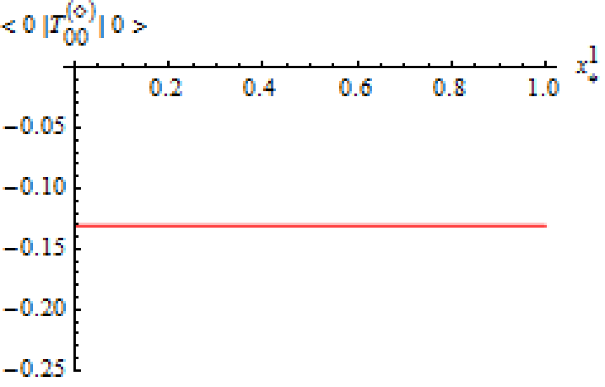
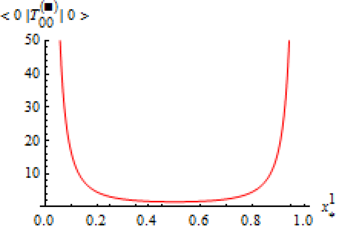
Figure 1: $d=1$: graphs of $\langle 0|\widehat{T}^{(\lozenge)}_{00}|0\rangle_{ren}$ and $\langle 0|\widehat{T}^{(\blacksquare)}_{00}|0\rangle_{ren}$ .

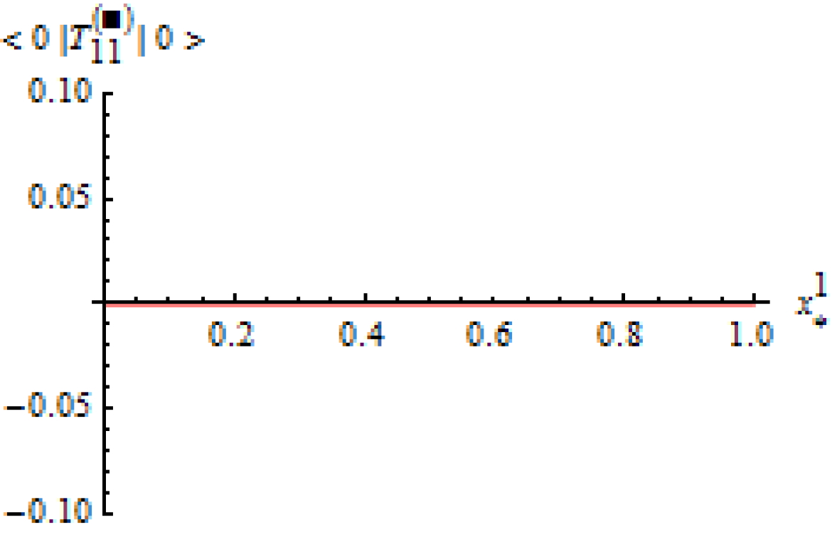
Figure 2: $d=1$: graphs of $\langle 0|\widehat{T}^{(\lozenge)}_{11}|0\rangle_{ren}$ and $\langle 0|\widehat{T}^{(\blacksquare)}_{11}|0\rangle_{ren}$ .

Let us comment briefly on the above graphs. Apart from $\langle 0|\widehat{T}^{(\blacksquare)}_{00}|0\rangle_{ren}$, it appears that all the other components of the renormalized stress-energy VEV are constants and $\langle 0|\widehat{T}^{(\blacksquare)}_{11}|0\rangle_{ren}$ is very small; indeed, our computations with $N=5$ ($T=1$, $\alpha=0.03$) ensure, for all ${\bf x}\equiv x_{\star}^{1}\in(0,1)$,

$$\begin{split}&\langle 0|\widehat{T}^{(\lozenge)}_{00}({\bf x})|0\rangle_{ren}=\langle 0|\widehat{T}^{(\lozenge)}_{11}({\bf x})|0\rangle_{ren}=-\,0.1308997\pm 8\cdot 10^{-7}~{},\\ &\hskip 85.35826pt|\langle 0|\widehat{T}^{(\blacksquare)}_{11}({\bf x})|0\rangle_{ren}|\leqslant 4\cdot 10^{-6}~{}.\end{split}$$ (4.6)

Concerning $\langle 0|\widehat{T}^{(\blacksquare)}_{00}({\bf x})|0\rangle_{ren}$ we have, for example,

$$\begin{split}&\langle 0|\widehat{T}^{(\blacksquare)}_{00}({\bf x})|0\rangle_{ren}=\left\{\!\begin{array}[]{ll}3.141593\pm 10^{-6}&\mbox{for $x_{\star}^{1}=1/4$}\\ 1.570796\pm 10^{-6}&\mbox{for $x_{\star}^{1}=1/2$}\end{array}\right.~{}.\end{split}$$ (4.7)

These results are in agreement with the exact calculations of subsection 6.6 of Part I, which gave the following outcomes (see Eq. (6.24) of the cited subsection with $a\equiv a_{1}=1$) ()

$$\begin{split}&\hskip 42.67912pt\langle 0|\widehat{T}^{(\lozenge)}_{00}({\bf x})|0\rangle_{ren}=\langle 0|\widehat{T}^{(\lozenge)}_{11}({\bf x})|0\rangle_{ren}=-{\pi\over 24}~{},\\ &\langle 0|\widehat{T}^{(\blacksquare)}_{00}({\bf x})|0\rangle_{ren}={\pi\over 2\sin^{2}(\pi x^{1})}~{},\qquad\langle 0|\widehat{T}^{(\blacksquare)}_{11}({\bf x})|0\rangle_{ren}=0~{}.\end{split}$$ (4.8)

Next, let us pass to the evaluation of

$$F_{ren}(0):=p^{ren}_{1}({\bf x})\Big{|}_{x^{1}=0}~{};$$ (4.9)

this is nominally the “pressure” on the boundary point $x^{1}=0$ but in fact coincides with the force on this point, due to the zero dimensionality of the boundary.

Let us consider the prescriptions (3.62); computing the derivative of the functions $D^{(>)}_{1/2}$, $D^{(<)}_{1/2}$ appearing therein with the choices $a_{1}=1$, $T=1$ and $N=5$, we obtain

$$F_{ren}(0)=0.1308997\pm 3\cdot 10^{-7}$$ (4.10)

(again, the error is obtained using the remainder estimates of subsection 3.8.2 with $\alpha=0.03$). The above result is in agreement with the exact expression $F_{ren}(0)={\pi\over 24}$ derived in subsection 6.6 of Part I (see Eq.s (6.24) (6.27), and set $a\equiv a_{1}=1$ therein). Finally, we consider the renormalized bulk energy $E^{ren}$; the series expansions (3.79) (3.80) derived in subsection 3.7 (with the previous choices of $a_{1},T,N$) allow us to infer

$$E^{ren}=-0.1308996938996\pm 3\cdot 10^{-13}$$ (4.11)

(where the error is obtained using the remainder estimates of subsection 3.7.2, again with $\alpha=0.03$). The result (4.11) agrees with the exact computation $E^{ren}=-{\pi\over 24}$ obtained in subsection 6.6 of Part I (see Eq. (6.26), and set $a\equiv a_{1}=1$ therein). Let us stress that our approximants by truncation, converge quite rapidly to the exact results; in order to exemplify this statement, we notice that, by slightly increasing the value of the truncation order $N$, we obtain a remarkable improvement of the error estimates. For example (using again the estimates of subsection 3.7.2 with $T=1$ and $\alpha=0.03$) the error $\pm 3\cdot 10^{-13}$ in Eq. (4.11) (for $N=5$) becomes $\pm 2\cdot 10^{-46}$ for $N=10$, $6\cdot 10^{-101}$ for $N=15$ and $4\cdot 10^{-177}$ for $N=20$.

4.2   Case $d=2$.

Let us now pass to the $2$-dimensional case:

$$d=2~{},\qquad\Omega=(0,a_{1})\times(0,a_{2})\quad(a_{1},a_{2}>0)~{}.$$ (4.12)

As in the previous subsection, we fix

$$a_{1}=1$$ (4.13)

and consider different values of $a_{2}$; let us repeat that the above choice does not imply a loss of generality, due to the scaling properties of subsection 3.9. Moreover, we present the final results in terms of the rescaled coordinates $x_{\star}^{1}:=x^{1}/a_{1}\equiv x^{1}$, $x_{\star}^{2}:=x^{2}/a_{2}\in(0,1)$, defined in Eq. (3.102) (). Again, the basic elements to compute the renormalized stress-energy VEV and the pressure are the Dirichlet functions $D_{s}^{(>)}$, $D_{s}^{(<)}$, along with their spatial derivatives, for which we use the truncated expansions (3.49-3.54) and the remainder bounds of Eq.s (3.49-3.54).

Needless to say, analogous considerations also hold for the renormalized bulk energy and for the integrated boundary forces (see subsections 3.7 and 3.8, respectively). Let us first consider the stress-energy VEV and the pressure; as examples, we compute these observables for the two configurations with

$$a_{2}=1\qquad\mbox{and}\qquad a_{2}=5~{}.$$ (4.14)

In these cases, for the parameter $T$ of the decomposition into $(>)$ and $(<)$ parts and for the truncation order $N$, we make the following choices:

$$\begin{split}&T=1~{},\quad N=7\qquad\mbox{for $a_{2}=1$}~{};\\ &T=1~{},\quad N=9\qquad\mbox{for $a_{2}=5$}~{}.\end{split}$$ (4.15)

The truncation errors in Eq.s (3.49-3.54) are evaluated making for the parameter $\alpha$ therein the choice ()

$$\alpha=0.04~{}.$$ (4.16)

The renormalized stress-energy VEV $\langle 0|\widehat{T}_{\mu\nu}|0\rangle_{ren}$ is obtained setting $u=0$ in Eq.s (3.55-3.58). Again, we separate the conformal and nonconformal parts, respectively indicated by the superscripts $(\lozenge)$ and $(\blacksquare)$; recall that Eq. (2.13) gives, in the two-dimensional case,

$$\xi_{2}=1/8~{}.$$ (4.17)

In the following we present the graphs for $\langle 0|\widehat{T}^{(\lozenge)}_{\mu\nu}|0\rangle_{ren}$ and $\langle 0|\widehat{T}^{(\blacksquare)}_{\mu\nu}|0\rangle_{ren}$ obtained from the previous truncated expansions; more precisely, Fig.s 3-5 and Fig.s 6-9 show, respectively, the results obtained for the configurations with $a_{2}=1$ and $a_{2}=5$ . In the cited figures we refer to the variables $x_{\star}^{i}:=x^{i}/a_{i}\in(0,1)$ and, keeping into account some obvious symmetry considerations (), we only show the graphs for

$$x_{\star}^{i}\in(0,1/2)\qquad\mbox{for $i\in\{1,2\}$}~{};$$ (4.18)

moreover, in the case of a square box with $a_{1}=a_{2}=1$ we do not report the graphs for the conformal and non-conformal parts of $\langle 0|\widehat{T}_{22}({\bf x})|0\rangle_{ren}$, since these are equal to the corresponding parts of $\langle 0|\widehat{T}_{11}({\bf x})|0\rangle_{ren}$.

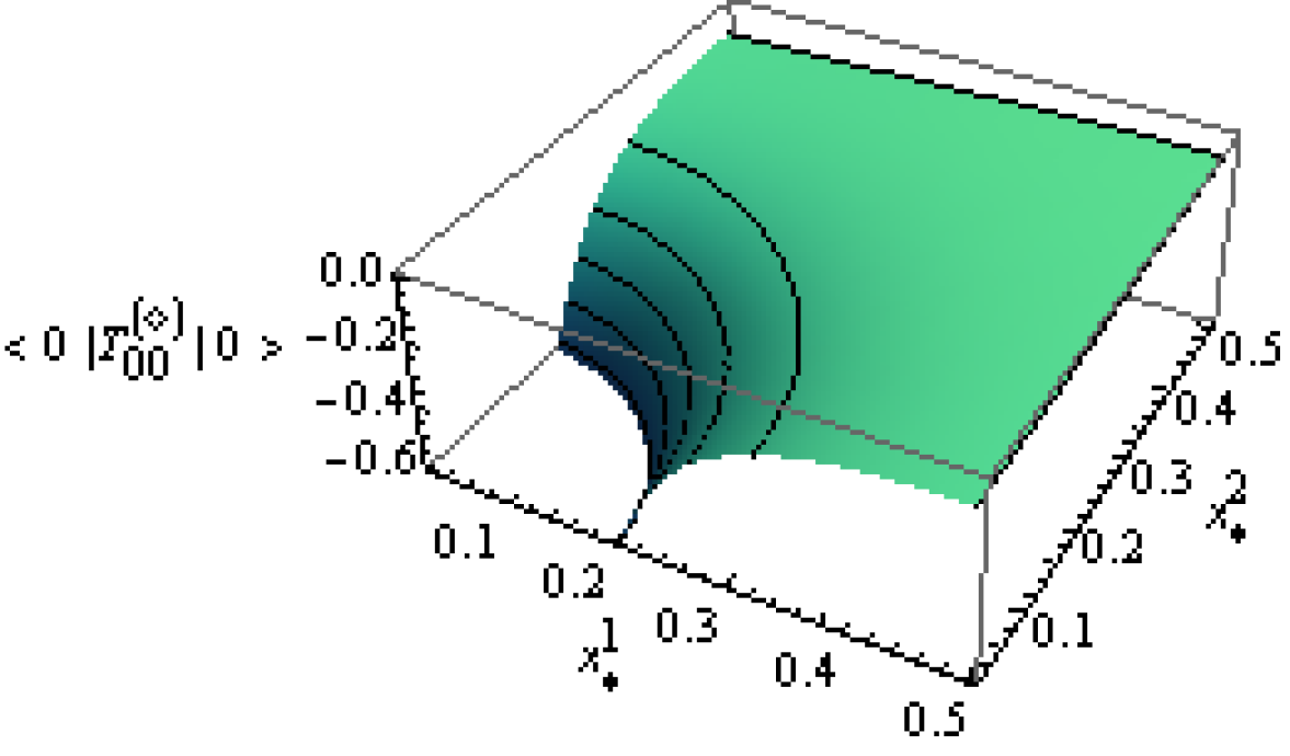
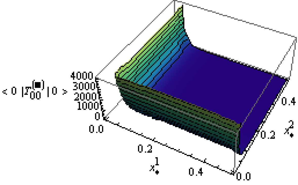
Figure 3: $d=2$: graphs of $\langle 0|\widehat{T}^{(\lozenge)}_{00}({\bf x})|0\rangle_{ren}$ and $\langle 0|\widehat{T}^{(\blacksquare)}_{00}({\bf x})|0\rangle_{ren}$ for $a_{2}=1$ .

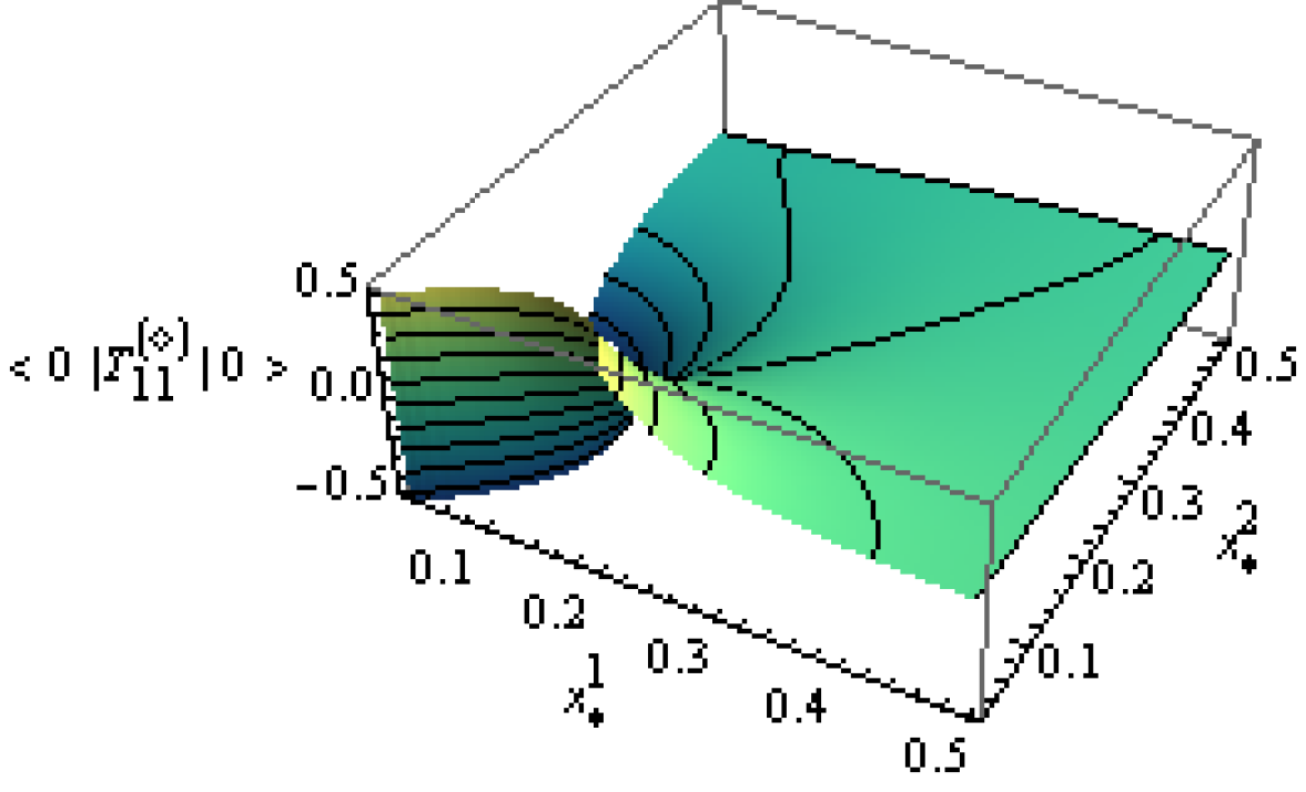
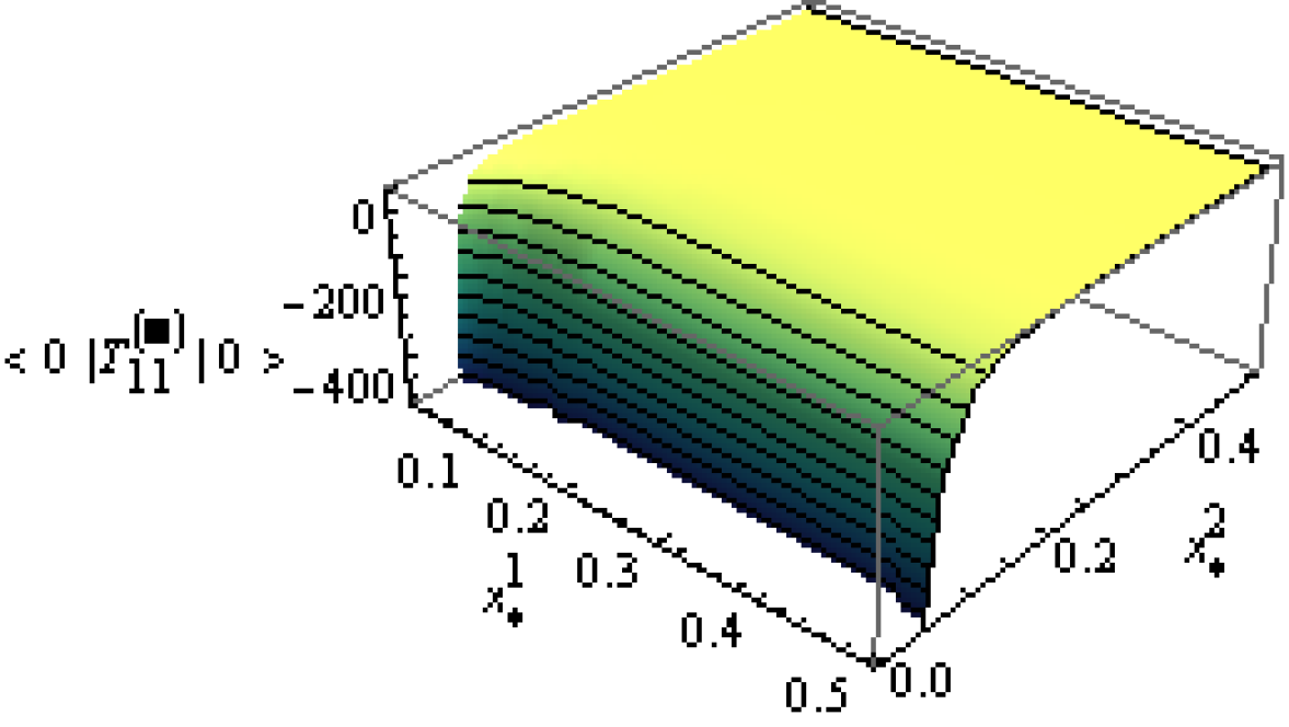
Figure 4: $d=2$: graphs of $\langle 0|\widehat{T}^{(\lozenge)}_{11}({\bf x})|0\rangle_{ren}$ and $\langle 0|\widehat{T}^{(\blacksquare)}_{11}({\bf x})|0\rangle_{ren}$ for $a_{2}=1$ .

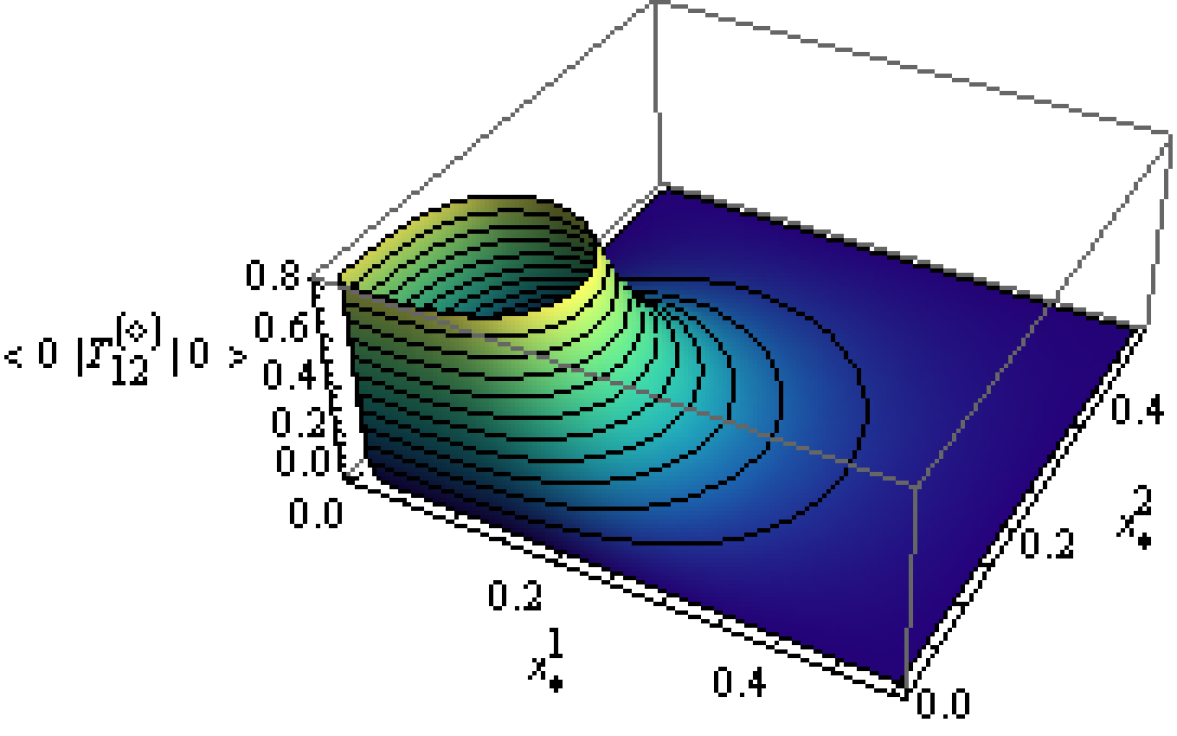
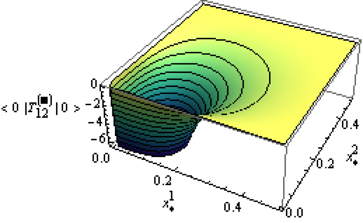
Figure 5: $d=2$: graphs of $\langle 0|\widehat{T}^{(\lozenge)}_{12}({\bf x})|0\rangle_{ren}$ and $\langle 0|\widehat{T}^{(\blacksquare)}_{12}({\bf x})|0\rangle_{ren}$ for $a_{2}=1$ .

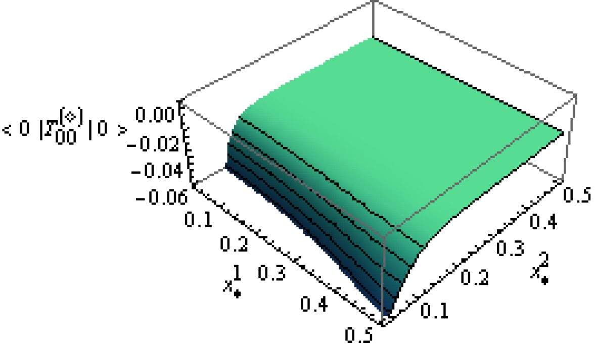
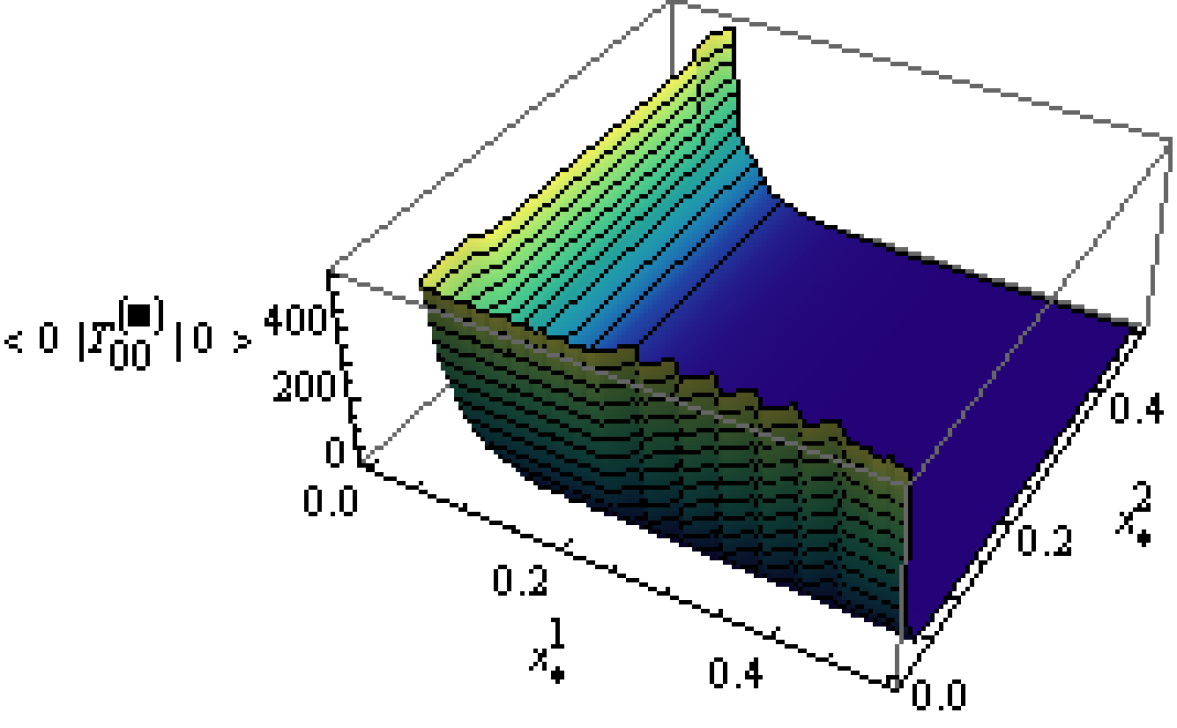
Figure 6: $d=2$: graphs of $\langle 0|\widehat{T}^{(\lozenge)}_{00}({\bf x})|0\rangle_{ren}$ and $\langle 0|\widehat{T}^{(\blacksquare)}_{00}({\bf x})|0\rangle_{ren}$ for $a_{2}=5$ .

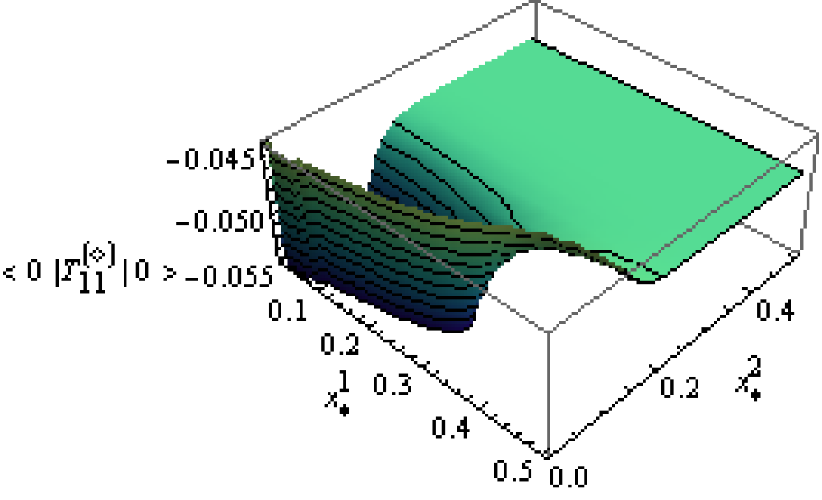
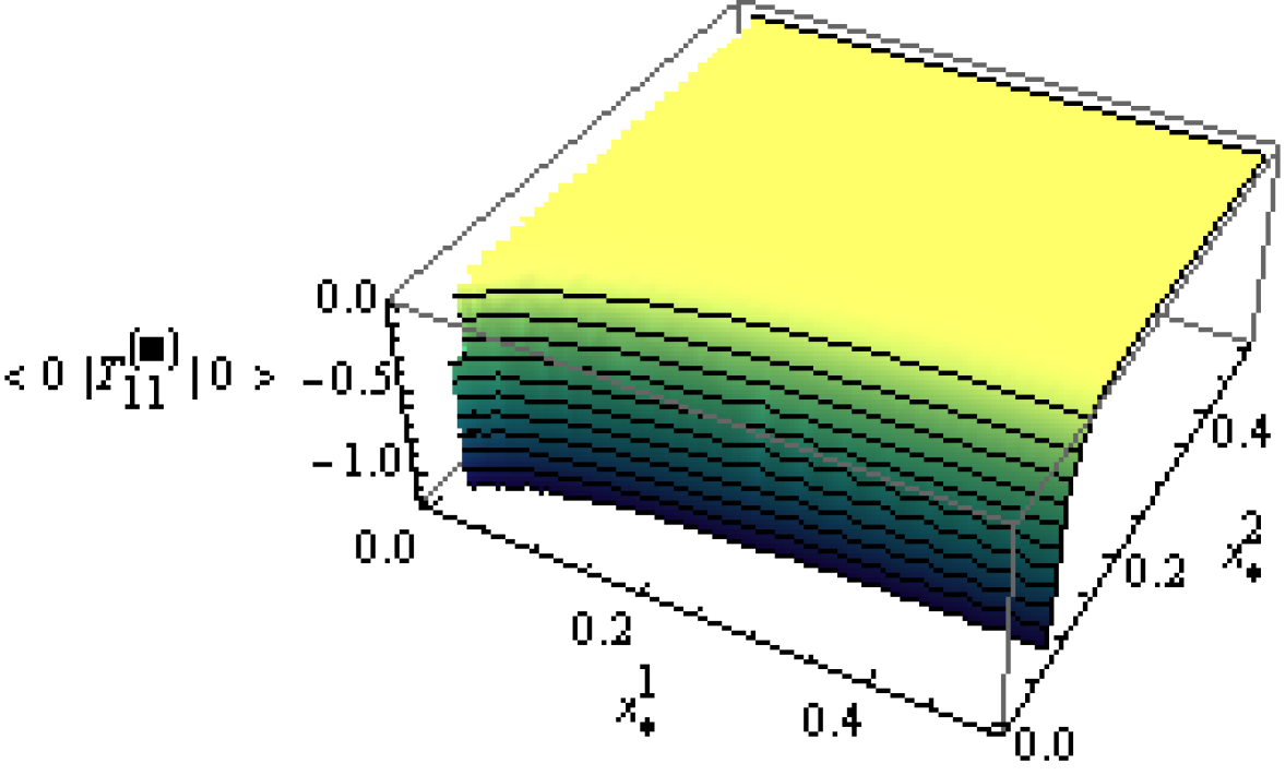
Figure 7: $d=2$: graphs of $\langle 0|\widehat{T}^{(\lozenge)}_{11}({\bf x})|0\rangle_{ren}$ and $\langle 0|\widehat{T}^{(\blacksquare)}_{11}({\bf x})|0\rangle_{ren}$ for $a_{2}=5$ .

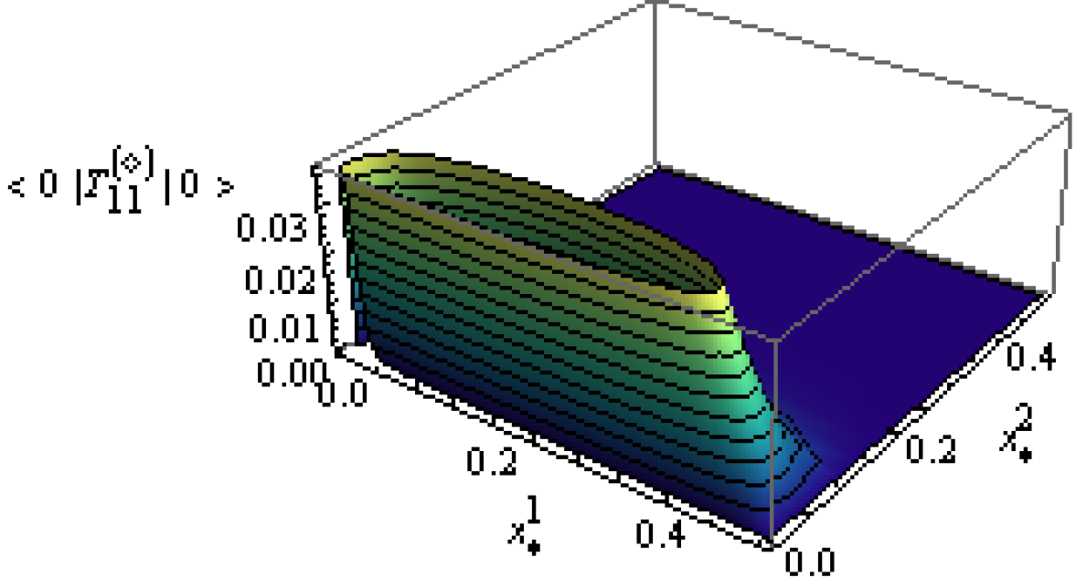
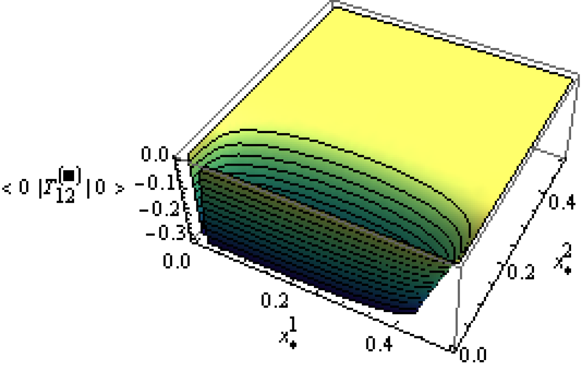
Figure 8: $d=2$: graphs of $\langle 0|\widehat{T}^{(\lozenge)}_{12}({\bf x})|0\rangle_{ren}$ and $\langle 0|\widehat{T}^{(\blacksquare)}_{12}({\bf x})|0\rangle_{ren}$ for $a_{2}=5$ .

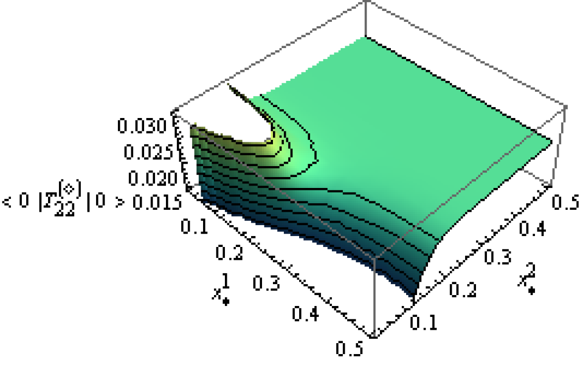
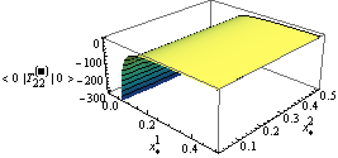
Figure 9: $d=2$: graphs of $\langle 0|\widehat{T}^{(\lozenge)}_{22}({\bf x})|0\rangle_{ren}$ and $\langle 0|\widehat{T}^{(\blacksquare)}_{22}({\bf x})|0\rangle_{ren}$ for $a_{2}=5$ .

Concerning the error estimates, for $\mu,\nu\in\{0,1,2\}$ and $\bullet\in\{\lozenge,\blacksquare\}$, let us introduce the following notation:

$$\mathcal{E}_{\mu\nu}^{(\bullet)}:=\begin{array}[]{c}\mbox{remainder corresponding to our approximation}\\ \mbox{by truncation of $\langle 0|\widehat{T}_{\mu\nu}^{(\bullet)}|0\rangle_{ren}$\,.}\end{array}$$ (4.19)

For $a_{2}=1$, our choice $N=7$ ($T=1$, $\alpha=0.04$) yields the uniform bounds

$$\begin{split}&\hskip 48.36958pt|\mathcal{E}_{00}^{(\lozenge)}|\leqslant 2\cdot 10^{-12}~{},\qquad|\mathcal{E}_{00}^{(\blacksquare)}|\leqslant 2\cdot 10^{-11}~{};\\ &|\mathcal{E}_{ij}^{(\lozenge)}|\leqslant 6\cdot 10^{-12}~{},\qquad|\mathcal{E}_{ij}^{(\blacksquare)}|\leqslant 3\cdot 10^{-11}\qquad\mbox{for $i,j\in\{1,2\}$}~{}.\end{split}$$ (4.20)

For $a_{2}=5$, our choice $N=9$ ($T=1$, $\alpha=0.04$) ensures

$$\begin{split}&\hskip 51.21504pt|\mathcal{E}_{00}^{(\lozenge)}|\leqslant 5\cdot 10^{-12}~{},\qquad|\mathcal{E}_{00}^{(\blacksquare)}|\leqslant 4\cdot 10^{-11}~{};\\ &|\mathcal{E}_{ij}^{(\lozenge)}|\leqslant 2\cdot 10^{-11}~{},\qquad|\mathcal{E}_{ij}^{(\blacksquare)}|\leqslant 8\cdot 10^{-11}\qquad\mbox{for $i,j\in\{1,2\}$}~{}.\end{split}$$ (4.21)

Now, let us evaluate the pressure $p_{i}^{ren}({\bf x})$ at points ${\bf x}$ of one side; as in the construction of the general theory we consider, as an example, the points ${\bf x}\equiv(0,x^{2})$ in the interior of the side $\pi_{1,0}$, making reference to the prescription (3.62).

Fig. 10 shows the graphs obtained for $p_{1}^{ren}({\bf x})$ as a function of $x^{2}_{\star}:=x^{2}/a_{2}$ (again, choosing $T=1$ and truncating the related expansions to order $N=7$, for $a_{2}=1$, and $N=9$, for $a_{2}=5$).

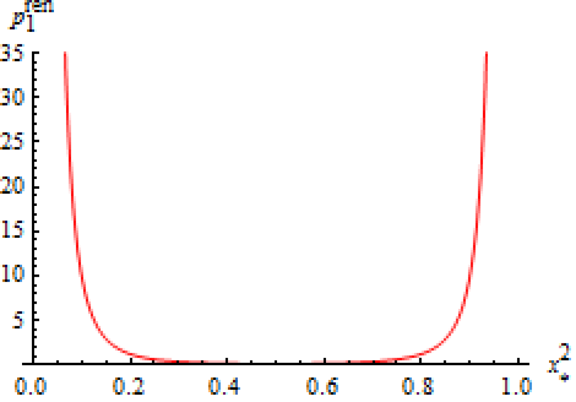
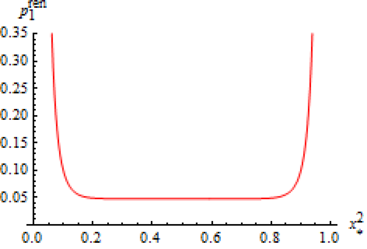
Figure 10: $d=2$: graphs of $p_{1}^{ren}$ for $a_{2}=1$ (left) and $a_{2}=5$ (right).

As for the error, indicating with $\epsilon_{1}$ the remainder associated to our approximation by truncation of $p_{1}^{ren}$, we obtain the following uniform estimates (setting $\alpha=0.04$):

$$\begin{split}&|\epsilon_{1}|\leqslant 2\cdot 10^{-12}\qquad\mbox{for $a_{2}=1$}~{};\\ &|\epsilon_{1}|\leqslant 5\cdot 10^{-12}\qquad\mbox{for $a_{2}=5$}~{}.\end{split}$$ (4.22)

Before moving on, let us briefly comment on the behaviour of the renormalized pressure $p_{1}^{ren}$ near the edge ${\bf x}=\textbf{0}$. Indeed, specializing to the present $d=2$ case the considerations of paragraph 3.6.2 one can prove that, for all $a_{2}>0$,

$$p_{1}^{ren}({\bf x})={1\over 32\pi(x^{2})^{3}}+O((x^{2})^{2})\qquad\mbox{for ${\bf x}=(0,x^{2})$ and $x^{2}\to 0^{+}$}~{}.$$ (4.23)

Now, let us pass to the computation of the bulk energy and of the integrated force. For each one of these two observables we consider several configurations, corresponding to different values of $a_{2}$; for any one of these values, we consider the decomposition into $(>)$ and $(<)$ parts, and choose the truncation order $N$ of the related expansions so as to obtain error estimates all of approximatively the same order of magnitude, fixing again

$$\alpha=0.04~{}.$$ (4.24)

In order to obtain the renormalized bulk energy $E^{ren}$, we first consider its regularized version (3.78), along with the series expansions (3.79) (3.80), giving the analytic continuations of the functions $E^{u,(>)}$ and $E^{u,(<)}$, respectively. Due to the considerations of subsection 3.7, we can simply put $u=0$ in these expansions, since no singularity arises there; next, we truncate the corresponding series at a suitable order $N$ (see the comments above) and use the remainder estimates (3.85) (3.87).

In this way we obtain, for example, the following results: for $a_{1}=1$ (and with the choice $T=1$, as usual)

$$\begin{array}[]{lll}E^{ren}=-\,1.73691776\pm 4\cdot 10^{-8}&\mbox{for $a_{2}=0.1$}&(N=40)~{};\\ E^{ren}=+\,0.03524178\pm 3\cdot 10^{-8}&\mbox{for $a_{2}=0.5$}&(N=8)~{};\\ E^{ren}=+\,0.04104060\pm 9\cdot 10^{-8}&\mbox{for $a_{2}=1$}&(N=4)~{};\\ E^{ren}=-\,0.05412096\pm 2\cdot 10^{-8}&\mbox{for $a_{2}=5$}&(N=7)~{};\\ E^{ren}=-\,0.17369178\pm 1\cdot 10^{-8}&\mbox{for $a_{2}=10$}&(N=15)~{}.\end{array}$$ (4.25)

Again for $a_{1}=1$, one can plot the renormalized bulk energy $E^{ren}$ as a function of $a_{2}$; the graph in Fig. 11 has been obtained using the truncation order $N=50$ (with $T=1$; with the choices made for the parameters $N,T,a_{1}$, we know that the remainder is smaller than $2\cdot 10^{-3}$ for $a_{2}\in[0.05,10)$).

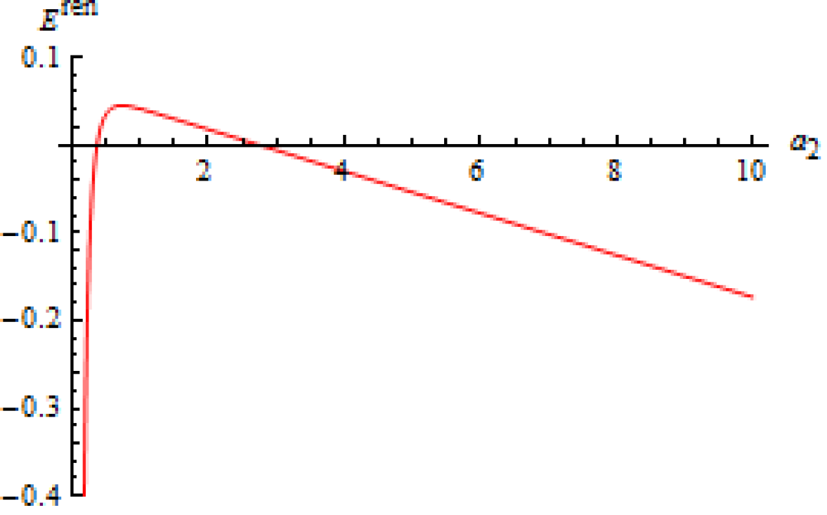
Figure 11: $d=2$: graph of $E^{ren}$ as function of $a_{2}$ .

Let us discuss some facts regarding the function $a_{2}\mapsto E^{ren}(a_{2})$, which can be read from the graph in Fig. 11 (the results reported hereafter are obtained using standard numerical methods, implemented in $\tt{Mathematica}$) ().

i) There is only one point of maximum $a_{2}^{\max}$; our approximation by truncation at order $N=50$ gives

$$\begin{split}&\hskip 19.91684pta_{2}^{\max}=0.72719110\pm 10^{-8}~{},\\ &E^{ren}(a_{2}^{\max})=0.04472675\pm 10^{-8}~{}.\end{split}$$ (4.26)

ii) $E^{ren}$ vanishes for two values $\bar{a}_{2}^{(1)}<\bar{a}_{2}^{(2)}$ of $a_{2}$; these are found to be

$$\begin{split}&\hskip 2.84544pt\bar{a}_{2}^{(1)}=0.36538151\pm 10^{-8}~{},\\ &\bar{a}_{2}^{(2)}=2.73686534\pm 10^{-8}~{}.\end{split}$$ (4.27)

$E^{ren}$ is positive for $\bar{a}_{2}^{(1)}\!<a_{2}<\bar{a}_{2}^{(2)}$ and negative elsewhere. This feature was also pointed out in [22]; therein it is stated that $\bar{a}_{2}^{(2)}=(\bar{a}_{2}^{(1)})^{-1}$, a relation (approximately) verified by the numerical values in Eq. (4.27).

iii) For $a_{2}\to 0^{+}$, $E^{ren}$ has the asymptotic behaviour

$$E^{ren}(a_{2})={e_{0}\over(a_{2})^{2}}\;\Big{(}1+O(a_{2})\Big{)}\quad\mbox{with}\quad e_{0}=-0.02391\pm 10^{-5}~{}.$$ (4.28)

iv) There are indications that $E^{ren}$ approaches an asymptote for $a_{2}\to+\infty$; taking into account values of the abscissa up to $a_{2}=100$, we find that this asymptote is the straight line

$$\begin{split}y=m_{E}\,a_{2}+q_{E}\qquad\mbox{with}\quad\left\{\!\begin{array}[]{l}m_{E}=-\,0.02391416\pm 10^{-8}\\ q_{E}=+\,0.06544985\pm 10^{-8}\end{array}\right.\,.\end{split}$$ (4.29)

Finally, let discuss the renormalized total force $\mathfrak{F}_{1,0}^{ren}$ acting on the side $\pi_{1,0}$; following the analysis of subsection 3.8, we consider the expression (3.96) and represent the functions $\mathfrak{F}_{1,0}^{u,(>)}$, $\mathfrak{F}_{1,0}^{u,(<)}$ appearing therein using the series expansions (3.92) (3.93). $\mathfrak{F}_{1,0}^{ren}$ is obtained setting $u=0$ in these series expansions; for the actual calculation, these can be truncated at a fixed, sufficiently large order $N$ using the remainder estimates (3.98) (3.100).

In this way we obtain, for example, the following results: for $a_{1}=1$ (and with the choice $T=1$, as usual)

$$\begin{array}[]{lll}\mathfrak{F}_{1,0}^{ren}=+\,2.3914162\pm 4\cdot 10^{-7}&\mbox{for $a_{2}=0.1$}&(N=50)~{};\\ \mathfrak{F}_{1,0}^{ren}=+\,0.0956400\pm 2\cdot 10^{-7}&\mbox{for $a_{2}=0.5$}&(N=9)~{};\\ \mathfrak{F}_{1,0}^{ren}=+\,0.020520\pm 6\cdot 10^{-6}&\mbox{for $a_{2}=1$}&(N=4)~{};\\ \mathfrak{F}_{1,0}^{ren}=-\,0.173692\pm 4\cdot 10^{-6}&\mbox{for $a_{2}=5$}&(N=7)~{};\\ \mathfrak{F}_{1,0}^{ren}=-\,0.412833\pm 3\cdot 10^{-6}&\mbox{for $a_{2}=10$}&(N=15)~{}.\end{array}$$ (4.30)

Again for $a_{1}=1$, one can plot the renormalized force $\mathfrak{F}_{1,0}^{ren}$ as a function of $a_{2}$; the graph in Fig. 12 has been obtained using the truncation order $N=60$ (with $T=1$; with the choices made for the parameters $N,T,a_{1}$, we know that the remainder is smaller than $2\cdot 10^{-3}$ for $a_{2}\in[0.07,10)$).

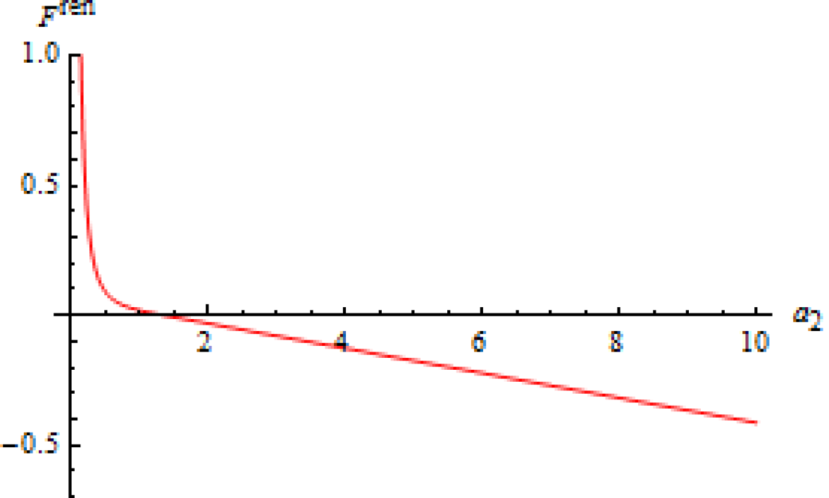
Figure 12: $d=2$: graph of $\mathfrak{F}_{1,0}^{ren}$ as function of $a_{2}$ .

In the following we briefly discuss a number of facts concerning the function $a_{2}\mapsto\mathfrak{F}_{1,0}^{ren}(a_{2})$, which appear in the above graph.

i) The function under analysis is strictly decreasing for $a_{2}\in(0,+\infty)$ .

ii) There is only one value of $a_{2}$, which we indicate with $\bar{a}_{2}$, where $\mathfrak{F}_{1,0}^{ren}$ vanishes; our approximation by truncation at order $N=60$ allows us to infer

$$\bar{a}_{2}=1.3751543\pm 10^{-7}~{}.$$ (4.31)

iii) For $a_{2}\to 0^{+}$, $\mathfrak{F}_{1,0}^{ren}$ has the asymptotic behaviour

$$\mathfrak{F}_{1,0}^{ren}(a_{2})={f_{0}\over(a_{2})^{2}}\;\Big{(}1+O(a_{2})\Big{)}\quad\mbox{with}\quad f_{0}=0.02391\pm 10^{-5}~{}.$$ (4.32)

iv) It appears that $\mathfrak{F}_{1,0}^{ren}$ approaches an asymptote for $a_{2}\to+\infty$; considering again values of the abscissa up to $a_{2}=100$, the equation of this asymptote is found to be

$$\begin{split}y=m\,a_{2}+q\qquad\mbox{with}\quad\left\{\!\begin{array}[]{l}m=-\,0.0478283\pm 10^{-7}\\ q=+\,0.0654498\pm 10^{-7}\end{array}\right.\,.\end{split}$$ (4.33)

Let us mention that, in agreement with the general considerations of subsection 4.4 in Part I, the above results for the renormalized total force on the side $\pi_{1,0}$ of the box could be equivalently derived by differentiating the renormalized total energy $E^{ren}$ with respect to the lenght $a_{2}$ of the edge of the box perpendicular to $\pi_{1,0}$. To conclude, let us compare the previous results about $E^{ren},\mathfrak{F}_{1,0}^{ren}$ with the calculations of Bordag et al. [5]. The authors of [5] derive (both by Abel-Plana formula and by zeta regularization) series expansions different from ours for the renormalized bulk energy and for the force on one side; besides, they give no remainder estimates for these expansions ().

The numerical values of $E^{ren},\mathfrak{F}_{1,0}^{ren}$ given by our previous analysis are in good agreement with those arising from the expansions in [5], a fact strongly indicating the equivalence between our approach and [5]. Let us also mention that the results of [5] about $E^{ren}$ or $\mathfrak{F}_{1,0}^{ren}$ are equivalent to the ones of [3, 11, 16]. Acknowledgments. This work was partly supported by INdAM, INFN and by MIUR, PRIN 2010 Research Project “Geometric and analytic theory of Hamiltonian systems in finite and infinite dimensions”.

Appendix A Appendix. Absolute convergence and remainder bounds for the series of subsections 3.3.

Let us consider the general framework of the subsections mentioned in the title. Note that the representation (3.30) for the function $D_{s}^{(>)}({\bf x},{\bf y})$ contains the series

$$\sum_{{\bf n}\in{\bf N}^{d}}\omega_{\bf n}^{-2s}\,\Gamma(s,\omega_{\bf n}^{2}\,T)\;C_{\bf n}({\bf x},{\bf y})~{}.$$ (A.1)

On the other hand, in the expansion (3.36) for $D_{s}^{(<)}({\bf x},{\bf y})$ there appears a series over ${\bf h}\!\in\!{\bf Z}^{d}$ and ${\bf l}\!\in\!\{1,2\}^{d}$ , that we have reexpressed in the equivalent form (3.39). We pointed out in paragraph 3.3.2 that the terms in this series with $b_{{\bf h}{\bf l}}({\bf x},{\bf y})=0$ become singular at $s={d/2}$ ; these have either $|{\bf h}|=0$ or $|{\bf h}|=1$ (see Eq. (3.22)) and, after removing all terms with $|{\bf h}|=0,1$ we are left with the series

$$\sum_{\begin{subarray}{c}{\bf h}\in{\bf Z}^{d},\,|{\bf h}|>1\\ {\bf l}\in\{1,2\}^{d}\end{subarray}}\delta_{\bf l}\;{\mathcal{P}}_{s-{d\over 2}}\!\left({b_{{\bf h}{\bf l}}({\bf x},{\bf y})\over T}\right)\,.$$ (A.2)

Note that the absolute convergence of the series (A.2) is equivalent to the absolute convergence of the series in the second line of Eq. (3.39).

In the next subsections we prove the convergence of the series (A.1) (A.2) for all $s\in{\bf C}$ , deriving as well remainder estimates for both of them; the statements in Eq.s (3.30) (3.50) (related to $D_{s}^{(>)}({\bf x},{\bf y})$) and in Eq.s (3.36) (3.53) (related to $D_{s}^{(<)}({\bf x},{\bf y})$) follow easily from these results.

The arguments presented in this appendix can be easily generalized to derive the analogous conclusions for the series in Eq.s (3.31) (3.51) and (3.37) (3.54) related to the derivatives $\partial_{zw}D_{s}^{(>)}({\bf x},{\bf y})$ and $\partial_{zw}D_{s}^{(<)}({\bf x},{\bf y})$; we will briefly return on this topic in the sequel (see subsections A.2 and A.3).

In the final subsection of this appendix we also derive the asymptotic (3.47) for the function $H^{(d)}_{N}$ in our remainder estimates. Before proceeding, let us recall the following definitions (see Eq. (3.45)):

$$a:=\min_{i\in\{1,...,d\}}\{a_{i}\}\,,\;\;A:=\max_{i\in\{1,...,d\}}\{a_{i}\}\,,\quad|{\bf z}|^{2}:=\sum_{i=1}^{d}z_{i}^{2}\;\;\mbox{for ${\bf z}={\bf n}\!\in\!{\bf N}^{d}$ or ${\bf z}={\bf h}\!\in\!{\bf Z}^{d}$}\,.$$

A.1   Preliminary estimates.

First of all, let us consider the upper incomplete gamma function (see Eq. (3.29))

$$\Gamma(s,z):=\int_{z}^{+\infty}\!\!dw\;e^{-w}\,w^{s-1}\qquad(s\in{\bf C},\,z\in(0,+\infty))$$

and note that the above definition implies the following:

$$|\Gamma(s,z_{2})|\leqslant\Gamma(\Re s,z_{1})\qquad\mbox{for all $s\!\in\!{\bf C}$, $z_{1},z_{2}\!\in\!(0,+\infty)$ with $0\!<\!z_{1}\!\leqslant\!z_{2}$}~{};$$ (A.3)

$$|\Gamma(s,z)|\leqslant(1\!-\!\alpha)^{-\Re s}e^{-\alpha z}\,\Gamma(\Re s,(1\!-\!\alpha)z)\quad\mbox{for all $s\!\in\!{\bf C}$, $z\!\in\!(0,+\infty)$, $\alpha\!\in\!(0,1)$}\,.\!$$ (A.4)

Hereafter we are going to prove that

$$\begin{split}&\hskip 59.75095pt\sum_{{\bf h}\in{\bf Z}^{d},\,|{\bf h}|>N}|{\bf h}|^{\rho}\,|\Gamma(s,\beta|{\bf h}|^{2})|\leqslant H^{(d)}_{N}(\alpha,\beta;\Re s,\rho)\\ &\begin{array}[]{c}\mbox{for all $s\in{\bf C}$, $N,\rho\in{\bf R}$, $\beta\in(0,+\infty)$, $\alpha\in(0,1)$ such that}\\ \mbox{either $\rho\leqslant 0$ and $N>2\sqrt{d}$}\quad\mbox{or}\quad\mbox{$\rho>0$ and $\displaystyle{N>2\sqrt{d}+\sqrt{\rho\over 2\alpha\beta}}$}~{},\end{array}\end{split}$$ (A.5)

where $H^{(d)}_{N}$ is defined according to Eq. (3.46), i.e. (for $\sigma\in{\bf R}$),

$$H^{(d)}_{N}(\alpha,\beta;\sigma,\rho):=$$

$${\pi^{d/2}\over(1\!-\!\alpha)^{\sigma}(\alpha\,\beta)^{{d+\rho\over 2}}\,\Gamma({d\over 2})}\left({N\!-\!\sqrt{d}\over N\!-\!2\sqrt{d}}\right)^{\!\!\!d-1}\!\Gamma(\sigma,(1\!-\!\alpha)\beta N^{2})\;\Gamma\!\left({d\!+\!\rho\over 2}\,;\alpha\,\beta(N\!-\!2\sqrt{d})^{2}\right)\,.$$

In the sequel we always assume $s\!\in\!{\bf C}$, $\rho\!\in\!{\bf R}$, $N\!\in\!(2\sqrt{d},+\infty)$, $\beta\!\in\!(0,+\infty)$, $\alpha\!\in\!(0,1)$.

In order to derive the estimate (A.5) we first point out that, due to Eq.s (A.3) (A.4), there holds

$$\begin{split}&|\Gamma(s,\beta|{\bf h}|^{2})|\leqslant(1\!-\!\alpha)^{-\Re s}\,e^{-\alpha\beta|{\bf h}|^{2}}\,\Gamma(\Re s,(1\!-\!\alpha)\beta N^{2})\\ &\hskip 62.59596pt\mbox{for all ${\bf h}\!\in\!{\bf Z}^{d}$ with $|{\bf h}|\!>\!N$}~{};\end{split}$$ (A.6)

this in turn implies

$$\sum_{{\bf h}\in{\bf Z}^{d},\,|{\bf h}|>N}|{\bf h}|^{\rho}\,|\Gamma(s,\beta|{\bf h}|^{2})|\!\leqslant(1\!-\!\alpha)^{-\Re s}\,\Gamma(\Re s,(1\!-\!\alpha)\beta N^{2})\!\!\sum_{{\bf h}\in{\bf Z}^{d},\,|{\bf h}|>N}|{\bf h}|^{\rho}\,e^{-\alpha\beta|{\bf h}|^{2}}~{}.$$ (A.7)

To proceed, let us note that, for any non-increasing function $F:[N\!-\!2\sqrt{d},+\infty)\!\to\![0,+\infty)$, there holds the following estimate (see, e.g., [28], p. 691):

$$\sum_{{\bf h}\in{\bf Z}^{d},\,|{\bf h}|>N}F(|{\bf h}|)\leqslant{2\pi^{d/2}\over\Gamma({d\over 2})}\int_{N-2\sqrt{d}}^{+\infty}d\tau\;(\tau\!+\!\sqrt{d})^{d-1}F(\tau)~{};$$ (A.8)

noting that $\tau\!+\!\sqrt{d}=\Big{(}1\!+\!{\sqrt{d}\over\tau}\Big{)}\tau\leqslant\Big{(}{N\!-\!\sqrt{d}\over N\!-\!2\sqrt{d}}\Big{)}\tau$ (for $\tau\!>\!N\!-\!2\sqrt{d}>0$), the above inequality yields

$$\sum_{{\bf h}\in{\bf Z}^{d},\,|{\bf h}|>N}F(|{\bf h}|)\leqslant{2\pi^{d/2}\over\Gamma({d\over 2})}\left({N\!-\!\sqrt{d}\over N\!-\!2\sqrt{d}}\right)^{\!\!\!d-1}\!\int_{N-2\sqrt{d}}^{+\infty}d\tau\;\tau^{d-1}F(\tau)~{}.$$ (A.9)

We want to employ the above bound to estimate the sum in the right-hand side of Eq. (A.7); this case involves the function

$$F(\tau)=\tau^{\rho}\,e^{-\alpha\beta\,\tau^{2}}~{},$$ (A.10)

which is decreasing on $[N\!-\!2\sqrt{d},+\infty)$ for

$$\mbox{either $\rho\leqslant 0$ and $N\!>2\sqrt{d}$ (as before)}\quad\mbox{or}\quad\mbox{$\rho>0$ and $\displaystyle{N\!>2\sqrt{d}+\!\sqrt{\rho\over 2\alpha\beta}}$}\,.$$ (A.11)

In each one of the above two situations, making the change of variable $v:=\alpha\,\beta\,\tau^{2}\in[\alpha\,\beta(N\!-\!2\sqrt{d})^{2},+\infty)$ and recalling the definition (3.29) of the upper incomplete gamma function, we easily obtain

$$\int_{N-2\sqrt{d}}^{+\infty}d\tau\;\tau^{d+\rho-1}\,e^{-\alpha\beta\,\tau^{2}}={1\over 2(\alpha\,\beta)^{{d+\rho\over 2}}}\;\Gamma\!\left({d\!+\!\rho\over 2}\,;\alpha\,\beta(N\!-\!2\sqrt{d})^{2}\right)\,,$$ (A.12)

which, along with Eq.s (A.7) (A.9) and (A.10), proves Eq. (A.5). In passing we point out that Eq. (A.5) implies the analogous estimate ()

$$\begin{split}&\hskip 51.21504pt\sum_{{\bf n}\in{\bf N}^{d},\,|{\bf n}|>N}|{\bf n}|^{\rho}\,|\Gamma(s,\beta|{\bf n}|^{2})|\leqslant{1\over 2^{d}}\;H^{(d)}_{N}(\alpha,\beta;\Re s,\rho)\\ &\begin{array}[]{c}\mbox{for all $s\in{\bf C}$, $N,\rho\in{\bf R}$, $\beta\in(0,+\infty)$, $\alpha\in(0,1)$ such that}\\ \mbox{either $\rho\leqslant 0$ and $N>2\sqrt{d}$}\quad\mbox{or}\quad\mbox{$\rho>0$ and $\displaystyle{N>2\sqrt{d}+\sqrt{\rho\over 2\alpha\beta}}$}~{}.\end{array}\end{split}$$ (A.13)

A.2   The series (A.1); connections with the expansions (3.30) (3.31) for $D^{(>)}_{s}$ and its derivatives.

For $s\!\in\!{\bf C}$ and $N\!\in\!(0,+\infty)$, let us define

$${\mathcal{R}}^{(>)}_{s,N}({\bf x},{\bf y}):=\sum_{{\bf n}\in{\bf N}^{d},\,|{\bf n}|>N}\Big{|}\omega_{\bf n}^{-2s}\,\Gamma(s,\omega_{\bf n}^{2}\,T)\;C_{\bf n}({\bf x},{\bf y})\Big{|}~{};$$ (A.14)

of course, the series (A.1) is absolutely convergent if and only if ${\mathcal{R}}^{(>)}_{s,N}({\bf x},{\bf y})<+\infty$ for some $N$ . The rest of this subsection will be mostly dedicated to evaluating ${\mathcal{R}}^{(>)}_{s,N}({\bf x},{\bf y})$ .

First of all, note that from the definitions (3.11) of $C_{\bf n},\omega_{\bf n}^{2}$ and (3.45) of $a,A$ it easily follows, for all ${\bf n}\in{\bf N}^{d}$,

$$|C_{\bf n}({\bf x},{\bf y})|\leqslant 1~{},$$ (A.15)

$${\pi^{2}\over A^{2}}\,|{\bf n}|^{2}\leqslant\omega_{\bf n}^{2}\leqslant{\pi^{2}\over a^{2}}\,|{\bf n}|^{2}~{}.$$ (A.16)

Using Eq. (A.16) we infer, for all $s\in{\bf C}$, ${\bf n}\in{\bf N}^{d}$,

$$|\omega_{\bf n}^{-2s}|\leqslant{\max(a^{2\Re s},A^{2\Re s})\over\pi^{2\Re s}}\;|{\bf n}|^{-2\Re s}~{},\qquad|\Gamma(s,\omega_{\bf n}^{2}\,T)|\leqslant\Gamma\!\left(\Re s,{\pi^{2}\,T\over A^{2}}\,|{\bf n}|^{2}\right)$$ (A.17)

(to deduce the second inequality we also employ Eq. (A.3)). Returning to the definition (A.14), we obtain

$${\mathcal{R}}^{(>)}_{s,N}({\bf x},{\bf y})\leqslant{{\max(a^{2\Re s},A^{2\Re s})}\,\over\,\pi^{2\Re s}}\sum_{{\bf n}\in{\bf N}^{d},\,|{\bf n}|>N}|{\bf n}|^{-2\Re s}\,\Gamma\!\left(\Re s,{\pi^{2}\,T\over A^{2}}\,|{\bf n}|^{2}\right)\,,$$ (A.18)

and using the estimate (A.13) we conclude the following, for any $\alpha\in(0,1)$:

$$\begin{split}&\hskip 34.14322pt{\mathcal{R}}^{(>)}_{s,N}({\bf x},{\bf y})\leqslant{\max(a^{2\Re s},A^{2\Re s})\over 2^{d}\,\pi^{2\Re s}}\;H^{(d)}_{N}\!\left(\!\alpha,{\pi^{2}\,T\over A^{2}}\,;\Re s,-2\Re s\!\right)\\ &\mbox{for either \quad$\Re s\geqslant 0$, $N>2\sqrt{d}$}\quad\mbox{or}\quad\mbox{$\Re s<0$, $\displaystyle{N>2\sqrt{d}+{A\over\pi}\sqrt{|\Re s|\over\alpha T}}$}~{}.\end{split}$$ (A.19)

As noted before, the finiteness of ${\mathcal{R}}^{(>)}_{s,N}({\bf x},{\bf y})$ proves the absolute convergence for all $s\in{\bf C}$ of the series (A.1), contained in Eq. (3.30) for $D^{(>)}_{s}({\bf x},{\bf y})$; the bound (3.50) for the remainder $R^{(>)}_{s,N}({\bf x},{\bf y})$ of Eq. (3.49) follows straightforwardly from Eq. (A.19) since we have

$$|R^{(>)}_{s,N}({\bf x},{\bf y})|\leqslant{2^{d}\over a_{1}...a_{d}\,|\Gamma(s)|}\;{\mathcal{R}}^{(>)}_{s,N}({\bf x},{\bf y})~{}.$$ (A.20)

Let us mention that the series in Eq. (3.31) for $\partial_{zw}D^{(>)}_{s}$ can be discussed similarly; in place of ${\mathcal{R}}^{(>)}_{s,N}({\bf x},{\bf y})$, we use the quantity

$$\phantom{{\mathcal{R}}^{>}}{}_{(z,w)}{\mathcal{R}}^{(>)}_{s,N}({\bf x},{\bf y}):=\sum_{{\bf n}\in{\bf N}^{d},\,|{\bf n}|>N}\Big{|}\omega_{\bf n}^{-2s}\,\Gamma(s,\omega_{\bf n}^{2}\,T)\;\partial_{zw}C_{\bf n}({\bf x},{\bf y})\Big{|}$$ (A.21)

and we estimate it similarly to what we did with ${\mathcal{R}}^{(>)}_{s,N}({\bf x},{\bf y})$, noting that

$$|\partial_{zw}C_{\bf n}({\bf x},{\bf y})|\leqslant{\pi^{2}\over a^{2}}\,|{\bf n}|^{2}~{}.$$ (A.22)

The conclusions of this analysis are the absolute convergence for all $s\in{\bf C}$ of the series (3.31) and the remainder bound (3.51).

A.3   The series (A.2): connections with the expansions (3.36) (3.37) for $D^{(<)}_{s}$ and its derivatives.

Keeping in mind the definitions (3.16), (3.18) and (3.33) of $b_{{\bf h}{\bf l}},\delta_{l}$ and ${\mathcal{P}}_{s}$ (and noting that $|\delta_{l}|=1$), let us put

$${\mathcal{R}}^{(<)}_{s,N}({\bf x},{\bf y}):=\sum_{\begin{subarray}{c}{\bf h}\in{\bf Z}^{d},\,|{\bf h}|>N\\ {\bf l}\in\{1,2\}^{d}\end{subarray}}\left|{\mathcal{P}}_{s-{d\over 2}}\!\left({b_{{\bf h}{\bf l}}({\bf x},{\bf y})\over T}\right)\right|~{},$$ (A.23)

for $s\!\in\!{\bf C}$ and $N\!\in\!(0,+\infty)$ . Let us consider the series (A.2): clearly, this converges absolutely if and only if ${\mathcal{R}}^{(<)}_{s,N}({\bf x},{\bf y})<+\infty$ for some $N$ .

Most of the sequel will be dedicated to evaluating ${\mathcal{R}}^{(<)}_{s,N}({\bf x},{\bf y})$ . To this purpose we first note that, for ${\bf l}\in\{1,2\}^{d}$, ${\bf h}\in{\bf Z}^{d}$ and $|{\bf h}|>N>\sqrt{d}$, ()

$$a^{2}\left(1-{\sqrt{d}\over N}\right)^{\!\!2}|{\bf h}|^{2}\leqslant b_{{\bf h}{\bf l}}({\bf x},{\bf y})\leqslant A^{2}\left(1+{\sqrt{d}\over N}\right)^{\!\!2}|{\bf h}|^{2}~{}.$$ (A.24)

Using these bounds we easily infer, for all $s\in{\bf C}$,

$$|b_{{\bf h}{\bf l}}({\bf x},{\bf y})^{s}|\leqslant C_{a,A}^{(d)}(\Re s,N)\;|{\bf h}|^{2\Re s}$$ (A.25)

where, as in Eq. (3.48), we have put (for $\sigma\in{\bf R}$)

$$C_{a,A}^{(d)}(\sigma,N):=\max\left[\left(\!a\left(\!1\!-\!{\sqrt{d}\over N}\right)\!\right)^{\!\!2\sigma}\!,\left(\!A\left(\!1\!+\!{\sqrt{d}\over N}\right)\!\right)^{\!\!2\sigma}\right].$$

Next, notice that the identity (3.34) implies

$$|{\mathcal{P}}_{s}(\beta)|\leqslant|\beta|^{\Re s}\,\Gamma(-\Re s,\beta)\qquad\mbox{for all $s\in{\bf C}$, $\beta\in(0,+\infty)$}~{};$$ (A.26)

in particular, from the above relation and Eq.s (A.3) (A.24) (A.25), we deduce

$$\left|{\mathcal{P}}_{s}\Big{(}{b_{{\bf h}{\bf l}}\over T}\Big{)}\right|\leqslant{C_{a,A}^{(d)}(\Re s,N)\over T^{\Re s}}\;|{\bf h}|^{2\Re s}\,\Gamma\!\left(\!-\Re s,{a^{2}(1\!-\!{\sqrt{d}\over N})^{2}\over T}\;|{\bf h}|^{2}\!\right).$$ (A.27)

Inserting the previous results into the definition (A.23) of ${\mathcal{R}}^{(<)}_{s,N}({\bf x},{\bf y})$ we get ()

$${~{}}{\mathcal{R}}^{(<)}_{s,N}({\bf x},{\bf y})\!\leqslant\!{2^{d}C^{(d)}_{a,A}(\Re s-{d\over 2},N)\over T^{\Re s-d/2}}\!\!\sum_{{\bf h}\in{\bf Z}^{d},\,|{\bf h}|>N}|{\bf h}|^{2\Re s-d}\,\Gamma\!\left({d\over 2}\!-\!\Re s,{a^{2}(1\!-\!{\sqrt{d}\over N})^{2}\over T}\;|{\bf h}|^{2}\!\right);\!$$ (A.28)

now, using Eq. (A.13) we conclude the following, for any $s\in{\bf C}$ and any $\alpha\in(0,1)$:

$$\begin{split}&\hskip 5.69046pt{\mathcal{R}}^{(<)}_{s,N}({\bf x},{\bf y})\leqslant{2^{d}C^{(d)}_{a,A}(\Re s-{d\over 2},N)\over T^{\Re s-d/2}}\;H^{(d)}_{N}\!\left(\alpha,{a^{2}(1\!-\!{\sqrt{d}\over N})^{2}\over T}\,;{d\over 2}\!-\!\Re s,2\Re s\!-\!d\right)\\ &\mbox{for either ~{} $\displaystyle{\Re s\leqslant{d\over 2}}$, $N>2\sqrt{d}$}\quad\!\mbox{or}\quad\!\mbox{$\displaystyle{\Re s>{d\over 2}}$, $\displaystyle{N>3\sqrt{d}+{1\over a}\sqrt{(\Re s\!-\!{d\over 2})T\over\alpha}}$}~{}.\end{split}$$ (A.29)

As anticipated above, the finiteness of ${\mathcal{R}}^{(<)}_{s,N}({\bf x},{\bf y})$ implies the absolute convergence of the series (A.2), which appears in the expansion (3.36) for $D_{s}^{(<)}({\bf x},{\bf y})$; besides, the bound (3.53) for the remainder $R^{(<)}_{s,N}({\bf x},{\bf y})$ in Eq. (3.52) follows easily from Eq. (A.29) noting that

$$|R^{(<)}_{s,N}({\bf x},{\bf y})|\leqslant{T^{\Re s-{d\over 2}}\over(4\pi)^{d/2}|\Gamma(s)|}\;{\mathcal{R}}^{(<)}_{s,N}({\bf x},{\bf y})~{}.$$ (A.30)

A similar analysis can be developed for the series in the right-hand side of Eq. (3.37) for $\partial_{zw}D^{(<)}_{s}$; namely, in place of ${\mathcal{R}}^{(<)}_{s,N}({\bf x},{\bf y})$ we consider

$$\begin{split}&\hskip 128.0374pt\phantom{{\mathcal{R}}^{<}}{}_{(z,w)}{\mathcal{R}}^{(<)}_{s,N}({\bf x},{\bf y}):=\\ &\sum_{\begin{subarray}{c}{\bf h}\in{\bf Z}^{d},\,|{\bf h}|>N\\ {\bf l}\in\{1,2\}^{d}\end{subarray}}\left|\left[{\mathcal{P}}_{s-{d\over 2}-2}\!\left({b_{{\bf h}{\bf l}}\over T}\right)\!{\partial_{z}b_{{\bf h}{\bf l}}\,\partial_{w}b_{{\bf h}{\bf l}}\over T^{2}}-{\mathcal{P}}_{s-{d\over 2}-1}\!\left({b_{{\bf h}{\bf l}}\over T}\right)\!{\partial_{zw}b_{{\bf h}{\bf l}}\over T}\right]\!({\bf x},{\bf y})\right|\end{split}$$ (A.31)

and estimate this quantity using Eq. (A.27), along with the following relations:

$$\begin{split}&|\partial_{z^{i}}b_{{\bf h}{\bf l}}({\bf x},{\bf y})|\leqslant A\left(\!1+{\sqrt{d}\over N}\right)|{\bf h}|~{},\qquad|\partial_{z^{i}w^{j}}b_{{\bf h}{\bf l}}({\bf x},{\bf y})|={1\over 2}\;\delta_{ij}\\ &\hskip 71.13188pt\mbox{for ${\bf z},{\bf w}={\bf x}$ or ${\bf y}$, $i,j\in\{1,...,d\}$}~{}.\end{split}$$ (A.32)

The final result proves, in this case, the absolute convergence of the series in the right-hand side of Eq. (3.37) as well as the remainder estimate (3.54).

A.4   Asymptotics for $H^{(d)}_{N}$.

The upper incomplete gamma function is known to possess the following asymptotic expansion (see [29], p.179, Eq.8.11.2):

$$\Gamma(s,z)=e^{-z}z^{s-1}(1\!+\!O(z^{-1}))\qquad\mbox{for $z\in{\bf R}$, $z\to+\infty$, and all $s\in{\bf C}$}~{}.$$ (A.33)

Comparing with the definition (3.46) of $H^{(d)}_{N}$ (for any $\sigma\in{\bf R}$), we readily infer

$$\begin{split}&H^{(d)}_{N}(\alpha,\beta;\sigma,\rho)={\pi^{d/2}\,\beta^{\sigma-2}e^{-4\alpha\,\beta d}\over\alpha(1\!-\!\alpha)\,\Gamma({d\over 2})}\;\,e^{-\beta N(N-4\alpha\beta\sqrt{d})}N^{2\sigma+\rho+d-4}\,(1+O(N^{-1}))\\ &\hskip 145.10922pt\mbox{for $N\to+\infty$}~{},\end{split}$$

which is the result stated in Eq. (3.47).

Appendix B Appendix. The expansions of subsection 3.7 for the bulk energy

Consider the general framework of subsection 3.7, where we discuss the regularized total energy that, due to the vanishing of the boundary contributions, coincides with the regularized bulk energy $E^{u}$. For the latter we have (see Eq. (3.78))

$$\begin{split}&\hskip 79.6678ptE^{u}=E^{u,(>)}+E^{u,(<)}\qquad\mbox{where}\\ &E^{u,(\bullet)}\!:={\kappa^{u}\over 2}\int_{(0,a_{1})\times...\times(0,a_{d})}dx^{1}...\,dx^{d}\;D^{(\bullet)}_{u-1\over 2}({\bf x},{\bf x})\quad\mbox{for $\bullet\in\{>,<\}$}~{}.\end{split}$$

Hereafter we show in several steps how to obtain the series expansions (3.79) and (3.80) for $E^{u,(>)}$ and $E^{u,(<)}$, respectively ().

B.1   Derivation of the expansion (3.79).

Let us first consider the function $E^{u,(>)}$; using the expression (3.30) for the diagonal Dirichlet kernel $D^{(>)}_{u-1\over 2}({\bf x},{\bf x})$ appearing in the definition (3.78), we readily obtain

$$\begin{split}&\hskip 162.18062ptE^{u,(>)}=\\ &{2^{d-1}\,\kappa^{u}\over a_{1}...a_{d}\,\Gamma({u-1\over 2})}\sum_{{\bf n}\in{\bf N}^{d}}\omega_{\bf n}^{1-u}\,\Gamma\!\left({u\!-\!1\over 2}\,,\omega_{\bf n}^{2}\,T\right)\int_{(0,a_{1})\times...\times(0,a_{d})}dx^{1}...\,dx^{d}\;C_{\bf n}({\bf x},{\bf x})~{}.\end{split}$$ (B.1)

Recalling the definition (3.11) of $C_{\bf n}({\bf x},{\bf y})$, the integral in the above equation can be straightforwardly evaluated to yield

$$\int_{(0,a_{1})\times...\times(0,a_{d})}dx^{1}...\,dx^{d}\;C_{\bf n}({\bf x},{\bf x})=\prod_{i=1}^{d}\int_{0}^{a_{i}}\!dx^{i}\sin^{2}\!\left({n_{i}\pi\over a_{i}}\,x^{i}\right)={a_{1}\,...\,a_{d}\over 2^{d}}~{},$$ (B.2)

which, along with Eq. (B.1), allows us to infer Eq. (3.79).

B.2   Derivation of the expansion (3.80).

Let us now discuss the term $E^{u,(<)}$; to this purpose, we consider the expression (3.36) for the Dirichlet kernel $D^{(<)}_{u-1\over 2}({\bf x},{\bf y})$. When evaluated along the diagonal ${\bf y}={\bf x}$, this expression reduces to

$$D^{(<)}_{u-1\over 2}({\bf x},{\bf y})\Big{|}_{{\bf y}={\bf x}}={T^{u-d-1\over 2}\over(4\pi)^{d/2}\,\Gamma({u-1\over 2})}\sum_{{\bf h}\in{\bf Z}^{d},\,{\bf l}\in\{1,2\}^{d}}\delta_{\bf l}~{}{\mathcal{P}}_{u-d-1\over 2}\!\left({b_{{\bf h}{\bf l}}({\bf x})\over T}\right)\,;$$ (B.3)

here and in the remainder of this appendix, for all ${\bf h}\!\in\!{\bf Z}^{d}$, ${\bf l}\!\in\!\{1,2\}^{d}$, we use the short-hand notation (compare with Eq. (3.18))

$$b_{{\bf h}{\bf l}}({\bf x}):=b_{{\bf h}{\bf l}}({\bf x},{\bf x})=\sum_{i=1}^{d}a_{i}^{2}(h_{i}-U_{l_{i}}(x^{i},x^{i}))^{2}~{}.$$ (B.4)

Eq.s (3.78) (B.3) allow us to infer for $E^{u,(<)}$ the representation

$$E^{u,(<)}={\kappa^{u}\,T^{u-d-1\over 2}\over 2\,(4\pi)^{d/2}\,\Gamma({u-1\over 2})}\;{\mathcal{Q}}^{(d,T)}_{u-d-1\over 2}$$ (B.5)

where, for suitable $s\!\in\!{\bf C}$ and for all $T\!\in\!(0,+\infty)$, we have introduced the function

$${\mathcal{Q}}^{(d,T)}_{s}:=\sum_{{\bf h}\in{\bf Z}^{d},\,{\bf l}\in\{1,2\}^{d}}\delta_{\bf l}\int_{(0,a_{1})\times...\times(0,a_{d})}dx^{1}...\,dx^{d}\;{\mathcal{P}}_{s}\!\left({b_{{\bf h}{\bf l}}({\bf x})\over T}\right)\,.$$ (B.6)

In the next subsection we show that this function can be expressed as

$${\mathcal{Q}}^{(d,T)}_{s}=\sum_{{p}=0}^{d}{(-\sqrt{\pi\,T}\,)^{d-{p}}\over(d\!-\!{p})!{p}!}\sum_{\sigma\in S_{d}}\mathfrak{a}_{\sigma,{p}}\sum_{{\bf h}\in{\bf Z}^{p}}{\mathcal{P}}_{s+{d-{p}\over 2}}\left({{B_{\sigma,{p}}}({\bf h})\over T}\right)\,$$ (B.7)

where the coefficients $\mathfrak{a}_{\sigma,{p}},{B_{\sigma,{p}}}({\bf h})$ are as in Eq. (3.81). Once (B.7) is proved, this equation and (B.5) give the thesis (3.80).

B.3   Concluding the previous argument: derivation of Eq. (B.7).

First of all, notice that the definitions (B.6) and (3.33) of ${\mathcal{Q}}_{s}^{(d,T)}$ and ${\mathcal{P}}_{s}$ give

$${\mathcal{Q}}^{(d,T)}_{s}=\int_{0}^{1}d\tau\;\tau^{s-1}\!\sum_{{\bf h}\in{\bf Z}^{d},\,{\bf l}\in\{1,2\}^{d}}\delta_{{\bf l}}\int_{(0,a_{1})\times...\times(0,a_{d})}dx^{1}...\,dx^{d}\;e^{-{1\over\tau}{b_{{\bf h}{\bf l}}({\bf x})\over T}}~{};$$ (B.8)

this implies, recalling the definition (B.4) of $b_{{\bf h}{\bf l}}({\bf x})$,

$${\mathcal{Q}}^{(d,T)}_{s}=\int_{0}^{1}\!d\tau\;\tau^{s-1}\prod_{i=1}^{d}\sum_{h_{i}\in{\bf Z},\,l_{i}\in\{1,2\}}\!\delta_{l_{i}}\!\int_{0}^{a_{i}}\!\!dx^{i}\;e^{-{a_{i}^{2}\over\tau\,T}\,(h_{i}-U_{l_{i}}(x^{i},x^{i}))^{2}}~{}.$$ (B.9)

Let us now focus on the general term in the product over $i\in\{1,...,d\}$; explicitating the sum over $l_{i}\in\{1,2\}$ and noting that $U_{1}(x^{i},x^{i})=0$, $U_{2}(x^{i},x^{i})=x^{i}/a_{i}$ (see Eq. (3.16)), we get

$$\begin{split}&\sum_{h_{i}\in{\bf Z},\,l_{i}\in\{1,2\}}\delta_{l_{i}}\int_{0}^{a_{i}}\!dx^{i}\;e^{-{a_{i}^{2}\over\tau\,T}\,(h_{i}-U_{l_{i}}(x^{i},x^{i}))^{2}}=\\ &\hskip 85.35826pt=\sum_{h_{i}\in{\bf Z}}\left[\int_{0}^{a_{i}}\!\!dx^{i}\;e^{-{(a_{i}h_{i})^{2}\over\tau\,T}}-\int_{0}^{a_{i}}\!\!dx^{i}\;e^{-{1\over\tau\,T}\,(a_{i}h_{i}-x^{i})^{2}}\right]~{}.\end{split}$$ (B.10)

The first integral in the square brackets above is trivial, since the integrand function is constant; moreover

$$\begin{split}&\hskip 71.13188pt\sum_{h_{i}\in{\bf Z}}\,\int_{0}^{a_{i}}dx^{i}\;e^{-{1\over\tau\,T}\,(a_{i}h_{i}-x^{i})^{2}}=\\ &=\sum_{h_{i}\in{\bf Z}}\,\int_{a_{i}(h_{i}-1)}^{a_{i}h_{i}}dz^{i}\;e^{-{(z^{i})^{2}\over\tau\,T}}=\int_{-\infty}^{+\infty}dz^{i}\;e^{-{(z^{i})^{2}\over\tau\,T}}=\sqrt{\pi\,\tau\,T}~{},\end{split}$$ (B.11)

where in the second passage we have performed the change of variable $z^{i}:=a_{i}h_{i}-x^{i}$ . Summing up, Eq. (B.10) yields

$$\sum_{h_{i}\in{\bf Z},\,l_{i}\in\{1,2\}}\!\delta_{l_{i}}\!\int_{0}^{a_{i}}\!\!dx^{i}\;e^{-{a_{i}^{2}\over\tau\,T}\,(h_{i}-U_{l_{i}}(x^{i},x^{i}))^{2}}=a_{i}\!\left(\,\sum_{h_{i}\in{\bf Z}}e^{-{(a_{i}h_{i})^{2}\over\tau\,T}}\right)\!-\sqrt{\pi\,\tau\,T}~{}.$$ (B.12)

In the following we use the notations introduced in Eq. (3.81). Let us return to Eq. (B.9) and consider the product over $i\in\{1,...,d\}$ therein; Eq. (B.12) allow us to infer ()

$$\prod_{i=1}^{d}\sum_{h_{i}\in{\bf Z},\,l_{i}\in\{1,2\}}\!\delta_{l_{i}}\!\int_{0}^{a_{i}}\!\!dx^{i}\,e^{-{a_{i}^{2}\over\tau\,T}\,(h_{i}-U_{l_{i}}(x^{i},x^{i}))^{2}}=\prod_{i=1}^{d}\left[a_{i}\!\left(\,\sum_{h_{i}\in{\bf Z}}e^{-{(a_{i}h_{i})^{2}\over\tau\,T}}\right)\!-\sqrt{\pi\,\tau\,T}\right]\!=$$

$$=\sum_{{p}=0}^{d}{(-\sqrt{\pi\,\tau\,T}\,)^{d-{p}}\over(d\!-\!{p})!{p}!}\sum_{\sigma\in S_{d}}\mathfrak{a}_{\sigma,{p}}\sum_{{\bf h}\in{\bf Z}^{p}}e^{-{1\over\tau\,T}\,{B_{\sigma,{p}}}({\bf h})}\,.$$ (B.13)

Summing up, Eq.s (B.9-B.13) imply

$${\mathcal{Q}}^{(d,T)}_{s}=\sum_{{p}=0}^{d}{(-\sqrt{\pi\,T}\,)^{d-{p}}\over(d\!-\!{p})!{p}!}\!\sum_{\sigma\in S_{d}}\mathfrak{a}_{\sigma,{p}}\!\sum_{{\bf h}\in{\bf Z}^{p}}\int_{0}^{1}\!d\tau\;\tau^{s+{d-{p}\over 2}-1}e^{-{1\over\tau}\,{{B_{\sigma,{p}}}({\bf h})\over T}}\,.$$ (B.14)

To conclude and obtain Eq. (B.7), just note that all the integrals over $\tau\in(0,1)$ in Eq. (B.14) can be evaluated according to Eq. (3.33) to give the functions ${\mathcal{P}}_{s+{d-{p}\over 2}}({{B_{\sigma,{p}}}({\bf h})\over T})$ .

Appendix C Appendix. Absolute convergence and remainder bounds for the series of subsection 3.7.

Let us recall that the expansion (3.79) for $E^{u,(>)}$ contains the series

$$\sum_{{\bf n}\in{\bf N}^{d}}\,\omega_{\bf n}^{1-u}\;\Gamma\!\left({u-1\over 2}\,,\,\omega_{\bf n}^{2}\,T\right)\,.$$ (C.1)

On the other hand, the right-hand side of Eq. (3.80) for $E^{u,(<)}$ contains series in ${\bf h}\in{\bf Z}^{p}$, for ${p}\in\{0,...,d\}$. Let us consider one of these series; after removing the term with ${\bf h}=\textbf{0}$, which becomes singular at $u={p}+1$, we are left with

$$\sum_{{\bf h}\in{\bf Z}^{p},\,{\bf h}\neq\textbf{0}}{\mathcal{P}}_{u-{p}-1\over 2}\!\left({{B_{\sigma,{p}}}({\bf h})\over T}\right)\,.$$ (C.2)

In the following subsections we prove the absolute convergence of the series (C.1) (C.2), for all $u\in{\bf C}$ ; moreover, we derive remainder estimates for both series, which justify statements (3.85) (3.87). Throughout this appendix we adopt systematically the notations introduced in Appendix A and the results obtained therein (see, in particular, subsection A.1).

  

C.1   The series (C.1); connections with the expansion (3.79) of $E^{u,(>)}$.

Let us define, for $u\in{\bf C}$ and $N\in(0,+\infty)$,

$${\mathcal{R}}_{N}^{u,(>)}:=\sum_{{\bf n}\in{\bf N}^{d},\,|{\bf n}|>N}\left|\,\omega_{\bf n}^{1-u}\;\Gamma\!\left({u-1\over 2}\,,\,\omega_{\bf n}^{2}\,T\right)\right|\,.$$ (C.3)

If we can show that ${\mathcal{R}}_{N}^{u,(>)}<+\infty$ for some $N$, of course the series (C.1) converges absolutely.

Hereafter we derive quantitative estimates for ${\mathcal{R}}_{N}^{u,(>)}$. Using the inequalities (A.17), we infer from definition (C.3) that

$${\mathcal{R}}_{N}^{u,(>)}\leqslant{\max(a^{\Re u-1},A^{\Re u-1})\over\pi^{\Re u-1}}\sum_{{\bf n}\in{\bf N}^{d},\,|{\bf n}|>N}|{\bf n}|^{1-\Re u}\;\Gamma\!\left({\Re u\!-\!1\over 2}\,,\,{\pi^{2}\,T\over A^{2}}\,|{\bf n}|^{2}\right)\,;$$ (C.4)

now, using the result (A.13) we obtain the following, for any $\alpha\in(0,1)$ :

$$\begin{split}&\hskip 34.14322pt{\mathcal{R}}_{N}^{u,(>)}\leqslant{\max(a^{\Re u-1},A^{\Re u-1})\over 2^{d}\,\pi^{\Re u-1}}\;H^{(d)}_{N}\!\left(\alpha,{\pi^{2}\,T\over A^{2}}\,;{\Re u\!-\!1\over 2}\,,\,1\!-\!\Re u\right)\\ &\mbox{for either \quad$\Re u\geqslant 1$, $N>2\sqrt{d}$}\quad\mbox{or}\quad\mbox{$\Re u<1$, $\displaystyle{N>2\sqrt{d}+{A\over\pi}\sqrt{|\Re u-1|\over 2\alpha T}}$}~{}.\end{split}$$ (C.5)

Finally, let us point out that the remainder bound (3.85) for ${\mathcal{R}}_{N}^{u,(>)}$ follows easily from the above inequality noting that

$$\left|R_{N}^{u,(>)}\right|\leqslant{\kappa^{\Re u}\over 2\,|\Gamma({u-1\over 2})|}\;{\mathcal{R}}_{N}^{u,(>)}~{}.$$ (C.6)

C.2   The series (C.2); connections with the expansion (3.80) of $E^{u,(<)}$.

Let us define the following functions, for $u\in{\bf C}$, $N\in(0,+\infty)$, ${p}\in\{1,...,d\}$ and $\sigma\in S_{d}$:

$${\mathcal{R}}_{N}^{u,(<)}(\sigma,{p}):=\sum_{{\bf h}\in{\bf Z}^{p},\,|{\bf h}|>N}\left|{\mathcal{P}}_{{u-{p}-1\over 2}}\!\left(\!{{B_{\sigma,{p}}}({\bf h})\over T}\!\right)\right|$$ (C.7)

where ${\mathcal{P}}_{s}$ and ${B_{\sigma,{p}}}$ are as in Eq.s (3.33) and (3.81), respectively.

Hereafter, we show that ${\mathcal{R}}_{N}^{u,(<)}(\sigma,{p})<+\infty$ for some suitable $N$; this implies the absolute convergence of the series (C.2).

In the rest of this paragraph we derive explicit estimates for the functions ${\mathcal{R}}_{N}^{u,(<)}(\sigma,{p})$, for all $u\!\in\!{\bf C}$, ${p}\!\in\!\{1,...,d\}$, $\sigma\!\in\!S_{d}$ and some suitable $N$ . First of all, we note that, for all ${\bf h}\!\in\!{\bf Z}^{d}$, from the definition of ${B_{\sigma,{p}}}({\bf h})$ in Eq. (3.81) it follows (compare with Eq. (A.24))

$$a^{2}|{\bf h}|^{2}\leqslant|{B_{\sigma,{p}}}({\bf h})|\leqslant A^{2}|{\bf h}|^{2}~{};$$ (C.8)

using these inequalitites we easily infer (for all $u\in{\bf C}$)

$$\Big{|}{B_{\sigma,{p}}}({\bf h})^{u-1\over 2}\Big{|}\leqslant\max(a^{\Re u-1},A^{\Re u-1})\,|{\bf h}|^{\Re u-1}~{}.$$ (C.9)

Similarly to the derivation of Eq. (A.27), using the above bound along with Eq.s (A.3) (A.26) we obtain

$$\begin{split}&\hskip 91.04872pt\left|{\mathcal{P}}_{{u-{p}-1\over 2}}\!\left(\!{{B_{\sigma,{p}}}({\bf h})\over T}\!\right)\right|\leqslant\\ &{\max(a^{\Re u-{p}-1},A^{\Re u-{p}-1})\over T^{{\Re u-{p}-1\over 2}}}\;|{\bf h}|^{\Re u-{p}-1}\,\Gamma\!\left({{p}\!+\!1\!-\!\Re u\over 2}\,,\,{a^{2}\over T}\,|{\bf h}|^{2}\right)\,.\end{split}$$ (C.10)

Inserting the previous results into the definition (C.7) of ${\mathcal{R}}_{u,N}^{(<)}(\sigma,n)$, we get

$$\begin{split}&\hskip 142.26378pt{\mathcal{R}}_{N}^{u,(<)}(\sigma,{p})\leqslant\\ &{\max(a^{\Re u-{p}-1},A^{\Re u-{p}-1})\over T^{{\Re u-{p}-1\over 2}}}\sum_{{\bf h}\in{\bf Z}^{p},\,|{\bf h}|>N}\!|{\bf h}|^{{\Re u-{p}-1}}\,\Gamma\!\left({{p}\!+\!1\!-\!\Re u\over 2}\,,{a^{2}\over T}\,|{\bf h}|^{2}\right);\end{split}$$ (C.11)

using Eq. (A.5) (with $d$ replaced by $n$), we conclude the following, for any $\alpha\in(0,1)$:

$${\mathcal{R}}_{N}^{u,(<)}(\sigma,{p})\leqslant{\max(a^{\Re u-{p}-1},A^{\Re u-{p}-1})\over T^{{\Re u-{p}-1\over 2}}}\;H^{({p})}_{N}\!\left(\alpha,{a^{2}\over T}\,;{{p}\!+\!1\!-\!\Re u\over 2},\Re u\!-\!{p}\!-\!1\right)$$ (C.12)

$$\mbox{for either \,$\displaystyle{\Re u\leqslant{p}\!+\!1}$, $N>2\sqrt{{p}}$}\quad\mbox{or}\quad\mbox{$\displaystyle{\Re u>{p}\!+\!1}$, $\displaystyle{N>2\sqrt{{p}}+{1\over a}\,\sqrt{|\Re u\!-\!{p}\!-\!1|T\over 2\alpha}}$}~{}.$$

The above relation proves the finiteness of ${\mathcal{R}}_{N}^{u,(<)}(\sigma,{p})$ for all $u\in{\bf C}$, ${p}\in\{1,...,d\}$ and all $\sigma\in S_{d}$, which implies the absolute convergence of the series (C.2); moreover, the remainder bound (3.87) for $R_{N}^{u,(<)}$ follows straightforwardly from Eq. (C.12), noting that

$$\left|R_{N}^{u,(<)}\right|\leqslant{\kappa^{\Re u}\,T^{\Re u-1\over 2}\over 2^{d+1}\,|\Gamma({u-1\over 2})|}\,\sum_{{p}=1}^{d}{1\over(d\!-\!{p})!{p}!}\sum_{\sigma\in S_{d}}{\mathfrak{a}_{\sigma,{p}}\over(\pi\,T)^{{p}/2}}\;{\mathcal{R}}_{N}^{u,(<)}(\sigma,{p})~{}.$$ (C.13)

References

- [1] A.A. Actor, Local analysis of a quantum field confined within a rectangular cavity, Ann.Phys. 230, 303–320 (1994).
- [2] A.A. Actor, Scalar quantum fields confined by rectangular boundaries, Fortsch.Phys. 43, 141–205 (1995).
- [3] J. Ambjørn, S. Wolfram, Properties of the vacuum I. Mechanical and thermodynamic, Ann.Phys. 147(1), 1–32 (1983).
- [4] J. Ambjørn, S. Wolfram, Properties of the vacuum II. Electrodynamic, Ann.Phys. 147(1), 33–56 (1983).
- [5] M. Bordag, G.L. Klimchitskaya, U. Mohideen, V.M. Mostepanenko, “Advances in the Casimir Effect”, Oxford University Press (2009).
- [6] O. Calin, D.-C. Chang, K. Furutani, C. Iwasaki, “Heat Kernels for Elliptic and Sub-elliptic Operators: Methods and Techniques”, Springer Science & Business Media (2010).
- [7] B. Deconinck, M. Heil, A. Bobenko, M. van Hoeij, M. Schmies, Computing Riemann Theta Functions, Math.Comput. 73, 1417–1442 (2004).
- [8] A. Edery, Multidimensional cut-off technique, odd-dimensional Epstein zeta functions and Casimir energy of massless scalar fields, J.Phys.A:Math.Gen. 39, 685-–712 (2006).
- [9] A. Edery, Casimir piston for massless scalar fields in three dimensions, Phys.Rev.D 75, 105012 (2007).
- [10] E. Elizalde, S.D. Odintsov, A. Romeo, A.A. Bytsenko, S. Zerbini, “Zeta regularization techniques with applications”, World Scientific (1994).
- [11] E. Elizalde, “Ten Physical Applications of Spectral Zeta Functions”, Springer Science & Business Media (1995).
- [12] D. Fermi, L. Pizzocchero, Local zeta regularization and the scalar Casimir effect I. A general approach based on integral kernels, arXiv:1505.00711 (2015).
- [13] D. Fermi, L. Pizzocchero, Local zeta regularization and the scalar Casimir effect II. Some explicitly solvable cases, arXiv:1505.01044 (2015).
- [14] D. Fermi, L. Pizzocchero, Local zeta regularization and the scalar Casimir effect III. The case with a background harmonic potential. arXiv:1505.01651 (2015).
- [15] R. Estrada, S.A. Fulling, L. Kaplan, K. Kirsten, Z.H. Liu, K.A. Milton, Vacuum stress energy density and its gravitational implications, J. Phys. A: Math. Theor. 41 (2008), 164055 (11pp)
- [16] S.A. Fulling, L. Kaplan, K. Kirsten, Z.H. Liu, K.A. Milton, Vacuum Stress and Closed Paths in Rectangles, Pistons, and Pistols, J.Phys.A 42, 155402 (2009).
- [17] L. Greengard, P. Lin, A fast algorithm for the evaluation of heat potentials, Comm.Pure App.Math. 43(8), 949-–963 (1990).
- [18] L. Greengard, P. Lin, Spectral Approximation of the Free-Space Heat Kernel, App.Comp.Harm.Analysis 9, 83–-97 (2000).
- [19] X. Li, H. Cheng, J. Li, X. Zhai, Attractive or repulsive nature of the Casimir force for rectangular cavity, Phys.Rev.D 56(4), 2155–2162 (1997).
- [20] W. Lukosz, Electromagnetic Zero-Point Energy and Radiation Pressure for a Rectangular Cavity, Physica 56, 109–120 (1971).
- [21] W. Lukosz, Electromagnetic Zero-Point Energy Shift Induced by Conducting Surfaces II. The Infinite Wedge and the Rectangular Cavity, Z.Physik 262, 327–348 (1973).
- [22] S.G. Mamaev, N.N. Trunov, Vacuum means of energy-momentum tensor of quantized fields on manifolds of different topology and geometry. I, Sov.Phys.J. 22(7), 766-770 (1979).
- [23] S.G. Mamaev, N.N. Trunov, Vacuum averages of the energy-momentum tensor of quantized fields on manifolds of various topology and geometry. II, Sov.Phys.J. 22(9), 966-969 (1979).
- [24] S.G. Mamaev, N.N. Trunov, Vacuum expectation values of the energy-momentum tensor of quantized fields on manifolds with different topologies and gometry. III, Sov.Phys.J. 23(7), 551-554 (1980).
- [25] S.G. Mamaev, N.N. Trunov, Vacuum expectation values of the energy-momentum tensor of quantized fields on manifolds of different topology and geometry. IV, Sov.Phys.J. 24(2), 171-174 (1981).
- [26] F. D. Mera, S. A. Fulling, Vacuum energy density and pressure of a massive scalar field, J. Phys. A: Math. Theor. 48, 245402 (18pp) (2015).
- [27] S. Minakshisundaram, A generalization of Epstein zeta functions, Canad.J.Math. 1, 320–327 (1949).
- [28] C. Morosi, L. Pizzocchero, On approximate solutions of semilinear evolution equations II. Generalizations, and applications to Navier-Stokes equations, Rev.Math.Phys. 20(6), 625–706 (2008).
- [29] F.W.J Olver, D.W. Lozier, R.F. Boisvert, C.W. Clark, “NIST Handbook of mathematical functions”, Cambridge University Press (2010).
- [30] R.B. Rodrigues, N.F. Svaiter, R.D.M. De Paola, Vacuum Stress Tensor of a Scalar Field in a Rectangular Waveguide, arXiv:hep-th/0110290 (2001).
- [31] J.R. Ruggiero, A. Villani, A.H. Zimerman, Application of Analytic Regularization to the Casimir Forces, Rev.Bras.Fis. 7(3), 663–687 (1977).
- [32] J.R. Ruggiero, A. Villani, A.H. Zimerman, Some comments on the application of analytic regularisation to the Casimir forces, J.Phys.A:Math.Gen. 13, 761–766 (1980).