Unveiling hidden topological phases of a one-dimensional Hadamard quantum walk

Abstract

Quantum walks, whose dynamics is prescribed by alternating unitary coin and shift operators, possess topological phases akin to those of Floquet topological insulators, driven by a time-periodic field. While there is ample theoretical work on topological phases of quantum walks where the coin operators are spin rotations, in experiments a different coin, the Hadamard operator is often used instead. This was the case in a recent photonic quantum walk experiment, where protected edge states were observed between two bulks whose topological invariants, as calculated by the standard theory, were the same. This hints at a hidden topological invariant in the Hadamard quantum walk. We establish a relation between the Hadamard and the spin rotation operator, which allows us to apply the recently developed theory of topological phases of quantum walks to the one-dimensional Hadamard quantum walk. The topological invariants we derive account for the edge state observed in the experiment, we thus reveal the hidden topological invariant of the one-dimensional Hadamard quantum walk.

I Introduction

Topological insulators have attracted much attention from various branches of physics, due to their unique surface states predicted by topological invariantsHasan and Kane (2010); Qi and Zhang (2011). Although many materials, such as HgTe, Bi₂Se₃, etc., have been identified as being topological insulators, the necessary requirements on the intrinsic parameters, e.g., the spin-orbit interactions and internal magnetic fields, are hard to meet. One proposed way to overcome this difficulty, is to use Floquet topological insulators, i.e., to employ a periodic drive to bring a material from a topologically trivial phase to the topologically nontrivial oneKitagawa et al. (2010a); H. et al. (2011); Cayssol et al. (2013); Rudner et al. (2013). By altering the drive sequence, not only the parameters, but even the relevant symmetries of the system Schnyder et al. (2008); Kitaev (2009); Ryu et al. (2010) can be tuned, offering a versatile route to topological insulators.

Since the Floquet topological insulator is defined by a unitary time evolution operator, the spectral properties of its effective Hamiltonian are characterized by the quasienergy, which has a $2\pi$ periodicity, in natural units where the time is measured in units of the drive period and $\hbar=1$. As a consequence, in the presence of chiral or particle-hole symmetries, surface states at $\pi$ as well as 0 quasienergy should be considered. The number of $\pi$ quasienergy states is a novel topologically protected quantity, and is a corresponding novel bulk topological number. Accordingly, 1-dimensional chiral (or particle-hole) symmetric Floquet topological insulators are characterized by two topological invariants, ${\mathbb{Z}}\times{\mathbb{Z}}$ (or ${\mathbb{Z}}_{2}\times{\mathbb{Z}}_{2}$). Thus, the Floquet topological insulator provides richer physics compared with the time-independent topological insulator.

Floquet topological insulators have already been realized in various experiments: by fabricating coupled helical waveguides for laser pulses in fused silicaRechtsman et al. (2013), by irradiating the surface of a topological insulator with circularly polarized lightWang et al. (2013), and by “shaking”, i.e., periodically modulating an optical lattice with trapped cold atoms to realize the Haldane modelJotzu et al. (2014) and Hofstadter modelAidelsburger et al. (2013). However, none of these experiments has yet identified the unique $\pi$ quasienergy states so far.

There is a promising way to realize Floquet topological insulators using discrete-time quantum walksKempe (2003); Ambainis (2003) (quantum walks for short). The dynamics of a quantum walk is implemented by combining two fundamental operators: coin and shift operators, which change the internal degree of freedom and the position of a walker, respectively. Recently, such quantum walks have been experimentally realized in various systems, such as cold atomsKarski et al. (2009), trapped ionsSchmitz et al. (2009); Zähringer et al. (2010), optical fiber loopsSchreiber et al. (2010, 2012), bulk opticsBroome et al. (2010), and integrated photonic circuitsCrespi et al. (2013). It has been clarifiedKitagawa et al. (2010b); Kitagawa (2012) that the discrete-time quantum walk is an ideal platform to construct Floquet topological insulators because of the high tunability of relevant symmetriesSchnyder et al. (2008); Kitaev (2009); Ryu et al. (2010), and the parameters which are essential to establish non-trivial topological phases. Motivated by this work, studies of the topological phase of quantum walks have been startedObuse and Kawakami (2011); Asbóth (2012); Asbóth and Obuse (2013); Tarasinski et al. (2014); Edge and Asboth (2015); Asboth and Edge (2015), and their connection with the entanglement in these walks has also been investigatedChandrashekar et al. (2015). Remarkably, edge states originating in the non-trivial topological phase at zero and $\pi$ quasienergy have been observed in an experiment on a one-dimensional photonic quantum walkKitagawa et al. (2012). However, the bulk topological invariants predicting these edge states were not identified: edge states were observed at an interface between two regions with the same topological number.

In the present work, we identify the hidden topological invariants of the Hadamard quantum walk realized in the experiment of Ref. Kitagawa et al., 2012. We generalize the approach used for chiral symmetric quantum walksKitagawa et al. (2010b); Obuse and Kawakami (2011); Kitagawa (2012); Asbóth (2012); Asbóth and Obuse (2013), and find a pair of integers, i.e., a ${\mathbb{Z}}\times{\mathbb{Z}}$ topological invariant.

This paper is organized as follows. In Sec. II, we define the one-dimensional discrete-time Hadamard quantum walk and show how it is related to more commonly investigated quantum walks. In Sec. III we define a generalization of chiral symmetry for the Hadamard quantum walk, and give the formulas for the corresponding chiral symmetric timeframes. In Sec. IV we calculate the topological invariants of the simple and the split-step Hadamard walks, and illustrate the consequences of these invariants, the topologically protected bound states, by numerical examples. In Sec. V, we apply this formalism to the setup realized in Ref. Kitagawa et al., 2012, and demonstrate that the bound states observed in the experiment are predicted by our bulk topological invariants. Finally, Sec. VI is devoted to discussions and conclusion.

II Hadamard quantum walks

In this paper we consider one-dimensional quantum walks where the walker has two internal states, denoted by $|+\rangle:=(1,0)^{T}$ and $|-\rangle:=(0,1)^{T}$. The wave function of the walker reads

$$|{\Psi(t)}\rangle =\sum_{x\in\mathbb{Z}}\sum_{s=\pm}\Psi_{x,s}(t)|{x}\rangle\otimes|{s}\rangle,$$ (1)

where $x\in\mathbb{Z}$ is the discrete position and $t\in\mathbb{N}$ is the discrete time. The time evolution is generated by the unitary timestep operator as

$$|{\Psi(t)}\rangle =U^{t}|{\Psi(0)}\rangle,$$ (2)

where the timestep operator $U$ is composed of a sequence of coin operators $C$ and shift operators $S$, to be defined below.

A coin operator $C$ acts on the internal state of the walker while leaving the position $x$ unaffected,

$$C_{H}[\theta(x)]:=\sum_{x}|x\rangle\langle x|\otimes\mathcal{H}[\theta(x)].$$ (3)

We take as coin operator the generalized Hadamard operator,

$$\mathcal{H}[\theta(x)]:=\begin{pmatrix}+\cos\theta(x)&+\sin\theta(x)\\ +\sin\theta(x)&-\cos\theta(x)\end{pmatrix},$$ (4)

with a parameter $\theta$ depending on the position $x$. This can be expressed using the Pauli matrices

$$\sigma_{1}:=\begin{pmatrix}0&1\\ 1&0\end{pmatrix},\sigma_{2}:=\begin{pmatrix}0&-i\\ i&0\end{pmatrix},\sigma_{3}:=\begin{pmatrix}1&0\\ 0&-1\end{pmatrix},$$

and the identity matrix $\sigma_{0}:={\bf I}_{2}$, as

$$\mathcal{H}[\theta]=e^{-i\theta\sigma_{2}}\sigma_{3}=\cos\theta\sigma_{3}+\sin\theta\sigma_{1}.$$ (5)

Most of the previous theoretical work used as coin operator the rotation $e^{-i\theta\sigma_{2}}=\cos\theta\sigma_{0}-i\sin\theta\sigma_{2}$, which has the same matrix elements as the Hadamard operator up to the position of the minus sign. Although this seems like a small difference, it can have far reaching consequences, as we will show below.

A shift operator is complementary to the rotation operator in that it changes the position of the walker in a way that depends on the value of the internal degree of freedom. We will use two shift operators, defined as

$$S_{\pm} :=\sum_{x}\big{(}|x\pm 1\rangle\langle x|\otimes|\pm\rangle\langle\pm|+|x\rangle\langle x|\otimes|\mp\rangle\langle\mp|\big{)};$$ (6)

We consider two types of quantum walks, constructed from the Hadamard coin and the shift operators above. The simple Hadamard quantum walk is defined via its timestep operator as

$$U_{A}(\theta(x))=S_{-}S_{+}C_{\text{H}}(\theta(x)).$$ (7)

The split-step Hadamard walk has the timestep operator

$$U_{B}[\theta_{1}(x),\theta_{2}(x)]=S_{-}C_{\text{H}}[\theta_{2}(x)]S_{+}C_{\text{H}}[\theta_{1}(x)].$$ (8)

For both the simple and the split-step quantum walk, the effective Hamiltonian $H$ is a useful tool to understand their long-time dynamics. It is defined from the unitary timestep operator by

$$U=e^{-iH}.$$ (9)

Stationary states of a quantum walk are eigenstates of the timestep operator $U$,

$$U|{\psi_{\varepsilon}}\rangle=\lambda_{\varepsilon}|{\psi_{\varepsilon}}\rangle,\quad\lambda_{\varepsilon}=e^{-i\varepsilon}.$$ (10)

Here the quasienergy $\varepsilon$, the eigenenergy of the effective Hamiltonian, has $2\pi$ periodicity: due to unitarity of $U$, $\lambda_{\varepsilon}$ takes its values from the unit circle on the complex plane.

III Chiral symmetry of Hadamard quantum walks

For a one-dimensional Hamiltonian to possess topological phases, it needs to have some symmetry that links positive and negative energy states to each otherSchnyder et al. (2008); Kitaev (2009); Ryu et al. (2010). We suggest an extension of the concept of chiral symmetry, and show that both Hadamard walks possess it. This will later allow us to describe the bulk topology and protected edge states of the Hadamard walks.

III.1 Chiral symmetry at nonzero energy

As a starting point we introduce the chiral symmetry at nonzero energy for a Hamiltonian. Consider a system of free fermions, with grand canonical Hamiltonian

$$\hat{H} =\sum_{nm}\hat{c}^{\dagger}_{n}H_{nm}(\xi)\hat{c}_{m}-\mu\sum_{n}\hat{c}_{n}^{\dagger}\hat{c}_{n},$$ (11)

where the matrix of the single-particle Hamiltonian $H$ is a continuous function of some system parameters denoted by $\xi\in\Xi$. This includes all parameters that are subject to disorder. The requirement for chiral symmetry of the Hamiltonian reads

$$\Gamma H(\xi)\Gamma =-H(\xi),$$ (12)

with a unitary chiral symmetry operator $\Gamma=\Gamma^{\dagger}=\Gamma^{-1}$, that acts in each unit cell independently, and is independent of the disorder realization $\xi$.

A global, fixed onsite potential $\phi\in\mathbb{R}$, that is not subject to disorder,

$$H_{nm}^{\prime}(\xi)=H_{nm}(\xi)+\phi,$$ (13)

obviously breaks chiral symmetry, since $\phi\in\mathbb{R}$ commutes with any $\Gamma$ instead of anticommuting. However, all it does is simply displace the energy of all states by $\phi$. Thus, if $H$ hosts topologically protected bound states, so will $H^{\prime}$, the only difference is that they will be at energy $\phi$ instead of energy $0$.

The same discussion applies to periodically driven systems. The requirement of Eq. (12), translated for the time-evolution operator using Eq. (9), but allowing for a constant shift of quasienergy, reads

$$\Gamma U(\xi)\Gamma=e^{-2i\phi}U(\xi)^{-1}.$$ (14)

Importantly, not only $\Gamma$, but also $\phi\in\mathbb{R}$ is here assumed not to be subject to disorder, i.e., independent of the parameters $\xi$. If Eq. (14) holds, the operator $e^{i\phi}U(\xi)$ has chiral symmetry (in the usual senseAsbóth and Obuse (2013); Asbóth et al. (2014)), and it may host topologically protected edge states at $\varepsilon=0$ or $\pi$. If this is the case, the original timestep operator $U(\xi)$ will have the same topologically protected end states at quasienergy $\varepsilon=\phi$, respectively, $\varepsilon=\pi+\phi$. In the following we will not write out the arguments $\xi$ representing the effects of disorder explicitly.

III.2 Chiral symmetry of Hadamard quantum walks

We follow the method developed by some of the authors of this workAsbóth and Obuse (2013) to describe chiral symmetry of quantum walks, adapted to deal with chiral symmetry at finite quasienergy. A quantum walk has chiral symmetry at finite quasienergy if its timestep operator can be split into two parts, conjugated inverses of each other:

$$U =e^{-i\phi}F\cdot\Gamma F^{-1}\Gamma,$$ (15)

with $\phi\in\mathbb{R}$. We can directly confirm chiral symmetry of the above quantum walk by substituting $U$ and $U^{-1}$ in Eq. (15) into left and right hand sides in Eq. (14), respectively, and using $\Gamma^{-1}=\Gamma$. In order to find such a decomposition, the starting time of the period can be shifted, i.e., the walk can be described in a different timeframe. This process is detailed in Ref. Asbóth and Obuse, 2013 for quantum walks where the coin operator is a rotation, and where

$$\Gamma:=\sum_{x}|x\rangle\langle x|\otimes\sigma_{1}.$$ (16)

To reveal the chiral symmetry of the Hadamard walks, we start by rewriting Eq. (5) as

$$\mathcal{H}[\theta(x)]=e^{-i\theta(x)\sigma_{2}}\cdot e^{-i\phi}\cdot e^{-i\chi\sigma_{3}}$$ (17)

with $\chi=-\phi=\pi/2$. Importantly, $\chi$ and $\phi$ are global, fixed parameters. Now as for the factor $e^{-i\phi}$, it commutes with all operators, and so it will only shift the quasienergy.

To deal with the factor $e^{-i\chi\sigma_{3}}$ in Eq. (17), we first make a few observations. It can be broken up into two parts, as

$$e^{-i\chi\sigma_{3}} =e^{-i\chi/2\cdot\sigma_{3}}\cdot e^{-i\chi/2\cdot\sigma_{3}}.$$ (18)

Then we notice that $e^{-i\chi/2\cdot\sigma_{3}}$ commutes with both $S_{+}$ and $S_{-}$, since

$$S_{\pm} =\sum_{x}\Big{(}\,|{x\pm 1}\rangle\langle{x}|\otimes\frac{\sigma_{0}\pm\sigma_{3}}{2}+|{x}\rangle\langle{x}|\otimes\frac{\sigma_{0}\mp\sigma_{3}}{2}\,\Big{)}.$$

Finally, we point out the relation

$$\sigma_{1}\cdot e^{-i\chi/2\cdot\sigma_{3}}\cdot\sigma_{1} =e^{i\chi/2\cdot\sigma_{3}}=(e^{-i\chi/2\cdot\sigma_{3}})^{-1},$$ (19)

which will be useful to show chiral symmetry.

Using the results of the previous paragraph, we rewrite the timestep operators of the Hadamard walks, Eqs. (7) and (8) in a timeframe where the chiral symmetry at nonzero quasienergy is explicit. For the simple Hadamard walk this reads

$$U_{A} =e^{-i\phi}F_{A}\cdot\Gamma F_{A}^{-1}\Gamma;$$ (20a)

$$F_{A} =e^{-i\theta(x)/2\cdot\sigma_{2}}\cdot e^{-i\chi/2\cdot\sigma_{3}}S_{-};$$ (20b)

$$\Gamma F_{A}^{-1}\Gamma =S_{+}\cdot e^{-i\chi/2\cdot\sigma_{3}}\cdot e^{-i\theta(x)/2\cdot\sigma_{2}},$$ (20c)

while for the split-step Hadamard walk we find

$$U_{B} =e^{-i2\phi}F_{B}\cdot\Gamma F_{B}^{-1}\Gamma;$$ (21a)

$$F_{B} =e^{-i\theta_{1}(x)/2\cdot\sigma_{2}}S_{-}\cdot e^{-i\chi\sigma_{3}}\cdot e^{-i\theta_{2}(x)/2\cdot\sigma_{2}},$$ (21b)

$$\Gamma F_{B}^{-1}\Gamma =e^{-i\theta_{2}(x)/2\cdot\sigma_{2}}\cdot e^{-i\chi\sigma_{3}}S_{+}\cdot e^{-i\theta_{1}(x)/2\cdot\sigma_{2}},$$ (21c)

with, in both cases, $\chi=-\phi=\pi/2$. We remark that chiral symmetry of the simple and split-step Hadamard walks is preserved even when the parameter $\theta(x)$ of the coin operator in Eq. (4) depends on the position $x$ in a disordered way.

IV Topological phases of Hadamard quantum walks

Having established chiral symmetry for the Hadamard quantum walks, we now determine the bulk topological invariants controlling the number of edge states in these walksAsbóth and Obuse (2013); Tarasinski et al. (2014); Asbóth et al. (2014). We will follow the procedure developed in Ref. Asbóth et al., 2014, which expresses the topological invariants as winding numbers of parts of the operator $F$ from Eq. (15) between eigenspaces of the chiral symmetry operator $\Gamma$. In Appendix A, an alternative procedure developed in Ref. Asbóth and Obuse, 2013 is presented.

To briefly summarize, Ref. Asbóth et al., 2014 states that

$$\nu_{0} =\frac{1}{2\pi i}\int_{-\pi}^{\pi}dk\frac{d}{dk}\text{ln }\text{det}F_{+-}(k);$$ (22a)

$$\nu_{\pi} =\frac{1}{2\pi i}\int_{-\pi}^{\pi}dk\frac{d}{dk}\text{ln }\text{det}F_{--}(k),$$ (22b)

where $F_{+-}(k)$ is the part of $F$ in the quasimomentum space representation that maps from the subspace of the Hilbert space where $\Gamma=-1$ (i.e., the eigenspace of $\Gamma$ belonging to eigenvalue $-1$) to the $\Gamma=+1$ subspace, while $F_{--}$ is the part of $F$ that acts in the $\Gamma=-1$ subspace.

To adapt the results of Ref. Asbóth et al., 2014 to the Hadamard quantum walks, we need to take two things into account. First, Eqs. (20b) and (21b) give the matrix of $F$ in a basis where the chiral symmetry operator is not diagonal, that is $\Gamma=\sigma_{1}$. In such a basis, i.e., whenever

$$\Gamma =\begin{pmatrix}0&1\\ 1&0\end{pmatrix};\quad F(k)=\begin{pmatrix}a(k)&b(k)\\ c(k)&d(k)\end{pmatrix},$$ (23)

for the parts of $F$ necessary for the topological invariants we have

$$2F_{+-} =\begin{pmatrix}1&\,\,\,1\end{pmatrix}\begin{pmatrix}a&b\\ c&d\end{pmatrix}\begin{pmatrix}\,\,\,\,1\\ -1\end{pmatrix}=\left(a-b+c-d\right),$$ (24a)

$$2F_{--} =\begin{pmatrix}1&\!-1\end{pmatrix}\begin{pmatrix}a&b\\ c&d\end{pmatrix}\begin{pmatrix}\,\,\,\,1\\ -1\end{pmatrix}=\left(a-b-c+d\right).$$ (24b)

Second, the Hadamard walks have chiral symmetry at finite quasienergy $\phi$. Instead of topological invariants $\nu_{0}$ and $\nu_{\pi}$, we thus have invariants $\nu_{\phi}$ and $\nu_{\pi+\phi}$, which read

$$\nu_{\phi} =\frac{1}{2\pi i}\int_{-\pi}^{\pi}dk\frac{d}{dk}\text{ln }\left(a(k)-b(k)+c(k)-d(k)\right);$$ (25a)

$$\nu_{\pi+\phi} =\frac{1}{2\pi i}\int_{-\pi}^{\pi}dk\frac{d}{dk}\text{ln }\left(a(k)-b(k)-c(k)+d(k)\right).$$ (25b)

We obtained this by substituting Eqs. (24) into Eqs. (22), and omitting a factor of $1/2$, which does not change the winding number.

IV.1 Simple Hadamard walk

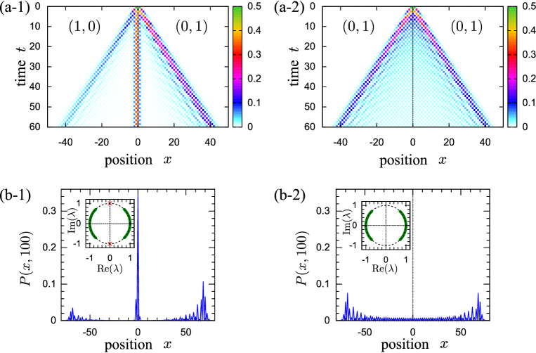
Figure 1: (Color online) Examples for bound states as signatures of a topological phase boundary in single step Hadamard walks. Top: Contour maps of the probability distribution $P(x,t)$ in $x-t$ plane for the quantum walks of (a-1) $U_{A}({\bm{\theta}}_{\alpha})$, Eq. (33), and (a-2) $U_{A}({\bm{\theta}}_{\beta})$, Eq. (34). The topological numbers $(\nu_{-\pi/2},\nu_{+\pi/2})$ for the negative and positive $x$ regions are shown in the figures. The position dependence of the probability distribution $P(x,t)$ at $t=100$ is shown in (b-1) and (b-2) for the single-step Hadamard walk $U_{A}({\bm{\theta}}_{\alpha})$ and $U_{A}({\bm{\theta}}_{\beta})$, respectively. The insets in (b-1) and (b-2) show eigenvalues $\lambda=e^{-i\varepsilon}$ of the corresponding time-evolution operator $U_{A}({\bm{\theta}}_{\alpha,\beta})$ of the main figure. The eigenvalues corresponding to edge states are distinguished by red crosses from those of bulk states (green thick arcs).

We first consider the simple Hadamard quantum walk, as defined in Eq. (7). We take a translation invariant bulk, with $\theta(x)=\theta$, in a chiral timeframe, as defined by Eq. (20). The operator $F_{A}$ at quasimomentum $k$ reads

$$F_{A}(k) =e^{-i\chi/2}e^{-i\theta/2\cdot\sigma_{2}}\begin{pmatrix}1&0\\ 0&e^{i(k+\chi)}\end{pmatrix}.$$ (26)

The parameter $\chi=\pi/2$ shows up in two roles here. First, it works as a global phase, $k$-independent factor. This cannot change the winding number. The second role is as a displacement of $k$ by $\chi$. This again does not change the winding number which is calculated by integrating over the whole $k$ space. Thereby, we are free to set $\chi=0$, when we substitute Eq. (26) into Eqs. (24) and (25). We obtain

$$\nu_{-\pi/2} =\frac{1}{2\pi i}\int_{-\pi}^{\pi}dk\frac{d}{dk}\text{ln }\left(s_{\theta+}\,-e^{ik}s_{\theta-}\right);$$ (27a)

$$\nu_{+\pi/2} =\frac{1}{2\pi i}\int_{-\pi}^{\pi}dk\frac{d}{dk}\text{ln }\left(s_{\theta-}\,+e^{ik}s_{\theta+}\right),$$ (27b)

using the shorthand

$$s_{\theta\pm} =\cos\frac{\theta}{2}\pm\sin\frac{\theta}{2}=\sqrt{2}\sin\frac{\theta\pm\pi/2}{2}.$$ (28)

The invariant at quasienergy $\pm\pi/2$ is the winding number of a loop on the complex plane, centered at $s_{\theta\pm}$ with radius $s_{\theta\mp}$. In the case in which the radius is larger than the distance of the center from the origin, the loop encircles the origin, and we have a winding number of $+1$. In the opposite case, the winding number is 0. Therefore, to calculate the values of the winding numbers, we need to consider

$$s_{\theta+}^{2}-s_{\theta-}^{2} =2\sin\theta.$$ (29)

For the winding numbers, the above considerations give

$$(\nu_{-\pi/2},\nu_{+\pi/2})=\left\{\begin{array}[]{rl}(0,1)&\quad\text{if}\quad 0<\theta<\pi,\\ (1,0)&\quad\text{if}\quad-\pi<\theta<0.\end{array}\right.$$ (32)

The topological invariants are not defined when $\theta=0$ or $\theta=\pi$. In these cases, the time-evolution operator reads $U_{A}(\theta=\pi/2\pm\pi/2)=\pm ie^{-i(k+\pi/2)\sigma_{3}},$ with a quasienergy spectrum that has no gaps.

Numerical examples

We illustrate the above results on the topology of the simple Hadamard walk, by showing examples where edge states appear near a boundary between two bulks with different topological invariants. To this end, we define two sets of $\theta(x)$:

$${\bm{\theta}}_{\alpha} :\{\theta_{-}=-\pi/4,\ \theta_{+}=+\pi/4\},$$ (33)

$${\bm{\theta}}_{\beta} :\{\theta_{-}=+3\pi/4,\ \theta_{+}=+\pi/4\},$$ (34)

where

$$\theta_{-}:=\theta(x\leq-1),\quad\theta_{+}:=\theta(x\geq 0).$$

According to Eq. (32), we expect that topologically protected edge states at quasienergies $\varepsilon=\pm\pi/2$ appear near $x\approx 0$ for $U_{A}({\bm{\theta}}_{\alpha})$, because the two bulk regions have different topological numbers, while no edge state should appear for $U_{A}({\bm{\theta}}_{\beta})$ because of the same topological numbers in both regions.

We numerically simulate the time evolution $|\Psi(t)\rangle=U_{A}^{t}|\Psi(t=0)\rangle$ up to $t=100$ and calculate the probability distribution

$$P(x,t):=\sum_{s=+,-}|(\langle x|\otimes\langle s|)|\Psi(t)\rangle|^{2}.$$ (35)

The initial state is set to

$$|\Psi(t=0)\rangle:=(|+\rangle+i|-\rangle)/\sqrt{2}\otimes|0\rangle.$$ (36)

Figures 1 (a-1) and (a-2) show the contour maps of $P(x,t)$ in the $x-t$ plane up to the time step $t=60$ for $U_{A}({\bm{\theta}}_{\alpha})$, Eq. (33), and $U_{A}({\bm{\theta}}_{\beta})$, Eq. (34) respectively. On the one hand, Fig. 1 (a-1) clearly shows that the high probability amplitudes stably remain near the origin where the topological numbers change. On the other hand, Fig. 1 (a-2) exhibits low probability amplitudes near $x=0$ as expected.

The presence/absence of edge states is further highlighted in Figs. 1 (b-1) and (b-2) showing snapshots of the probability distribution $P(x,t)$ at $t=100$ for $U_{A}({\bm{\theta}}_{\alpha})$ and $U_{A}({\bm{\theta}}_{\beta})$, respectively. We also numerically compute the spectrum of the timestep operators of the single-step Hadamard walks $U_{A}({\bm{\theta}}_{\alpha})$ and $U_{B}({\bm{\theta}}_{\beta})$, and show the eigenvalues $\lambda_{\varepsilon}=e^{-i\varepsilon}$ in the insets. Here we consider the finite position space from $-L$ to $L-1$ with $L=100$ and impose the periodic boundary conditions to $-L$ and $L-1$. Thereby, we have two boundaries at $x=0$ and $-L$, where $\theta(x)$ is varied. If one of these boundaries hosts an edge state at quasienergy $\varepsilon$, so must the other boundary: this gives an extra double degeneracy of the edge states. Although this degeneracy is lifted, because wavefunctions of the edge states at the same quasienergy but opposite edges overlap due to their exponential tails, this is the correction that is exponentially small in the system size, in our case, below the numerical accuracy $\sim 10^{-16}$. Consistent with our theoretical prediction, the eigenvalues corresponding to edge states (red crosses) appear at $\varepsilon=\pm\pi/2$ for $U_{A}({\bm{\theta}}_{\alpha})$, while they are not there for $U_{A}({\bm{\theta}}_{\beta})$. This illustrates the validity of Eq. (32).

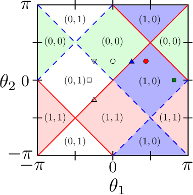
Figure 2: (Color online) The phase diagram of the split-step quantum walk $U_{B}(\theta_{1},\theta_{2})$ defined in Eq. (8). Gapped phases are indexed by topological numbers $(\nu_{0},\nu_{\pi})$, Eqs. (39). The red solid and blue dashed lines indicate closing of quasienergy gaps around $\varepsilon=0$ and $\pi$, respectively. The symbols in the phase diagram indicate the parameters of the numerical examples we consider, i.e., upper and lower triangles for ${\bm{\theta}}_{\gamma}$, ${\bm{\theta}}_{\delta}$ in Eqs. (41) and (40), circles for ${\bm{\theta}}_{e1}$ in Eq. (42), and rectangles for ${\bm{\theta}}_{e2}$ in Eq. (43).

IV.2 Split-step Hadamard walk

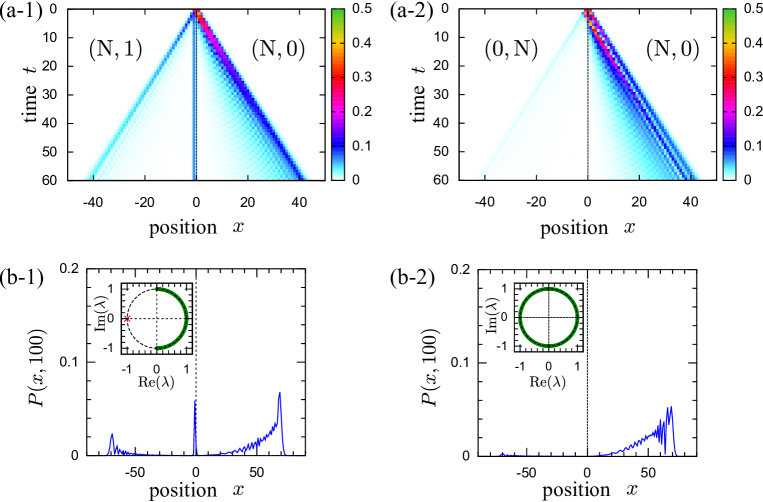
Figure 3: (Color online) Examples of bound states as signatures of a topological phase transition in split-step Hadamard walks. Top: Contour maps of the probability distribution $P(x,t)$ in the $x-t$ plane for the quantum walk (a-1) $U_{B}({\bm{\theta}}_{\gamma})$, Eq. (40) and (a-2) $U_{B}({\bm{\theta}}_{\delta})$, Eq. (41). The topological numbers $(\nu_{0},\nu_{\pi})$ for the negative and positive $x$ regions are shown in the figures. A letter “N” means that the topological number for the corresponding quasienergy cannot be defined because of the gap closing. (b) The position dependence of the probability distribution $P(x,t)$ at $t=100$. The eigenvalues of the timestep operators are shown in the insets as in Figs. 1 (b-1) and (b2).

We next consider the split-step Hadamard quantum walk, as defined in Eq. (8), with two coin operators $C_{\text{H}}[\theta_{1,2}(x)]$ applied during one timestep. We emphasize that this quantum walk has been realized in an optical experimentKitagawa et al. (2012). We take a translation invariant bulk, with $\theta_{j}(x)=\theta_{j}$, for both $j=1,2$, in a chiral timeframe, as defined by Eq. (21). The operator $F_{B}$ reads

$$F_{B} =e^{-i\chi}e^{-i\theta_{1}/2\cdot\sigma_{2}}\begin{pmatrix}1&0\\ 0&e^{i(k+2\chi)}\end{pmatrix}e^{-i\theta_{2}/2\cdot\sigma_{2}}.$$ (37)

Again, the parameter $\chi$ does not affect the winding numbers, then we can set $\chi=0$.

The calculation of the topological invariants follows the same lines as for the simple Hadamard walk. We substitute Eq. (37) into Eqs. (24) and (25). We obtain

$$\nu_{\pi} =\frac{1}{2\pi i}\int_{-\pi}^{\pi}dk\frac{d}{dk}\text{ln }\left(s_{\theta_{1}+}s_{\theta_{2}+}\,-e^{ik}s_{\theta_{1}-}s_{\theta_{2}-}\right);$$ (38a)

$$\nu_{0} =\frac{1}{2\pi i}\int_{-\pi}^{\pi}dk\frac{d}{dk}\text{ln }\left(\,s_{\theta_{1}-}s_{\theta_{2}+}\,+e^{ik}s_{\theta_{1}+}s_{\theta_{2}-}\right),$$ (38b)

using the shorthands defined in Eq. (28), and bearing in mind that the quasienergies are displaced by $\pi$ instead of $\pi/2$ as for the simple Hadamard walk.

Using the same logic as for the simple Hadamard walk for the winding numbers gives us

$$\nu_{\pi} =\left(\text{sign}[-\sin\theta_{1}-\sin\theta_{2}]+1\right)/2;$$ (39a)

$$\nu_{0} =\left(\text{sign}[\sin\theta_{1}-\sin\theta_{2}]+1\right)/2.$$ (39b)

The phase diagram in Fig. 2 of the topological numbers $\nu_{0}$ and $\nu_{\pi}$ at quasienergies $\varepsilon=0,\pi$, respectively, of $U_{B}(\theta_{1},\theta_{2})$.

Numerical examples

We illustrate the topological properties of the split-step Hadamard walk using two parameter sets,

$${\bm{\theta}}_{\gamma} :\{\theta_{1-}=\theta_{2-}=-\pi/4;\ \theta_{1+}=\theta_{2+}=+\pi/4\};$$ (40)

$${\bm{\theta}}_{\delta} :\{\theta_{1-}=-\theta_{2-}=-\pi/4;\ \theta_{1+}=\theta_{2+}=+\pi/4\},$$ (41)

where

$$\theta_{1(2)-}:=\theta_{1(2)}(x\leq-1),\quad\theta_{1(2)+}:=\theta_{1(2)}(x\geq 0).$$

Because only $\theta=\pm\pi/4$ is employed, the quantum walk $U_{B}({\bm{\theta}}_{\gamma,\delta})$ would be called the split-step Hadamard walk. As indicated by the triangles in Fig. 2, the parameters of the sets ${\bm{\theta}}_{\gamma,\delta}$ are located on the red solid and blue dashed lines indicating the quasienergy gap closing around $\varepsilon=0$ and $\pi$, respectively. In case of ${\bm{\theta}}_{\gamma}$, the quasienergy gap around $\varepsilon=0$ vanishes, while the other gap around $\varepsilon=\pi$ is still open. Since the topological numbers $\nu_{\pi}$ differ in the positive and negative $x$ regions for $U_{B}({\bm{\theta}}_{\gamma})$, the edge states should exist. However, in case of ${\bm{\theta}}_{\delta}$, parameters of the negative (positive) $x$ region locates on the blue dashed (red solid) line. This results in no more energy gaps in the whole system. Then, we predict no edge states for $U_{B}({\bm{\theta}}_{\delta})$.

We confirm these predictions from the phase diagram by numerical simulations as shown in Fig. 3. In case of $U_{B}({\bm{\theta}}_{\gamma})$, we confirm the edge state at the quasienergy $\varepsilon=\pi$ as well as the gap closing around $\varepsilon=0$. We also numerically confirm that no energy gaps emerge for $U_{B}({\bm{\theta}}_{\delta})$, and then no edge states.

V Interpretations of hidden topological invariants in experiment

Finally, we resolve the hidden topological invariant found in the photonic quantum walk experiment in Ref. Kitagawa et al., 2012 where the time-evolution operator is the one given in Eq. (8). We consider two parameter sets which are also investigated in the experimentKitagawa et al. (2012):

$${\bm{\theta}}_{e1}:\{ \theta_{1-}=0,\ \theta_{2-}=+\pi/4;$$

$$\quad\theta_{1+}=+7\pi/16,\ \theta_{2+}=+\pi/4\},$$ (42)

$${\bm{\theta}}_{e2}:\{ \theta_{1-}=-5\pi/16,\ \theta_{2-}=0;$$

$$\quad\theta_{1+}=+13\pi/16,\ \theta_{2+}=0\},$$ (43)

In Ref. Kitagawa et al., 2012, it is reported that the parameter spaces with the topological numbers $(1,0)$ and $(0,1)$ in Fig. 2 have the topological number $0$ and the regions with the topological number $(0,0)$ and $(1,1)$ in Fig. 2 have the topological number $1$. Thereby, in the case of ${\bm{\theta}}_{e1}$, the topological numbers of the positive and negative $x$ regions differ by $1$, and then edge states are expected. In the case of ${\bm{\theta}}_{e2}$, the topological numbers in both regions are zero, and then edge states are not expected. However, edge states are observed in both cases in the experiment.

In Fig. 4 (a) and (b), we show the probability distribution $P(x,t)$ at $t=100$ of the walks $U_{B}({\bm{\theta}}_{e1})$ and $U_{B}({\bm{\theta}}_{e2})$, respectively, starting from the initial state

$$|\psi(t=0)\rangle:=|+\rangle\otimes|0\rangle,$$

which also coincides with the experimental. The corresponding eigenvalues of $U_{B}({\bm{\theta}}_{e1})$ and $U_{B}({\bm{\theta}}_{e2})$ are shown in the insets. We confirm that the split-step walks $U_{B}({\bm{\theta}}_{e1})$ and $U_{B}({\bm{\theta}}_{e2})$ exhibit edge states at $\varepsilon=0$ and $\varepsilon=0,\pi$, respectively.

Now we look at the phase diagram in Fig. 2. The phase diagram predicts that the quantum walk $U_{B}({\bm{\theta}}_{e1})$ should have an edge state at $\varepsilon=0$ because the regions for $x\leq-1$ and $x\geq 0$ have the topological numbers $(\nu_{0},\nu_{\pi})=(0,0)$ and $(1,0)$, respectively. Furthermore, in the case of $U_{B}({\bm{\theta}}_{e2})$, the edge states should appear at quasienergies $\varepsilon=0,\pi$ because the regions for $x\leq-1$ and $x\geq 0$ have the topological numbers $(0,1)$ and $(1,0)$, respectively. These theoretical results are completely consistent with the numerical results in Fig. 4 and observations in the experimentKitagawa et al. (2012). Thereby, we have succeeded in explaining the hidden topological invariant found in the experiment by the phase diagram Fig. 2 which is derived by establishing the relation between the rotation and Hadamard matrices.

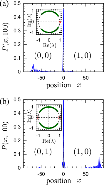
Figure 4: (Color online) The position dependence of the probability distribution $P(x,t)$ at $t=100$ is shown in (a) and (b) for the split-step walks $U_{B}({\bm{\theta}}_{e1})$ and $U_{B}({\bm{\theta}}_{e2})$, respectively. The topological numbers $(\nu_{0},\nu_{\pi})$ for the negative and positive $x$ regions are shown in the figures. The meaning of insets is the same as those in Figs. 1 (b-1) and (b2).

VI Discussions and conclusion

Comparing Fig. 1 (a-1) and (a-2) with Fig. 3 (a), we notice that the the contour maps of the probability distribution $P(x,t)$ in the former ones are sparser and checkerboard like. The origin of this is a sublattice symmetry of the time-evolution operator defined as

$${\Gamma_{S}}U{\Gamma_{S}}=-U,$$ (44)

where

$${\Gamma_{S}}:=(\sum_{x\in\text{even}}|x\rangle\langle x|-\sum_{x\in\text{odd}}|x\rangle\langle x|)\otimes\sigma_{0}.$$

The single step walk $U_{A}$ retains sublattice symmetry, while the split-step walk $U_{B}$ generally does not. This symmetry constrains the walker at every timestep to hop from the even sublattice ($x$ even) to the odd sublattice ($x$ odd), leading to the checkerboard pattern of $P(x,t)$.

If a quantum walk has sublattice symmetry, as defined by Eq. (44), every eigenstate at quasienergy $\varepsilon$ must have a sublattice partner at quasienergy $\varepsilon+\pi$Obuse and Kawakami (2011); Shikano and Katsura (2010). This explains why the single step Hadamard walk has edge states at $\varepsilon=\pm\pi/2$ appearing simultaneously. We note that, due to the specific value of $\theta_{2}=0$ in the parameter set ${\bm{\theta}}_{e2}$, the split-step walk $U_{B}({\bm{\theta}}_{e2})$ has sublattice symmetry. Therefore, the edge states appearing at $\varepsilon=0,\pi$ in the inset of Fig. 4 (b) are sublattice symmetric partners of each other.

The results of this manuscript can be applied straightforwardly to quantum walks where the generalized Hadamard coin is replaced by operators $e^{-i\theta\sigma_{2}}\sigma_{j}$, with $j=1,2$, instead of $j=3$. In the case of $j=2$, we again obtain a chiral symmetric walk: in analogy with Eq. (17), we have

$$e^{-i\theta\sigma_{2}}\sigma_{2} = e^{-i\phi}e^{-i(\theta+\eta)\sigma_{2}},$$ (45)

where $\eta=-\phi=\pi/2$. Thereby, $\sigma_{2}$ shifts the angle of the rotation matrix and the quasienergy by $\pi/2$, but does not affect chiral symmetry. The other case, $j=1$, is easily understood because $\sigma_{1}=-i\sigma_{2}\sigma_{3}$. Using Eqs. (17) and (45), we obtain

$$e^{-i\theta\sigma_{2}}\sigma_{1}=e^{-i\phi}e^{-i(\theta+\eta)\sigma_{2}}\cdot e^{-i\chi\sigma_{3}},$$ (46)

where $\eta=\chi=-\phi=\pi/2$ are global and fixed parameters. Thereby, $\sigma_{1}$ also does not break chiral symmetry.

In Ref. Kitagawa et al., 2012, two topological invariants, $Q^{0}$ and $Q^{\pi}$ are defined that are associated with a boundary between two bulks. These invariants are nothing but the topologically protected number of 0 and $\pi$ quasienergy edge states localized at the boundary. The topological invariants $\nu_{0}$ and $\nu_{\pi}$ we define in this paper are associated with the bulks. By the arguments detailed in Ref. Asbóth and Obuse, 2013, the change in $\nu_{0}$ ($\nu_{\pi}$) as we cross from the left bulk to the right predicts the value of $Q^{0}$ ($Q^{\pi}$): this is the bulk–boundary correspondence for one-dimensional Hadamard quantum walks.

The formulas for the topological invariants in this paper assumed translation invariance in the bulk, so that the quasi-momentum $k$ is a good quantum number. For disordered quantum walks, e.g., where $\theta(x)$ is a random function of position, there are alternative formulations of the topological invariants, based on the scattering matricesTarasinski et al. (2014); Rakovszky and Asboth (2015). These can be applied to disordered Hadamard walks using the mapping we presented in this paper.

In summary, we have studied the topological phases of the one-dimensional Hadamard quantum walk. We have generalized the definition of chiral symmetry, and provided a sufficient requirement for quantum walks to obey this symmetry, in Eq. (15). Employing the generalized definition, one-dimensional Hadamard quantum walks have chiral symmetry, and the corresponding topological invariants, which characterize the topological phases, can be calculated. We have used this result to reveal the topological invariants behind a recent photonic quantum walk experimentKitagawa et al. (2012). Our results add to the growing body of knowledge on the topological phases of quantum walks and Floquet topological insulators.

VII Acknowledgments

We thank T. Endo and N. Konno for helpful discussions. H. O. was supported by Grant-in-Aid (No. 25800213 and N. 25390113) from the Japan Society for Promotion of Science, J. K. A. by the Hungarian Academy of Sciences (Lendület Program, LP2011-016), by the Hungarian Scientific Research Fund (OTKA) under Contract No. NN109651, and by the Janos Bolyai scholarship. The work of N. K. was supported by Grant-in-Aid (No. 25400366 and No. 15H05855) from the Japan Society for Promotion of Science.

Appendix A Alternative calculation of topological numbers

In Sec. IV, we calculate the topological numbers of the quantum walks based on the method developed in Ref. Asbóth et al., 2014. Here, for completeness, we present the calculation following the method of Ref. Asbóth and Obuse, 2013. The two methods are equivalent, we present this derivation for pedagogical reasons.

A.1 Single-step Hadamard walk

First, we focus on the single-step Hadamard walk. From Eq. (20a), the chiral symmetric form of the single-step Hadamard walk is written as

$$U_{A} = e^{-i\phi}\cdot F_{A}\cdot\Gamma F_{A}^{-1}\Gamma,$$ (47)

$$F_{A} = e^{-i\theta(x)/2\cdot\sigma_{2}}\cdot e^{-i\chi/2\cdot\sigma_{3}}S_{-},$$

$$\Gamma F_{A}^{-1}\Gamma = S_{+}\cdot e^{-i\chi/2\cdot\sigma_{3}}\cdot e^{-i\theta(x)/2\cdot\sigma_{2}},$$

where $\chi=-\phi=\pi/2$. As explained in Ref. Asbóth and Obuse, 2013, if a time-evolution operator of the quantum walk $U$ has chiral symmetry, another chiral symmetric time-evolution operator $U^{\prime}$ can be identified only at the different “timeframe”. The one for $U_{A}$, thus $U_{A}^{\prime}$, is given by

$$U_{A}^{\prime} = e^{-i\phi}\cdot\Gamma F_{A}^{-1}\Gamma\cdot F_{A}.$$ (48)

Since the phase $\phi$ only shifts the quasienergy, we proceed in our calculations by setting $\phi=0$ on the above equations during the calculation and shift the quasienergy by $\pi/2$ at the end. In the momentum representation (by assuming the constant $\theta$), we have

$$U_{A}(k) = e^{-i\theta/2\cdot\sigma_{2}}\begin{pmatrix}e^{-i(k+\chi)}&0\\ 0&e^{ik(k+\chi)}\end{pmatrix}e^{-i\theta/2\cdot\sigma_{2}}$$

$$= \cos(k+\chi)c_{\theta}\sigma_{0}-ic_{k}s_{\theta}\sigma_{2}-i\sin(k+\chi)\sigma_{3},$$

and

$$U_{A}^{\prime}(k) = \begin{pmatrix}e^{-i(k+\chi)}&0\\ 0&1\end{pmatrix}e^{-i\theta\cdot\sigma_{2}}\begin{pmatrix}1&0\\ 0&e^{i(k+\chi)}\end{pmatrix}$$

$$= \cos(k+\chi)c_{\theta}\sigma_{0}-is_{\theta}\sigma_{2}-i\sin(k+\chi)c_{\theta}\sigma_{3}.$$

Here, we use the shorthands

$$c_{\theta}\equiv\cos(\theta),\quad s_{\theta}\equiv\sin(\theta).$$

The factor $\chi$ only shifts the momentum $k$, which does not change the topological number. Then, we set $\chi=0$ in the following.

Applying a unitary transform so that the time evolution operators have chiral symmetry in the basis that the chiral symmetry operator is diagonal, i.e., $\Gamma=\sigma_{3}$, we have

$$\tilde{U}_{A}(k) = e^{i\pi/4\cdot\sigma_{2}}U_{A}(k)e^{-i\pi/4\cdot\sigma_{2}}$$

$$= c_{k}c_{\theta}\sigma_{0}+is_{k}\sigma_{1}-ic_{k}s_{\theta}\sigma_{2},$$

and

$$\tilde{U}_{A}^{\prime}(k) = e^{i\pi/4\cdot\sigma_{2}}U_{A}^{\prime}(k)e^{-i\pi/4\cdot\sigma_{2}}$$

$$= c_{k}c_{\theta}\sigma_{0}+is_{k}c_{\theta}\sigma_{1}-is_{\theta}\sigma_{2}.$$

Since the coefficients of the $\sigma_{0}$ term of $\tilde{U}_{A}(k)$ and $\tilde{U}_{A}^{\prime}(k)$ are the same, both operators have a common eigenvalue

$$\lambda_{A,\pm}=e^{\pm i\omega_{A}},\quad\sin(\omega_{A})=\sqrt{1-(c_{k}c_{\theta})^{2}}\geq 0.$$

The corresponding eigenvectors $|{\psi_{\pm}}\rangle$ and $|{\psi_{\pm}^{\prime}}\rangle$ of $\tilde{U}_{A}(k)$ and $\tilde{U}_{A}^{\prime}(k)$, respectively, also have the similar structures

$$|{\psi_{A,\pm}}\rangle=\frac{1}{\sqrt{2}}\begin{pmatrix}\mp ie^{i\varphi_{A}(k)}\\ 1\end{pmatrix},|{\psi^{\prime}_{A,\pm}}\rangle=\frac{1}{\sqrt{2}}\begin{pmatrix}\mp ie^{i\varphi_{A}^{\prime}(k)}\\ 1\end{pmatrix},$$ (49)

but with different phase factors

$$e^{i\varphi_{A}(k)} =(-c_{k}s_{\theta}+is_{k})/\sin(\omega_{A}),$$ (50a)

$$e^{i\varphi_{A}^{\prime}(k)} =(-s_{\theta}+is_{k}c_{\theta})/\sin(\omega_{A}).$$ (50b)

The winding number is defined through the Berry phase,

$$\nu\equiv\frac{1}{i\pi}\int dk\langle{\psi}|d/dk|{\psi}\rangle.$$ (51)

Substituting eigenvectors in Eq. (49), the winding numbers $\nu$ and $\nu^{\prime}$ of $U_{A}$ and $U_{A}^{\prime}$, respectively, become

$$\nu=\frac{1}{2\pi}\oint d\varphi_{A}(k),\quad\nu^{\prime}=\frac{1}{2\pi}\oint d\varphi_{A}^{\prime}(k).$$

Thereby, the winding numbers are determined from the trace of $\varphi_{A}(k)$ and $\varphi_{A}^{\prime}(k)$ as $k$ is changed from $0$ to $2\pi$. Considering Eq. (50), this gives the following results,

$$\nu=\left\{\begin{array}[]{rr}-1&(0<\theta<\pi)\\ 1&(-\pi<\theta<0)\end{array}\right.,$$

and

$$\nu^{\prime}=0.$$

Finally by using a formula derived in Ref. Asbóth and Obuse, 2013 in order to calculate the topological numbers for quasienergies $\varepsilon=\phi$ and $\pi+\phi$

$$\nu_{\phi}=\frac{\nu^{\prime}+\nu}{2},\quad\nu_{\pi+\phi}=\frac{\nu^{\prime}-\nu}{2},$$ (53)

we obtain

$$(\nu_{-\pi/2},\nu_{+\pi/2})=\left\{\begin{array}[]{rl}(-1/2,+1/2)&\quad\text{for }0<\theta<\pi\\ (+1/2,-1/2)&\quad\text{for }-\pi<\theta<0.\end{array}\right.$$ (54)

Since the global shift of topological numbers does not alter the argument of the bulk-edge correspondence, we confirm the consistent result with Eq. (32) in Sec. IV by shifting numbers in the right side of Eq. (54) by $1/2$.

A.2 Split-step Hadamard walk

In the case of the split-step Hadamard walk, we have the following two chiral symmetric time-evolution operators

$$U_{B} =e^{-i2\phi}\cdot F_{B}\cdot\Gamma F_{B}^{-1}\Gamma,$$ (55)

$$U_{B}^{\prime} =e^{-i2\phi}\cdot\Gamma F_{B}^{-1}\Gamma\cdot F_{B},$$ (56)

where

$$F_{B} =e^{-i\theta_{1}(x)/2\cdot\sigma_{2}}S_{-}\cdot e^{-i\chi\sigma_{3}}\cdot e^{-i\theta_{2}(x)/2\cdot\sigma_{2}},$$

$$\Gamma F_{B}^{-1}\Gamma =e^{-i\theta_{2}(x)/2\cdot\sigma_{2}}\cdot e^{-i\chi\sigma_{3}}S_{+}\cdot e^{-i\theta_{1}(x)/2\cdot\sigma_{2}},$$

with $\chi=-\phi=\pi/2$. Again we set $\phi=0$ of $U_{B}$ and $U_{B}^{\prime}$ and shift the quasienergy by $\pi$ at the end of the calculation. We derive the time evolution operators in the momentum space representation as

$$U_{B}(k) = [\cos(k+2\chi)c_{\theta_{2}}c_{\theta_{1}}-s_{\theta_{2}}s_{\theta_{1}}]\sigma_{0}$$ (57)

$$- i[\cos(k+2\chi)c_{\theta_{2}}s_{\theta_{1}}+s_{\theta_{2}}c_{\theta_{1}}]\sigma_{2}$$

$$- i\sin(k+2\chi)c_{\theta_{2}}\sigma_{3},$$

and

$$U_{B}^{\prime}(k) = [\cos(k+2\chi)c_{\theta_{2}}c_{\theta_{1}}-s_{\theta_{2}}s_{\theta_{1}}]\sigma_{0}$$

$$- i[\cos(k+2\chi)c_{\theta_{1}}s_{\theta_{2}}+s_{\theta_{1}}c_{\theta_{2}}]\sigma_{2}$$

$$- i\sin(k+2\chi)c_{\theta_{1}}\sigma_{3}.$$

Comparing the above two equations, we notice that $U_{B}(k)$ and $U_{B}^{\prime}(k)$ are identical only by switching $\theta_{1}$ and $\theta_{2}$. This means that results for $U_{B}(k)$ are immediately applied to those for $U_{B}^{\prime}(k)$ by switching $\theta_{1}$ and $\theta_{2}$. Thereby, we present calculations only for $U_{B}(k)$ hereafter.

Similarly to the single-step Hadamard walk case, we can set $\chi=0$ in Eq. (57) and apply the unitary transformation, we have

$$\tilde{U}_{B}(k) = e^{i\pi/4\cdot\sigma_{2}}U_{B}(k)e^{-i\pi/4\cdot\sigma_{2}}$$

$$= [\cos(k)c_{\theta_{2}}c_{\theta_{1}}-s_{\theta_{2}}s_{\theta_{1}}]\sigma_{0}$$

$$+ i\sin(k)c_{\theta_{2}}\sigma_{1}$$

$$- i[\cos(k)c_{\theta_{2}}s_{\theta_{1}}+s_{\theta_{2}}c_{\theta_{1}}]\sigma_{2}.$$

The eigenvalue of $\tilde{U}_{B}(k)$ is

$$\lambda_{B,\pm} = e^{\pm i\omega_{B}},$$

$$\sin(\omega_{B}) = \sqrt{1-[\cos(k)c_{\theta_{2}}c_{\theta_{1}}-s_{\theta_{2}}s_{\theta_{1}}]^{2}}\geq 0,$$

and the corresponding eigenvector is

$$|{\psi_{B,\pm}}\rangle = \frac{1}{\sqrt{2}}\begin{pmatrix}\mp ie^{i\varphi_{B}(k)}\\ 1\end{pmatrix},$$ (58)

$$e^{i\varphi_{B}(k)} = \frac{-[\cos(k)c_{\theta_{2}}s_{\theta_{1}}+s_{\theta_{2}}c_{\theta_{1}}]+i\sin(k)c_{\theta_{2}}}{\sin(\omega_{B})}.$$

Substituting Eq. (58) into Eq. (51), the winding number $\nu$ of $U_{B}$ is summarized as follows: when

$$\sin^{2}(\theta_{1})-\sin^{2}(\theta_{2})>0,$$ (59)

$$\nu=\left\{\begin{array}[]{rr}-1&(0<\theta_{1}<\pi)\\ 1&(-\pi<\theta_{1}<0)\end{array}\right.,$$ (62)

otherwise

$$\nu=0.$$ (63)

As we mentioned, the winding number $\nu^{\prime}$ of $U_{B}^{\prime}(k)$ is given by switching $\theta_{1}$ and $\theta_{2}$ in the above results for $\nu$.

Finally, we obtain the consistent phase diagram with that of Fig. 2 in Sec. IV, by substituting $\nu$ and $\nu^{\prime}$ of $U_{B}$ and $U_{B}^{\prime}$, respectively, into Eq. (53), taking account of the quasienergy shift by $\pi$, and $1/2$ shift of the topological numbers.

References

- Hasan and Kane (2010) M. Z. Hasan and C. L. Kane, Rev. Mod. Phys. 82, 3045 (2010).
- Qi and Zhang (2011) X.-L. Qi and S.-C. Zhang, Rev. Mod. Phys. 83, 1057 (2011).
- Kitagawa et al. (2010a) T. Kitagawa, E. Berg, M. Rudner, and E. Demler, Phys. Rev. B 82, 235114 (2010a).
- H. et al. (2011) L. N. H., G. Refael, and V. Galitski, Nature Physics 7, 490–495 (2011).
- Cayssol et al. (2013) J. Cayssol, B. Dóra, F. Simon, and R. Moessner, Phys. Status Solidi RRL 7, 101 (2013).
- Rudner et al. (2013) M. S. Rudner, N. H. Lindner, E. Berg, and M. Levin, Phys. Rev. X 3, 031005 (2013).
- Schnyder et al. (2008) A. P. Schnyder, S. Ryu, A. Furusaki, and A. W. W. Ludwig, Phys. Rev. B 78, 195125 (2008).
- Kitaev (2009) A. Kitaev, in AIP Conf. Proc, 1134 (2009) p. 22.
- Ryu et al. (2010) S. Ryu, A. P. Schnyder, A. Furusaki, and A. W. W. Ludwig, New Journal of Physics 12, 065010 (2010).
- Rechtsman et al. (2013) M. C. Rechtsman, J. M. Zeuner, Y. Plotnik, Y. Lumer, D. Podolsky, F. Dreisow, S. Nolte, M. Segev, and A. Szameit, Nature 496, 196 (2013).
- Wang et al. (2013) Y. Wang, H. Steinberg, P. Jarillo-Herrero, and N. Gedik, Science 342, 453 (2013).
- Jotzu et al. (2014) G. Jotzu, M. Messer, R. Desbuquois, M. Lebrat, T. Uehlinger, D. Greif, and T. Esslinger, Nature 515, 237 (2014).
- Aidelsburger et al. (2013) M. Aidelsburger, M. Atala, M. Lohse, J. T. Barreiro, B. Paredes, and I. Bloch, Physical review letters 111, 185301 (2013).
- Kempe (2003) J. Kempe, Contemporary Physics 44, 307 (2003).
- Ambainis (2003) A. Ambainis, Int. J. Quantum Inform. 01, 507 (2003).
- Karski et al. (2009) M. Karski, L. Förster, J.-M. Choi, A. Steffen, W. Alt, D. Meschede, and A. Widera, Science 325, 174 (2009), http://www.sciencemag.org/content/325/5937/174.full.pdf .
- Schmitz et al. (2009) H. Schmitz, R. Matjeschk, C. Schneider, J. Glueckert, M. Enderlein, T. Huber, and T. Schaetz, Phys. Rev. Lett. 103, 090504 (2009).
- Zähringer et al. (2010) F. Zähringer, G. Kirchmair, R. Gerritsma, E. Solano, R. Blatt, and C. F. Roos, Phys. Rev. Lett. 104, 100503 (2010).
- Schreiber et al. (2010) A. Schreiber, K. N. Cassemiro, V. Potoček, A. Gábris, P. J. Mosley, E. Andersson, I. Jex, and C. Silberhorn, Phys. Rev. Lett. 104, 050502 (2010).
- Schreiber et al. (2012) A. Schreiber, A. Gábris, P. P. Rohde, K. Laiho, M. Štefaňák, V. Potoček, C. Hamilton, I. Jex, and C. Silberhorn, Science 336, 55 (2012), http://www.sciencemag.org/content/336/6077/55.full.pdf .
- Broome et al. (2010) M. A. Broome, A. Fedrizzi, B. P. Lanyon, I. Kassal, A. Aspuru-Guzik, and A. G. White, Phys. Rev. Lett. 104, 153602 (2010).
- Crespi et al. (2013) A. Crespi, R. Osellame, R. Ramponi, V. Giovannetti, R. Fazio, L. Sansoni, F. D. Nicola, F. Sciarrino, and P. Mataloni, Nat. Phot. 7, 322– (2013).
- Kitagawa et al. (2010b) T. Kitagawa, M. S. Rudner, E. Berg, and E. Demler, Phys. Rev. A 82, 033429 (2010b).
- Kitagawa (2012) T. Kitagawa, Quantum Information Processing 11, 1107 (2012).
- Obuse and Kawakami (2011) H. Obuse and N. Kawakami, Phys. Rev. B 84, 195139 (2011).
- Asbóth (2012) J. K. Asbóth, Phys. Rev. B 86, 195414 (2012).
- Asbóth and Obuse (2013) J. K. Asbóth and H. Obuse, Phys. Rev. B 88, 121406 (2013).
- Tarasinski et al. (2014) B. Tarasinski, J. Asbóth, and J. P. Dahlhaus, Phys. Rev. A 89, 042327 (2014).
- Edge and Asboth (2015) J. M. Edge and J. K. Asboth, Phys. Rev. B 91, 104202 (2015).
- Asboth and Edge (2015) J. K. Asboth and J. M. Edge, Phys. Rev. A 91, 022324 (2015).
- Chandrashekar et al. (2015) C. M. Chandrashekar, H. Obuse, and T. Busch, arXiv:1502.00436 (2015).
- Kitagawa et al. (2012) T. Kitagawa, M. A. Broome, A. Fedrizzi, M. S. Rudner, E. Berg, I. Kassal, A. Aspuru-Guzik, E. Demler, and A. G. White, Nature Communications 3, 882 (2012).
- Asbóth et al. (2014) J. Asbóth, B. Tarasinski, and P. Delplace, Physical Review B 90, 125143 (2014).
- Shikano and Katsura (2010) Y. Shikano and H. Katsura, Physical Review E 82, 031122 (2010).
- Rakovszky and Asboth (2015) T. Rakovszky and J. K. Asboth, arXiv preprint arXiv:1505.04513 (2015).